FTUAM-99/21

IASSNS-HEP-99/61

IFT-UAM/CSIC-99-25

hep-th/9907074

${\cal N}=1$ Type IIA brane configurations,
Chirality and T-duality
J. Park${}^{{\dagger}\,}$, R. Rabadán${}^{\S\,}$ and A. M. Uranga${}^{{\dagger}\,}$
^† School of Natural Sciences, Institute for Advanced Study,
Olden Lane, Princeton NJ 08540, USA.
^§ Departamento. de Física Teórica C-XI and Instituto de Física Teórica C-XVI,
Universidad Autónoma de Madrid, Cantoblanco, 28049 Madrid, Spain.
Abstract

We consider four-dimensional ${\cal N}=1$ field theories realized by type IIA brane configurations of NS-branes and D4-branes, in the presence of orientifold six-planes and D6-branes. These configurations are known to present interesting effects associated to the appearance of chiral symmetries and chiral matter in the four-dimensional field theory. We center on models with one compact direction (elliptic models) and show that, under T-duality, the configurations are mapped to a set of type IIB D3-branes probing ${\cal N}=1$ orientifolds of $\bf C^{2}/\bf Z_{N}$ singularities. We explicitly construct these orientifolds, and show the field theories on the D3-brane probes indeed reproduces the field theories constructed using the IIA brane configurations. This T-duality map allows to understand the type IIB realization of several exotic brane dynamics effects on the type IIA side: Flavour doubling, the splitting of D6-branes and O6-planes in crossing a NS-brane and the effect of a non-zero type IIA cosmological constant turn out to have surprisingly standard type IIB counterparts.

1 Introduction

One of the most interesting features of four-dimensional field theories that has been successfully reproduced in their realization in string theory is the appearance of chiral matter and chiral symmetries. The first realizations of ${\cal N}=1$ supersymmetric gauge field theories in terms of brane configurations, in the spirit of [1], involved a set of type IIA D4-branes (along the directions 01236), relatively rotated NS-fivebranes (along 012345 or 012389), and D6-branes (along 0123789) [2] (see review for further references). However, given their close relation with the ${\cal N}=2$ models in [4] via a rotation of NS-branes [5] which makes the adjoint matter massive, they have vector-like matter content. Also, the chiral symmetries present in the field theory for massless flavours are not manifest in the brane realization.

The second of these issues was further explored in [6], where it was noticed that the fundamental flavours arising from the D6-branes have generically quartic superpotential interactions, mediated by the massive adjoints, which only preserve the diagonal vector-like subgroup of the chiral symmetry. This superpotential can however be varied by rotating the D6-branes in the 45-89 plane, and vanishes for D6-branes oriented along 0123457 (D6^′-branes) . The chiral symmetries in the field theory were argued to be manifest in the brane configuration when the D6^′ branes are located on top of the NS-branes and split in half D6^′-branes, of semi-infinite extent in the direction 7. The independent gauge symmetries on these ‘upper ’ and ‘lower’ half D6^′-branes correspond to the independent chiral rotations of the matter multiplets, leading to the conclusion that one half D6^′-brane, ending on a NS-brane with D4-branes suspended on it, leads to one chiral fundamental multiplet in the four-dimensional field theory . Unfortunately, the inability of the NS-branes to carry away the RR charge of the half D6^′-branes requires the number of upper and lower half-branes to be identical, implying vector-like matter contents.

A further step was taken in [8], where it was pointed out that the presence of a non-zero type IIA cosmological constant (so that the configuration is actually embedded in massive type IIA theory) forces a mismatch between the number of upper and lower half D6^′-branes (equal to the value of the cosmological constant in appropriate units), which allows to obtain chiral matter localized at these intersections. In this setup quite exotic phase transitions were shown to occur, in which the number of chiral multiplets changes due to a change in the IIA cosmological constant. The latter is achieved by introducing D8-branes (along 012345689), which behave as domain walls across which the cosmological constant changes, and crossing them through the configuration. In these initial models, however, overall conservation of RR charge implied the complete matter content must be vector-like, even though fundamental and anti-fundamental chiral multiplets are generically localized at spatially different positions in the direction 6. From the field theory point of view the vector-like matter content is merely consequence of cancellation of gauge anomalies, since the configuration only allow to obtain fundamental and anti-fundamental representations.

The final ingredient to achieve chiral matter contents was the introduction of orientifold planes parallel to the D6^′-branes (O6^′-planes), since they allow the appearance of two-index tensor representations. Specifically, when an O6^′-plane sits on top of a NS-brane, its two halves have opposite RR charge [9]. Due to the different orientifold projection in the upper and lower halves in $x^{7}$, there appears chiral matter multiplets transforming in the $\raisebox{-0.5pt}{\hbox{\rule{0.4pt}{6.5pt}\hskip-0.4pt\rule{6.5pt}{0.4pt}\hskip-6.5pt\rule[6.5pt]{6.5pt}{0.4pt}}\rule[6.5pt]{0.4pt}{0.4pt}\hskip-0.4pt\rule{0.4pt}{6.5pt}}\hskip-0.4pt\raisebox{-0.5pt}{\hbox{\rule{0.4pt}{6.5pt}\hskip-0.4pt\rule{6.5pt}{0.4pt}\hskip-6.5pt\rule[6.5pt]{6.5pt}{0.4pt}}\rule[6.5pt]{0.4pt}{0.4pt}\hskip-0.4pt\rule{0.4pt}{6.5pt}}+\overline{\raisebox{-3.5pt}{\hbox{\rule{0.4pt}{6.5pt}\hskip-0.4pt\rule{6.5pt}{0.4pt}\hskip-6.5pt\rule[6.5pt]{6.5pt}{0.4pt}}\rule[6.5pt]{0.4pt}{0.4pt}\hskip-0.4pt\rule{0.4pt}{6.5pt}}\hskip-6.9pt\raisebox{3.0pt}{\hbox{\rule{0.4pt}{6.5pt}\hskip-0.4pt\rule{6.5pt}{0.4pt}\hskip-6.5pt\rule[6.5pt]{6.5pt}{0.4pt}}\rule[6.5pt]{0.4pt}{0.4pt}\hskip-0.4pt\rule{0.4pt}{6.5pt}}}$ representation [10, 11, 12]. Finally, overall conservation of RR charge (or anomaly cancellation in the field theory) implies the existence of additional half D6^′-branes producing eight anti-fundamental chiral flavours , localized either at the same position in the direction 6 (for zero IIA cosmological constant) or elsewhere (for non-zero cosmological constant). This type of dynamics of D6-branes and O6-planes has also appeared in the context of type IIA brane configurations realizing six-dimensional supersymmetric field theories [14, 15, 16].

Despite this success, which allows to realize a chiral gauge field theory in string theory, and to analyze its M-theory lift [17, 18], the type IIA approach is extremely rigid and has not allowed to construct further examples of chiral theories . Completely different setups, like type IIB brane box models [20], and their T-dual realization in terms of D3-brane probes at threefold singularities [22, 23, 24] (and orientifolds thereof [29]) have proved more efficient in producing generically chiral field theories.

Two conclusions can be drawn from this brief review. The first is the surprising amount, diversity and apparent ‘exotism’ of the non-trivial effects required in the type IIA setup to reproduce models with chiral symmetries and chiral matter content. The second is the apparent extreme isolation of the chiral gauge theory constructed in the IIA setup using the change of sign of the O6^′-plane. It seems to be rather unrelated to other configurations in string theory realizing four-dimensional chiral gauge theories.

In this paper we provide some insight into these issues. We consider type IIA configurations of NS-branes (along 012345), D4-branes (along 01236), and D6^′-branes and O6^′-planes (along 0123457), with the direction 6 compactified on a circle. These can be regarded as the ${\cal N}=2$ elliptic models of [4] in the presence of O6^′-planes which break the supersymmetry to ${\cal N}=1$. We study the resulting type IIB string theory configurations obtained upon T-dualizing along this compact direction. They correspond to ${\cal N}=1$ orientifolds of a system of D3-branes at a $\bf C^{2}/\bf Z_{N}$ singularity. We explicitly classify and construct these orientifolds, and show they indeed realize the field theories obtained from the type IIA configurations. The matching of both types of models allows to find the type IIB counterparts of the non-trivial brane dynamics effects present in the IIA models. The correct chiral matter content and pattern of chiral symmetries are reproduced by the completely standard rules of IIB orientifold construction. We list here the main results:

• We find that half D6^′-branes map to whole D7-branes. Concretely, upper and lower half D6^′-branes map to D7-branes along either of the two complex planes in $\bf C^{2}/\bf Z_{N}$. The chiral symmetries in the field theory (gauge symmetries on the half D6^′-branes) appear as gauge symmetries on the D7-branes .

• The phenomenon of flavour doubling is reproduced by the fact that one D7-brane produces two fundamental chiral flavours arising from the 3-7 and 7-3 sectors .

• The matter content $\raisebox{-0.5pt}{\hbox{\rule{0.4pt}{6.5pt}\hskip-0.4pt\rule{6.5pt}{0.4pt}\hskip-6.5pt\rule[6.5pt]{6.5pt}{0.4pt}}\rule[6.5pt]{0.4pt}{0.4pt}\hskip-0.4pt\rule{0.4pt}{6.5pt}}\hskip-0.4pt\raisebox{-0.5pt}{\hbox{\rule{0.4pt}{6.5pt}\hskip-0.4pt\rule{6.5pt}{0.4pt}\hskip-6.5pt\rule[6.5pt]{6.5pt}{0.4pt}}\rule[6.5pt]{0.4pt}{0.4pt}\hskip-0.4pt\rule{0.4pt}{6.5pt}}+\overline{\raisebox{-3.5pt}{\hbox{\rule{0.4pt}{6.5pt}\hskip-0.4pt\rule{6.5pt}{0.4pt}\hskip-6.5pt\rule[6.5pt]{6.5pt}{0.4pt}}\rule[6.5pt]{0.4pt}{0.4pt}\hskip-0.4pt\rule{0.4pt}{6.5pt}}\hskip-6.9pt\raisebox{3.0pt}{\hbox{\rule{0.4pt}{6.5pt}\hskip-0.4pt\rule{6.5pt}{0.4pt}\hskip-6.5pt\rule[6.5pt]{6.5pt}{0.4pt}}\rule[6.5pt]{0.4pt}{0.4pt}\hskip-0.4pt\rule{0.4pt}{6.5pt}}}+8\overline{\raisebox{-0.5pt}{\hbox{\rule{0.4pt}{6.5pt}\hskip-0.4pt\rule{6.5pt}{0.4pt}\hskip-6.5pt\rule[6.5pt]{6.5pt}{0.4pt}}\rule[6.5pt]{0.4pt}{0.4pt}\hskip-0.4pt\rule{0.4pt}{6.5pt}}}$ in the chiral theories is correctly reproduced in the IIB setup. The IIB orientifold also encodes the structures of O6^′-planes in the upper and lower halves in $x^{7}$, in terms of the orientifold action on the two complex planes in $\bf C^{2}/\bf Z_{N}$. The type IIB orientifold configurations are, in contrast with the type IIA models, quite smooth and do not present abrupt changes in the orientifold type.

• Cancellation of anomalies in the field theory (conservation of RR charge in the IIA configuration) corresponds to cancellation of tadpoles for twisted RR fields in the IIB model.

• We also find the type IIB T-dual of the type IIA cosmological constant. The transitions changing the number of field theory flavours are interpreted as a brane creation process in the type IIB side.

Thus, several rather ‘exotic’ effects in the type IIA brane configurations are reproduced by completely standard rules in the context of type IIB orientifold construction. This also sheds some light on the issue of the isolation of these chiral field theories. In the type IIB realization as D3-branes probing orientifold singularities, these models do not differ in any essential way from the constructions yielding generically chiral field theories (for instance D3-branes probes at $\bf C^{3}/\Gamma$ threefold orbifold singularities and orientifolds thereof). This point becomes even clearer by noticing that both types of models are actually continuously connected [31]: Some configurations of D3-branes at orientifolds of $\bf C^{3}/\Gamma$ reduce, after suitable partial resolutions of the singularity, to the orientifolds of $\bf C^{2}/\bf Z_{N}$ appearing in this paper; from the field theory point of view this is realized a suitable baryonic Higgs breaking that relates both field theories. Therefore, our realization of these models in the singularity picture points towards a more unified description of all string theory configurations producing four-dimensional chiral field theories.

A last advantage of having a realization of these gauge theories in terms of D3-brane probes at singularities is that it is well-suited for the study of the field theory in the large $N$ limit through the AdS/CFT correspondence [32].

The paper is organized as follows. In Section 2 we construct type IIA configurations of NS-branes, D4-branes and D6^′-branes, with one compact direction but without orientifold planes. Even though the fields can be arranged in ${\cal N}=2$ multiplets, the superpotential interactions only preserve ${\cal N}=1$ supersymmetry. We consider the case of D6^′-branes sitting on top of the NS-branes, so that these configurations are the simplest models presenting the phenomena of manifest chiral symmetry, flavour doubling, localization of chiral matter, and non-trivial effect of the IIA cosmological constant. We construct the type IIB T-dual realization, in terms of D3-branes at a $\bf C^{2}/\bf Z_{N}$ singularity in the presence of a suitable set of D7-branes, and discuss the IIB counterparts of the above mentioned effects.

In Section 3 we consider the introduction of O6^′-planes and present a complete classification of models with one compact direction. These illustrate other effects like the appearance of chiral matter content, due to the change of sign of the O6^′-plane when crossing the NS-brane. In Section 4 we construct the T-dual type IIB version of these models. We classify the possible choices of Chan-Paton embeddings on D3-branes and find that they reproduce the field theories constructed in the IIA framework, including the models with chiral matter content. We discuss how the change of sign of the IIA O6^′-planes is encoded in the IIB picture.

In Section 5 we consider type IIB configurations with more general structure of D7-branes, and construct the corresponding IIA models, which include additional D6^′-branes. We compute the tadpole cancellation conditions on the IIB orientifolds and find they are equivalent to the cancellation of gauge anomalies in the field theory, and to conservation of RR charge in the T-dual IIA brane configuration. We conclude with Section 6, which contains some final comments.

2 Flavour doubling and orbifold models

Before entering the discussion of the brane configurations with orientifold projection in the coming sections, it is convenient to study some properties of ${\cal N}=1$ brane configuration that appear even before the introduction of orientifolds. The IIA configurations we study in this section constitute an interesting modification of the ${\cal N}=2$ elliptic models in [4], consisting on the introduction of D6^′-branes. These break the supersymmetry to ${\cal N}=1$ in the four-dimensional field theory. The type IIA brane configuration presents a number of interesting phenomena, like explicit realization of chiral symmetries [6], localization of chiral matter in the direction $x^{6}$ [8], flavour doubling [12], the effect of the type IIA cosmological constant, and transitions changing the number of flavours [8].

The model has a simple T-dual description in terms of a set of IIB D3-branes sitting at an orbifold singularity, in the presence of a suitable set of D7-branes. We will show how the phenomena observed in the IIA side are reproduced in the IIB picture. Surprisingly enough, most of these exotic effects have a standard realization in the IIB setup.

We start with a elliptic model [4] with $N$ NS branes (along the directions 012345) and $n_{i}$ D4 branes (along 01236) in the $i^{th}$ interval, suspended between NS-branes. The low-energy field theory on the D4-branes has the following gauge group and ${\cal N}=1$ matter content

$$\prod_{i=1}^{N}SU(n_{i})\times U(1)$$

$$Q_{i,i+1} \quad(\raisebox{-0.5pt}{\hbox{\rule{0.4pt}{6.5pt}\hskip-0.4pt\rule{6.5pt}{0.4pt}\hskip-6.5pt\rule[6.5pt]{6.5pt}{0.4pt}}\rule[6.5pt]{0.4pt}{0.4pt}\hskip-0.4pt\rule{0.4pt}{6.5pt}}_{i},\overline{\raisebox{-0.5pt}{\hbox{\rule{0.4pt}{6.5pt}\hskip-0.4pt\rule{6.5pt}{0.4pt}\hskip-6.5pt\rule[6.5pt]{6.5pt}{0.4pt}}\rule[6.5pt]{0.4pt}{0.4pt}\hskip-0.4pt\rule{0.4pt}{6.5pt}}}_{i+1})$$

$${\tilde{Q}}_{i+1,i} \quad(\overline{\raisebox{-0.5pt}{\hbox{\rule{0.4pt}{6.5pt}\hskip-0.4pt\rule{6.5pt}{0.4pt}\hskip-6.5pt\rule[6.5pt]{6.5pt}{0.4pt}}\rule[6.5pt]{0.4pt}{0.4pt}\hskip-0.4pt\rule{0.4pt}{6.5pt}}}_{i},\raisebox{-0.5pt}{\hbox{\rule{0.4pt}{6.5pt}\hskip-0.4pt\rule{6.5pt}{0.4pt}\hskip-6.5pt\rule[6.5pt]{6.5pt}{0.4pt}}\rule[6.5pt]{0.4pt}{0.4pt}\hskip-0.4pt\rule{0.4pt}{6.5pt}}_{i+1})$$ (2.1)

$$\Phi_{i} \quad{\rm Adj}_{\,i}$$

and there is a ${\cal N}=2$ superpotential

$$W=\sum_{i=1}^{N}\;[\;\Phi_{i}Q_{i,i+1}{\tilde{Q}}_{i+1,i}-\Phi_{i+1}{\tilde{Q}}_{i+1,i}Q_{i,i+1}\;]$$ (2.2)

Now we add a set of D6^′ branes stretching along 0123457, such that they have semi-infinite extent along 7 and end on the NS-branes. We place $v_{i}$ ‘upper’ (i.e. along positive $x^{7}$) and $w_{i}$ ‘lower’ (negative $x^{7})$ such half-D6^′ on top of the $i^{th}$ NS-brane. The configuration and our conventions are shown in figure 1.

Figure 1: Type IIA brane configuration corresponding to an ${\cal N}=2$ elliptic model with a set of D6^′-branes introducing ${\cal N}=1$ chiral matter. In this picture, the crosses represent NS-branes and the thin vertical lines represent half D6^′-branes. The D4-branes stretch between the NS-branes along the direction 6. For the sake of clarity, the D4-branes have been drawn at the origin in the Coulomb branch. This configuration presents the phenomenon of ‘flavour doubling’: each half D6^′-branes provides two chiral fundamental flavours, one for each gauge factor bounded by the corresponding NS brane.

The presence of the D6^′-branes breaks the supersymmetry of the configuration to four supercharges, ${\cal N}=1$ in the four-dimensional field theory on the D4-branes. Since the $i^{th}$ such half-brane is sitting exactly at the boundary between the $(i-1)^{th}$ and the $i^{th}$ gauge factors, each half-D6^′-brane gives a chiral flavour to each factor. This is the ‘flavour doubling’ phenomenon [12]. So we have the additional ${\cal N}=1$ matter

$$\begin{array}[]{ccccc}T^{w}_{i}\;:&\quad(n_{i},{\overline{w}}_{i})&;&\quad{\tilde{T}}^{w}_{i-1}\;:&\quad({\overline{n}}_{i-1},w_{i})\\ T^{v}_{i-1}\;:&\quad(n_{i-1},{\overline{v}}_{i})&;&\quad{\tilde{T}}^{v}_{i}\;:&\quad({\overline{n}}_{i},v_{i})\end{array}$$ (2.5)

where the second entries specify the representation with respect to the gauge group $\prod_{i=1}^{N}SU(v_{i})$$\times\prod_{i=1}^{N}SU(w_{i})$ on the half D6^′-branes, interpreted as global chiral symmetries from the field theory viewpoint [6]. Following [12], there is also a ${\cal N}=1$ superpotential

$$\sum_{i=1}^{N}\;[\;Q_{i-1,i}T^{w}_{i}{\tilde{T}}^{w}_{i-1}-{\tilde{Q}}_{i,i-1}{\tilde{T}}^{v}_{i-1}T^{v}_{i}\;]$$ (2.6)

which ensures that, when the NS brane is removed (that is, when the bifundamentals get a vev), two of the four kinds of chiral multiplets become massive and we are left with the familiar situation of each D6^′-brane giving one vector-like flavour to only one gauge group. Notice that for D6^′-branes there is no coupling between the flavours and the adjoint multiplets $\Phi_{i}$. Such coupling would not be consistent with the chiral symmetries mentioned above.

The configuration also contains states arising from strings stretched between upper and lower half D6^′-branes on the same NS-brane. These are six-dimensional fields, which transform in bifundamental representations $(v_{i},{\overline{w}}_{i})$. They parametrize the possibility of recombining upper and lower half D6^′-branes and moving them off the NS-brane.

Cancellation of non-abelian gauge anomalies imposes constraints on $w_{i}$, $v_{i}$. The anomaly for the $SU(n_{i})$ gauge factor is proportional to $w_{i}-w_{i+1}-v_{i}+v_{i+1}$, so the anomalies vanish when

$$w_{i}-v_{i}=C_{0}$$ (2.7)

with $C_{0}$ is a constant independent of $i$. Notice that the matter content is non-chiral .

In the type IIA configuration anomaly cancellation is a consequence of the conservation of RR charge. Equation (2.7) states that for $C_{0}=0$ the number of upper and lower half-D6^′-branes must be equal. This is the usual condition of RR charge conservation [14]. When $C_{0}\neq 0$ there is an $i$-independent mismatch between the number of upper and lower half-D6^′-branes. This situation is consistent when the type IIA background has a non-zero cosmological constant [8] proportional to the mismatch $C_{0}$. Notice that even though the resulting field theories are non-chiral, the configurations have in general localized chiral matter.

A related interesting phenomenon was studied in [8], where the introduction of D8-branes (along 012345689) in the configuration allowed to change the value of the cosmological constant. A change from $C_{0}$ to $C_{0}+1$ is achieved by crossing a D8-brane from a very large positive value of $x^{7}$ to a very large negative value. Consistency with the equation (2.7) above requires either a decrease in the number of upper half D6^′-branes, or an increase in the number of lower ones. This is achieved by the well-known brane creation effect [1], which in this case implies that, at each NS-brane, either one upper half D6^′-brane disappears (if it was attached at the crossing D8-brane) or one lower half D6^′-brane is created. From the viewpoint of the four-dimensional field theory, the net effect is a sudden change in the number of flavours for each gauge group.

In the remainder of this section we focus on a T-dual type IIB realization of these field theories, as a set of D3-branes probing an orbifold singularity, in the presence of D7-branes. We show how the different phenomena arising from the type IIA brane dynamics receive a simple interpretation in the type IIB picture.

Let us T-dualize the IIA model along the direction $x^{6}$, so that the NS-branes transform into a $N$-centered Taub-NUT space [33], and the D4-branes become a set of D3 brane probes. We first consider the model without D6^′-branes. A quite detailed account of properties of this T-duality can be found in [34]. As usual, at the origin of the baryonic and mesonic branches the centers of the Taub-NUT coincide and give a $\bf C^{2}/\bf Z_{N}$ singularity, at which D3-branes sit. Therefore in the following we center on the local structure, or equivalently take the limit in which the asymptotic Taub-NUT radius goes to infinity, and work with D3-branes at the orbifold singularity. The space is $\bf C^{2}/\bf Z_{N}\times\bf C$, with the generator $\theta$ acting as

$$\theta\;:\;(z_{1},z_{2},z_{3})\rightarrow(e^{2\pi i\frac{1}{N}}z_{1},e^{-2\pi i\frac{1}{N}}z_{2},z_{3})$$ (2.8)

However, we will keep in mind the decompactification limit we have taken, since it may introduce subtleties to be discussed below.

The construction of the field theory in the type IIB setup is rather familiar in the absence of the fundamental flavours [35]. We start with a set of D3-branes in flat space $\bf C^{3}$ and mod out by the geometric action (2.8), embedded on the Chan-Paton factors of D3-branes through the matrix

$$\gamma_{\theta,3}={\rm diag\,}(1_{n_{0}},e^{2\pi i\frac{1}{N}}1_{n_{1}},\ldots,e^{2\pi i\frac{N-1}{N}}1_{n_{N-1}})$$ (2.9)

The projection onto invariant fields, given by

$$\begin{array}[]{ccccccc}V=\gamma_{\theta,3}V\gamma_{\theta,3}^{-1}&\rightarrow&\prod_{i}U(n_{i})&;&Z_{1}=e^{2\pi i/N}\gamma_{\theta,3}Z_{1}\gamma_{\theta,3}^{-1}&\rightarrow&\sum_{i=1}^{N}(\raisebox{-0.5pt}{\hbox{\rule{0.4pt}{6.5pt}\hskip-0.4pt\rule{6.5pt}{0.4pt}\hskip-6.5pt\rule[6.5pt]{6.5pt}{0.4pt}}\rule[6.5pt]{0.4pt}{0.4pt}\hskip-0.4pt\rule{0.4pt}{6.5pt}}_{i},\overline{\raisebox{-0.5pt}{\hbox{\rule{0.4pt}{6.5pt}\hskip-0.4pt\rule{6.5pt}{0.4pt}\hskip-6.5pt\rule[6.5pt]{6.5pt}{0.4pt}}\rule[6.5pt]{0.4pt}{0.4pt}\hskip-0.4pt\rule{0.4pt}{6.5pt}}}_{i+1})\\ Z_{3}=\gamma_{\theta,3}Z_{3}\gamma_{\theta,3}^{-1}&\rightarrow&{\rm Adj}_{\;i}&;&Z_{2}=e^{-2\pi i/N}\gamma_{\theta,3}Z_{2}\gamma_{\theta,3}^{-1}&\rightarrow&(\overline{\raisebox{-0.5pt}{\hbox{\rule{0.4pt}{6.5pt}\hskip-0.4pt\rule{6.5pt}{0.4pt}\hskip-6.5pt\rule[6.5pt]{6.5pt}{0.4pt}}\rule[6.5pt]{0.4pt}{0.4pt}\hskip-0.4pt\rule{0.4pt}{6.5pt}}}_{i},\raisebox{-0.5pt}{\hbox{\rule{0.4pt}{6.5pt}\hskip-0.4pt\rule{6.5pt}{0.4pt}\hskip-6.5pt\rule[6.5pt]{6.5pt}{0.4pt}}\rule[6.5pt]{0.4pt}{0.4pt}\hskip-0.4pt\rule{0.4pt}{6.5pt}}_{i+1})\\ \end{array}$$ (2.12)

reproduces the spectrum of the field theory (2) . The interactions (2.2) are recovered from the orbifold interaction, inherited from the ${\cal N}=4$ superpotential $W=Z_{3}[Z_{1},Z_{2}]$. Notice that the ${\cal N}=1$ multiplets $V$, $Z_{3}$ and $Z_{1}$, $Z_{2}$ form ${\cal N}=2$ vector and hypermultiplets respectively.

The introduction of flavours is more interesting, and has not appeared in the literature. It can be accomplished by the introduction of D7-branes in the configuration. We will denote by D7_i the D7-branes transverse to the $i^{th}$ complex plane. It is easy to see that D7₃ branes preserve the ${\cal N}=2$ supersymmetry and thus they correspond to D6-branes in the IIA configuration. On the other hand, D7₁- and D7₂-branes break the supersymmetry to ${\cal N}=1$ and seem the appropriate objects to match the IIA D6^′-branes. We now show that the spectrum (2.5) is reproduced by the string states in the 3-7_i, 7_i-3 sectors if we make the following choice of Chan-Paton matrices

$$\gamma_{\theta,7_{1}} = {\rm diag\,}(e^{\pi i\frac{1}{N}}1_{w_{1}},e^{\pi i\frac{3}{N}}1_{w_{2}},\ldots,e^{\pi i\frac{2N-1}{N}}1_{w_{N}})$$ (2.13)

and analogously for the D7₂-branes , replacing the numbers of entries $w_{i}$ by $v_{i}$.

The spectrum in the 3-7₁, 3-7₂ sectors is obtained through the projections

$$3-7_{1}: \quad\lambda=e^{-\frac{\pi i}{N}}\;\gamma_{\theta^{k},3}\lambda\gamma_{\theta^{k},7_{1}}^{-1} \rightarrow(n_{i},{\overline{w}}_{i})$$

$$7_{1}-3: \quad\lambda=e^{-\frac{\pi i}{N}}\;\gamma_{\theta^{k},7_{1}}\lambda\gamma_{\theta^{k},3}^{-1} \rightarrow({\overline{n}}_{i-1},w_{i})$$

$$3-7_{2}: \quad\lambda=e^{\frac{\pi i}{N}}\;\gamma_{\theta^{k},3}\lambda\gamma_{\theta^{k},7_{2}}^{-1} \rightarrow(n_{i-1},{\overline{v}}_{i})$$

$$7_{2}-3: \quad\lambda=e^{\frac{\pi i}{N}}\;\gamma_{\theta^{k},7_{2}}\lambda\gamma_{\theta^{k},3}^{-1} \rightarrow({\overline{n}}_{i},v_{i})$$ (2.14)

Notice that each D7_i-brane provides one chiral flavour to two gauge groups of the four-dimensional field theory. This statement is the T-dual of the flavour doubling effect in the IIA configuration, and appears automatically in the IIB setup. The superpotential (2.6) is also reproduced in the orbifold model, by the couplings (3-3)_i(3-7_i)(7_i-3) among 3-3 states associated to $Z_{i}$ and states in the 3-7_i and 7_i-3 sectors. Also, no coupling to the adjoint multiplets appears.

This proposal also reproduces several other features of the IIA configuration. For instance, the global chiral symmetries in the four-dimensional field theory correspond to the gauge symmetries in the D7-brane world-volumes. This suggests the proposal that the half-D6^′-branes in the IIA side map to complete D7-branes in the IIB side. In fact, this observation has been already made in [30] in a related context.

The seemingly striking feature that the IIA half D6^′-branes, which originally span the same directions, end up as D7-branes spanning different complex planes in $\bf C^{2}/\bf Z_{N}$ deserves some comment. This point is better understood if we consider the ALE space to be slightly blown-up, and is described by $xy=\prod_{i=1}^{N}(v-v_{i})$, where $v_{i}$ correspond to the positions of the T-dual NS-branes in 89. In this case, the D6-branes are not split in halves, and map to D7-branes located at $v=0$, so that they wrap the complex curve $xy=\prod_{i=1}^{N}v_{i}$. When the NS-branes are brought back to $v=0$, this curve degenerates to $xy=0$, which represents two complex planes intersecting at one point. The D7-branes wrapping each of these correspond to different half D6^′-branes.

As further evidence for this identification, we study the string consistency conditions in the type IIB configuration, namely cancellation of tadpoles for twisted RR fields. More concretely, consistency only requires the cancellation of D7-brane tadpoles, since those corresponding to the D3-branes yield no inconsistency, since the RR flux can escape to infinity along the complex plane $z_{3}$. The D7-brane tadpoles appear from cylinder diagrams, and give the constraint

$${\rm Tr\,}\gamma_{\theta^{k},7_{1}}-{\rm Tr\,}\gamma_{\theta^{k},7_{2}}=0\quad{\rm for}\;k\neq 0$$ (2.15)

These conditions ensure the cancellation of non-abelian anomalies in the four-dimensional field theory, as can be checked by expressing (2.15) in terms of $v_{i}$ and $w_{i}$ (see e.g. [37] for extensive application of this trick). Notice the general solution to the constraints is given by

$$v_{i}-w_{i}=C_{0}$$ (2.16)

where the constant $C_{0}$ is independent of $i$, and counts the difference between the number of D7₁- and D7₂ branes. Comparing with (2.7), we obtain the result that this number in the IIB configuration is mapped to the cosmological constant on the IIA side.

Finally, let us comment on a subtle point concerning deformations of the sets of D7-branes. One can check that the states in the 7₁-7₂ sector in the IIB orbifold correspond to the bifundamentals $(v_{i},{\overline{w}}_{i})$ living on the D6^′-brane world-volume in the IIA configuration. The corresponding deformations are identical to those in [30]: In the type IIA side, the bifundamental parametrizes the possibility of recombining upper and lower half-D6^′-branes and moving them off the NS brane; in the IIB side, it parametrizes the deformation of two transverse D7-branes into a single smooth one [38].

On the other hand, the 7₁-7₁ and 7₂-7₂ sector give rise to a set of bifundamental multiplets $(w_{i},{\bar{w}}_{i+1})$, $(v_{i},{\bar{v}}_{i+1})$, etc, which have no IIA counterpart. The deformations associated to these IIB states correspond to combining different fractional D7-branes into a dynamical one and moving it away from the orbifold singularity. These deformations seem to be absent in the type IIA description .

Notice that there is a crucial difference between the 7₁-7₂ and 7_i-7_i states. While the former are localized at a point in the orbifold space, the latter spread out on complex planes. This fact implies that the 7_i-7_i states are sensitive to the asymptotic radius of the Taub-NUT space which is the true T-dual of the IIA brane configuration. More concretely, these 7_i-branes wrap the compact direction of the Taub-NUT space, hence the ‘asymptotic’ Wilson lines (actually self-dual connections asymptotically flat) may give masses to these states, inversely proportional to the Taub-NUT radius (so they become massless in the ALE limit). These states should therefore be mapped to massive states in the corresponding type IIA configuration, with masses proportional to the IIA $x^{6}$ radius. In fact, the IIA model contains reasonable candidates for such states, as open strings stretched between half D6^′-branes sitting at different NS-branes. It would be interesting to obtain further support for this picture. We would like to stress that this interpretation implies that the removal of a dynamical D7-brane from the orbifold singularity is not a supersymmetric deformation of the type IIB configuration for finite asymptotic radius of the Taub-NUT space.

To finish this section, we would like to comment on the T-dual version of the transitions changing the number of flavours in the four-dimensional field theory. As explained above, in the IIA picture this process takes place when D8-branes along 012345689 are moved in $x^{7}$ and cross the configuration. So it will be useful to identify the T-dual of the D8-brane in the IIB picture. On general grounds, the T-dual of a D8-brane should correspond to a D7-brane wrapped on a holomorphic curve $\Sigma$ in the Taub-NUT space, so as to preserve the same supersymmetries as the remaining branes. Let us represent the Taub-NUT as slightly blown-up for the sake of clarity, $xy=\prod_{i=1}^{N}(v-v_{i})$, where $v$ corresponds to the coordinates 89. The curve $\Sigma$ is parametrized by $v$, and it is located at a specific value of $x/y$. The modulus of $x/y$ is related to the $x^{7}$ position of the D8-brane, whereas its phase corresponds to the coordinate T-dual to $x^{6}$. Recall that the D7-branes T-dual to the D6^′-branes wrap the curve $\Delta$ given by $v=0$. Notice that $\Delta$ and $\Sigma$ are transverse and intersect once, as is required to reproduce the spectrum of 6^′-8 states (i.e. the number of DN+ND directions is preserved).

Now let us argue how the transition in which flavours of the field theory are created/anihilated occurs. When the curve $\Sigma$ is moved in the direction $x^{7}$ in the Taub-NUT, eventually it will hit its centers (notice that even though $\Sigma$ is localized in the $S^{1}$ coordinate, the collision with the centers cannot be avoided, since the compact direction shrinks to zero size at the centers). Clearly it is enough to consider the crossing of one center. During this crossing the non-trivial metric of the Taub-NUT near the center induces a change in the vortex number for the gauge field propagating on $\Sigma$. This change must be compensated by the creation of a brane that stretches between the Taub-NUT center and the D7-brane. More concretely, what has been created is a D7-brane tube stretching from the Taub-NUT center to the D7-brane, to which it joins smoothly . When the D7-brane T-dual to the D8-brane is carried away to infinity, one is left with an infinite D7-brane, localized in $v$ at the position of the corresponding Taub-NUT center. This is precisely the type of curve wrapped by the T-dual of one upper or lower D6^′-brane, that is, it become a D7₁ or D7₂ (depending on whether the original D8-brane moved upwards or downwards in $x^{7}$) in the orbifold limit. The creation of this D7-brane explains the net change in the number of flavours in the field theory. It also implies that the constant $C_{0}$ above has changed in one unit, even though we have not found a more direct derivation of this fact.

Since the orientifold models studied in this paper are obtained by a projection of the orbifold states into $\bf Z_{2}$-invariant fields, all the comments in this section apply to the orientifold models to come. Therefore, in principle we study the models without additional chiral flavours (unless they are required for consistency), and briefly discuss more general configurations in Section 5.

3 Introduction of O6^′-planes in the type IIA configurations

There is a very simple way to obtain field theories with ${\cal N}=1$ supersymmetry using type IIA brane configurations. We start with a configuration of NS-branes (along 012345) and D4-branes (along 01236) leading to ${\cal N}=2$ field theories [4], and introduce orientifold planes that break half of the supersymmetries. This can be done introducing orientifold six-planes along 0123457 (referred to as O$6^{\prime}$-planes), fixed under $(-1)^{F_{L}}I_{689}$ (where $I_{689}$ is a reflection in the coordinates 689). These brane configurations present a number of interesting properties related to chiral symmetries and chiral matter content in the four-dimensional field theory. Such are the splitting of D6^′-branes in halves, or the change of sign in the orientifold RR charge as it crosses a NS-brane. This type of configurations has been studied in the non-compact $x^{6}$ case in a number of papers (for instance see [10, 11, 12]), which provide the rules to read off the spectrum and interactions of the resulting ${\cal N}=1$ field theories. We will be interested in models where the direction $x^{6}$ has been compactified on a circle, therefore the configuration contains two orientifold planes at opposite sides on the circle.

In the following we make a classification of the possible models depending on the number $N$ of NS branes and their positions with respect to the O$6^{\prime}$-planes. The classification is analogous to that in [39] (see also [40, 41]) for ${\cal N}=2$ theories. Notice that we do not include D6^′-branes in the models below, unless they are required for consistency. More general configurations of D6^′-branes are discussed in Section 5.

3.1 Odd number of NS branes, $N=2P+1$

In these configurations, we have $P$ pairs of two NS branes related by the $\bf Z_{2}$ orientifold symmetry, and one unpaired NS brane which intersects one of the O$6^{\prime}$-planes. Notice that the NS brane actually divides the O$6^{\prime}$-plane in two halves, so the orientifold plane changes sign when it crosses the NS brane [9]. Due to conservation of RR charge in this crossing, we have to add 8 half D6^′-branes on the negatively charged side of the O$6^{\prime}$-plane. This is the ‘fork’ configuration appeared in [12, 10, 11] (see also [17, 18]), which yields a chiral matter content.

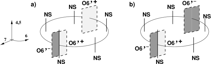
Figure 2: Typical ${\cal N}=1$ brane configurations obtained by introducing O$6^{\prime}$-planes in ${\cal N}=2$ elliptic models with odd number of NS-branes. Notice the fork configuration, where the O$6^{\prime}$-plane changes sign when it crosses the NS-brane. The change of sign is depicted by a change of color. The eight half D6^′-branes stuck on the negatively charged half of the orientifold are not shown in the picture.

The charge of the remaining O$6^{\prime}$-plane can be chosen of either sign, so for a given $N$ there are two possible configurations, which are depicted in figure 2. To give an example of the field theories that are obtained from these brane configurations, let us consider the fork-O$6\,^{\prime}\,{}^{+}$ configuration, figure 2a. The field theory gauge group and ${\cal N}=1$ matter content is

$$\begin{array}[]{ccc}&SO(n_{0})\times\prod_{i=1}^{P}U(n_{i})&\\ Q_{i,i+1}&(\raisebox{-0.5pt}{\hbox{\rule{0.4pt}{6.5pt}\hskip-0.4pt\rule{6.5pt}{0.4pt}\hskip-6.5pt\rule[6.5pt]{6.5pt}{0.4pt}}\rule[6.5pt]{0.4pt}{0.4pt}\hskip-0.4pt\rule{0.4pt}{6.5pt}}_{i},\overline{\raisebox{-0.5pt}{\hbox{\rule{0.4pt}{6.5pt}\hskip-0.4pt\rule{6.5pt}{0.4pt}\hskip-6.5pt\rule[6.5pt]{6.5pt}{0.4pt}}\rule[6.5pt]{0.4pt}{0.4pt}\hskip-0.4pt\rule{0.4pt}{6.5pt}}}_{i+1})&i=0,\ldots,P-1\\ {\tilde{Q}}_{i+1,i}&(\raisebox{-0.5pt}{\hbox{\rule{0.4pt}{6.5pt}\hskip-0.4pt\rule{6.5pt}{0.4pt}\hskip-6.5pt\rule[6.5pt]{6.5pt}{0.4pt}}\rule[6.5pt]{0.4pt}{0.4pt}\hskip-0.4pt\rule{0.4pt}{6.5pt}}_{i+1},\overline{\raisebox{-0.5pt}{\hbox{\rule{0.4pt}{6.5pt}\hskip-0.4pt\rule{6.5pt}{0.4pt}\hskip-6.5pt\rule[6.5pt]{6.5pt}{0.4pt}}\rule[6.5pt]{0.4pt}{0.4pt}\hskip-0.4pt\rule{0.4pt}{6.5pt}}}_{i})&i=0,\ldots,P-1\\ S_{0}&\raisebox{-0.5pt}{\hbox{\rule{0.4pt}{6.5pt}\hskip-0.4pt\rule{6.5pt}{0.4pt}\hskip-6.5pt\rule[6.5pt]{6.5pt}{0.4pt}}\rule[6.5pt]{0.4pt}{0.4pt}\hskip-0.4pt\rule{0.4pt}{6.5pt}}\hskip-0.4pt\raisebox{-0.5pt}{\hbox{\rule{0.4pt}{6.5pt}\hskip-0.4pt\rule{6.5pt}{0.4pt}\hskip-6.5pt\rule[6.5pt]{6.5pt}{0.4pt}}\rule[6.5pt]{0.4pt}{0.4pt}\hskip-0.4pt\rule{0.4pt}{6.5pt}}_{0}&\\ \Phi_{i}&{\rm Adj}_{\;i}&i=1,\ldots,P\\ {\tilde{S}}_{P}&{\overline{\raisebox{-0.5pt}{\hbox{\rule{0.4pt}{6.5pt}\hskip-0.4pt\rule{6.5pt}{0.4pt}\hskip-6.5pt\rule[6.5pt]{6.5pt}{0.4pt}}\rule[6.5pt]{0.4pt}{0.4pt}\hskip-0.4pt\rule{0.4pt}{6.5pt}}\hskip-0.4pt\raisebox{-0.5pt}{\hbox{\rule{0.4pt}{6.5pt}\hskip-0.4pt\rule{6.5pt}{0.4pt}\hskip-6.5pt\rule[6.5pt]{6.5pt}{0.4pt}}\rule[6.5pt]{0.4pt}{0.4pt}\hskip-0.4pt\rule{0.4pt}{6.5pt}}}}_{P}&\\ A_{P}&\raisebox{-3.5pt}{\hbox{\rule{0.4pt}{6.5pt}\hskip-0.4pt\rule{6.5pt}{0.4pt}\hskip-6.5pt\rule[6.5pt]{6.5pt}{0.4pt}}\rule[6.5pt]{0.4pt}{0.4pt}\hskip-0.4pt\rule{0.4pt}{6.5pt}}\hskip-6.9pt\raisebox{3.0pt}{\hbox{\rule{0.4pt}{6.5pt}\hskip-0.4pt\rule{6.5pt}{0.4pt}\hskip-6.5pt\rule[6.5pt]{6.5pt}{0.4pt}}\rule[6.5pt]{0.4pt}{0.4pt}\hskip-0.4pt\rule{0.4pt}{6.5pt}}_{P}&\\ T_{P}^{a}&\raisebox{-0.5pt}{\hbox{\rule{0.4pt}{6.5pt}\hskip-0.4pt\rule{6.5pt}{0.4pt}\hskip-6.5pt\rule[6.5pt]{6.5pt}{0.4pt}}\rule[6.5pt]{0.4pt}{0.4pt}\hskip-0.4pt\rule{0.4pt}{6.5pt}}_{P}&a=1,\ldots,8\end{array}$$ (3.9)

The superpotential is given by

$$W = S_{0}Q_{0,1}{\tilde{Q}_{1,0}}+\sum_{i=1}^{P-1}\,[\,-\Phi_{i}{\tilde{Q}}_{i,i-1}Q_{i-1,i}\;+\;\Phi_{i}Q_{i,i+1}{\tilde{Q}}_{i+1,i}\,]\,+$$ (3.10)

$$-\Phi_{P}{\tilde{Q}}_{P,P-1}Q_{P-1,P}+{\tilde{S}}_{P}T_{P}T_{P}$$

The field theory for the fork-O$6\,^{\prime}\,{}^{-}$ configuration, figure 2b, is obtained by replacing $SO(n_{0})$ by $USp(n_{0})$, and the symmetric representation $S_{0}$ by an antisymmetric $A_{0}$.

3.2 Even number of NS branes, $N=2P$

When the number of NS-branes is even, $N=2P$, there are two possible $\bf Z_{2}$-invariant arrangements of NS branes, depending on whether or not there are NS-branes coinciding with the O$6^{\prime}$-planes.

3.2.1 Models without NS branes on top of the orientifold planes

The configurations contain $P$ pairs of NS-branes related by the $\bf Z_{2}$ symmetry. Since no NS-branes intersects the O6^′-planes, there are no fork configurations and the theories will be non-chiral. As shown in figure 3, there are three possible choices for the signs of the O$6^{\prime}$-planes.

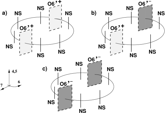
Figure 3: The ${\cal N}=1$ brane configurations with O$6^{\prime}$-planes and an even number of NS-branes, in the case in which no NS-brane coincides with the orientifold planes.

The field theories can be read off directly from the brane picture. For instance, for the O$6\,^{\prime}\,{}^{+}$-O$6\,^{\prime}\,{}^{+}$configuration in figure 3a, we have

$$\begin{array}[]{ccc}&SO(n_{0})\times\prod_{i=1}^{P-1}U(n_{i})\times SO(n_{P})&\\ Q_{i,i+1}&(\raisebox{-0.5pt}{\hbox{\rule{0.4pt}{6.5pt}\hskip-0.4pt\rule{6.5pt}{0.4pt}\hskip-6.5pt\rule[6.5pt]{6.5pt}{0.4pt}}\rule[6.5pt]{0.4pt}{0.4pt}\hskip-0.4pt\rule{0.4pt}{6.5pt}}_{i},\overline{\raisebox{-0.5pt}{\hbox{\rule{0.4pt}{6.5pt}\hskip-0.4pt\rule{6.5pt}{0.4pt}\hskip-6.5pt\rule[6.5pt]{6.5pt}{0.4pt}}\rule[6.5pt]{0.4pt}{0.4pt}\hskip-0.4pt\rule{0.4pt}{6.5pt}}}_{i+1})&i=0,\ldots,P-1\\ {\tilde{Q}}_{i+1,i}&(\raisebox{-0.5pt}{\hbox{\rule{0.4pt}{6.5pt}\hskip-0.4pt\rule{6.5pt}{0.4pt}\hskip-6.5pt\rule[6.5pt]{6.5pt}{0.4pt}}\rule[6.5pt]{0.4pt}{0.4pt}\hskip-0.4pt\rule{0.4pt}{6.5pt}}_{i+1},\overline{\raisebox{-0.5pt}{\hbox{\rule{0.4pt}{6.5pt}\hskip-0.4pt\rule{6.5pt}{0.4pt}\hskip-6.5pt\rule[6.5pt]{6.5pt}{0.4pt}}\rule[6.5pt]{0.4pt}{0.4pt}\hskip-0.4pt\rule{0.4pt}{6.5pt}}}_{i})&i=0,\ldots,P-1\\ S_{0}&\raisebox{-0.5pt}{\hbox{\rule{0.4pt}{6.5pt}\hskip-0.4pt\rule{6.5pt}{0.4pt}\hskip-6.5pt\rule[6.5pt]{6.5pt}{0.4pt}}\rule[6.5pt]{0.4pt}{0.4pt}\hskip-0.4pt\rule{0.4pt}{6.5pt}}\hskip-0.4pt\raisebox{-0.5pt}{\hbox{\rule{0.4pt}{6.5pt}\hskip-0.4pt\rule{6.5pt}{0.4pt}\hskip-6.5pt\rule[6.5pt]{6.5pt}{0.4pt}}\rule[6.5pt]{0.4pt}{0.4pt}\hskip-0.4pt\rule{0.4pt}{6.5pt}}_{\,0}&\\ \Phi_{i}&Adj_{\,i}&i=1,\ldots,P-1\\ S_{P}&\raisebox{-0.5pt}{\hbox{\rule{0.4pt}{6.5pt}\hskip-0.4pt\rule{6.5pt}{0.4pt}\hskip-6.5pt\rule[6.5pt]{6.5pt}{0.4pt}}\rule[6.5pt]{0.4pt}{0.4pt}\hskip-0.4pt\rule{0.4pt}{6.5pt}}\hskip-0.4pt\raisebox{-0.5pt}{\hbox{\rule{0.4pt}{6.5pt}\hskip-0.4pt\rule{6.5pt}{0.4pt}\hskip-6.5pt\rule[6.5pt]{6.5pt}{0.4pt}}\rule[6.5pt]{0.4pt}{0.4pt}\hskip-0.4pt\rule{0.4pt}{6.5pt}}_{P}&\end{array}$$ (3.17)

The superpotential is given by

$$W=S_{0}Q_{0,1}{\tilde{Q}_{1,0}}+\sum_{i=1}^{P-1}\,[\,-\Phi_{i}{\tilde{Q}}_{i,i-1}Q_{i-1,i}\;+\;\Phi_{i}Q_{i,i+1}{\tilde{Q}}_{i+1,i}\,]\,-S_{P}{\tilde{Q}}_{P,P-1}Q_{P-1,P}$$ (3.18)

The field theory corresponding to the O$6\,^{\prime}\,{}^{+}$-O$6\,^{\prime}\,{}^{-}$configuration in figure 3b is obtained from the above one by changing e.g. $SO(n_{0})$ by $USp(n_{0})$ and the symmetric $S_{0}$ by an antisymmetric $A_{0}$. The field theory for the configuration in O$6\,^{\prime}\,{}^{-}$-O$6\,^{\prime}\,{}^{-}$in figure 3c is obtained by changing both orthogonal factors to symplectic ones, and both symmetric representations to antisymmetric ones.

3.2.2 Models with NS branes coinciding with the O$6^{\prime}$-planes

These configurations contain $P-1$ pairs of NS-branes, and two unpaired NS-branes. The latter are stuck at the two O6^′-planes, which are therefore split in halves and give rise to two fork configurations. There are two possible models for a given $N$, shown in figure 4, which only differ in the orientation of the forks in $x^{7}$. We will denote the two relative orientations as ‘antiparallel’ and ‘parallel’.

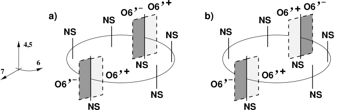
Figure 4: The ${\cal N}=1$ brane configurations with O$6^{\prime}$-planes and an even number of NS branes, in the case with NS branes coinciding with the orientifold planes.

Considering for instance the case of ‘parallel’ forks, the field theory obtained is given by

$$\begin{array}[]{ccc}&\prod_{i=1}^{P}U(n_{i})&\\ Q_{i,i+1}&(\raisebox{-0.5pt}{\hbox{\rule{0.4pt}{6.5pt}\hskip-0.4pt\rule{6.5pt}{0.4pt}\hskip-6.5pt\rule[6.5pt]{6.5pt}{0.4pt}}\rule[6.5pt]{0.4pt}{0.4pt}\hskip-0.4pt\rule{0.4pt}{6.5pt}}_{i},\overline{\raisebox{-0.5pt}{\hbox{\rule{0.4pt}{6.5pt}\hskip-0.4pt\rule{6.5pt}{0.4pt}\hskip-6.5pt\rule[6.5pt]{6.5pt}{0.4pt}}\rule[6.5pt]{0.4pt}{0.4pt}\hskip-0.4pt\rule{0.4pt}{6.5pt}}}_{i+1})&i=1,\ldots,P-1\\ {\tilde{Q}}_{i+1,i}&(\raisebox{-0.5pt}{\hbox{\rule{0.4pt}{6.5pt}\hskip-0.4pt\rule{6.5pt}{0.4pt}\hskip-6.5pt\rule[6.5pt]{6.5pt}{0.4pt}}\rule[6.5pt]{0.4pt}{0.4pt}\hskip-0.4pt\rule{0.4pt}{6.5pt}}_{i+1},\overline{\raisebox{-0.5pt}{\hbox{\rule{0.4pt}{6.5pt}\hskip-0.4pt\rule{6.5pt}{0.4pt}\hskip-6.5pt\rule[6.5pt]{6.5pt}{0.4pt}}\rule[6.5pt]{0.4pt}{0.4pt}\hskip-0.4pt\rule{0.4pt}{6.5pt}}}_{i})&i=1,\ldots,P-1\\ S_{1}&\raisebox{-0.5pt}{\hbox{\rule{0.4pt}{6.5pt}\hskip-0.4pt\rule{6.5pt}{0.4pt}\hskip-6.5pt\rule[6.5pt]{6.5pt}{0.4pt}}\rule[6.5pt]{0.4pt}{0.4pt}\hskip-0.4pt\rule{0.4pt}{6.5pt}}\hskip-0.4pt\raisebox{-0.5pt}{\hbox{\rule{0.4pt}{6.5pt}\hskip-0.4pt\rule{6.5pt}{0.4pt}\hskip-6.5pt\rule[6.5pt]{6.5pt}{0.4pt}}\rule[6.5pt]{0.4pt}{0.4pt}\hskip-0.4pt\rule{0.4pt}{6.5pt}}_{1}&\\ {\tilde{A}}_{1}&\overline{\raisebox{-3.5pt}{\hbox{\rule{0.4pt}{6.5pt}\hskip-0.4pt\rule{6.5pt}{0.4pt}\hskip-6.5pt\rule[6.5pt]{6.5pt}{0.4pt}}\rule[6.5pt]{0.4pt}{0.4pt}\hskip-0.4pt\rule{0.4pt}{6.5pt}}\hskip-6.9pt\raisebox{3.0pt}{\hbox{\rule{0.4pt}{6.5pt}\hskip-0.4pt\rule{6.5pt}{0.4pt}\hskip-6.5pt\rule[6.5pt]{6.5pt}{0.4pt}}\rule[6.5pt]{0.4pt}{0.4pt}\hskip-0.4pt\rule{0.4pt}{6.5pt}}}_{\,1}&\\ {\tilde{T}}_{1,a}&\overline{\raisebox{-0.5pt}{\hbox{\rule{0.4pt}{6.5pt}\hskip-0.4pt\rule{6.5pt}{0.4pt}\hskip-6.5pt\rule[6.5pt]{6.5pt}{0.4pt}}\rule[6.5pt]{0.4pt}{0.4pt}\hskip-0.4pt\rule{0.4pt}{6.5pt}}}_{1}&a=1,\ldots,8\\ \Phi_{i}&{\rm Adj}_{i}&i=1,\ldots,P\\ {\tilde{S}}_{P}&{\overline{\raisebox{-0.5pt}{\hbox{\rule{0.4pt}{6.5pt}\hskip-0.4pt\rule{6.5pt}{0.4pt}\hskip-6.5pt\rule[6.5pt]{6.5pt}{0.4pt}}\rule[6.5pt]{0.4pt}{0.4pt}\hskip-0.4pt\rule{0.4pt}{6.5pt}}\hskip-0.4pt\raisebox{-0.5pt}{\hbox{\rule{0.4pt}{6.5pt}\hskip-0.4pt\rule{6.5pt}{0.4pt}\hskip-6.5pt\rule[6.5pt]{6.5pt}{0.4pt}}\rule[6.5pt]{0.4pt}{0.4pt}\hskip-0.4pt\rule{0.4pt}{6.5pt}}}}_{P}&\\ A_{P}&\raisebox{-3.5pt}{\hbox{\rule{0.4pt}{6.5pt}\hskip-0.4pt\rule{6.5pt}{0.4pt}\hskip-6.5pt\rule[6.5pt]{6.5pt}{0.4pt}}\rule[6.5pt]{0.4pt}{0.4pt}\hskip-0.4pt\rule{0.4pt}{6.5pt}}\hskip-6.9pt\raisebox{3.0pt}{\hbox{\rule{0.4pt}{6.5pt}\hskip-0.4pt\rule{6.5pt}{0.4pt}\hskip-6.5pt\rule[6.5pt]{6.5pt}{0.4pt}}\rule[6.5pt]{0.4pt}{0.4pt}\hskip-0.4pt\rule{0.4pt}{6.5pt}}_{P}&\\ T_{P,a}&\raisebox{-0.5pt}{\hbox{\rule{0.4pt}{6.5pt}\hskip-0.4pt\rule{6.5pt}{0.4pt}\hskip-6.5pt\rule[6.5pt]{6.5pt}{0.4pt}}\rule[6.5pt]{0.4pt}{0.4pt}\hskip-0.4pt\rule{0.4pt}{6.5pt}}_{P}&a=1,\ldots,8\\ \end{array}$$ (3.29)

The superpotential is given by

$$W= S_{1}{\tilde{T}}_{1}{\tilde{T}}_{1}+\Phi_{1}Q_{1,2}{\tilde{Q}}_{2,1}+\sum_{i=2}^{P-1}\;[\,-\Phi_{i}{\tilde{Q}}_{i,i-1}Q_{i-1,i}\;+\;\Phi_{i}Q_{i,i+1}{\tilde{Q}}_{i+1,i}\,]\,+$$ (3.30)

$$-\Phi_{P}{\tilde{Q}}_{P,P-1}Q_{P-1,P}+{\tilde{S}}_{P}T_{P}T_{P}$$

Changing the orientation of a fork simply conjugates the corresponding representations $S$, ${\tilde{A}}$ and ${\tilde{T}}$. Even though the difference between the two configurations may seem rather subtle, the models are different and should be treated as such. For instance, notice the particular case of having only two NS branes, where one of the configurations is chiral and the other is non-chiral (even though there is chiral matter localized at points in the circle).

We have completed the classification of type IIA configurations obtained by adding O6^′-planes to the ${\cal N}=2$ elliptic models. In the following subsection we construct the same field theories in a T-dual IIB singularity picture.

4 The type IIB orientifold construction

In this section we provide a type IIB T-dual construction of the field theories studied in the previous section, in terms of D3-branes probing certain orientifolds of $\bf C^{2}/\bf Z_{N}$. We will show that the classification of the different orientifold projections reproduces the classification of type IIA models. This T-duality map gives a type IIB singularity realization of the different phenomena observed in the IIA brane construction, giving rise to chiral symmetries and chiral matter. These features of the field theory arise in a natural fashion in the orientifold construction.

Our goal in this section is to provide a construction of these field theories in the type IIB side. Since in the type IIA setup the models were obtained by introducing orientifold planes in a ${\cal N}=2$ elliptic model, we expect the type IIB realization to correspond to an orientifold projection on the system of D3-branes at an orbifold singularity $\bf C^{2}/\bf Z_{N}\times\bf C$, with the generator $\theta$ of $\bf Z_{N}$ acting as

$$(z_{1},z_{2},z_{3})\rightarrow(e^{2\pi i/N}z_{1},e^{-2\pi i/N}z_{2},z_{3})$$ (4.1)

A difference with the ${\cal N}=2$ orientifold models studied in [39] is that in our case the orientifold projection must break half of the supersymmetries, yielding ${\cal N}=1$ field theories on the D3-brane world-volume. Thus, a suitable orientation reversing element is $\Omega_{1}\equiv\Omega(-1)^{F_{L}}R_{1}$ (rather than the ${\cal N}=2$ preserving $\Omega_{3}\equiv\Omega(-1)^{F_{L}}R_{3}$). Here $R_{i}$ changes the sign of the complex coordinate $z_{i}$, leaving the others invariant.

Our proposal is that the field theories will be realized in the world-volume of a system of D3-branes at the orientifold singularities obtained by modding the orbifold (4.1) by the world-sheet orientation reversing action $\Omega_{1}$. This is actually suggested by T-dualizing the IIA configurations along $x^{6}$ (for a detailed description of this T-duality in a particular case, see [30]). Namely, the NS-branes along 012345 transform into the orbifold above (if we identify the 45, 67, 89 planes with, say, the $z_{3}$, $z_{2}$, $z_{1}$ complex planes), the D4-branes turn into D3-brane probes, and the type IIA orientifold action $\Omega(-1)^{F_{L}}I_{689}$ transforms into $\Omega(-1)^{F_{L}}R_{1}$.

In the following section we turn to the classification and explicit construction of these type IIB orientifolds. We show that the field theories on the D3-branes actually reproduce the field theories in the previous section. Moreover, we discuss how the orientifold structure on the IIA side is neatly encoded in the structure of the IIB orientifold group. This strongly supports the T-duality argument sketched above, and also provides a singularity realization of the fork configurations yielding chiral matter. We also mention that the consistency conditions of the IIB orientifolds (cancellation of twisted tadpoles) imply the cancellation of gauge anomalies in the D3-brane world-volume theory (the corresponding tadpole computations are however postponed until Section 5). These models provide an interesting realization of how an inconsistency in a background is detected as an anomaly on a D-brane probe.

4.1 Odd order case, $N=2P+1$

4.1.1 Construction

Let us consider the case where the orientifold group is ${\bf Z_{N}}+\Omega_{1}{\bf Z_{N}}$, i.e. the orientifold projection has the structure

$$(1+\theta+\theta^{2}+\cdots+\theta^{N-1})(1+\Omega_{1})$$ (4.2)

where $\Omega_{1}\equiv\Omega(-1)^{F_{L}}R_{1}$

We will consider the following choice of Chan-Paton matrices for the D3-branes.

$$\gamma_{\theta,3}\,=\,{\rm diag}(1_{n_{0}},e^{2\pi i\frac{1}{N}}1_{n_{1}},\ldots,e^{2\pi i\frac{P}{N}}1_{n_{P}},e^{2\pi i\frac{P+1}{N}}1_{n_{P}},\ldots,e^{2\pi i\frac{2P}{N}}1_{n_{1}})$$ (4.3)

$${\footnotesize\gamma_{\Omega_{1},3}=\pmatrix{1_{n_{0}}&&&&&&\cr&&&&&&1_{n_{1}}\cr&&&&&\cdots&\cr&&&&1_{n_{P}}&&\cr&&&1_{n_{P}}&&&\cr&&\cdots&&&&\cr&1_{n_{1}}&&&&&\cr}\;{\rm or}\;\gamma_{\Omega_{1},3}=\pmatrix{\varepsilon_{n_{0}}&&&&&&\cr&&&&&&1_{n_{1}}\cr&&&&&\cdots&\cr&&&&1_{n_{P}}&&\cr&&&-1_{n_{P}}&&&\cr&&\cdots&&&&\cr&-1_{n_{1}}&&&&&\cr}}$$

where $\varepsilon_{n_{0}}=\pmatrix{0&1_{n_{0}/2}\cr-1_{n_{0}/2}&0}$. These matrices satisfy the group law and all algebraic consistency conditions imposed by the structure of the orientifold group. The two possibilities for $\gamma_{\Omega_{1},3}$, symmetric or antisymmetric, correspond to choosing the $SO$ or $Sp$ orientifold projection on the D3-branes.

It is a simple exercise to compute the 3-3 spectrum that arises from the projections imposed by the above matrices. For instance, for the $SO$ projection, we obtain the following gauge group and matter content (we have already taken into account the disappearance of the $U(1)$ factors)

$$SO(n_{0})\times SU(n_{1})\times SU(n_{P})$$

$$\sum_{i=0}^{P-1}\;[\;(\raisebox{-0.5pt}{\hbox{\rule{0.4pt}{6.5pt}\hskip-0.4pt\rule{6.5pt}{0.4pt}\hskip-6.5pt\rule[6.5pt]{6.5pt}{0.4pt}}\rule[6.5pt]{0.4pt}{0.4pt}\hskip-0.4pt\rule{0.4pt}{6.5pt}}_{i},\overline{\raisebox{-0.5pt}{\hbox{\rule{0.4pt}{6.5pt}\hskip-0.4pt\rule{6.5pt}{0.4pt}\hskip-6.5pt\rule[6.5pt]{6.5pt}{0.4pt}}\rule[6.5pt]{0.4pt}{0.4pt}\hskip-0.4pt\rule{0.4pt}{6.5pt}}}_{i+1})+(\overline{\raisebox{-0.5pt}{\hbox{\rule{0.4pt}{6.5pt}\hskip-0.4pt\rule{6.5pt}{0.4pt}\hskip-6.5pt\rule[6.5pt]{6.5pt}{0.4pt}}\rule[6.5pt]{0.4pt}{0.4pt}\hskip-0.4pt\rule{0.4pt}{6.5pt}}}_{i},\raisebox{-0.5pt}{\hbox{\rule{0.4pt}{6.5pt}\hskip-0.4pt\rule{6.5pt}{0.4pt}\hskip-6.5pt\rule[6.5pt]{6.5pt}{0.4pt}}\rule[6.5pt]{0.4pt}{0.4pt}\hskip-0.4pt\rule{0.4pt}{6.5pt}}_{i+1})\;]\;+\raisebox{-3.5pt}{\hbox{\rule{0.4pt}{6.5pt}\hskip-0.4pt\rule{6.5pt}{0.4pt}\hskip-6.5pt\rule[6.5pt]{6.5pt}{0.4pt}}\rule[6.5pt]{0.4pt}{0.4pt}\hskip-0.4pt\rule{0.4pt}{6.5pt}}\hskip-6.9pt\raisebox{3.0pt}{\hbox{\rule{0.4pt}{6.5pt}\hskip-0.4pt\rule{6.5pt}{0.4pt}\hskip-6.5pt\rule[6.5pt]{6.5pt}{0.4pt}}\rule[6.5pt]{0.4pt}{0.4pt}\hskip-0.4pt\rule{0.4pt}{6.5pt}}_{P}+{\overline{\raisebox{-0.5pt}{\hbox{\rule{0.4pt}{6.5pt}\hskip-0.4pt\rule{6.5pt}{0.4pt}\hskip-6.5pt\rule[6.5pt]{6.5pt}{0.4pt}}\rule[6.5pt]{0.4pt}{0.4pt}\hskip-0.4pt\rule{0.4pt}{6.5pt}}\hskip-0.4pt\raisebox{-0.5pt}{\hbox{\rule{0.4pt}{6.5pt}\hskip-0.4pt\rule{6.5pt}{0.4pt}\hskip-6.5pt\rule[6.5pt]{6.5pt}{0.4pt}}\rule[6.5pt]{0.4pt}{0.4pt}\hskip-0.4pt\rule{0.4pt}{6.5pt}}}}_{P}+\raisebox{-0.5pt}{\hbox{\rule{0.4pt}{6.5pt}\hskip-0.4pt\rule{6.5pt}{0.4pt}\hskip-6.5pt\rule[6.5pt]{6.5pt}{0.4pt}}\rule[6.5pt]{0.4pt}{0.4pt}\hskip-0.4pt\rule{0.4pt}{6.5pt}}\hskip-0.4pt\raisebox{-0.5pt}{\hbox{\rule{0.4pt}{6.5pt}\hskip-0.4pt\rule{6.5pt}{0.4pt}\hskip-6.5pt\rule[6.5pt]{6.5pt}{0.4pt}}\rule[6.5pt]{0.4pt}{0.4pt}\hskip-0.4pt\rule{0.4pt}{6.5pt}}_{0}+\sum_{i=1}^{P}{\rm Adj}_{\,i}$$ (4.4)

It reproduces the spectrum (3.9) of the field theory corresponding to the IIA configuration figure 2a, studied in section 3. This was expected, since the T-duality argument implies the order of the orbifold group matches the number of NS-branes in the IIA picture. The superpotential interactions in the IIB orientifold also reproduce the IIA result (3.10).

Notice that the spectrum above is actually missing some of the states in the IIA brane configuration, namely the eight fundamental flavours arising from the half D6^′-branes in the fork. The solution to this issue comes from the fact that the IIB orientifold above is not consistent yet, since it contains non-cancelled tadpoles (see section 5.1). This inconsistency is manifest in the field theory, since the $SU(n_{P})$ factor is anomalous. The tadpoles can be cancelled by introducing D7 branes. The minimal choice to cancel the tadpoles (see eq. (5.22)) is to place eight D7₂-branes with Chan-Paton matrices

$$\gamma_{\theta,{7_{2}}}=-{\bf 1}_{8}\quad;\quad\gamma_{\Omega_{1},7_{2}}={\bf 1}_{8}$$ (4.5)

The 3-7₂ spectrum yields the 8 fundamentals of $U(n_{P})$ required to cancel the anomalies and complete the matching with the spectrum obtained from the type IIA brane configuration. The interactions between 3-7₂ states and 3-3 states (more concretely, those associated to the second complex plane) in the orientifold provides the coupling between the fundamentals and symmetric of $SU(n_{P})$. Also, the $SO(8)$ symmetry on the D7₂-brane world-volume agrees with the $SO(8)$ symmetry of the half D6^′-branes in the IIA picture. The fact that whole D7₂-branes are T-dual to half D6^′-branes confirms our expectations from the analysis in section 2. Further evidence is provided in section 5.1, where we study models with more complicated choices of D7-brane Chan-Paton matrices, and their interpretation in terms of type IIA picture.

Another interesting feature is that the geometry of the type IIB orientifold encodes the change of sign of the IIA O6^′-plane. In figure 2a, for negative values of $x^{7}$ both O6^′-planes are positively charged, while for positive values of $x^{7}$ their charges are opposite. This translates into different behaviours of the IIB orientifold projection with respect to the two complex planes in $\bf C^{2}/\bf Z_{N}$. In fact, the orientifold group (4.2) contains the element $\Omega(-1)^{F_{L}}R_{1}$, and the model contains an O7⁺-plane wrapped along $z_{2}$. This is the T-dual to the two positively charged O6^′-planes in the positive $x^{7}$ region in the IIA construction. On the other hand, the IIB orientifold group does not contain $\Omega(-1)^{F_{L}}R_{2}$, so there is no RR charge along the complex plane$z_{1}$. This corresponds to the fact that the O6^′-plane charges compensate in the negative $x^{7}$ region in the IIA picture.

The orientifold obtained with the antisymmetric $\gamma_{\Omega_{1},3}$ can be analyzed analogously. It provides a construction of the field theory corresponding to the IIA configuration in figure 2b.

As a final comment, let us mention that there is another consistent structure for the orientifold group, given by

$$(1+\theta+\theta^{2}+\cdots+\theta^{N-1})(1+\alpha\Omega_{1}),$$ (4.6)

with $\alpha:(z_{1},z_{2},z_{3})\to(e^{\pi i/N}z_{1},e^{-\pi i/N}z_{2},z_{3})$. However, it does not provide new models. In order to see that, recall that $\theta^{P}\alpha=R_{1}R_{2}$, so the projection above is equivalent to a projection using $\Omega_{2}\equiv\Omega(-1)^{F_{L}}R_{2}$ (without $\alpha$), which is equivalent to the one above.

4.1.2 Comparison with ${\cal N}=2$ models

The ${\cal N}=1$ orientifolds just constructed differ from the ${\cal N}=2$ models of [39] only in the use of $\Omega_{1}$ instead of $\Omega_{3}$ as the orientifold action. This apparently innocent change has nevertheless a dramatic effect in the field theory. In particular, it is responsible for the appearance of the fork structure, and consequently, of chiral matter. In what follows we compare both projections, and discuss how the $\Omega_{1}$ orientifold yields the fork matter content. The projections are given in the following table

	${\cal N}=2$ projection	${\cal N}=1$ projection
Vector mult:	$\quad V=-\gamma_{\Omega_{3}}V^{T}\gamma_{\Omega_{3}}^{-1}\quad$	$\quad V=-\gamma_{\Omega_{1}}V^{T}\gamma_{\Omega_{1}}^{-1}\quad$
Ch.mult. $Z_{1}$:	$\quad Z_{1}=+\gamma_{\Omega_{3}}Z_{1}^{T}\gamma_{\Omega_{3}}^{-1}\quad$	$\quad Z_{1}=-\gamma_{\Omega_{1}}Z_{1}^{T}\gamma_{\Omega_{1}}^{-1}\quad$
Ch.mult. $Z_{2}$:	$\quad Z_{2}=+\gamma_{\Omega_{3}}Z_{2}^{T}\gamma_{\Omega_{3}}^{-1}\quad$	$\quad Z_{2}=+\gamma_{\Omega_{1}}Z_{2}^{T}\gamma_{\Omega_{1}}^{-1}\quad$
Ch.mult. $Z_{3}$:	$\quad Z_{3}=-\gamma_{\Omega_{3}}Z_{3}^{T}\gamma_{\Omega_{3}}^{-1}\quad$	$\quad Z_{3}=+\gamma_{\Omega_{1}}Z_{3}^{T}\gamma_{\Omega_{1}}^{-1}\quad$

Recall that before the orientifold projection, the ${\cal N}=1$ multiplets $V$ and $Z_{3}$ pair up to form ${\cal N}=2$ vector multiplets. Analogously, the chiral multiplets $Z_{1}$, $Z_{2}$ form ${\cal N}=2$ hypermultiplets. This ${\cal N}=2$ structure is preserved by the projection $\Omega_{3}$, while the projection $\Omega_{1}$ introduces relative signs that break the structure of ${\cal N}=2$ multiplets. The effects of these signs are most manifest in two sectors of the field theory which we now analyze:

Consider first the two ${\cal N}=1$ multiplets $V$, $Z_{3}$ in the ${\cal N}=2$ vector multiplet in the adjoint of $U(n_{0})$ in the orbifold theory, before the orientifold projection. From the above equations (for a specific choice of $\gamma_{\Omega_{i}}$, say, symmetric), we see $\Omega_{3}$ projects both multiplets to adjoints of $SO(n_{0})$, in agreement with ${\cal N}=2$ supersymmetry. On the other hand, $\Omega_{1}$ projects the ${\cal N}=1$ vector multiplet $V$ to the adjoint of $SO(n_{0})$, and the chiral multiplet $Z_{3}$ to the symmetric representation. This nicely parallels the results in the IIA brane configuration [12], where $n_{0}$ D4-branes stretched between two NS-branes, in the presence of an O6⁺-plane give rise to a $SO(n_{0})$ gauge group with one antisymmetric chiral multiplet [42], and in the presence of an O6${}^{\prime}\,{}^{+}$-plane give a $SO(n_{0})$ gauge group and one symmetric chiral multiplet.

Now we consider the projection at the other end of the chain of gauge factors, and look at what kind of two-index representations of $U(n_{P})$ are obtained. For the projections $\Omega_{3}$, we obtain one chiral multiplet in the symmetric and one in the conjugate symmetric representation, in agreement with ${\cal N}=2$ supersymmetry. For the projection $\Omega_{1}$ we obtain one chiral multiplet in the antisymmetric and one in the conjugate symmetric representation. This is basically the fork configuration that appears in the T dual IIA configuration.

As mentioned above, the spectrum in the fork configuration also includes chiral flavours coming from eight half D6^′-branes, required to conserve the RR charge. The ${\cal N}=2$ IIA configuration, however, does not require the presence of D6-branes for consistency. These features are also reproduced in the IIB orientifold construction, as is revealed by studying the dependence of the Klein bottle tadpoles with the volume $V_{3}$ of the complex plane $z_{3}$, which we momentarily imagine to be compact. The projection $\Omega_{3}$ allows winding states in the direction $z_{3}$, which give (after Poisson resumming) a tadpole inversely proportional to $V_{3}$. The tadpole vanishes in the non-compact limit, and the model is consistent without the introduction of D7-branes. The projection $\Omega_{1}$, however, projects out winding states and allows for momentum states. These generate a tadpole proportional to $V_{3}$, which does not vanish in the non-compact limit, and must be cancelled by a suitable set of D7-branes. These provide the fundamental flavours required to complete the fork spectrum in the D3-brane field theory.

4.2 Even order case, $N=2P$

When the order of the orbifold action is even, the group contains a $\bf Z_{2}$ twist, $\theta^{P}$. The orientifold action on the closed string exchanges oppositely twisted sectors [43], and so maps the $\bf Z_{2}$ twisted sector to itself. There is an arbitrary choice of sign in this map, which determines the symmetry of the NS-NS and R-R states that survive the orientifold projection. By open-closed duality, the choice of sign imposes a constraint on the Chan-Paton matrices which act on the open strings, and determines the vector structure of the gauge bundle on the corresponding D-branes (for further details see [44, 43, 45]). For instance, for D7₁-branes we have

$$\gamma_{\theta^{P},7_{1}}=\mp\gamma_{\Omega_{1},7_{1}}\gamma_{\theta^{P},7_{1}}^{T}\gamma_{\Omega_{1},7_{1}}^{-1}$$ (4.7)

with the upper (lower) sign when the $\bf Z_{2}$ RR twisted states surviving the orientifold projection are antisymmetric (symmetric) combinations of left and right movers . These two cases correspond to ${\rm Tr\,}\gamma_{\theta^{N},3}=\pm 1$, respectively, so we will use this fact to refer to both kinds of models.

4.2.1 Models with ${\rm Tr\,}\gamma_{\theta^{N},3}=+1$

There are two different structures for the orientifold group. Consider first the orientifold projection

$$(1+\theta+\theta^{2}+\cdots+\theta^{N-1})(1+\Omega_{1})$$ (4.8)

The Chan-Paton matrices for the D3 branes are

$$\gamma_{\theta,3} = {\rm diag\,}(1_{n_{0}},e^{2\pi i\frac{1}{N}}1_{n_{1}},\cdots,e^{2\pi i\frac{P-1}{N}}1_{n_{P-1}},e^{2\pi i\frac{P}{N}}1_{n_{P}},e^{2\pi i\frac{P+1}{N}}1_{n_{P-1}},\ldots,e^{2\pi i\frac{2P-1}{N}}1_{n_{1}})$$

$$\gamma_{\Omega_{1},3} = {\footnotesize\left(\begin{array}[]{cccccccc}1_{n_{0}}&&&&&&&\\ &&&&&&&1_{n_{1}}\\ &&&&&&\cdots&\\ &&&&&1_{n_{P-1}}&&\\ &&&&1_{n_{P}}&&&\\ &&&1_{n_{P-1}}&&&&\\ &&\cdots&&&&&\\ &1_{n_{1}}&&&&&&\end{array}\right)}$$ (4.17)

These matrices satisfy all algebraic consistency conditions. The corresponding 3-3 spectrum is

$$SO(n_{0})\times SU(n_{1})\times\ldots\times SU(n_{P-1})\times SO(n_{P})$$

$$\sum_{i=0}^{P-1}\;[\;(\raisebox{-0.5pt}{\hbox{\rule{0.4pt}{6.5pt}\hskip-0.4pt\rule{6.5pt}{0.4pt}\hskip-6.5pt\rule[6.5pt]{6.5pt}{0.4pt}}\rule[6.5pt]{0.4pt}{0.4pt}\hskip-0.4pt\rule{0.4pt}{6.5pt}}_{i},\overline{\raisebox{-0.5pt}{\hbox{\rule{0.4pt}{6.5pt}\hskip-0.4pt\rule{6.5pt}{0.4pt}\hskip-6.5pt\rule[6.5pt]{6.5pt}{0.4pt}}\rule[6.5pt]{0.4pt}{0.4pt}\hskip-0.4pt\rule{0.4pt}{6.5pt}}}_{i+1})+(\overline{\raisebox{-0.5pt}{\hbox{\rule{0.4pt}{6.5pt}\hskip-0.4pt\rule{6.5pt}{0.4pt}\hskip-6.5pt\rule[6.5pt]{6.5pt}{0.4pt}}\rule[6.5pt]{0.4pt}{0.4pt}\hskip-0.4pt\rule{0.4pt}{6.5pt}}}_{i},\raisebox{-0.5pt}{\hbox{\rule{0.4pt}{6.5pt}\hskip-0.4pt\rule{6.5pt}{0.4pt}\hskip-6.5pt\rule[6.5pt]{6.5pt}{0.4pt}}\rule[6.5pt]{0.4pt}{0.4pt}\hskip-0.4pt\rule{0.4pt}{6.5pt}}_{i+1})\;]\;+\raisebox{-0.5pt}{\hbox{\rule{0.4pt}{6.5pt}\hskip-0.4pt\rule{6.5pt}{0.4pt}\hskip-6.5pt\rule[6.5pt]{6.5pt}{0.4pt}}\rule[6.5pt]{0.4pt}{0.4pt}\hskip-0.4pt\rule{0.4pt}{6.5pt}}\hskip-0.4pt\raisebox{-0.5pt}{\hbox{\rule{0.4pt}{6.5pt}\hskip-0.4pt\rule{6.5pt}{0.4pt}\hskip-6.5pt\rule[6.5pt]{6.5pt}{0.4pt}}\rule[6.5pt]{0.4pt}{0.4pt}\hskip-0.4pt\rule{0.4pt}{6.5pt}}_{0}+\sum_{i=1}^{P-1}{\rm Adj}_{\,i}+\raisebox{-0.5pt}{\hbox{\rule{0.4pt}{6.5pt}\hskip-0.4pt\rule{6.5pt}{0.4pt}\hskip-6.5pt\rule[6.5pt]{6.5pt}{0.4pt}}\rule[6.5pt]{0.4pt}{0.4pt}\hskip-0.4pt\rule{0.4pt}{6.5pt}}\hskip-0.4pt\raisebox{-0.5pt}{\hbox{\rule{0.4pt}{6.5pt}\hskip-0.4pt\rule{6.5pt}{0.4pt}\hskip-6.5pt\rule[6.5pt]{6.5pt}{0.4pt}}\rule[6.5pt]{0.4pt}{0.4pt}\hskip-0.4pt\rule{0.4pt}{6.5pt}}_{P}$$ (4.18)

This reproduces the spectrum of the field theory (3.17) corresponding to the IIA configuration 3a, studied in Section 3. The superpotential interactions (3.18) are also reproduced in the orientifold. The field theory corresponding to the O$6\,^{\prime}\,{}^{-}$-O$6\,^{\prime}\,{}^{-}$IIA brane configuration, figure 3c, is reproduced by an analogous IIB orientifold using an antisymmetric version for $\gamma_{\Omega_{1}}$.

In these models, the consistency of the IIA brane configuration without D6^′-branes suggests that the type IIB orientifold must be consistent without the addition of D7-branes. In fact, this is confirmed by a computation of the Klein bottle tadpoles, which are found to vanish (see section 5.2.1).

Notice that the orientifold group (4.8) contains both the elements $\Omega(-1)^{F_{L}}R_{1}$ and $\Omega(-1)^{F_{L}}R_{2}$. Therefore, there is RR charge along the complex planes parametrized by $z_{1}$ and $z_{2}$. Under the T-duality, this implies that the IIA configuration contains identically charged upper half O6^′-planes, as well as identically charged lower half O6^′-planes. This is indeed the case for our candidate T-dual IIA models.

There is another possibility for the orientifold group

$$(1+\theta+\theta^{2}+\cdots+\theta^{N-1})(1+\alpha\Omega_{1})$$ (4.19)

with $\alpha:(z_{1},z_{2},z_{3})\to(e^{\pi i/N}z_{1},e^{-\pi i/N}z_{2},z_{3})$. As we show below, this structure provides new models. Let us consider the following D3-brane Chan-Paton matrices

$$\gamma_{\theta,3} = {\rm diag}(1_{n_{0}},e^{2\pi i\frac{1}{N}}1_{n_{1}},\ldots,e^{2\pi i\frac{P-1}{N}}1_{n_{P-1}},e^{2\pi i\frac{P}{N}}1_{n_{P}},e^{2\pi i\frac{P+1}{N}}1_{n_{P-1}},\ldots,e^{2\pi i\frac{2P-1}{N}}1_{n_{1}})$$

$$\gamma_{\alpha\Omega_{1},3} = {\scriptsize\pmatrix{1_{n_{0}}&&&&&&&\cr&&&&&&&\alpha 1_{n_{1}}\cr&&&&&&\cdots&\cr&&&&&\alpha^{P-1}1_{n_{P-1}}&&\cr&&&&\alpha^{P}\varepsilon_{n_{P}}&&&\cr&&&\alpha^{-(P-1)}1_{n_{P-1}}&&&&\cr&&\cdots&&&&&\cr&\alpha^{-1}1_{n_{1}}&&&&&&\cr}}$$ (4.20)

where $\alpha=e^{2\pi i\over{2N}}$. These matrices satisfy the group law and all algebraic consistency conditions. The spectrum of massless 3-3 states is

$$SO(n_{0})\times SU(n_{1})\times\ldots\times SU(n_{P-1})\times USp(n_{P})$$

$$\sum_{i=0}^{P-1}\;[\;(\raisebox{-0.5pt}{\hbox{\rule{0.4pt}{6.5pt}\hskip-0.4pt\rule{6.5pt}{0.4pt}\hskip-6.5pt\rule[6.5pt]{6.5pt}{0.4pt}}\rule[6.5pt]{0.4pt}{0.4pt}\hskip-0.4pt\rule{0.4pt}{6.5pt}}_{i},\overline{\raisebox{-0.5pt}{\hbox{\rule{0.4pt}{6.5pt}\hskip-0.4pt\rule{6.5pt}{0.4pt}\hskip-6.5pt\rule[6.5pt]{6.5pt}{0.4pt}}\rule[6.5pt]{0.4pt}{0.4pt}\hskip-0.4pt\rule{0.4pt}{6.5pt}}}_{i+1})+(\overline{\raisebox{-0.5pt}{\hbox{\rule{0.4pt}{6.5pt}\hskip-0.4pt\rule{6.5pt}{0.4pt}\hskip-6.5pt\rule[6.5pt]{6.5pt}{0.4pt}}\rule[6.5pt]{0.4pt}{0.4pt}\hskip-0.4pt\rule{0.4pt}{6.5pt}}}_{i},\raisebox{-0.5pt}{\hbox{\rule{0.4pt}{6.5pt}\hskip-0.4pt\rule{6.5pt}{0.4pt}\hskip-6.5pt\rule[6.5pt]{6.5pt}{0.4pt}}\rule[6.5pt]{0.4pt}{0.4pt}\hskip-0.4pt\rule{0.4pt}{6.5pt}}_{i+1})\;]\;+\raisebox{-0.5pt}{\hbox{\rule{0.4pt}{6.5pt}\hskip-0.4pt\rule{6.5pt}{0.4pt}\hskip-6.5pt\rule[6.5pt]{6.5pt}{0.4pt}}\rule[6.5pt]{0.4pt}{0.4pt}\hskip-0.4pt\rule{0.4pt}{6.5pt}}\hskip-0.4pt\raisebox{-0.5pt}{\hbox{\rule{0.4pt}{6.5pt}\hskip-0.4pt\rule{6.5pt}{0.4pt}\hskip-6.5pt\rule[6.5pt]{6.5pt}{0.4pt}}\rule[6.5pt]{0.4pt}{0.4pt}\hskip-0.4pt\rule{0.4pt}{6.5pt}}_{0}+\sum_{i=1}^{P-1}{\rm Adj}_{\,i}+\raisebox{-3.5pt}{\hbox{\rule{0.4pt}{6.5pt}\hskip-0.4pt\rule{6.5pt}{0.4pt}\hskip-6.5pt\rule[6.5pt]{6.5pt}{0.4pt}}\rule[6.5pt]{0.4pt}{0.4pt}\hskip-0.4pt\rule{0.4pt}{6.5pt}}\hskip-6.9pt\raisebox{3.0pt}{\hbox{\rule{0.4pt}{6.5pt}\hskip-0.4pt\rule{6.5pt}{0.4pt}\hskip-6.5pt\rule[6.5pt]{6.5pt}{0.4pt}}\rule[6.5pt]{0.4pt}{0.4pt}\hskip-0.4pt\rule{0.4pt}{6.5pt}}_{P}$$ (4.21)

and reproduces the complete field theory spectrum and interactions of the IIA configuration in figure 3b. A nice feature of the type IIB orientifold we have constructed is that the matrix $\gamma_{\alpha\Omega_{1}}$ is rather unique, neither symmetric nor antisymmetric. The fact that this orientifold group structure provides only one class of models agrees with the type IIA construction, where the O$6\,^{\prime}\,{}^{+}$-O$6\,^{\prime}\,{}^{-}$and O$6\,^{\prime}\,{}^{-}$-O$6\,^{\prime}\,{}^{+}$configurations are equivalent. To complete the discussion, let us mention that all dangerous tadpoles vanish in this model (see section 5.2.1), so it is consistent not to include D7-branes.

Finally, let us mention that the orientifold group (4.19) contains neither $\Omega(-1)^{F_{L}}R_{1}$ nor $\Omega(-1)^{F_{L}}R_{2}$, and therefore there is no RR charge along the complex planes in $\bf C^{2}/\bf Z_{N}$. This suggests that the O6^′-plane charges in the T-dual type IIA configuration will cancel both in the positive and in the negative $x^{7}$ regions, as indeed happens for the model in figure 3b.

4.2.2 Models with ${\rm Tr\,}\gamma_{\theta^{N},3}=-1$

As in the theories in the previous subsection, there are two possible choices for the orientifold group. Let us start by considering

$$(1+\theta+\theta^{2}+\cdots+\theta^{N-1})(1+\Omega_{1})$$ (4.22)

We take the following Chan-Paton matrices for the D3 branes

$$\gamma_{\theta,3}={\rm diag\,}(e^{\pi i\frac{1}{N}}1_{n_{1}},e^{\pi i\frac{3}{N}}1_{n_{2}},\cdots,e^{\pi i\frac{2P-1}{N}}1_{n_{P}},e^{\pi i\frac{2P+1}{N}}1_{n_{P}},\cdots,e^{\pi i\frac{4P-3}{N}}1_{n_{2}},e^{\pi i\frac{4P-1}{N}}1_{n_{1}})\quad\quad$$ (4.23)

$$\gamma_{\Omega_{1},3}={\scriptsize\left(\begin{array}[]{cccccccc}&&&&&&&1_{n_{1}}\\ &&&&&&1_{n_{2}}&\\ &&&&&\cdots&&\\ &&&&1_{n_{P}}&&&\\ &&&1_{n_{P}}&&&&\\ &&\cdots&&&&&\\ &1_{n_{2}}&&&&&&\\ 1_{n_{1}}&&&&&&&\end{array}\right)}$$ (4.32)

(In this case using an antisymmetric version of $\gamma_{\Omega_{1}}$ does not produce new models). The matrices satisfy all algebraic consistency conditions. The 3-3 spectrum is

$$SU(n_{1})\times\ldots\times SU(n_{P})$$

$$\overline{\raisebox{-3.5pt}{\hbox{\rule{0.4pt}{6.5pt}\hskip-0.4pt\rule{6.5pt}{0.4pt}\hskip-6.5pt\rule[6.5pt]{6.5pt}{0.4pt}}\rule[6.5pt]{0.4pt}{0.4pt}\hskip-0.4pt\rule{0.4pt}{6.5pt}}\hskip-6.9pt\raisebox{3.0pt}{\hbox{\rule{0.4pt}{6.5pt}\hskip-0.4pt\rule{6.5pt}{0.4pt}\hskip-6.5pt\rule[6.5pt]{6.5pt}{0.4pt}}\rule[6.5pt]{0.4pt}{0.4pt}\hskip-0.4pt\rule{0.4pt}{6.5pt}}}_{1}+\raisebox{-0.5pt}{\hbox{\rule{0.4pt}{6.5pt}\hskip-0.4pt\rule{6.5pt}{0.4pt}\hskip-6.5pt\rule[6.5pt]{6.5pt}{0.4pt}}\rule[6.5pt]{0.4pt}{0.4pt}\hskip-0.4pt\rule{0.4pt}{6.5pt}}\hskip-0.4pt\raisebox{-0.5pt}{\hbox{\rule{0.4pt}{6.5pt}\hskip-0.4pt\rule{6.5pt}{0.4pt}\hskip-6.5pt\rule[6.5pt]{6.5pt}{0.4pt}}\rule[6.5pt]{0.4pt}{0.4pt}\hskip-0.4pt\rule{0.4pt}{6.5pt}}_{1}+\sum_{i=1}^{P-1}\;[\;(\raisebox{-0.5pt}{\hbox{\rule{0.4pt}{6.5pt}\hskip-0.4pt\rule{6.5pt}{0.4pt}\hskip-6.5pt\rule[6.5pt]{6.5pt}{0.4pt}}\rule[6.5pt]{0.4pt}{0.4pt}\hskip-0.4pt\rule{0.4pt}{6.5pt}}_{i},\overline{\raisebox{-0.5pt}{\hbox{\rule{0.4pt}{6.5pt}\hskip-0.4pt\rule{6.5pt}{0.4pt}\hskip-6.5pt\rule[6.5pt]{6.5pt}{0.4pt}}\rule[6.5pt]{0.4pt}{0.4pt}\hskip-0.4pt\rule{0.4pt}{6.5pt}}}_{i+1})+(\overline{\raisebox{-0.5pt}{\hbox{\rule{0.4pt}{6.5pt}\hskip-0.4pt\rule{6.5pt}{0.4pt}\hskip-6.5pt\rule[6.5pt]{6.5pt}{0.4pt}}\rule[6.5pt]{0.4pt}{0.4pt}\hskip-0.4pt\rule{0.4pt}{6.5pt}}}_{i},\raisebox{-0.5pt}{\hbox{\rule{0.4pt}{6.5pt}\hskip-0.4pt\rule{6.5pt}{0.4pt}\hskip-6.5pt\rule[6.5pt]{6.5pt}{0.4pt}}\rule[6.5pt]{0.4pt}{0.4pt}\hskip-0.4pt\rule{0.4pt}{6.5pt}}_{i+1})\;]\;+\raisebox{-3.5pt}{\hbox{\rule{0.4pt}{6.5pt}\hskip-0.4pt\rule{6.5pt}{0.4pt}\hskip-6.5pt\rule[6.5pt]{6.5pt}{0.4pt}}\rule[6.5pt]{0.4pt}{0.4pt}\hskip-0.4pt\rule{0.4pt}{6.5pt}}\hskip-6.9pt\raisebox{3.0pt}{\hbox{\rule{0.4pt}{6.5pt}\hskip-0.4pt\rule{6.5pt}{0.4pt}\hskip-6.5pt\rule[6.5pt]{6.5pt}{0.4pt}}\rule[6.5pt]{0.4pt}{0.4pt}\hskip-0.4pt\rule{0.4pt}{6.5pt}}_{P}+{\overline{\raisebox{-0.5pt}{\hbox{\rule{0.4pt}{6.5pt}\hskip-0.4pt\rule{6.5pt}{0.4pt}\hskip-6.5pt\rule[6.5pt]{6.5pt}{0.4pt}}\rule[6.5pt]{0.4pt}{0.4pt}\hskip-0.4pt\rule{0.4pt}{6.5pt}}\hskip-0.4pt\raisebox{-0.5pt}{\hbox{\rule{0.4pt}{6.5pt}\hskip-0.4pt\rule{6.5pt}{0.4pt}\hskip-6.5pt\rule[6.5pt]{6.5pt}{0.4pt}}\rule[6.5pt]{0.4pt}{0.4pt}\hskip-0.4pt\rule{0.4pt}{6.5pt}}}}_{P}+\sum_{i=1}^{P}{\rm Adj}_{\,i}$$ (4.33)

This reproduces most of the spectrum of the field theory (3.29), which corresponds to the IIA configuration in figure 4, with ‘parallel’ forks. As discussed in section 5.2.2, this orientifold contains non-vanishing Klein bottle tadpoles. The minimal choice to cancel them (see eq.(5.62)) is to introduce a set of D7₂-branes with Chan-Paton matrices

$$\gamma_{\theta,7_{2}}={\rm diag\,}(1_{8},-1_{8})\quad;\quad\gamma_{\Omega_{1},7_{2}}={\bf 1}_{16}$$ (4.34)

The 3-7 spectrum provides the eight antifundamental flavours for $SU(n_{1})$ and eight fundamental flavours for $SU(n_{P})$ required to cancel the anomalies and complete the matching with the spectrum (3.29). The superpotential interactions in the IIB orientifold neatly reproduce the IIA result (3.30).

We can also show how the orientifold group (4.22) encodes the structure of O6^′-planes in the T-dual IIA model. The presence of $\Omega(-1)^{F_{L}}R_{1}$ and $\Omega(-1)^{F_{L}}R_{2}$ in the orientifold group implies that there is RR charge along both complex planes in $\bf C^{2}/\bf Z_{N}$. This implies the IIA model has net O6^′-plane charge both in the upper and lower regions in $x^{7}$, as indeed is the case when the forks have the same orientation (parallel). Further agreement comes from checking that the IIB model contains one O7⁺ and one O7^-. This can be seen by directly computing the RR charge or looking at the orientifold actions on D7₁- and D7₂-branes (see subsection 5.2.2).

There is a second possible structure for the orientifold projection, namely

$$(1+\theta+\theta^{2}+\cdots+\theta^{N-1})(1+\alpha\Omega_{1})$$ (4.35)

The D3-brane Chan-Paton matrices have the general structure

$$\gamma_{\theta,3} = {\rm diag}(e^{\pi i\frac{1}{N}}1_{n_{1}},e^{\pi i\frac{3}{N}}1_{n_{2}},\ldots,e^{\pi i\frac{2P-1}{N}}1_{n_{P}},e^{\pi i\frac{2P+1}{N}}1_{n_{P}},\ldots,e^{\pi i\frac{4P-3}{N}}1_{n_{2}},e^{\pi i\frac{4P-1}{N}}1_{n_{1}})$$

$$\gamma_{\alpha\Omega_{1},3} = {\footnotesize\pmatrix{&&&&&e^{\pi i\frac{1}{2N}}1_{n_{1}}\cr&&&&\cdots&\cr&&&e^{\pi i\frac{2P-1}{2N}}1_{n_{P}}&&\cr&&e^{\pi i\frac{2P+1}{2N}}1_{n_{P}}&&&\cr&\cdots&&&&\cr e^{\pi i\frac{4P-1}{2N}}1_{n_{1}}&&&&&\cr}}$$ (4.36)

and satisfy all the requirements for algebraic consistency. The 3-3 spectrum obtained from the relevant projection is analogous to (4.33), differing only in the conjugation of the representations $\overline{\raisebox{-3.5pt}{\hbox{\rule{0.4pt}{6.5pt}\hskip-0.4pt\rule{6.5pt}{0.4pt}\hskip-6.5pt\rule[6.5pt]{6.5pt}{0.4pt}}\rule[6.5pt]{0.4pt}{0.4pt}\hskip-0.4pt\rule{0.4pt}{6.5pt}}\hskip-6.9pt\raisebox{3.0pt}{\hbox{\rule{0.4pt}{6.5pt}\hskip-0.4pt\rule{6.5pt}{0.4pt}\hskip-6.5pt\rule[6.5pt]{6.5pt}{0.4pt}}\rule[6.5pt]{0.4pt}{0.4pt}\hskip-0.4pt\rule{0.4pt}{6.5pt}}}_{1}$, $\raisebox{-0.5pt}{\hbox{\rule{0.4pt}{6.5pt}\hskip-0.4pt\rule{6.5pt}{0.4pt}\hskip-6.5pt\rule[6.5pt]{6.5pt}{0.4pt}}\rule[6.5pt]{0.4pt}{0.4pt}\hskip-0.4pt\rule{0.4pt}{6.5pt}}\hskip-0.4pt\raisebox{-0.5pt}{\hbox{\rule{0.4pt}{6.5pt}\hskip-0.4pt\rule{6.5pt}{0.4pt}\hskip-6.5pt\rule[6.5pt]{6.5pt}{0.4pt}}\rule[6.5pt]{0.4pt}{0.4pt}\hskip-0.4pt\rule{0.4pt}{6.5pt}}_{1}$ to $\raisebox{-3.5pt}{\hbox{\rule{0.4pt}{6.5pt}\hskip-0.4pt\rule{6.5pt}{0.4pt}\hskip-6.5pt\rule[6.5pt]{6.5pt}{0.4pt}}\rule[6.5pt]{0.4pt}{0.4pt}\hskip-0.4pt\rule{0.4pt}{6.5pt}}\hskip-6.9pt\raisebox{3.0pt}{\hbox{\rule{0.4pt}{6.5pt}\hskip-0.4pt\rule{6.5pt}{0.4pt}\hskip-6.5pt\rule[6.5pt]{6.5pt}{0.4pt}}\rule[6.5pt]{0.4pt}{0.4pt}\hskip-0.4pt\rule{0.4pt}{6.5pt}}_{1}$, ${\overline{\raisebox{-0.5pt}{\hbox{\rule{0.4pt}{6.5pt}\hskip-0.4pt\rule{6.5pt}{0.4pt}\hskip-6.5pt\rule[6.5pt]{6.5pt}{0.4pt}}\rule[6.5pt]{0.4pt}{0.4pt}\hskip-0.4pt\rule{0.4pt}{6.5pt}}\hskip-0.4pt\raisebox{-0.5pt}{\hbox{\rule{0.4pt}{6.5pt}\hskip-0.4pt\rule{6.5pt}{0.4pt}\hskip-6.5pt\rule[6.5pt]{6.5pt}{0.4pt}}\rule[6.5pt]{0.4pt}{0.4pt}\hskip-0.4pt\rule{0.4pt}{6.5pt}}}}_{1}$. This realizes the field theory corresponding to the IIA configuration in figure 4, with ‘antiparallel’ forks. As in the previous model, the missing states arise in the 3-7 sector when one introduces the D7-branes required to cancel the tadpoles in the orientifold. In this case, the minimal choice of D7₁, D7₂ Chan-Paton factors is (see eq. (5.79))

$$\gamma_{\theta,7_{1}}={\bf 1}_{8}\quad \gamma_{\alpha\Omega_{1},7_{1}}={\bf 1}_{8}$$ (4.37)

$$\gamma_{\theta,7_{2}}=-{\bf 1}_{8}\quad \gamma_{\alpha\Omega_{1},7_{2}}={\bf 1}_{8}$$

This provides eight chiral fundamental flavours for $SU(n_{1})$ and $SU(n_{P})$, precisely the amount required to reproduce the type IIA spectrum and cancel the field theory gauge anomalies.

In this case, the group (4.35) implies there is no RR charge along the complex planes in $\bf C^{2}/\bf Z_{N}$. Therefore, we expect no net RR charge along either positive or negative $x^{7}$ in the T-dual IIA configuration. This is indeed the case for antiparallel forks.

This concludes our classification and construction of ${\cal N}=1$ orientifolds of $\bf C^{2}/\bf Z_{N}$ models. The results are summarized in table 1, which shows how the different orientifolds we have constructed reproduce on the D3-brane probes the field theories we had classified in the type IIA setup.

${\cal N}=1$	Type IIB orientifold	Type IIA configuration
Odd $N$	${\bf Z_{N}}+\Omega_{1}{\bf Z_{N}}^{*}$	Fig. 2 : O6${}^{\prime\,+}$-NS1-…-NSP-fork
$N=2P+1$		O6${}^{\prime\,-}$-NS1-…-NSP-fork
	${\bf Z_{N}}+\Omega_{1}{\bf Z_{N}}^{*}$	Fig. 3a : O6${}^{\prime\,+}$-NS1-…-NSP-O6${}^{\prime\,+}$
	${\rm Tr\,}\gamma_{\theta^{N},3}=+1$	Fig. 3c : O6${}^{\prime\,-}$-NS1-…-NSP-O6${}^{\prime\,-}$
	${\bf Z_{N}}+\alpha\Omega_{1}{\bf Z_{N}}$	Fig. 3b : O6${}^{\prime\,-}$-NS1-…-NSP-O6${}^{\prime\,+}$
Even $N$	${\rm Tr\,}\gamma_{\theta^{N},3}=+1$
$N=2P$	${\bf Z_{N}}+\Omega_{1}{\bf Z_{N}}$	Fig. 4 : fork-NS1-…-NSP-1-fork
	${\rm Tr\,}\gamma_{\theta^{N},3}=-1$	(parallel forks)
	${\bf Z_{N}}+\alpha\Omega_{1}{\bf Z_{N}}$	Fig. 4 : fork-NS1-…-NSP-1-fork
	${\rm Tr\,}\gamma_{\theta^{N},3}=-1$	(antiparallel forks)

Table 1: This table shows the different type IIB ${\cal N}=1$ orientifolds of $\bf C^{2}/\bf Z_{N}$, constructed in Section 4, along with their T-dual type IIA brane configurations, classified in Section 3. An asterisk in the orientifold group indicates there are two possible projections ($SO$ or $Sp$) on the D3-branes.

5 More general D7-brane structure

Here we would like to consider the orientifold models of Section 4 with a more general choice of Chan-Paton matrices for the D7-branes, and discuss the computation of the tadpole conditions. We will also describe the corresponding type IIA brane configurations, which are those in Section 3 with additional D6^′-branes. These models will provide the type IIB realization of several phenomena in the IIA construction. The results in this discussion parallel those in the orbifold models of section 2.

5.1 Odd order case, $N=2P+1$

These are the models constructed in section 4.1. For concreteness, we will center on the case of $SO$ projection on the D3-branes. The models with $Sp$ projection can be studied analogously. An interesting configuration is obtained by using D7₁- and D7₂-branes (with $z_{1}$ and $z_{2}$ as their transverse directions, respectively), with Chan-Paton matrices

$$\gamma_{\theta,7_{1}} = {\rm diag\,}(e^{\pi i\frac{1}{N}}1_{w_{1}},\ldots,e^{\pi i\frac{2P-1}{N}}1_{w_{P}},e^{\pi i\frac{2P+1}{N}}1_{w_{P+1}},e^{\pi i\frac{2P+3}{N}}1_{w_{P}},\ldots,e^{\pi i\frac{4P+1}{N}}1_{w_{1}})\quad$$ (5.1)

and an analogous $\gamma_{\theta,7_{2}}$, with the numbers of entries given by $v_{i}$ instead of $w_{i}$. We also take

$$\gamma_{\Omega_{1},7_{1}}={\scriptsize\left(\begin{array}[]{ccccccc}&&&&&&1_{w_{1}}\\ &&&&&\cdots&\\ &&&&1_{w_{P}}&&\\ &&&\varepsilon_{w_{P+1}}&&&\\ &&-1_{w_{P}}&&&&\\ &\cdots&&&&&\\ -1_{w_{1}}&&&&&&\\ \end{array}\right)}\quad\gamma_{\Omega_{1},7_{2}}={\scriptsize\left(\begin{array}[]{ccccccc}&&&&&&1_{v_{1}}\\ &&&&&\cdots&\\ &&&&1_{v_{P}}&&\\ &&&1_{v_{P+1}}&&&\\ &&1_{v_{P}}&&&&\\ &\cdots&&&&&\\ 1_{v_{1}}&&&&&&\\ \end{array}\right)}$$ (5.16)

The symmetry of the matrices $\gamma_{\Omega_{1},7}$ is not arbitrary: The orientifold requires the projection onto D7₁ (vs D7₂) to be opposite (similar) to the projection on D3-branes . In our case, D3- and D7₂-branes have a $SO$ projection, and D7₁-branes have a $Sp$ projection.

The spectrum in the 3-7₁, 3-7₂ sectors is obtained through the projections (2.14). Recalling that $\Omega_{1}$ relates the 3-7_i sector to the 7_i-3 sector, the resulting spectrum is

$$\sum_{i=1}^{P}\;[\;(n_{i},{\overline{w}_{i}})+({\overline{n}_{i-1}},w_{i})\;]+({\overline{n}_{P}},w_{P+1})+\sum_{i=1}^{P}\;[\;({\overline{n}_{i}},v_{i})+(n_{i-1},{\overline{v}_{i}})\;]+(n_{P},v_{P+1})$$ (5.17)

where the second entry gives the representations under the D7-brane groups $\prod_{i=1}^{P}SU(w_{i})\times USp(w_{P+1})$ and $\prod_{i=1}^{P}SU(v_{i})\times SO(v_{P+1})$. The superpotential is

$$W= \sum_{i=0}^{P-1}\;[\;(n_{i},{\overline{n}}_{i+1})(n_{i+1},{\overline{w}}_{i+1})(w_{i+1},{\overline{n}}_{i})\;]\;+\raisebox{-3.5pt}{\hbox{\rule{0.4pt}{6.5pt}\hskip-0.4pt\rule{6.5pt}{0.4pt}\hskip-6.5pt\rule[6.5pt]{6.5pt}{0.4pt}}\rule[6.5pt]{0.4pt}{0.4pt}\hskip-0.4pt\rule{0.4pt}{6.5pt}}\hskip-6.9pt\raisebox{3.0pt}{\hbox{\rule{0.4pt}{6.5pt}\hskip-0.4pt\rule{6.5pt}{0.4pt}\hskip-6.5pt\rule[6.5pt]{6.5pt}{0.4pt}}\rule[6.5pt]{0.4pt}{0.4pt}\hskip-0.4pt\rule{0.4pt}{6.5pt}}_{P}({\overline{n}}_{P},w_{P+1})^{2}+$$

$$- \sum_{i=0}^{P-1}\;[\;({\overline{n}}_{i},n_{i+1})({\overline{n}}_{i+1},v_{i+1})({\overline{v}}_{i+1},n_{i})\;]\;-\raisebox{-0.5pt}{\hbox{\rule{0.4pt}{6.5pt}\hskip-0.4pt\rule{6.5pt}{0.4pt}\hskip-6.5pt\rule[6.5pt]{6.5pt}{0.4pt}}\rule[6.5pt]{0.4pt}{0.4pt}\hskip-0.4pt\rule{0.4pt}{6.5pt}}\hskip-0.4pt\raisebox{-0.5pt}{\hbox{\rule{0.4pt}{6.5pt}\hskip-0.4pt\rule{6.5pt}{0.4pt}\hskip-6.5pt\rule[6.5pt]{6.5pt}{0.4pt}}\rule[6.5pt]{0.4pt}{0.4pt}\hskip-0.4pt\rule{0.4pt}{6.5pt}}_{P}(n_{P},v_{P+1})^{2}+$$ (5.18)

The integers $v_{i}$, $w_{i}$ are constrained by cancellation of twisted tadpoles, whose computation we sketch in what follows. The tadpoles can be extracted from the literature on six-dimensional compact orientifolds [47, 28, 46, 48]. In particular, the expression relevant to our discussion can be directly taken from [48], by changing only the zero mode structure. The twisted tadpoles arising from the cylinder, Möbius strip and Klein bottle amplitudes are given by

$${\cal C} = \sum_{k=1}^{N-1}({\rm Tr\,}\gamma_{\theta^{k},7_{1}})^{2}+\sum_{k=1}^{N-1}({\rm Tr\,}\gamma_{\theta^{k},7_{2}})^{2}-2\sum_{k=1}^{N-1}{\rm Tr\,}\gamma_{\theta^{k},7_{1}}{\rm Tr\,}\gamma_{\theta^{k},7_{2}}$$

$${\cal M} = -16\sum_{k=1}^{N-1}{\rm Tr\,}(\gamma_{\theta^{k}\Omega_{1},7_{1}}^{T}\gamma_{\theta^{k}\Omega_{1},7_{1}}^{-1})-16\sum_{k=1}^{N-1}{\rm Tr\,}(\gamma_{\theta^{k}\Omega_{1},7_{2}}^{T}\gamma_{\theta^{k}\Omega_{1},7_{2}}^{-1})$$

$${\cal K} = \sum_{k=1}^{N-1}64$$ (5.19)

The trigonometric functions that usually appear in the numerator of these contributions are exactly cancelled against the trigonometric functions in the denominator that appear from the counting of zero modes. This feature is also shared by the remaining orientifold models.

Using the properties

$${\rm Tr\,}(\gamma_{\theta^{k}\Omega_{1},7_{i}}^{T}\gamma_{\theta^{k}\Omega_{1},7_{i}}^{-1})=\pm{\rm Tr\,}\gamma_{\theta^{2k},7_{i}}$$ (5.20)

(with the negative (positive) sign for D7₁- (D7₂-) branes) and the relation $\sum_{k}{\rm Tr\,}\gamma_{\theta^{2k},7_{i}}=\sum_{k}(-1)^{k}{\rm Tr\,}\gamma_{\theta^{k},7_{i}}$, the tadpoles factorize as follows

$$\sum_{k=1}^{N-1}\;[\;{\rm Tr\,}\gamma_{\theta^{k},7_{1}}-{\rm Tr\,}\gamma_{\theta^{k},7_{2}}+8(-1)^{k}\;]\;=0$$ (5.21)

The cancellation condition is therefore

$${\rm Tr\,}\gamma_{\theta^{k},7_{1}}-{\rm Tr\,}\gamma_{\theta^{k},7_{2}}+8(-1)^{k}=0\;,\quad{\rm for}\;\;k\neq 0$$ (5.22)

Notice that the Chan-Paton matrices for D3-branes are irrelevant, since the corresponding RR tadpole can escape to infinity along the complex plane $z_{3}$.

These equations correspond to the conditions of cancellation of non-abelian anomalies in the D3-brane probe world-volume. This can be shown for instance by finding the general solution to (5.22), which is

$$v_{i}=w_{i}+C_{0}+8\;\delta_{i,P+1}$$ (5.23)

Here $C_{0}$ is a constant independent of $i$. This equation states that the number of fundamentals and antifundamental multiplets is equal for each gauge group, save for $SU(n_{P})$, which has an excess of eight fundamental flavours to cancel the anomaly generated by the antisymmetric and conjugate symmetric multiplets in the 3-3 sector.

The set of D7-branes we have introduced has a nice interpretation in the IIA side, as we discuss in the following. The D7₁-branes (D7₂-branes) map to lower (upper) half D6^′-branes ending on the NS branes, as depicted in figure 5. The spectrum (5.17) and superpotential (5.18) are nicely reproduced by this IIA brane configuration, once we take into account the flavour doubling effect [12].

Figure 5: The IIA brane configuration corresponding to the odd order IIB orientifold with a more general distribution of D7-branes. For clarity, in this picture we have depicted one copy of the interval and not its image by the orientifold $\bf Z_{2}$ symmetry. NS branes are indicated by crosses, D4 branes by horizontal lines, the O$6^{\prime}$-planes by vertical dashed lines, and the half-D$6^{\prime}$-branes by vertical continuous lines, with their number indicated by braces.

Several other features in this map are appealing as well. Gauge symmetries on the D7-branes correspond precisely to the gauge groups on the half D6^′-branes (and to global chiral symmetries in the four-dimensional field theory [6]). The six-dimensional theory on the half-D6 branes contains some bifundamentals $\sum_{i=1}^{P}(v_{P},w_{P})$, which are present in 7₁-7₂ sector of the IIB construction. Finally, the tadpole conditions on the IIB side correspond to conservation of RR charge in the IIA side. The constant $C_{0}$ in (5.23) maps to the IIA cosmological constant. Also, the transitions in which the number of field theory flavours changes are explained as in the models of Section 2. As a final comment, let us note that, just like the orbifold models of Section 2, these IIB orientifolds contain 7_i-7_i states not present in the IIA configuration. It is not clear whether these states are actually massless before taking the ALE limit of the Taub-NUT space. Similar comments apply to the remaining orientifold models in this section.

5.2 Even order case, $N=2P$

5.2.1 Models with ${\rm Tr\,}\gamma_{\theta^{N},3}=+1$

Let us start with the models studied in section 4.2.1. Recall that there are two possibilities for the orientifold group. We consider first the projection (4.8), that is ${\bf Z_{N}}+\Omega_{1}{\bf Z_{N}}$. Let us introduce a set of D7₁- and D7₂-branes, with

$$\gamma_{\theta,7_{1}} = {\rm diag\,}(e^{\pi i\frac{1}{N}}1_{w_{1}},\ldots e^{\pi i\frac{2P-1}{N}}1_{w_{P}},e^{\pi i\frac{2P+1}{N}}1_{w_{P}},\ldots,e^{\pi i\frac{4P-1}{N}}1_{w_{1}})$$ (5.24)

and the analogous $\gamma_{\theta,7_{2}}$ with $w_{i}$ instead of $v_{i}$. Choosing the $SO$ projection (4.17) on the D3-brane forces the following projection on D7-branes

$$\gamma_{\Omega_{1},7_{1}}=\left(\begin{array}[]{cccccc}&&&&&1_{w_{1}}\\ &&&&\cdots&\\ &&&1_{w_{P}}&&\\ &&-1_{w_{P}}&&&\\ &\cdots&&&&\\ -1_{w_{1}}&&&&&\\ \end{array}\right)\quad;\quad\gamma_{\Omega_{1},7_{2}}=\left(\begin{array}[]{cccccc}&&&&&1_{v_{1}}\\ &&&&\cdots&\\ &&&1_{v_{P}}&&\\ &&1_{v_{P}}&&&\\ &\cdots&&&&\\ 1_{v_{1}}&&&&&\\ \end{array}\right)\quad$$ (5.37)

The resulting 3-7 spectrum is

$$\sum_{i=1}^{P}\;[\;(n_{i},{\overline{w}_{i}})+({\overline{n}_{i-1}},w_{i})\;]\;+\sum_{i=1}^{P}\;[\;({\overline{n}_{i}},v_{i})+(n_{i-1},{\overline{v}_{i}})\;]$$ (5.38)

with a D7-brane group $\prod_{i=1}^{P}SU(v_{i})\times\prod_{i=1}^{P}SU(w_{i})$. The superpotential is

$$\sum_{i=0}^{P-1}\;[\;(n_{i},{\overline{n}}_{i+1})(n_{i+1},{\overline{w}}_{i+1})(w_{i+1},{\overline{n}}_{i})-({\overline{n}}_{i},n_{i+1})({\overline{n}}_{i+1},v_{i+1})({\overline{v}}_{i+1},n_{i})\;]\;$$ (5.39)

Let us discuss the computation of tadpoles. As explained at the beginning of section 4.2, in this type of models (with ${\rm Tr\,}\gamma_{\theta^{N},3}=+1$) the orientifold action on the $\bf Z_{2}$ twisted sector is such that antisymmetric combinations of left and right movers survive in the RR closed string sector. The orientifold action is such that the two contributions $Z(1,\theta^{k})$ and $Z(\theta^{P},\theta^{k})$ to the Klein bottle have negative relative sign. Taking these points into account, the tadpoles are

$${\cal C} = \sum_{k=1}^{N-1}({\rm Tr\,}\gamma_{\theta^{k},7_{1}})^{2}+\sum_{k=1}^{N-1}({\rm Tr\,}\gamma_{\theta^{k},7_{2}})^{2}-2\sum_{k=1}^{N-1}{\rm Tr\,}\gamma_{\theta^{k},7_{1}}{\rm Tr\,}\gamma_{\theta^{k},7_{2}}$$

$${\cal M} = -16\sum_{\stackrel{{\scriptstyle\textstyle k=1}}{{k\neq N/2}}}^{N-1}{\rm Tr\,}(\gamma_{\theta^{k}\Omega_{1},7_{1}}^{T}\gamma_{\theta^{k}\Omega_{1},7_{1}}^{-1})-16\sum_{\stackrel{{\scriptstyle\textstyle k=1}}{{k\neq N/2}}}^{N-1}{\rm Tr\,}(\gamma_{\theta^{k}\Omega_{1},7_{2}}^{T}\gamma_{\theta^{k}\Omega_{1},7_{2}}^{-1})$$

$${\cal K} = \sum_{\stackrel{{\scriptstyle\textstyle k=1}}{{k\neq N/2}}}^{N-1}(64-64)$$ (5.40)

The relative sign for the Klein bottle mentioned above makes the corresponding amplitude vanish. We also see that using the properties

$${\rm Tr\,}(\gamma_{\theta^{k}\Omega_{1},7_{i}}^{T}\gamma_{\theta^{k}\Omega_{1},7_{i}}^{-1})=-{\rm Tr\,}(\gamma_{\theta^{k+P}\Omega_{1},7_{i}}^{T}\gamma_{\theta^{k+P}\Omega_{1},7_{i}}^{-1})$$ (5.41)

the contributions from the $k$ and $k+P$ pieces cancel, and the Möbius amplitude vanishes. Thus the tadpole conditions are obtained merely from the cylinder piece, leading to the constraints

$${\rm Tr\,}\gamma_{\theta^{k},7_{1}}+{\rm Tr\,}\gamma_{\theta^{k},7_{2}}=0\quad{\rm for}\;\;k\neq 0$$ (5.42)

They correspond to cancellation of non-abelian anomalies in the D3-brane world-volume theory. The most general solution is given by $v_{i}=w_{i}+C_{0}$, which states that each gauge group has an equal number of fundamental and antifundamental multiplets.

As in the orientifold models of the previous section, this configuration of D7-branes has a direct interpretation in the IIA side. The IIA brane configuration is schematically depicted in figure 6. It reproduces the spectrum and superpotential interactions computed in the IIB side. As usual, the constant $C_{0}$ corresponds to the IIA cosmological constant.

Figure 6: The IIA brane configuration corresponding to the even order IIB orientifold with ${\rm Tr\,}\gamma_{\theta^{N},3}=+1$, with a more general distribution of D7-branes.

For the orientifold group (4.19), that is ${\bf Z_{N}}+\alpha\Omega_{1}{\bf Z_{N}}$, things work analogously. If we introduce a set of D7₁- and D7₂-branes, the corresponding Chan-Paton matrices have the structure (5.24), (5.37). The resulting 3-7 spectrum and superpotential are given by (5.38), (5.39). The tadpoles are given by (5.40) with the only modifications of replacing the matrices $\gamma_{\theta^{k}\Omega_{1},7_{i}}$ by $\gamma_{\theta^{k}\alpha\Omega_{1},7_{i}}$ in ${\cal M}$, and letting $k$ run through the complete range $0\ldots N-1$ in ${\cal M}$ and ${\cal K}$. In any event, the vanishing of the Klein bottle and Möbius strip amplitudes also follows in this case. The only tadpoles are generated from the cylinder amplitudes, and give the same constraint (5.42) on D7-brane matrices. These conditions ensure the cancellation of gauge anomalies on the D3-brane world-volume. The type IIA configuration is given by figure 6 if one flips the sign of the left O6^′-plane.

5.2.2 Models with ${\rm Tr\,}\gamma_{\theta^{N},3}=-1$

Here we consider the models constructed in section 4.2.2. Recall that the orientifold group had two possible structures. We start by studying (4.22), i.e. ${\bf Z_{N}}+\Omega_{1}{\bf Z_{N}}$. A quite general configuration is obtained by introducing a set of D7₁- and D7₂-branes with

$$\gamma_{\theta,7_{1}} = {\rm diag\,}(1_{w_{0}},e^{2\pi i\frac{1}{N}}1_{w_{1}},\ldots,e^{2\pi i\frac{P-1}{N}}1_{w_{P-1}},e^{2\pi i\frac{P}{N}}1_{w_{P}},e^{2\pi i\frac{P+1}{N}}1_{w_{P-1}},\ldots,e^{2\pi i\frac{2P-1}{N}}1_{w_{1}})\quad\quad\quad$$ (5.43)

(and the analogous $\gamma_{\theta,7_{2}}$ with $v_{i}$ instead of $w_{i}$) and

$$\gamma_{\Omega_{1},7_{1}}={\scriptsize\left(\begin{array}[]{cccccc}\varepsilon_{w_{0}}&&&&&\\ &&&&&1_{w_{1}}\\ &&&&1_{w_{P-1}}&\\ &&&\varepsilon_{w_{P}}&&\\ &&-1_{w_{P-1}}&&&\\ &-1_{w_{1}}&&&&\\ \end{array}\right)}\;\;;\;\;\gamma_{\Omega_{1},7_{2}}={\scriptsize\left(\begin{array}[]{cccccc}1_{v_{0}}&&&&&\\ &&&&&1_{v_{1}}\\ &&&&1_{v_{P-1}}&\\ &&&1_{v_{P}}&&\\ &&1_{v_{P-1}}&&&\\ &1_{v_{1}}&&&&\\ \end{array}\right)}\quad$$ (5.56)

The resulting 3-7 spectrum is given by

$$(n_{1},w_{0})+\sum_{i=1}^{P-1}\;[\;(n_{i+1},{\overline{w}_{i}})+({\overline{n}_{i}},w_{i})\;]\;+({\overline{n}_{P}},w_{P})+$$

$$+({\overline{n}_{1}},v_{0})+\sum_{i=1}^{P-1}\;[\;({\overline{n}_{i+1},v_{i})+(n_{i}},{\overline{v}_{i}})\;]\;+(n_{P},v_{P})$$ (5.57)

where the D7-brane groups are $USp(w_{0})\times\prod_{i=1}^{P-1}SU(w_{i})\times USp(w_{P})$ and $SO(v_{0})\times\prod_{i=1}^{P-1}SU(v_{i})\times SO(v_{P})$. The superpotential is

$$W= \overline{\raisebox{-3.5pt}{\hbox{\rule{0.4pt}{6.5pt}\hskip-0.4pt\rule{6.5pt}{0.4pt}\hskip-6.5pt\rule[6.5pt]{6.5pt}{0.4pt}}\rule[6.5pt]{0.4pt}{0.4pt}\hskip-0.4pt\rule{0.4pt}{6.5pt}}\hskip-6.9pt\raisebox{3.0pt}{\hbox{\rule{0.4pt}{6.5pt}\hskip-0.4pt\rule{6.5pt}{0.4pt}\hskip-6.5pt\rule[6.5pt]{6.5pt}{0.4pt}}\rule[6.5pt]{0.4pt}{0.4pt}\hskip-0.4pt\rule{0.4pt}{6.5pt}}}_{1}(n_{1},w_{0})^{2}+\sum_{i=1}^{P-1}(n_{i},{\overline{n}}_{i+1})(n_{i+1},{\overline{w}}_{i})(w_{i},{\overline{n}}_{i})+\raisebox{-3.5pt}{\hbox{\rule{0.4pt}{6.5pt}\hskip-0.4pt\rule{6.5pt}{0.4pt}\hskip-6.5pt\rule[6.5pt]{6.5pt}{0.4pt}}\rule[6.5pt]{0.4pt}{0.4pt}\hskip-0.4pt\rule{0.4pt}{6.5pt}}\hskip-6.9pt\raisebox{3.0pt}{\hbox{\rule{0.4pt}{6.5pt}\hskip-0.4pt\rule{6.5pt}{0.4pt}\hskip-6.5pt\rule[6.5pt]{6.5pt}{0.4pt}}\rule[6.5pt]{0.4pt}{0.4pt}\hskip-0.4pt\rule{0.4pt}{6.5pt}}_{P}({\overline{n}}_{P},w_{P})^{2}+$$

$$+ \raisebox{-0.5pt}{\hbox{\rule{0.4pt}{6.5pt}\hskip-0.4pt\rule{6.5pt}{0.4pt}\hskip-6.5pt\rule[6.5pt]{6.5pt}{0.4pt}}\rule[6.5pt]{0.4pt}{0.4pt}\hskip-0.4pt\rule{0.4pt}{6.5pt}}\hskip-0.4pt\raisebox{-0.5pt}{\hbox{\rule{0.4pt}{6.5pt}\hskip-0.4pt\rule{6.5pt}{0.4pt}\hskip-6.5pt\rule[6.5pt]{6.5pt}{0.4pt}}\rule[6.5pt]{0.4pt}{0.4pt}\hskip-0.4pt\rule{0.4pt}{6.5pt}}_{1}({\overline{n}}_{1},v_{0})^{2}+\sum_{i=1}^{P-1}({\overline{n}}_{i},n_{i+1})({\overline{n}}_{i+1},v_{i})({\overline{v}}_{i},n_{i})+{\overline{\raisebox{-0.5pt}{\hbox{\rule{0.4pt}{6.5pt}\hskip-0.4pt\rule{6.5pt}{0.4pt}\hskip-6.5pt\rule[6.5pt]{6.5pt}{0.4pt}}\rule[6.5pt]{0.4pt}{0.4pt}\hskip-0.4pt\rule{0.4pt}{6.5pt}}\hskip-0.4pt\raisebox{-0.5pt}{\hbox{\rule{0.4pt}{6.5pt}\hskip-0.4pt\rule{6.5pt}{0.4pt}\hskip-6.5pt\rule[6.5pt]{6.5pt}{0.4pt}}\rule[6.5pt]{0.4pt}{0.4pt}\hskip-0.4pt\rule{0.4pt}{6.5pt}}}}_{P}(n_{P},v_{P})^{2}$$ (5.58)

Let us sketch the computation of tadpoles. In this case the orientifold projection on the closed string sector chooses RR symmetric combinations. Consequently, the relative sign between the two contribution to the Klein bottle is positive. The corresponding tadpoles are

$${\cal C} = \sum_{k=1}^{N-1}({\rm Tr\,}\gamma_{\theta^{k},7_{1}})^{2}+\sum_{k=1}^{N-1}({\rm Tr\,}\gamma_{\theta^{k},7_{2}})^{2}-2\sum_{k=1}^{N-1}{\rm Tr\,}\gamma_{\theta^{k},7_{1}}{\rm Tr\,}\gamma_{\theta^{k},7_{2}}$$

$${\cal M} = -16\sum_{k=1}^{N-1}{\rm Tr\,}(\gamma_{\theta^{k}\Omega_{1},7_{1}}^{T}\gamma_{\theta^{k}\Omega_{1},7_{1}}^{-1})-16\sum_{k=1}^{N-1}{\rm Tr\,}(\gamma_{\theta^{k}\Omega_{1},7_{2}}^{T}\gamma_{\theta^{k}\Omega_{1},7_{2}}^{-1})$$

$${\cal K} = \sum_{\stackrel{{\scriptstyle k=1}}{{k\neq N/2}}}^{N-1}(64+64)$$ (5.59)

In this case, the matrices have the properties

$${\rm Tr\,}(\gamma_{\theta^{k}\Omega_{1},7_{i}}^{T}\gamma_{\theta^{k}\Omega_{1},7_{i}}^{-1})={\rm Tr\,}(\gamma_{\theta^{k+P}\Omega_{1},7_{i}}^{T}\gamma_{\theta^{k+P}\Omega_{1},7_{i}}^{-1})=\pm{\rm Tr\,}\gamma_{\theta^{2k},7_{i}}$$ (5.60)

with the negative (positive) sign for D7₁ (D7₂) branes. They can be used to rewrite the tadpoles as

$$\sum_{k=1}^{N/2} ({\rm Tr\,}\gamma_{\theta^{2k-1},7_{1}}-{\rm Tr\,}\gamma_{\theta^{2k-1},7_{2}})^{2}+$$

$$+\sum_{k=1}^{N/2-1} [\;({\rm Tr\,}\gamma_{\theta^{2k},7_{1}}-{\rm Tr\,}\gamma_{\theta^{2k},7_{2}})^{2}+ 32({\rm Tr\,}\gamma_{\theta^{2k},7_{1}}-{\rm Tr\,}\gamma_{\theta^{2k},7_{2}})+256\;]$$ (5.61)

The factorization leads to the constraints

$${\rm Tr\,}\gamma_{\theta^{k},7_{1}}-{\rm Tr\,}\gamma_{\theta^{k},7_{2}}+16\delta_{k,0\;{\rm mod}\;2}=0\quad{\rm for}\;k\neq 0$$ (5.62)

Their general solution, $w_{i}=v_{i}+C_{0}-8\delta_{i,0}-8\delta_{i,P}$, ensures the cancellation of gauge anomalies on the D3-brane. The corresponding type IIA configuration, reproducing the spectrum (5.57) and interactions (5.58), is shown in figure 7.

Figure 7: The IIA brane configuration corresponding to the even order IIB orientifold with ${\rm Tr\,}\gamma_{\theta^{N},3}=-1$, with a more general distribution of D7-branes.

We now consider the case of the orientifold group (4.35) $\bf Z_{N}+\alpha\Omega_{1}\bf Z_{N}$. A quite general choice for D7-brane Chan-Paton matrices is given by the (5.43) for the orbifold twist, and

$$\gamma_{\alpha\Omega_{1},7_{1}}= \left(\begin{array}[]{cccccc}1_{w_{0}}&&&&&\\ &&&&&\alpha 1_{w_{1}}\\ &&&&\alpha^{P-1}1_{w_{P-1}}&\\ &&&\alpha^{P}\varepsilon_{w_{P}}&&\\ &&\alpha^{-(P-1)}1_{w_{P-1}}&&&\\ &\alpha^{-1}1_{w_{1}}&&&&\\ \end{array}\right)$$ (5.69)

$$\gamma_{\Omega_{1},7_{2}}= \left(\begin{array}[]{cccccc}\alpha^{P}\varepsilon_{v_{0}}&&&&&\\ &&&&&\alpha^{-(P-1)}1_{v_{1}}\\ &&&&\alpha^{-1}1_{v_{P-1}}&\\ &&&1_{v_{P}}&&\\ &&\alpha 1_{v_{P-1}}&&&\\ &\alpha^{P-1}1_{v_{1}}&&&&\\ \end{array}\right)$$ (5.76)

for the orientifold action. The resulting 3-7 spectrum and superpotential coincide with (5.57), (5.58), but the D7-brane symmetries are $SO(w_{0})$$\times\prod_{i=1}^{P-1}SU(w_{i})$$\times USp(w_{P})$ and $USp(v_{0})$$\times\prod_{i=1}^{P-1}SU(v_{i})$$\times SO(v_{P})$.

The tadpoles are given by (5.59) with the replacement of ${\rm Tr\,}\gamma_{\theta^{k}\Omega_{1}}$ by ${\rm Tr\,}\gamma_{\theta^{k}\alpha\Omega_{1},7_{i}}$, and summing over the full range $k=0,\ldots,N-1$ in ${\cal K}$ and ${\cal M}$. The matrices satisfy the property

$${\rm Tr\,}(\gamma_{\theta^{k}\alpha\Omega_{1},7_{i}}^{T}\gamma_{\theta^{k}\alpha\Omega_{1},7_{i}}^{-1})={\rm Tr\,}(\gamma_{\theta^{k+P}\alpha\Omega_{1},7_{i}}^{T}\gamma_{\theta^{k+P}\alpha\Omega_{1},7_{i}}^{-1})=\pm{\rm Tr\,}\gamma_{\theta^{2k+1},7_{i}}$$ (5.77)

now with the positive (negative) sign for D7₁ (D7₂) branes. Using this relation, the tadpoles can be written as

$$\sum_{k=1}^{N/2-1} [({\rm Tr\,}\gamma_{\theta^{2k},7_{1}}-{\rm Tr\,}\gamma_{\theta^{2k},7_{2}})^{2}+$$

$$+\sum_{k=1}^{N/2} [\;({\rm Tr\,}\gamma_{\theta^{2k-1},7_{1}}-{\rm Tr\,}\gamma_{\theta^{2k-1},7_{2}})^{2} -32({\rm Tr\,}\gamma_{\theta^{2k-1},7_{1}}-{\rm Tr\,}\gamma_{\theta^{2k-1},7_{2}})+256\;]$$ (5.78)

The factorization of this expression yields the constraints

$${\rm Tr\,}\gamma_{\theta^{k},7_{1}}-{\rm Tr\,}\gamma_{\theta^{k},7_{2}}-16\delta_{k,1\,{\rm mod}\,2}=0\quad{\rm for}\;k\neq 0$$ (5.79)

Their general solution is $w_{i}=v_{i}+8\,\delta_{i,0}-8\,\delta_{i,P+1}+C_{0}$, which ensures the cancellation of anomalies on the D3-brane probe. The corresponding type IIA configuration is that obtained from figure 7 by inverting the orientation of the fork on the left.

6 Conclusions

In this paper we have analyzed several features of T-duality for some type IIA brane configurations preserving four supercharges. These configurations realize four-dimensional ${\cal N}=1$ supersymmetric field theories with interesting chirality properties. The T-dual configurations have been found to be ${\cal N}=1$ orientifolds of $\bf C^{2}/\bf Z_{N}$ singularities, which we have explicitly constructed and matched with the IIA models.

The discussion has enlightened several aspects about the string theory embedding of these field theories. We have shown that several seemingly exotic effects in the type IIA construction have a perfectly smooth and standard realization when translated to the type IIB picture. A crucial fact for this feature is the peculiar mapping of spacetime directions in this T-duality. Specifically, the positive and negative regions of the IIA coordinate $x^{7}$ are mapped to two different complex planes in $\bf C^{2}/\bf Z_{N}$ in the IIB model. We have provided extensive evidence for this fact, mainly based on a precise matching of the different type IIA and IIB models.

We also would like to stress that the type IIB realization of these field theories is very similar to that of other chiral gauge theories. This points towards a more unified description of the string theory configurations yielding chiral field theories.

Finally, even though we have centered on understanding the properties of the string theory configurations, the type IIB picture of D3-brane probes that we have constructed also presents some advantages for the study of the large N limit of the field theory. It would be interesting to find out the relation between these models and other chiral gauge theories from the point of view of the AdS/CFT correspondence.

Acknowledgements

It is our pleasure to thank J. Erlich, A. Hanany, L. E. Ibáñez, B. Janssen, A. Kapustin, A. Karch, P. Meessen and A. Naqvi for useful conversations. A. M. U. is grateful to G. Aldazabal and D. Badagnani for their insights about orientifold constructions, and also to M. González for kind encouragement and support, and to the Center for Theoretical Physics at M. I. T. for hospitality. The research of J. P. is supported by the US. Department of Energy under Grant No. DE-FG02-90-ER40542. The research of R. R. is supported by the Ministerio de Educación y Cultura (Spain) under a FPU Grant. The research of A. M. U. is supported by the Ramón Areces Foundation (Spain).

References

• [1] A. Hanany, E. Witten, ‘Type IIB superstrings, BPS monopoles, and three-dimensional gauge dynamics’, Nucl. Phys. B492 (1997) 152, hep-th/9611230.
• [2] S. Elitzur, A. Giveon, D. Kutasov, ‘Branes and N=1 duality in string theory’, Phys. Lett. B400 (1997) 269, hep-th/9702014.
• [3] A. Giveon, D. Kutasov, ‘Brane dynamics and gauge theory’, hep-th/9802067.
• [4] E. Witten, ‘Solutions of four-dimensional field theories via M theory’, Nucl. Phys. B500 (1997) 3, hep-th/9703166.
• [5] J. L. F. Barbón, ‘Rotated branes and N=1 duality’, Phys. Lett. B402 (1997) 59, hep-th/9703051.
• [6] J. H. Brodie, A. Hanany, ‘Type IIA superstrings, chiral symmetry, and N=1 4-D gauge theory dualities’, Nucl. Phys. B506 (1997) 157, hep-th/9704043.
• [7] O. Aharony, A. Hanany, ‘Branes, superpotentials and superconformal fixed points’, Nucl. Phys. B504 (1997) 239, hep-th/9704170.
• [8] A. Hanany, A. Zaffaroni, ‘Chiral symmetry from type IIA branes’, Nucl. Phys. B509 (1998) 145, hep-th/9706047.
• [9] N. Evans, C. V. Johnson, A. D. Shapere, ‘Orientifolds, branes, and duality of 4-D gauge theories’, Nucl. Phys. B505 (1997) 251, hep-th/9703210.
• [10] K. Landsteiner, E. Lopez, D. A. Lowe, ‘Duality of chiral N=1 supersymmetric gauge theories via branes’, JHEP 9802(1998)007, hep-th/9801002.
• [11] S. Elitzur, A. Giveon, D. Kutasov, D. Tsabar, ‘Branes, orientifolds and chiral gauge theories’, Nucl. Phys. B524 (1998) 251, hep-th/9801020.
• [12] I. Brunner, A. Hanany, A. Karch, D. Lüst, ‘Brane dynamics and chiral nonchiral transitions”, Nucl. Phys. B528 (1998) 197, hep-th/9801017.
• [13] K. Intriligator, R. G. Leigh, M. J. Strassler, ‘New examples of duality in chiral and nonchiral supersymmetric gauge theories’, Nucl. Phys. B456 (1995) 567, hep-th/9506148.
• [14] I. Brunner, A. Karch, ‘Branes and six-dimensional fixed points’, Phys. Lett. B409 (1997) 109, hep-th/9705022.
• [15] I. Brunner, A. Karch, ‘Branes at orbifolds versus Hanany Witten in six-dimensions’, JHEP 03(1998)003, hep-th/9712143.
• [16] A. Hanany, A. Zaffaroni, ‘Branes and six-dimensional supersymmetric theories’, Nucl. Phys. B529 (1998) 180, hep-th/9712145.
• [17] J. Park, ‘M theory realization of a N=1 supersymmetric chiral gauge theory in four-dimensions’, hep-th/9805029.
• [18] K. Landsteiner, E. Lopez, D. A. Lowe, ‘Supersymmetric gauge theories from branes and orientifold six planes’, JHEP 9807(1998)011, hep-th/9805158.
• [19] J. Lykken, E. Poppitz, S. P. Trivedi, ‘Chiral gauge theories from D-branes’, Phys. Lett. B4 (191) 6(98)286, hep-th/9708134; ‘M(ore) on chiral gauge theories from D-branes’, Nucl. Phys. B520 (1998) 51.
• [20] A. Hanany, A. Zaffaroni, ‘On the realization of chiral four-dimensional gauge theories using branes’, JHEP 9805(1998)001, hep-th/9801134.
• [21] A. Hanany, M. J. Strassler, A. M. Uranga, ‘Finite theories and marginal operators on the brane’, JHEP 9806(1998)011, hep-th/9803086.
• [22] M. R. Douglas, B. R. Greene, D. R. Morrison, ‘Orbifold resolution by D-branes’,Nucl. Phys. B506 (1997) 84, hep-th/9704151; S. Kachru, E. Silverstein, ‘4-D conformal theories and strings on orbifolds’, Phys. Rev. Lett. 80 (1998) 4855, hep-th/9802183; A. Lawrence, N. Nekrasov, C. Vafa, ‘On conformal field theories in four-dimensions’, Nucl. Phys. B533 (1998) 199, hep-th/9803015; A. Hanany, A. M. Uranga, ‘Brane boxes and branes on singularities’, JHEP 9805(1998)013, hep-th/9805139.
• [23] A. Hanany, Y.-H. He, ‘NonAbelian finite gauge theories’, JHEP 9902(99)013, hep-th/9811183; B. R. Greene, C. I. Lazaroiu, M. Raugas, ‘D-branes on nonAbelian threefold quotient singularities’, hep-th/9811201; T. Muto, ‘D branes on three-dimensional nonAbelian orbifolds’, JHEP 9902(1999)008, hep-th/9811258; B. Feng, A. Hanany, Y.-H. He, ‘The Z(k) x D(k’) brane box model’, hep-th/9906031.
• [24] A. M. Uranga, ‘Brane configurations for branes at conifolds’, JHEP 9901(99)022, hep-th/9811004; M. Aganagic, A. Karch, D. Lüst, A. Miemiec, ‘Mirror Symmetries for Brane Configurations and Branes at Singularities’, hep-th/9903093.
• [25] A. Sagnotti in Cargese’ 87 “Non-perturbative Quantum Field Theory”, ed. G. Mack et al. (Pergamon Press 88), pag. 521; “Some properties of open string theories”, hep-th/9509080.
• [26] J. Dai, R. G. Leigh, J. Polchinski, “New connections between string theories”, Mod. Phys. Lett. A4 (1989) 2073; R. G. Leigh, “Dirac-Born-Infeld Action From Dirichlet Sigma Model”, Mod. Phys. Lett. A4 (1989) 2767.
• [27] P. Horava, “Strings on world-sheet orbifolds”, Nucl. Phys. B327 (1989) 461; “Background duality of open string models”, Phys. Lett. B231 (1989) 251; “Two-dimensional stringy black holes with one asymptotically flat domain”, Phys. Lett. B289 (1992) 293; “Equivariant topological sigma models”, Nucl. Phys. B418 (1994) 571.
• [28] M. Bianchi, A. Sagnotti, “On the systematics of open string theories”, Phys. Lett. B247 (1990) 517; “Twist symmetry and open string Wilson lines”, Nucl. Phys. B361 (1991) 519.
• [29] Z. Kakushadze, ‘Gauge theories from orientifolds and large N limit’, Nucl. Phys. B529 (1998) 157, hep-th/9803214; ‘On large N gauge theories from orientifolds’, Phys. Rev. D58 (1998) 106003, hep-th/9804184
L. E. Ibáñez, R. Rabadán, A. M. Uranga, ‘Anomalous U(1)’s in type I and type IIB D = 4, N=1 string vacua’, Nucl. Phys. B542 (1999) 112, hep-th/9808139.
• [30] M. Gremm, A. Kapustin, ‘${\cal N}=1$ theories, T duality, and AdS/CFT correspondence’, hep-th/9904050.
• [31] J. Park, R. Rabadán, A. M. Uranga, ‘Orientifolding the conifold’, to appear.
• [32] O. Aharony, S. S. Gubser, J. Maldacena, H. Ooguri, Y. Oz, ‘Large N field theories, string theory and gravity’, hep-th/9905111.
• [33] H. Ooguri, C. Vafa, ‘Two-dimensional black hole and singularities of CY manifolds’, Nucl. Phys. B463 (1996) 55, hep-th/9511164.
• [34] A. Karch, D. Lust, D. Smith, ‘Equivalence of geometric engineering and Hanany-Witten via fractional branes’, Nucl. Phys. B533 (1998) 348, hep-th/9803232; A. Karch, ‘Field theory dynamics from branes in string theory’, Doctoral Thesis, hep-th/9812072.
• [35] M. R. Douglas, G. Moore, ‘D-branes, quivers, and ALE instantons’, hep-th/9603167.
• [36] M. Berkooz, R. G. Leigh, ‘A D = 4 N=1 orbifold of type I strings’, Nucl. Phys. B483 (1997) 187, hep-th/9605049.
• [37] G. Aldazabal, D. Badagnani, L. E. Ibáñez, A. M. Uranga, ‘Tadpole versus anomaly cancellation in D = 4, D = 6 compact IIB orientifolds’, hep-th/9904071
• [38] A. Sen ‘F-theory and the Gimon-Polchinski orientifold’, Nucl. Phys. B498 (1997) 135, hep-th/9702061.
• [39] J. Park, A. M. Uranga, ‘A Note on superconformal ${\cal N}=2$ theories and orientifolds’, Nucl. Phys. B542 (1999) 139, hep-th/9808161.
• [40] A. M. Uranga, ‘Towards mass deformed N=4 SO(n) and Sp(k) gauge theories from brane configurations’, Nucl. Phys. B526 (1998) 241, hep-th/9803054.
• [41] J. Erlich, A. Hanany, A. Naqvi, ‘Marginal deformations from branes’, JHEP 9903(1999)8, hep-th/9902118.
• [42] K. Landsteiner, E. López, ‘New curves from branes’, Nucl. Phys. B516 (1998) 273, hep-th/9708118.
• [43] J. Polchinski, ‘Tensors from K3 orientifolds’, Phys. Rev. D55 (1997) 6423, hep-th/9606165.
• [44] M. Berkooz, R. G. Leigh, J. Polchinski, J. H. Schwarz, N. Seiberg, E. Witten, ‘Anomalies, dualities, and topology of D=6 ${\cal N}=1$ superstring vacua’, Nucl. Phys. B475 (1996) 115, hep-th/9605184.
• [45] K. Intriligator, ‘RG fixed points in six-dimensions via branes at orbifold singularities’, Nucl. Phys. B496 (1997) 177, hep-th/9702038; J. D. Blum, K. Intriligator, ‘Consistency conditions for branes at orbifold singularities’, Nucl. Phys. B506 (1997) 223, hep-th/9705030.
• [46] E. Gimon, J. Polchinski, ‘Consistency conditions for orientifolds and D manifolds’, Phys. Rev. D54 (1996) 1667, hep-th/9601038.
• [47] G. Pradisi, A. Sagnotti, “Open strings orbifolds”, Phys. Lett. B216 (1989) 59;
• [48] E. G. Gimon, C. V. Johnson, ‘K3 orientifolds’, Nucl. Phys. B477 (1996) 715, hep-th/9604129; A. Dabholkar, J. Park, ‘Strings on orientifolds’, Nucl. Phys. B477 (1996) 701, hep-th/9604178.