After discussing some old (and not-so-old) entropy bounds both for isolated systems and in cosmology, I will argue in favour of a “Hubble entropy bound” holding in the latter context. I will then apply this bound to recent developments in string cosmology, show that it is naturally saturated throughout pre-big bang inflation, and claim that its fulfilment at later times has interesting implications for the exit problem of string cosmology.

Why is the second law of thermodynamics valid even when the microscopic evolution equations are invariant under time-reversal? The standard answer to this old question (see e.g. [2]) is simple: it is because the Universe started in a low-entropy state and has not yet reached its maximal attainable entropy. But then, which is this maximal possible value of entropy and why has it not already been reached after so many billion years of cosmic evolution? In this talk I will argue that, perhaps, there is a simple answer to these last two questions, at least in the context of string cosmology. But let us proceed step by step.

In 1981 J. Bekenstein [3] proposed what he called a “universal” entropy bound for isolated objects. We will refer to it as the Bekenstein entropy bound (BEB) [3], which states that, for any isolated physical system of energy $E$ and size $R$, usual thermodynamic entropy is bound by :

$$S\leq S_{BB}=ER/\hbar.$$ (1)

I will skip the arguments that led Bekenstein to formulate his bound and just stress that, in 18 years, no counterexample to it has been found.

The so-called holographic principle of ’t Hooft, Susskind and others [4], suggests an apparently unrelated holographic bound on entropy (HOEB) according to which entropy cannot exceed one unit per Planckian area of its boundary’s surface. In formulae:

$$S\leq S_{HOB}=A~{}l_{P}^{-2}.$$ (2)

I will now argue that the BEB actually implies the HOEB. Indeed:

$$S_{BB}=GER/G\hbar=R_{s}~{}R~{}l_{P}^{-2}\leq S_{HOB}=R_{eff}^{2}~{}l_{P}^{-2}\;\;,\;R_{s}\equiv GE\;,$$ (3)

where $R_{eff}$ appearing in the holography bound is $R$ if $R>R_{s}$ (a non-collapsed object), but has to be identified with $R_{s}$ if the object is inside its own Schwarzschild radius (is itself a black hole). In the latter case the two bounds coincide and are saturated.

Incidentally, the BEB has an amusing application [5] to (weakly coupled) string theory. Since string entropy is $O(\alpha^{\prime}E/l_{s})$ (one unit per string length $l_{s}=\sqrt{\alpha^{\prime}\hbar}$), it satisfies the BEB iff $R>l_{s}$. Thus, in string theory, one cannot have black holes with Schwarzschild radius smaller than $l_{s}$ (with a Hawking temperature larger than the string’s Hagedorn temperature) [6].

The situation for isolated systems in flat space-time looks uncontroversial. How can we try to extend these considerations to a cosmological set up? Let us first pretend that we can use the naive BEB or holography bounds to an arbitrary sphere of radius $R$, cut out of a homogeneous cosmological space. Entropy in cosmology is extensive, i.e. it grows like $R^{3}$. But the boundary’s area grows like $R^{2}$: therefore, at sufficiently large $R$, the (naive) holography bound must be violated! On the other hand, $S_{BB}\sim ER\sim R^{4}$ appears to be safer at large $R$. How can this be, since we just argued that the BEB implies the HOEB? The explanation is simple: when $R$ becomes very large, the corresponding $R_{s}$ exceeds $R$; nevertheless, we kept using $R$ in the HOEB since we no longer had a black-hole interpretation for the sphere. Obviously, we have to rethink everything within a cosmological setting!

In order to show how inadequate the naive bounds are in cosmology, let us apply them at $t\sim t_{P}\sim 10^{-43}~{}{\rm s}$, within standard FRW cosmology, to the region of space that has become our visible Universe today. The size of that region at $t\sim t_{P}$ was about $10^{30}l_{P}$ and the entropy density was of Planckian order. Thus:

$$S\sim(10^{30})^{3}=10^{90}\;\;,$$ (4)

$$S_{BB}\sim\rho R^{4}/\hbar\sim R^{4}/l_{P}^{4}\sim 10^{120}\;\;,S_{HOB}\sim R^{2}l_{P}^{-2}\sim 10^{60}\;.$$

Clearly the actual entropy lies at the geometric mean between the two naive bounds, making one false and the other quite useless!

It was indeed realized by their respective proponents that both the BEB and the HOEB need revision in a cosmological context. In 1989 Bekenstein proposed [7] that the BEB applies to a region as large as the particle horizon $d_{p}$:

$$d_{p}(t)=a(t)\int_{t_{beg}}^{t}dt^{\prime}/a(t^{\prime})\;.$$ (5)

The same conclusion (with an important caveat, see below) was reached by Fischler and Susskind [8] (FS) in their cosmological generalization of the HOEB.

There is one very welcome property of both the Cosmological BEB and the FS bound: they appear to be saturated around the Planck time (when they can be shown to be equivalent) and could thus justify the initially “low” entropy value. Actually, one finds [7] that the bound is saturated at $t\sim N_{eff}^{1/2}~{}t_{p}$ and is violated at earlier times if one trusts General Relativity so far inside the strong-curvature region. This result was used by Bekenstein [7] to argue that the Big Bang singularity must be spurious.

It is interesting to compare the two bounds again, now in their cosmological variants. They are related as follows:

$$S_{CBB}\sim M(r<d_{p})d_{p}/\hbar=\rho d_{p}^{4}/\hbar=(Hd_{p})^{2}d_{p}^{2}/l_{p}^{2}=(Hd_{p})^{2}S_{CHOB}\;,$$ (6)

where, with increasingly baroque notation, we have added a $C$ to distinguish the cosmological versions of the two bounds and we have used Friedmann’s equation $G\rho=H^{2}$ to relate energy density to the Hubble parameter $H=\dot{a}/a$.

We note that the two bounds differ by a factor $(Hd_{p})^{2}$. While such a factor is $O(1)$ in FRW-type cosmologies, it can be huge after a long period of inflation, i.e. $O\left((a_{end}/a_{beg})^{2}\right)$, the square of the total amount of red-shift suffered during inflation, which has to be at least as large as $10^{60}$. For this reason the CHOEB (FSB hereafter) appears to be stronger than the CBEB, just the opposite of what we argued to be the case for isolated systems.

The tight nature of the FSB led some authors [9] to derive constraints from it on inflationary parameters. This, however, came from a misinterpretation of the FSB . The logical implication of the FSB is that it does not apply to entropy produced by non-adiabatic processes occurring in the bulk. In any inflationary scenario, most of the present entropy is the result of processes of this type (reheating due to dissipation of the inflaton’s potential energy at the end of inflation [11]) and should therefore be excluded. As a result, the FSB puts no constraints on inflation, but also becomes phenomenologically uninteresting in recent epochs, since it ignores most of the present entropy. On the contrary, the FSB appears to exclude closed, recollapsing universes [8], or those driven by a small negative cosmological constant [10].

Two groups [12], [13] tried to apply the FSB to pre-big bang (PBB) cosmology. A problem arises, however, since the particle horizon $d_{p}$ is infinite in PBB (the integral in Eq. (5) diverges at its lower limit, $-\infty$). One of the groups [12] insisted on using $d_{p}$ nonetheless, and concluded that the PBB initial state has to be empty. The second group [13] replaced the particle horizon with the event horizon (which is finite in PBB and infinite in FRW) and found very mild constraints. Very recently, Bousso [14] proposed to change the FS prescription by replacing $d_{p}$ with yet another scale, and thus managed to avoid the above-mentioned problems [8] with a recollapsing universe. In the rest of this talk I will argue in favour of a different cosmological entropy bound, which is unambiguous and appears to give sensible results. I will then apply it to the PBB scenario.

Consider a sufficiently homogeneous Universe with its (local, time-dependent) Hubble expansion rate defined, in the synchronous gauge, by:

$$6H=-2K\equiv\partial_{t}~{}(\log g)~{}~{},~{}~{}g\equiv{\rm det}~{}(g_{ij})~{}~{},$$ (7)

where, as usual, $K$ denotes the trace of the second fundamental form on constant $t$ hypersurfaces. We assume $H$ to vary little (percentage-wise) over distances $O(H^{-1})$. In this case $H^{-1}$, the so-called Hubble radius, corresponds to the scale of causal connection, i.e. to the scale within which microphysics can act.

As long as we consider, on top of this homogeneous background, isolated lumps of size much smaller that $H^{-1}$, the expansion of the Universe is irrelevant, and we should fall back on the non-cosmological, asymptotically flat case. In particular, we can imagine to put, in a single Hubble patch, several black holes and compute their entropy. We can make them coalesce and watch the consequent entropy increase (mass adds up, but entropy is proportional its square). However, this way of increasing entropy has some limit. It is hard to imagine that a black hole larger than $H^{-1}$ can form, since different parts of its horizon would be unable to hold together. Actually, strong arguments in this direction were given long ago in the literature [15] (see also [10]). Thus, the largest entropy we may conceive for a region of space larger than $H^{-1}$ is the one corresponding to one black hole per Hubble volume $H^{-3}$. Using the Bekenstein–Hawking formula for the entropy of a black hole of size $H^{-1}$ leads to the proposal [16], [17] of a “Hubble entropy bound” (HEB):

$$S(V)<S_{HB}\equiv n_{H}S_{H}=VH^{3}l_{P}^{-2}H^{-2}=VHl_{P}^{-2}~{}~{},$$ (8)

where $n_{H}$ is the number of Hubble-size regions within the volume $V$, each one carrying maximal entropy $S_{H}=l_{P}^{-2}H^{-2}$. A possible relation between the HEB and a generalized second law of thermodynamics has also been discussed [18].

Note that the bound (8) is partly holographic (the $S_{H}$ part goes like an area) and partly extensive (the $n_{H}$ part goes like the volume). If we apply the HEB to a region of size $d_{p}$ we find, amusingly:

$$S_{HB}=d_{p}^{3}Hl_{P}^{-2}=S_{CBB}^{1/2}~{}S_{FS}^{1/2}~{}~{}.$$ (9)

It is easy to show [16] that the above relation is sufficient to avoid any problem with entropy produced at reheating after inflation. Also, the HEB coincides with the CBEB and FSB at Planckian times in FRW cosmology and it is thus as saturated as they are. In the rest of this talk I will concentrate on applying the HEB to the PBB scenario, showing that, in that context, the above saturation is not accidental.

In order to discuss various forms of entropy in the PBB scenario, let us recall some results that have emerged from recent studies [19, 20] of the question of initial conditions in string cosmology (see [21] for a recent review). It has been argued that very natural initial conditions, corresponding to generic gravitational and dilatonic waves superimposed on the trivial, perturbative vacuum of critical superstring theory (flat space-time and constant dilaton), lead to a form of stochastic PBB. In the Einstein-frame metric, this can be seen as a sort of chaotic gravitational collapse which is bound to occur, owing to gravitational instability through the Hawking–Penrose theorems [22], provided a (scale and dilaton shift invariant) collapse criterion is met. Black holes of different sizes will thus form but, for an observer measuring distances inside each black hole with a stringy meter, this is experienced as a PBB inflationary cosmology in which the (hopefully fake) $t=0$ big bang singularity is identified with the (hopefully equally fake) black hole singularity at $r=0$ [20]. Since the duration (and efficiency) of the inflationary phase is controlled by the size of the black hole, we are led [19, 20] to identify our observable Universe with what became of a portion of space that was originally inside a sufficiently large black hole.

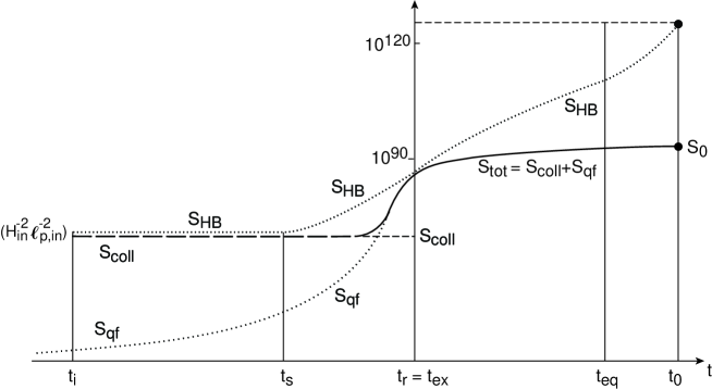
Figure 1: Entropy history from the onset of PBB inflation till today. Various contributions to the entropy budget of our Universe are shown together with the Hubble entropy bound $S_{HB}$. See text for explanation.

It is helpful to follow the evolution of various contributions to (and bounds on) entropy with the help of Fig. 1. At time $t=t_{i}$, corresponding to the first appearance of a horizon, we can use the Bekenstein–Hawking formula to argue that

$$S_{coll}\sim(R_{in}/l_{P,in})^{2}\sim(H_{in}l_{P,in})^{-2}=S_{HB}\;,$$ (10)

where we have used the fact [20] that the initial size of the black-hole horizon determines also the initial value of the Hubble parameter. Thus, at the onset of collapse/inflation, entropy, without any fine-tuning, is as large as allowed by the HEB. As a confirmation of this, note that $S_{coll}$ is also on the order of the number of quanta needed for collapse to occur [20]. We have implicitly assumed the initial state of the system to be at small string coupling: consequently, quantum fluctuations are very small, and contribute, initially, a negligible amount $S_{qf}$ to the total entropy.

After a short transient phase, dilaton-driven inflation (DDI) should follow [19, 20] and last until $t_{s}$, the time at which a string-scale curvature is reached. We expect this classical process not to generate further entropy (unless more energy flows into the black hole, but this would only increase its total comoving volume), but what happens to the HEB? Well, it stays constant, thus keeping the bound saturated, as the result of a well known “conservation law” of string cosmology [23], which reads $(l^{2}_{P}=e^{\phi}l^{2}_{s})$

$$\partial_{t}\left(e^{-\phi}\sqrt{g}H\right)=\partial_{t}\left((\sqrt{g}H^{3})~{}~{}(e^{-\phi}H^{-2})\right)=\partial_{t}\left(n_{H}S_{H}\right)=0~{}.$$ (11)

Comparing this with (8), we recognize that (11) simply expresses the time independence of the HEB during the DDI phase. At the beginning of the DDI phase $n_{H}=1$, and the whole entropy is in a single Hubble volume; however, as DDI proceeds, the same total amount of entropy becomes equally shared between very many Hubble volumes until, eventually, each one of them contributes a small number. Also, if we assume that the string coupling is still small at the end of DDI, we can easily argue that the entropy in quantum fluctuations remains at a negligible level during that phase.

Is this going to continue indefinitely? Hopefully not: we want to exit from the DDI phase and enter, eventually, some kind of FRW cosmology! This is the well-known exit problem of string cosmology [24]. Two diagrams can be helpful when discussing this problem. In Fig. 2 we plot, on a linear scale, the Hubble parameter against a (duality-invariant) combination of the rate of growth of the dilaton and $H$. DDI lies in the first quadrant of this plane, FRW in the second. If exit occurs, the two branches should smoothly connect (dotted line). In Fig. 3, we show instead, on a log-log plot, $H$ as a function of the string coupling. DDI solutions now correspond to the parallel straight lines going upwards to the right. Different straight lines correspond to different initial conditions (different classical moduli). The horizontal boundary corresponds to the reach of string-scale curvatures, where $\alpha^{\prime}$ corrections should become essential in order to prevent the singularity.

Let us assume for the moment initial conditions such that we hit this boundary while the coupling is still small and ask whether the HEB may come to our help. In fact, since the HEB is saturated all the time during DDI, it cannot decrease after this phase ends. This condition reads:

$$\partial_{t}(e^{-\phi}\sqrt{g}H)\geq 0\Rightarrow(\dot{\phi}-3H)\leq\dot{H}/H\;.$$ (12)

This constraint is very welcome. As $\alpha^{\prime}$ corrections intervene to stop the growth of $H$, the HEB forces $\dot{\phi}-3H$ to decrease and even to change sign if $H$ stops growing. But this is just what is needed to make the DDI branch flow into the FRW branch in Fig. 2!

Consider now the second possibility [25], the case in which strong coupling is reached first, i.e. while the curvature is still small in string units. In this case we can neglect $\alpha^{\prime}$ corrections but not loop corrections, particle production, and back-reaction effects. When will exit occur? It has been assumed [26] that it does when the energy in the quantum fluctuations (which can be easily estimated [23]) becomes critical, i.e. when

$$\rho_{qf}\sim N_{eff}~{}H^{4}_{max}=\rho_{cr}=e^{-\phi_{exit}}M_{s}^{2}~{}H^{2}_{max}~{},$$ (13)

where $N_{eff}$ is the effective number of particle species produced. This gives the exit condition $N_{eff}~{}e^{\phi_{exit}}~{}l_{s}^{2}~{}H^{2}_{max}=1$, i.e. the rightmost boundary in Fig. 3. Let us show that this is also the boundary where the HEB is saturated. Using known results on entropy production due to the cosmological squeezing of vacuum fluctuations [27], and the previous constraint, we find:

$$S_{qf}^{({\rm ex})}\sim N_{eff}~{}H^{3}_{max}V\sim e^{-\phi_{exit}}l_{s}^{-2}~{}H_{max}V\sim l_{P}^{-2}~{}H_{max}V\sim S_{HB}^{({\rm ex})}~{}.$$ (14)

Note that the existence of this boundary can also be argued for [25] on the basis of $M$-theory: Kaluza–Klein modes living in the 11th dimension become tachyonic when this critical line is reached.

In conclusion, the entropy and arrow-of-time problems are neatly solved, in PBB cosmology, by the identification of our observable Universe with the interior of a large, primordial black hole. The entropy of the black hole is large, because of its size ($>10^{20}l_{s}$) and, therefore, as with other features of PBB cosmology, this can be objected to as huge fine-tuning [28]. My answer to this objection, as to the others, is simple: the classical collapse/inflation process is scale-free; it should therefore lead to a flattish distribution of horizon sizes, extending from a minimal stringy size to very large “macroscopic” scales. Given such a size, no other ratio is tuned to a particularly large or small value. Next, there is a built-in mechanism to provide saturation of the HEB till the end of the DDI phase, and for the HEB to force an exit to the radiation-dominated FRW phase. From there on, the entropy budget story is simple: our entropy remains, to date, roughly constant and around $10^{90}$, while $S_{BH}$ keeps increasing –at somewhat different rates– during the radiation- and matter-dominated epochs, reaching about $10^{120}$ today. Thus our entropy has still a long way to go while it keeps fixing our arrow-of-time!

It is a pleasure to thank the organizers of this meeting for their kind invitation and to wish François many more years of highly rewarding research.

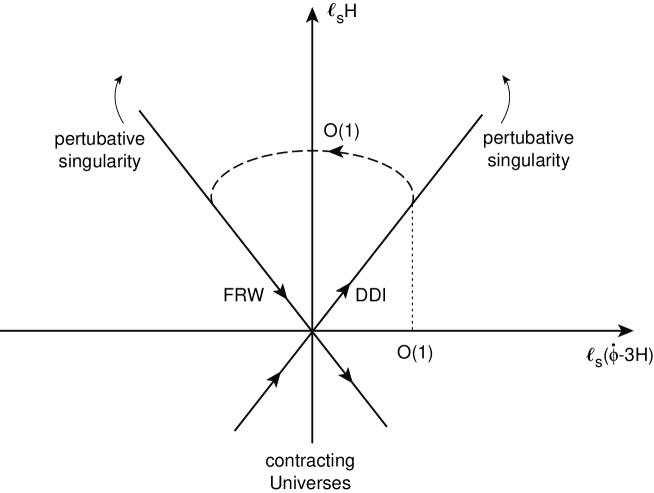
Figure 2: The standard phase diagram of string cosmology showing the duality-related inflationary and FRW branches and a possible (dashed) path connecting the two

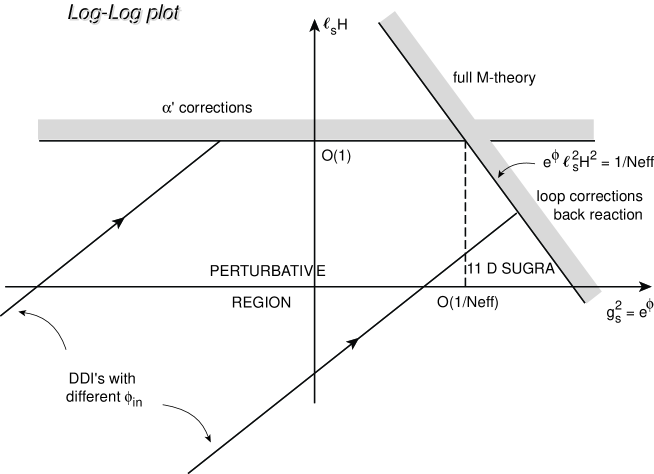
Figure 3: Another phase diagram showing different perturbative solutions as they hit boundaries where either curvature or coupling become large, depending on initial data

References

- [1]
- [2] R. Penrose, The Emperor’s new mind (Oxford University Press, New York, 1989), Chapter 7.
- [3] J. D. Bekenstein, Phys. Rev. D23 (1981) 287; D49 (1994) 1912, and references therein.
-
[4]
G. ’t Hooft, Abdus Salam Festschrift: a collection of talks, eds.
A. Ali, J. Ellis and S. Randjbar-Daemi (World Scientific, Singapore, 1993), gr-qc/9321026;
L. Susskind, J. Math. Phys. 36 (1995) 6377, and references therein. - [5] G. Veneziano, in Hot Hadronic Matter: Theory and Experiments, Divonne, June 1994, eds. J. Letessier, H. Gutbrod and J. Rafelsky, NATO-ASI Series B: Physics, 346 (Plenum Press, New York 1995), p. 63.
- [6] G. Veneziano, Europhys. Lett. 2 (1986) 133.
- [7] J. D. Bekenstein, Int. J. Theor. Phys. 28 (1989) 967.
- [8] W. Fischler and L. Susskind, Holography and cosmology, hep-th/9806039.
- [9] S. K. Rama and T. Sarkar, Phys. Lett. B450 (1999) 55, hep-th/9812043.
- [10] N. Kaloper and A. Linde, Cosmology vs. Holography, hep-th/9904120.
- [11] E. W. Kolb and M. S. Turner, The early Universe (Addison-Wesley, Redwood City, CA, 1990); A.D. Linde, Particle physics and inflationary cosmology (Harwood, New York, 1990).
- [12] D. Bak and S.-J. Rey, Holographic principle and string cosmology, hep-th/9811008.
- [13] A. K. Biswas, J. Maharana and R.K. Pradhan, The holography principle and pre-big bang cosmology, hep-th/9811051.
- [14] R. Bousso, A Covariant Entropy Conjecture, hep-th/9905177; Holography in General Space-Times, hep-th/9906022.
- [15] B. J. Carr and S. W. Hawking, Mon. Not. Roy. Astr. Soc. 168 (1974) 399; B. J. Carr, Astrophys. J. 201 (1975) 1; I. D. Novikov and A. G. Polnarev, Astron. Zh. 57 (1980) 250 [Sov. Astron. 24 (1980) 147].
- [16] G. Veneziano, Pre-bangian origin of our entropy and time arrow, hep-th/9902126.
- [17] R. Easther and D. A. Lowe, Holography, Cosmology, and the Second Law of Thermodynamics, hep-th/9902088; D. Bak and S.-J. Rey, Cosmic Holography, hep-th/9902173.
- [18] R. Brustein, The Generalized Second Law of Thermodynamics in Cosmology, gr-qc/9904061.
- [19] G. Veneziano, Phys. Lett. B406 (1997) 297; A. Buonanno, K.A. Meissner, C. Ungarelli and G. Veneziano, Phys. Rev. D57 (1998) 2543.
- [20] A. Buonanno, T. Damour and G. Veneziano, Nucl. Phys. B543 (1999) 275, hep-th/9806230.
- [21] G. Veneziano, Inflating, warming up, and probing the pre-bangian Universe, hep-th/9902097.
- [22] S. W. Hawking and R. Penrose, Proc. Roy. Soc. Lond. A314 (1970) 529.
- [23] G. Veneziano, Phys. Lett. B265 (1991) 287; M. Gasperini and G. Veneziano, Astropart. Phys. 1 (1993) 317. An updated collection of papers on the pre-big bang scenario is available at http://www.to.infn.it/~gasperin/.
- [24] R. Brustein and G. Veneziano, Phys. Lett. B329 (1994) 429; N. Kaloper, R. Madden and K.A. Olive, Nucl. Phys. B452 (1995) 677, Phys. Lett. B371 (1996) 34; R. Easther, K. Maeda and D. Wands, Phys. Rev. D53 (1996) 4247; M. Gasperini, M. Maggiore and G. Veneziano, Nucl. Phys. B494 (1997) 315; R. Brustein and R. Madden, Phys. Lett. B410 (1997) 110, Phys. Rev. D57 (1998) 712.
- [25] M. Maggiore and A. Riotto, D-branes and cosmology, hep-th/9811089.
- [26] G. Veneziano, in Effective theories and fundamental interactions, Erice, 1996, ed. A. Zichichi (World Scientific, Singapore, 1997), p. 300; A. Buonanno, K. A. Meissner, C. Ungarelli and G. Veneziano, JHEP01, 004 (1998).
- [27] M. Gasperini and M. Giovannini, Phys. Lett. B301 (1993) 334, Class. Quant. Grav. 10 (1993) L133; R. Brandenberger, V. Mukhanov and T. Prokopec, Phys. Rev. Lett. 69 (1992) 3606, Phys. Rev. D48 (1993) 2443.
- [28] M. Turner and E. Weinberg, Phys. Rev. D56 (1997) 4604; N. Kaloper, A. Linde and R. Bousso, Phys. Rev. D59 (1999) 043508.