Abstract

We show that in certain limits the (1+1)-dimensional massive Thirring model at finite temperature $T$ is equivalent to a one-dimensional Coulomb gas of charged particles at the same $T$. This equivalence is then used to explore the phase structure of the massive Thirring model. For strong coupling and $T$ $\gg m$ (the fermion mass), the system is shown to behave as a free gas of “molecules” (charge pairs in the Coulomb gas terminology) made of pairs of chiral condensates. This binding of chiral condensates is responsible for the restoration of chiral symmetry as $T\rightarrow\infty$. In addition, when a fermion chemical potential $\mu\neq 0$ is included, the analogy with a Coulomb gas still holds with $\mu$ playing the rôle of a purely imaginary external electric field. For small $T$ and $\mu$ we find a typical massive Fermi gas behaviour for the fermion density, whereas for large $\mu$ it shows chiral restoration by means of a vanishing effective fermion mass. Some similarities with the chiral properties of low-energy QCD at finite $T$ and baryon chemical potential are discussed.

1 Introduction

The massive Thirring (MT) model in two space-time dimensions has been widely studied as a toy counterpart to low-energy QCD, since it does not include many of the complications arising in 3+1 dimensions. Amongst the features shared by the MT model and QCD is hadronisation (bosonisation). In this primitive version, the MT model is equivalent to the sine-Gordon (SG) model, both at zero and non-zero temperatures [1, 2, 3]. Viewed as a non-linear sigma model (NLSM) in 1+1 dimension for a single Goldstone boson with an explicit symmetry breaking term, the SG model mimics the chiral Lagrangian for low-energy, strongly coupled QCD (whose rôle is played here by the MT model) where the lowest energy excitations of the vacuum are the Goldstone bosons. In addition, the solitonic excitations of the SG model (kinks, for brevity) correspond to Thirring fundamental fermions and hence they are the analogue of QCD baryons or, alternatively, the NLSM skyrmions [4].

This paper is the second in a series concerning the statistical mechanical features of those models. In [3], the MT/SG system and their equivalences (bosonisation) were analysed at finite temperature $T>0$ and non-zero fermion number chemical potential $\mu\neq 0$. It was shown that when there is a non-zero net fermion number in the MT model, a topological term arises in the dual SG model which counts the number of kinks minus antikinks [3]. Physically this term represents the thermal bosonisation of fermions into kinks and it reflects the existence of pure fermion excitations in the thermal bath. The same term appears in the exactly solvable massless Thirring model [5], and a similar contribution for a nonzero baryon chemical potential in the low-energy QCD chiral Lagrangian was obtained in [6]. However, the massless Thirring model, dual to the Schwinger model, has a much less rich and relevant structure if we have QCD in mind, and we shall not consider it here, except as a limiting case.

The purpose of the present paper is to analyse the thermodynamics of the MT model, calculating physical quantities such as the pressure, the fermion condensate (the order parameter of the chiral symmetry) and the fermion number density. We believe this to be important for obtaining a better understanding of crucial physical phenomena such as the QCD chiral phase transition, not only at finite temperature but also at finite baryon density [7].

We now introduce the model. In Euclidean space-time with metric $(+,+)$ the Lagrangian density of the MT model is

$${\cal{L}}_{MT}[\bar{\psi},\psi]=-\bar{\psi}(\not{\!{\partial}}+m_{0})\psi+\frac{1}{2}g^{2}j_{\mu}(x)j^{\mu}(x).$$

Here $\psi$ is a two-component fermionic field, the $0$ subscript denotes bare quantities and $j_{\mu}(x)=\bar{\psi}(x)\gamma_{\mu}\psi(x)$ where the Euclidean $\gamma$ matrices may be found in [3]. For $g^{2}>0$ forces are attractive and the theory is super-renormalisable. For $-1/2<g^{2}/\pi\leq 0$, further renormalisations need to be carried out as discussed in reference [8] for example, whereas for $g^{2}/\pi\leq-1/2$ the theory is no longer renormalisable [9]. Throughout this paper we take $g^{2}>0$ unless otherwise stated. With QCD in mind we are interested in strong coupling. In this we are aided by the general result that the natural parameter in which to express results is $(1+g^{2}/\pi)^{-1}$. This is understood by the explicit nature of the duality with the SG model, with Lagrangian density

$${\cal L}_{SG}[\phi]=\frac{1}{2}\partial_{\mu}\phi\partial^{\mu}\phi-\frac{\alpha_{0}}{\lambda^{2}}\cos\lambda\phi$$

where $\phi$ is a real scalar field. Recall that these models are equivalent only in the weak sense, i.e. for vacuum expectation values and thermal averages, provided that their renormalised constants are related through [1]

$$\frac{\lambda^{2}}{4\pi} = \frac{1}{1+g^{2}/\pi},$$ (1.1)

$$\frac{\alpha}{\lambda^{2}} = \rho\,m,$$ (1.2)

where $\rho$ is the renormalisation scale and $m$ the renormalised mass at that scale. Thus large positive $g^{2}$ corresponds to small $\lambda^{2}$, for which approximations can be well controlled.

With QCD in mind, we will be interested in the chiral properties of the MT model as well as of physical quantities such as the pressure. The chiral $U(1)$ transformations are $\psi\rightarrow\exp(ia\gamma^{5})\psi$ for the fermions and $\phi\rightarrow\phi+a/\lambda$ for the bosons with $a$ real arbitrary. The massless Thirring model is chiral invariant but the fermion mass term breaks that symmetry explicitly. Similarly the free boson theory is chiral invariant, whereas the $\cos\lambda\phi$ term in the SG model breaks it. Both models have still a residual ZZ invariance, corresponding to the choice $a=2\pi n$ with $n$ any integer. It is important to remark that in two space-time dimensions, the breaking of a continuous symmetry ($U(1)\rightarrow\mathchoice{\hbox{\cmss Z\kern-4.79993ptZ}}{\hbox{\cmss Z\kern-4.79993ptZ}}{\lower 0.9pt\hbox{\cmsss Z\kern-2.79996ptZ}}{\lower 1.2pt\hbox{\cmsss Z\kern-2.79996ptZ}}$ in this case) cannot be spontaneous [10]. The $U(1)$ and ZZ symmetries are, respectively, the counterparts of the chiral and isospin symmetries for QCD, $\alpha_{0}$ and $\lambda$ playing the rôle of the pion mass squared and the inverse of the pion decay constant respectively in the effective chiral Lagrangian to lowest order, i.e. the NLSM [11]. These generalities apart, the identification (1.1) which, for strong coupling becomes $\lambda g\approx 2\pi$, is the only attribute of the SG theory that we shall use. Depending on which is most convenient, we shall switch between the use of $g$ and $\lambda$. This is not to say that the SG model has no interest in its own right. It fact, it is an ideal testbed for summation schemes for the pressure and, as such, will be considered elsewhere [12]. It is also of direct relevance to the study of kinks in Josephson junctions [13].

In order to make progress we comment on a further property of the 2D MT model that also has a counterpart in QCD: at $T=0$ and $\mu=0$ it is also equivalent to a 2D classical statistical-mechanical system which consists of non-relativistic particles of charge $\pm q$ (a Coulomb gas) at a temperature $T_{CG}$ [8, 14]. Before clarifying the form of this analogy, we comment that one of the aims of this paper is to understand whether a similar equivalence holds when the MT model is heated to a non-zero temperature $T$ and for $\mu\neq 0$. If it does, we will then be able to use the simpler Coulomb gas system to explore its phase space. It has not yet proved possible to perform similar calculations for QCD, as represented in [15], in which the Coulomb gas is composed of monopoles.

Indeed, one of our conclusions is that at high temperature $T$, the MT model can be equivalent to a one dimensional Coulomb gas of particles at the same temperature $T$. This is not the case for the $T=0$ MT model, for which

$$T_{CG}=\frac{2\pi q^{2}}{\lambda^{2}}$$

leading to a Kosterlitz-Thouless (metal-insulator) transition at $\lambda^{2}=8\pi$ [14]. The 1D Coulomb gas model has been solved exactly [16, 17] and we use those results to extract information on the behaviour of observables such as the pressure and chiral condensate of the MT model. Furthermore, when $\mu\neq 0$ in the MT model, we show that the analogy with a 1D Coulomb gas still holds with $\mu$ playing the rôle of a purely imaginary external electric field.

This paper is organised as follows. In section 2 we analyse the conditions under which the equivalence which a 1D Coulomb gas holds. Having specified this “dimensionally reduced” regime, the exact link between the parameters of the different models is then specified in section 3 where the pressure of the MT model is also calculated. Section 4 is concerned with the fermion condensate. We see that for large $g$ and $T$ $\gg m$, the MT model behaves as a free gas of “molecules” made of pairs of chiral condensates. This binding of chiral condensates is responsible for the restoration of chiral symmetry as $T\rightarrow\infty$, and no phase transition takes place. The effects of a fermion chemical potential $\mu\neq 0$ on the pressure and fermion density are discussed in section 5.

2 Dimensional reduction of the $T>0$ MT model.

At nonzero temperature $T$ and zero chemical potential $\mu=0$ the MT model partition function is given by [2, 3]

$$Z_{MT}(T)=Z_{0}^{F}(T)\sum_{n=0}^{\infty}\left(\frac{1}{n!}\right)^{2}\left[\frac{\rho\,m}{2}\left(\frac{T}{\rho}\right)^{\lambda^{2}/4\pi}\right]^{2n}F_{2n}(\lambda,T,L).$$ (2.1)

Here $Z_{0}^{F}(T)$ is the partition function for a two-dimensional free massless Fermi gas, which, ignoring irrelevant vacuum terms, is given by

$$Z_{0}^{F}(T)=\exp\left[\frac{\pi LT}{6}\right],$$

and the function $F_{2n}(\lambda,T,L)$ is

$$F_{2n}(\lambda,T,L)=\prod_{j=1}^{2n}\int_{0}^{\beta}d\tau_{j}\int_{0}^{L}dq_{j}\prod_{k<j}\left[Q^{2}(x_{j}-x_{k})\right]^{\epsilon_{j}\epsilon_{k}\lambda^{2}/4\pi}.$$ (2.2)

Here $x_{j}\equiv(\tau_{j},q_{j})$, $\beta=T^{-1}$,

$$\epsilon_{j}=\left\{\begin{array}[]{cl}+&j=1,\dots,n\\ -&j=n+1,\dots,2n\end{array}\right.$$

and $L$ is the length of the system. We will eventually take the thermodynamic or $L\rightarrow\infty$ limit in all our results. It must be clarified though that the $L\rightarrow\infty$ limit will be taken always keeping $\beta$ finite. In fact, we will see explicit examples below in which the $L\rightarrow\infty$ and $T\rightarrow 0^{+}$ limit do not commute. Finally, the $Q$ variable in (2.2) also appears in the finite temperature free massless boson and fermion propagators [2] and is given by

$$Q^{2}(q,\tau)=\sinh(\frac{\pi(q+i\tau)}{\beta})\sinh(\frac{\pi(q-i\tau)}{\beta})$$ (2.3)

betraying its conformal origins. As discussed in [3], the integrals in (2.1) are convergent for $g^{2}>0$.

Equation (2.1) will be our starting point here. First, notice that

$$Q^{2}(q,\tau)\longrightarrow\frac{1}{4}\exp{\frac{2\pi|q|}{\beta}}\qquad\mbox{for}\quad\frac{\pi|q|}{\beta}\gg 1\qquad\forall\tau.$$ (2.4)

The key observation is therefore that if we were allowed to replace the $Q^{2}$ functions in (2.1) by their asymptotic values (2.4) then, with appropriate definitions, (2.1) would resemble the grand canonical partition function of a one-dimensional classical gas of charged particles with positions labelled by $q_{i}$. Remember that the two-particle Coulomb potential for charges $\pm\sigma$ at points $q_{1}$ and $q_{2}$ on the line is $V\propto\pm\sigma^{2}|q_{1}-q_{2}|$. This 1D Coulomb gas system was studied a long time ago [16, 17] and it can be solved exactly. We shall explore this analogy later on in section 3 and use the exact results to calculate the pressure and chiral condensate of the MT model.

Before doing so, however, we need to establish the conditions under which the replacement given in (2.4)—which we will denote dimensional reduction (DR)—can be safely made. This DR regime is the 2D analogue of more complicated situations analysed in the thermal field theory literature, which roughly works for high temperatures and large distances [18, 19, 20].

Clearly the regions in the integrand (2.1) where the replacement (2.4) is not allowed are those where $|q_{j}-q_{k}|\leq\beta/\pi$. In those regions the dominant contributions to the integral come from $x_{j}\simeq x_{k}$ with $\epsilon_{j}\epsilon_{k}=-1$ since

$$Q^{2}(q,\tau)\longrightarrow(\pi T)^{2}(q^{2}+\tau^{2})\qquad\mbox{for}\quad(q,\tau)\rightarrow(0^{+},0^{+}).$$

Thus, on the one hand, we expect that for high enough $T$ the contribution (arising in the denominator) can be neglected. On the other hand, the above contributions become more important as $g^{2}$ decreases, so that one may also think that for large enough $g^{2}$ the approach could be equally justified. Bearing these considerations in mind, we shall analyse the limits of high $T$ and large $g^{2}$ separately in sections 2.1 and 2.2.

Before proceeding, two comments are in order regarding the expression (2.1). First, every term in the $n$-sum picks up an overall $\beta L$ factor. In other words, the number of two-dimensional independent variables in the integral is actually $2n-1$. This is most easily seen by changing variables to

$$z_{1}=x_{1}-x_{2},z_{2}=x_{2}-x_{3},\dots,z_{2n-1}=x_{2n-1}-x_{2n},z_{2n}=x_{2n}$$ (2.5)

so that in (2.1)

$$x_{j}-x_{k}=\sum_{i=j}^{k-1}z_{i}$$

and therefore the integrand is independent of $z_{2n}$, which yields the $\beta L$ factor. Notice that this is typical of closed loops in perturbation theory [21]. Order by order one has to consider all possible connected closed diagrams for the partition function and the $\beta L$ factor is just the consequence of total energy-momentum conservation. One should bear in mind that the physically relevant object is not the partition function but the pressure, defined in the thermodynamic limit as

$$P=\lim_{L\rightarrow\infty}\frac{1}{\beta L}\log Z_{MT}(L,T)$$ (2.6)

which behaves as an intensive quantity.

The second comment concerns the scale dependence. The partition function (2.1) is scale independent (and so is the pressure) since the explicit dependence on the renormalisation scale $\rho$ is exactly cancelled by the implicit dependence of the mass $m(\rho)$ (see [3] for details). Thus, unless otherwise stated and whenever dealing with scale-independent objects in the following, we will choose for convenience $\rho=m$, the renormalised mass of the Thirring fermion.

2.1 High $T$ limit

Let us rescale $q_{j}\rightarrow q_{j}\beta$ and $\tau_{j}\rightarrow\tau_{j}\beta$ $\forall j$ in (2.2). Then all the relevant $T$ dependence is now outside the integrals in (2.2) since in the thermodynamic limit $\eta=L/\beta\rightarrow\infty$ the integrals are finite as long as $\lambda^{2}<4\pi$—excluding of course the $\eta$ overall factor mentioned above. Then, choosing $\rho=m$, the series in (2.1) yields effectively a perturbative series in $(m^{2}/T^{2})^{(\pi+2g^{2})/(2\pi+2g^{2})}$ = $(m^{2}/T^{2})^{1-\lambda^{2}/8\pi}$:

$$Z_{MT}(T)=Z_{0}^{F}(T)\left\{1+\sum_{n=1}^{\infty}\left(\frac{1}{n!}\right)^{2}\left[2\left(\frac{m^{2}}{T^{2}}\right)^{1-\lambda^{2}/8\pi}\right]^{2n}\frac{1}{4}\eta f_{2n}(\lambda)\right\}$$

with $f_{2n}(\lambda)$ independent of $\eta$ in the thermodynamic limit and given by

$$f_{2n}(\lambda)=\prod_{j=1}^{2n-1}\int_{0}^{1}dz_{j}^{0}\int_{0}^{\infty}dz_{j}^{1}\prod_{k<j+1}\left[Q^{2}(\beta\sum_{i=k}^{j}z_{i})\right]^{\epsilon_{j+1}\epsilon_{k}\lambda^{2}/4\pi},$$

where $z_{j}\equiv(z_{j}^{0},z_{j}^{1})$ is defined in (2.5). It follows from (2.3) that $Q^{2}(\beta q,\beta\tau)$ is independent of $\beta$. Therefore, to leading order in $m/T$, we can write the MT pressure as

$$P_{MT}(\lambda,T)=P_{MT}^{asym}(\lambda,T)\left[1+\frac{6}{\pi}\left(\frac{m}{T}\right)^{4-\lambda^{2}/2\pi}\!\!\!\!\!\!\Delta f_{2}(\lambda)\right]+{\cal O}\left(\frac{m}{T}\right)^{8-\lambda^{2}/\pi}$$ (2.7)

where the $asym$ superscript denotes the value obtained by replacing the $Q$’s by their asymptotic values in (2.4), and $\Delta f_{2}(\lambda)=f_{2}(\lambda)-f_{2}^{asym}(\lambda)$ with

$$f_{2}(\lambda)=\int_{0}^{\infty}dq\int_{0}^{1}d\tau\left[Q^{2}(\beta q,\beta\tau)\right]^{-\lambda^{2}/4\pi}$$ (2.8)

and

$$f_{2}^{asym}(\lambda)=\frac{2^{\lambda^{2}/2\pi+1}}{\lambda^{2}}.$$

We have evaluated numerically $\Delta f_{2}(\lambda)$ and the result is plotted in Figure 1. We see that it remains of ${\cal O}(1)$ until very close to the limiting case $\lambda^{2}/4\pi\raise 1.29167pt\hbox{$<$\kern-7.5pt\lower 4.30554pt\hbox{$\sim$}}1$, or $g^{2}\raise 1.29167pt\hbox{$>$\kern-7.5pt\lower 4.30554pt\hbox{$\sim$}}0$, where it diverges. Thus, the relative error for $T\gg m$ is at least of order $(m/T)^{2}$ and we can therefore conclude that for $T\gg m$, DR is valid for $g^{2}>0$.

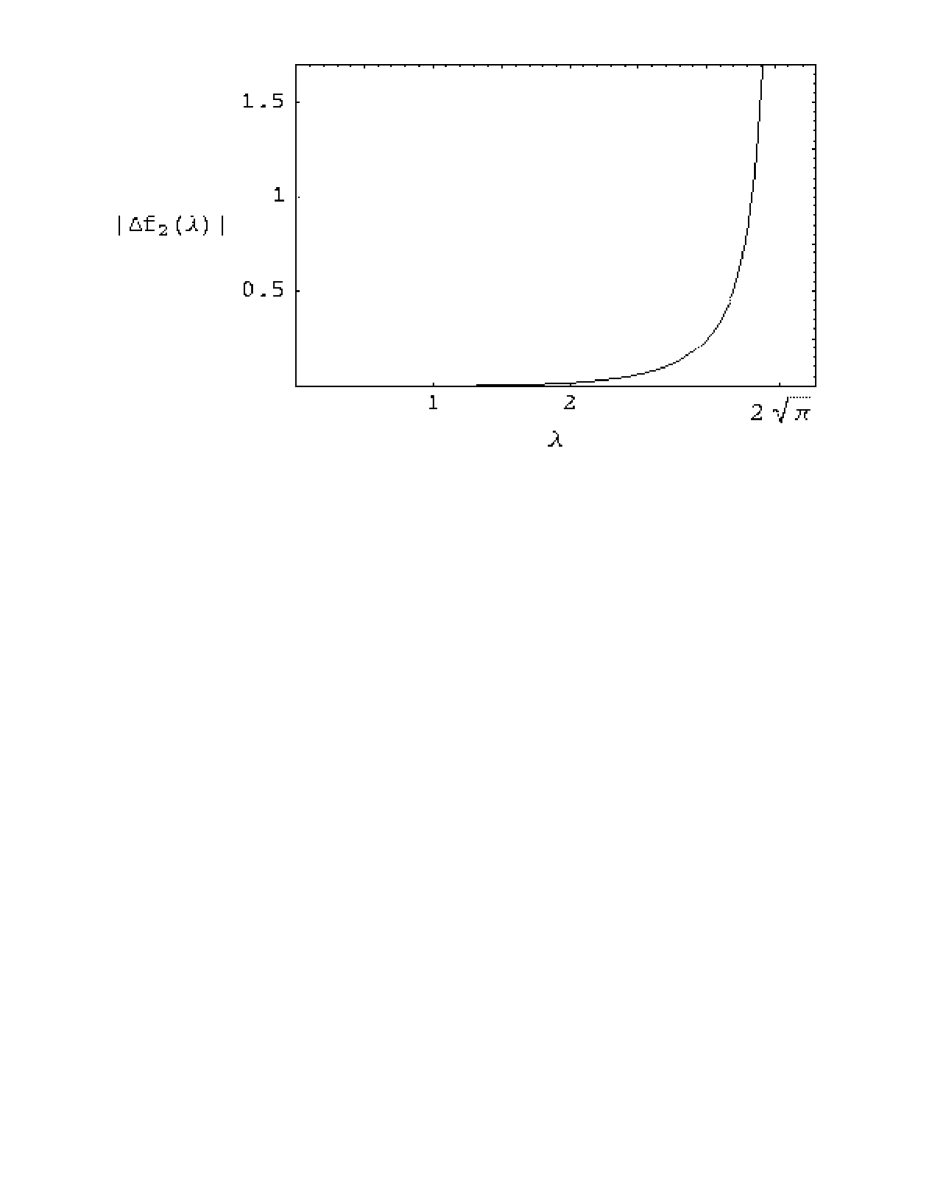
Figure 1: The function $\Delta f_{2}(\lambda)$

2.2 Strong coupling (large $g^{2}$) limit.

We would now like to study the pressure for $g^{2}/\pi\gg 1$ ($\lambda^{2}/4\pi\ll 1$). The first observation is that the integrals in (2.2) diverge if we set $\lambda=0$ and then take the limit $L\rightarrow\infty$. Therefore we shall keep $L$ finite and then take it to infinity (keeping $\beta$ finite) only when the pressure (2.6) is calculated. Then, expanding (2.2) in $\lambda^{2}/4\pi$ one obtains

$$F_{2n}(\lambda,T,L)=(\beta L)^{2n}\left\{1-\frac{n\beta\lambda^{2}}{\pi L}\int_{0}^{\eta}dq\int_{0}^{1}d\tau\log\left[Q^{2}(\beta q,\beta\tau)\right]+{\cal O}\left(\frac{\lambda^{2}}{4\pi}\right)^{2}\right\}.$$

Thus

$$F_{2n}(\lambda,T,L)=F_{2n}^{asym}(\lambda,T,L)-n(\beta L)^{2n}\frac{\lambda^{2}}{4\pi}\hat{I}(\eta)+{\cal O}\left(\frac{\lambda^{2}}{4\pi}\right)^{2}$$

with

$$\hat{I}(\eta)=\frac{4}{\eta}\left[\int_{0}^{\eta}dq\int_{0}^{1}d\tau\log\left[Q^{2}(\beta q,\beta\tau)\right]+2\eta\log 2-\pi\eta^{2}\right]$$ (2.9)

so that

$$Z_{MT}(T,\lambda,L) = Z_{MT}^{asym}(T,\lambda,L)-\frac{\lambda^{2}}{4\pi}\hat{I}(\eta)Z_{0}^{F}(T)\sum_{n=0}^{\infty}n\left(\frac{1}{n!}\right)^{2}\left[\frac{m^{2}}{2}\beta L\right]^{2n}+{\cal O}\left(\frac{\lambda^{2}}{4\pi}\right)^{2}$$

$$= Z_{MT}^{asym}(T,\lambda,L)-\frac{\lambda^{2}}{4\pi}\hat{I}(\eta)Z_{0}^{F}(T)\frac{z}{2}I_{0}^{\prime}(z)+{\cal O}\left(\frac{\lambda^{2}}{4\pi}\right)^{2}$$

where

$$z=m^{2}\beta L\left(\frac{T}{m}\right)^{\lambda^{2}/4\pi}$$ (2.10)

and $I_{0}(z)$ is the modified Bessel function of zeroth order. On the other hand,

$$Z_{MT}(T,\lambda,L)=Z_{0}^{F}(T)\sum_{n=0}^{\infty}\left(\frac{1}{n!}\right)^{2}\left(\frac{z}{2}\right)^{2n}+{\cal O}\left(\frac{\lambda^{2}}{4\pi}\right)=Z_{0}^{F}(T)I_{0}(z)+{\cal O}\left(\frac{\lambda^{2}}{4\pi}\right)$$ (2.11)

and $Z_{MT}^{asym}(T,\lambda,L)$ has the same leading order in $\lambda^{2}/4\pi$ as above. Therefore, we can write for the pressure

$$P_{MT}(T,\lambda)=P_{MT}^{asym}(T,\lambda)-\lim_{L\rightarrow\infty}\frac{1}{\beta L}\left[\frac{\lambda^{2}}{8\pi}\hat{I}(\eta)z\frac{I_{0}^{\prime}(z)}{I_{0}(z)}\right]+{\cal O}\left(\frac{\lambda^{2}}{4\pi}\right)^{2}.$$

Now, for large $z$ [22],

$$I_{0}(z)=\frac{e^{z}}{\sqrt{2\pi z}}+{\cal O}\left(\frac{1}{z}\right)\qquad\mbox{for}\quad z\gg 1$$

so that taking $L\rightarrow\infty$ we finally get

$$P_{MT}(T,\lambda)=P_{MT}^{asym}(T,\lambda)-\frac{m^{2}\lambda^{2}}{8\pi}\hat{I}(\eta\rightarrow\infty)+{\cal O}\left(\frac{\lambda^{2}}{4\pi}\right)^{2}.$$ (2.12)

Numerical analysis of the function $\hat{I}(\eta)$ shows that it clearly vanishes as $\eta\rightarrow\infty$. Therefore we have $\Delta P_{MT}={\cal O}(\lambda^{4})$. Although it might seem that this result is valid for any $T$, one has to be extremely careful when approaching the limit $T\rightarrow 0^{+}$. In fact, we see that expanding (2.10) in $\lambda$ yields logarithmic factors $\log T/m$ hidden in the ${\cal O}(\lambda^{4})$ in (2.12), but which will show up at next-to-leading order. Therefore the above results should not be trusted for temperatures $T\ll m$. This is just a consequence of the non-uniformity of the $T\rightarrow 0^{+}$ limit or, in other words, that the $L\rightarrow\infty$ and $T\rightarrow 0^{+}$ do not commute in general. Hence we will consider that our approach is justified for large $g^{2}/\pi$ and $T\raise 1.29167pt\hbox{$>$\kern-7.5pt\lower 4.30554pt\hbox{$\sim$}}m$. Recall that the presence of the $\log T/m$ factors in the $\lambda$ expansion may be also troublesome for very large $T$, which gives a hint that the high $T$ limit may not be compatible with perturbation theory, as has been noticed in more complicated situations [23]. In our case though, we have a well defined high $T$ expansion, namely our expansion in $(m^{2}/T^{2})^{1-\lambda^{2}/8\pi}$ discussed in section 2.1, which we will indeed be able to resum in the DR regime.

To summarise, the results of this section are that the range of validity of the DR approach which we will be considering for the pressure is

$$T\gg m ,\quad g^{2}>0,$$

$$T\raise 1.29167pt\hbox{$>$\kern-7.5pt\lower 4.30554pt\hbox{$\sim$}}m ,\quad\frac{g^{2}}{\pi}\gg 1.$$ (2.13)

We now turn to the 1D Coulomb gas system and specify exactly the link between it and the MT model.

3 The MT partition function as a Coulomb gas

Consider the partition function for a one-dimensional neutral classical non-relativistic gas of charged particles. In particular, take $N$ positively charged particles and $N$ negative ones, where the magnitude of the charge will be denoted by $\sigma$. In one dimension, these charges interact via a Coulomb potential proportional to $\pm\sigma^{2}$ and to the distance between them on the line. This system can be also interpreted as uniformly charged plane sheets moving along the direction normal to their planes [16, 17]. Then, the partition function in the grand canonical ensemble at fixed temperature $\theta$, fugacity $z$ and length $L$ is [16, 17]

$$\Omega(z,\theta,\sigma,L)=\sum_{N=0}^{\infty}\frac{z^{2N}}{(N!)^{2}}\left(\prod_{i=1}^{2N}\int_{0}^{L}dq_{i}\right)\exp\left[2\pi\sigma^{2}\theta^{-1}\sum_{1\leq j<i\leq 2N}\epsilon_{i}\epsilon_{j}|q_{i}-q_{j}|\right]$$ (3.1)

where $\epsilon_{i}=1$ for $i\leq N$ and $\epsilon_{i}=-1$ for $i>N$. The fugacity is related to the chemical potential $\mu$ by $z=\sqrt{2\pi M\theta}\exp\theta^{-1}\mu$, where $M$ is the mass of the particles. However, we will keep $z$ instead of $\mu$ here, so as not to confuse this chemical potential with the fermion chemical potential we will introduce in section 5. In the thermodynamic limit the pressure and the mean particle density are given by

$$P(z,\theta,\sigma) = \lim_{L\rightarrow\infty}\frac{\theta}{L}\log\Omega(z,\theta,\sigma,L)$$

$$n(z,\theta,\sigma) = \frac{\ll 2N\gg}{L}=\theta^{-1}z\frac{\partial}{\partial z}P(z,\theta,\sigma)$$

where $\ll\cdot\gg$ denotes the statistical average in the above ensemble. We therefore realise that by making the replacement (2.4) in (2.1) and setting $\rho=m$, one can write

$$Z_{MT}(T,L)=Z_{0}^{F}(T,L)\Omega\left(z=\frac{m^{2}}{2T}\left(\frac{2T}{m}\right)^{\lambda^{2}/4\pi},\theta=T,\sigma=\frac{\lambda T}{\sqrt{4\pi}},L\right).$$ (3.2)

This is the central equivalence of this paper. Its utility lies in the fact that the above classical problem was solved analytically in references [16, 17]. There it was shown that for small $\theta$ the 1D Coulomb gas behaves as a gas of free “molecules”, made up of $+-$ charges pairs bound together (since the mean kinetic energy is much smaller than the mean potential energy). The main features of this phase are: i) The pressure is small compared to $2\pi\sigma^{2}$, which represents the pressure between $+-$ charges, and ii) The probability density of finding a $+-$ pair within a given distance $r$ is much bigger than that of finding a $++$ pair for distances $r$ less than a typical “molecule” size, which on the other hand is much smaller than the typical inter-particle distance. On the contrary, for large $\theta$ (when the mean kinetic energy is much larger than the mean potential energy) the charges are completely deconfined, forming an electrically neutral “plasma” of $2N$ free particles, where the pressure is higher than in the “molecule” phase. The crucial point in our case is that, from (3.2) we see that the unit charge grows with temperature ($\sigma\propto T$) and therefore the above phases are going to be reversed (high $T$ “molecule” phase and low $T$ “plasma” phase), as we shall now see in detail.

Let us first quote the result for the pressure in [17]

$$P(z,\theta,\sigma)=2\pi\sigma^{2}\gamma_{0}\left[\frac{z\theta}{2\pi\sigma^{2}}\right]$$

where $\gamma_{0}(\hat{z})$ is the highest eigenvalue of Mathieu’s differential equation

$$\left[\frac{d^{2}}{d\phi^{2}}+2\hat{z}\cos\phi\right]y(\phi)=\gamma y(\phi)$$ (3.3)

with $y(\phi+2\pi)=y(\phi)$. Notice that (3.3) differs slightly from the notation customarily used for Mathieu’s equation (see for instance [22]), which is recovered by setting $\gamma=-a/4$, $\hat{z}=-q/4$ and $\phi=2v$. Therefore, from (3.2) we obtain for the full pressure of the MT model in the DR regime:

$$P_{MT}(T)=\frac{\pi}{6}T^{2}+P_{C}(T,\lambda)$$ (3.4)

with the “Coulomb gas” pressure being given by

$$P_{C}(T,\lambda)=\frac{\lambda^{2}T^{2}}{2}\gamma_{0}\left[\frac{m^{2}}{\lambda^{2}T^{2}}\left(\frac{2T}{m}\right)^{\lambda^{2}/4\pi}\right].$$

Or, in terms of $g^{2}$,

$$P_{C}(T,g)=\frac{2\pi T^{2}}{1+g^{2}/\pi}\gamma_{0}\left[\frac{m^{2}}{4\pi T^{2}}\bigg{(}1+\frac{g^{2}}{\pi}\bigg{)}\left(\frac{2T}{m}\right)^{(1+g^{2}/\pi)^{-1}}\right].$$ (3.5)

The eigenvalues and eigenfunctions of the characteristic problem (3.3) are well known and tabulated. We refer to [22] for their general properties and quote here only those relevant for our purposes. For instance, the asymptotic limits of $\gamma_{0}(\hat{z})$ for very large and very small $\hat{z}$ are

$$\gamma_{0}(\hat{z}) \simeq 2\hat{z}^{2}+{\cal O}(\hat{z}^{4})\qquad\mbox{for}\quad\hat{z}\ll 1$$ (3.6)

$$\gamma_{0}(\hat{z}) \simeq 2\hat{z}-\sqrt{\hat{z}}+{\cal O}(1)\qquad\mbox{for}\quad\hat{z}\gg 1.$$ (3.7)

The relevant parameter setting the qualitative behaviour of the system is the argument of $\gamma_{0}$ in (3.5),

$$\hat{z}=\frac{m^{2}}{4\pi T^{2}}\bigg{(}1+\frac{g^{2}}{\pi}\bigg{)}\left(\frac{2T}{m}\right)^{(1+g^{2}/\pi)^{-1}}\;\;:$$ (3.8)

for small $\hat{z}$, the system is in the “molecule” phase, whereas for large $\hat{z}$ it is in the “plasma” phase. Let us then consider three separate limiting cases:

• $g^{2}\gg\pi$ and $T\gg mg/2\pi$: This is the very high $T$ regime and we have $\hat{z}\ll 1$, so that equations (3.6) and (3.5) give $P_{C}\sim m^{2}(m^{2}g^{2}/4\pi^{2}T^{2})$, i.e. the Coulomb pressure vanishes at high $T$ for large $g^{2}$. This is the “molecule” phase described in [16] in which the Coulomb charges tend to pair, thus lowering the pressure. As noted above, this “unexpected” behaviour of high temperature binding is just a consequence of the fact that our coupling “charge” $\sigma$ in (3.2) increases with $T$. Besides, when adding the free term in (3.4), the total pressure is an increasing function of $T$, behaving in the high $T$ (and large $g^{2}$) regime as a free gas of massless fermions. This is indeed the first indication that the “molecule” phase corresponds in fact to a phase of asymptotic chiral symmetry restoration. The reason is that we expect that if the chiral symmetry is restored, the system behaves roughly as the massless case which is chiral invariant. In other words, we would expect the effective fermion mass to vanish in the $T\rightarrow\infty$ limit when the system tends to restore the chiral symmetry.

• $g^{2}\gg\pi$ but $T\ll mg/2\pi$: Now equation (3.7) gives $P_{C}\sim m^{2}-\pi mT/g$. Since $\hat{z}\gg 1$, now we are in the “plasma” phase. Notice that this same result, to leading order, could have been obtained through our analysis for large $g$ in section 2.2, c.f. equation (2.11). Again we note that to ${\cal O}(\lambda^{2})$ in the expansion of $P_{C}$ there is a contribution proportional to $\lambda^{2}m^{2}\log(T/m)$ which prevents us from going to $T\ll m$. This is another reason why in the small $\lambda$ (large $g$) regime we can only trust DR for $T\raise 1.29167pt\hbox{$>$\kern-7.5pt\lower 4.30554pt\hbox{$\sim$}}m$, which is the region covered in this second case.

• $0<g^{2}\ll 1$ and $2\pi T\gg m$: we have now $\hat{z}\simeq m/2\pi T$. Again, $\hat{z}\ll 1$ and we are in the “molecular” phase. Remember that in this region we can only trust DR for $T\gg m$. Thus $P_{C}\sim m^{2}/\pi$ so that the pressure tends to a constant value for high $T$. Actually, if we were able to push our results formally to $g^{2}\leq 0$ $(\lambda^{2}\geq 4\pi)$, the pressure would start growing for large $T$. Clearly, our previous calculations in the MT model are not justified in this case, which at least would require extra renormalisations. However, from the viewpoint of the Coulomb gas only, there is no particular problem with taking $g^{2}$ negative. In other words, the dimensionally reduced theory is UV finite. Notice also that, as we make $g^{2}$ more negative, the Coulomb correction to the free boson gas term becomes more and more important. In particular, if we take $g^{2}/\pi\raise 1.29167pt\hbox{$<$\kern-7.5pt\lower 4.30554pt\hbox{$\sim$}}-1/2$ , $P_{C}$ would grow quadratically with $T$, thus being of the same order as the free contribution.

In Figure 2 we have plotted $P_{C}(T)$ in units of $m$ for different values of $g^{2}$. Notice that, as we have said before, we cannot claim that curve iv) corresponds to the MT model in the DR regime. We are simply extrapolating the Coulomb gas results to that point. As for curve iii), we should intend it as the limit of the dimensionally reduced MT model for very small but positive $g^{2}$, where we can still trust our DR approach, as long as we look only to the $T/m\gg 1$ tail of that curve. Note also that $P_{C}(T)$ is always a continuous function of the temperature and thus we do not see a phase transition in $T$, consistent with being in two dimensions. In Figure 3 we plot the Coulomb pressure and the total pressure for $g^{2}/\pi=1$ in order to estimate the size of the “Coulomb” gas correction to the free gas.

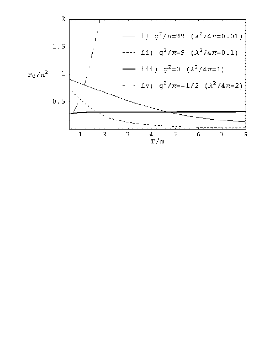
Figure 2: The Coulomb pressure $P_{C}(T,g)$.

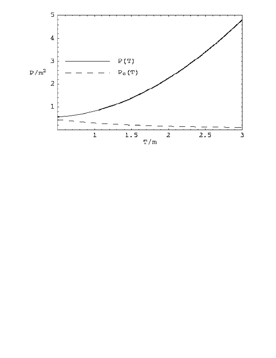
Figure 3: The total pressure and the Coulomb pressure for $g^{2}/\pi=1$

4 The chiral charges and “molecules”

In the previous section we have exploited the analogy of our dimensionally reduced MT partition function with that of a Coulomb gas on the line in order to calculate the pressure. In this section we will show that this analogy can be extended further, i.e. that it also works in the same way for other observables. In particular, we will concentrate on thermal averages of products of the operators

$$\sigma_{\pm}(x)=\frac{1}{2}\overline{\psi}(1\pm\gamma^{5})\psi$$

since these account for the chiral properties of the system. Under the chiral transformations discussed in the introduction, $\sigma_{\pm}(x)\rightarrow\exp(\pm 2ia)\sigma_{\pm}(x)$; in other words, the $\sigma_{\pm}$ operators have well defined $\pm$ chiral charge. Below we will show that in our Coulomb gas analogy they play the rôle of the charges, and the chiral invariant combination $\sigma_{+}\sigma_{-}$ will then represent a “molecule”. Thus by forming “molecules”, the system tends to restore the chiral symmetry, i.e. it behaves as the massless theory where only $\sigma_{+}\sigma_{-}$ combinations are allowed.

We will show below that the $\sigma_{\pm}$ correlators can be related with the 1D Coulomb gas reduced density functions discussed in [17]. These functions are defined as follows: $f_{\pm}(x)dx$ denotes the probability of finding a $\pm$ charge in the element $dx$; $f_{+-}(x_{1},x_{2})dx_{1}dx_{2}$ is the joint probability of finding a $+$ charge in $dx_{1}$ and a $-$ one in $dx_{2}$, and so on. It turns out that such density functions can also be exactly calculated [17]. We will only consider here the one-point and two-point functions, which will provide information on the relationship between Coulomb “molecule” pairing and the chiral symmetry, as explained above.

4.1 The fermion condensate and chiral symmetry vs “molecule” pairing

The first correlator we will analyse is just the one-point function, i.e. the condensate of $\sigma_{\pm}$. Observe that $\ll\sigma_{+}\gg\;=\;\ll\sigma_{-}\gg$ since the MT model is invariant under $\psi_{+}\leftrightarrow\psi_{-}$ where $\psi_{\pm}=(1/2)(1\pm\gamma^{5})\psi$ are the right and left-handed projections of the spinor field ($\phi\rightarrow-\phi$ in the SG model). This is a parity transformation and has nothing to do with the chiral transformations we have been discussing here. We shall implicitly make use of this $+\leftrightarrow-$ symmetry in the correlators throughout this section.

The scale invariant fermion condensate $m\ll\overline{\psi}\psi\gg$ is the order parameter of the chiral symmetry, exactly as the quark condensate in QCD. An immediate consequence of the absence of a phase transition in 2D is that the fermion condensate cannot vanish strictly at any temperature. On the other hand, for high temperatures $T\gg m$ we would expect that the mass scale $m$ becomes irrelevant and thus the system would restore the chiral symmetry, as indeed happens in the QCD chiral phase transition. This was already suggested by our previous analysis of the pressure. We may therefore expect the condensate to become smaller at large $T$ but never to reach zero. However, we do not expect chiral restoration for all positive values of $g^{2}$. An indication that this may actually be the case is the following. In the $g^{2}\rightarrow 0^{+}$ limit, the system should behave as a free massive fermion theory. However, it is not difficult to see that for $g=0$ the condensate behaves for $T\gg m$ as $\ll\bar{\psi}\psi\gg\simeq(m/\pi)\log(T^{2}/m^{2})$, so that there is clearly no chiral restoration in that case. Therefore we expect that chiral symmetry restoration is lost as the value of $g^{2}$ is decreased. Indeed, we have seen that behaviour already for the pressure, where the Coulomb correction to the massless term did not vanish for large $T$ and for very small $g^{2}$.

We will now show that in the DR regime the fermion condensate can be calculated exactly, thanks again to the analogy with the Coulomb gas. In fact we do not need to appeal to the density functions in this case since in the thermodynamic limit $L\rightarrow\infty$ the system is translationally invariant so that

$$m\ll\overline{\psi}\psi\gg\;=m\frac{\partial}{\partial m}P_{MT}(T).$$ (4.1)

Notice in particular that this implies that the regime in which we are allowed to replace the $Q$’s by their DR values for the condensate will be the same as for the pressure, i.e, (2.13).

Thus we only need to differentiate once in the expression obtained for the MT partition function in the DR regime to get the condensate. However, in order to clarify the procedure we will follow for the two point correlator and to understand better the analogy between Coulomb charges and chiral operators, let us relate the condensate with the one-charge density functions $f_{\pm}$ analysed in [17]. Those functions are given by $f_{+}=f_{-}$ with

$$f_{+}(z,\theta,\sigma,L;X) = \frac{1}{\Omega}\sum_{N=1}^{\infty}\frac{z^{2N}}{(N!)^{2}}\left(\prod_{i=1}^{2N}\int_{0}^{L}dq_{i}\right)\sum_{j=1}^{N}\delta(q_{j}-X)$$ (4.2)

$$\times \exp\left[2\pi\sigma^{2}\theta^{-1}\sum_{1\leq j<i\leq 2N}\epsilon_{i}\epsilon_{j}|q_{i}-q_{j}|\right]$$

$$= \frac{1}{\Omega}\sum_{N=1}^{\infty}\frac{z^{2N}}{N!(N-1)!}\left(\prod_{i=1}^{2N}\int_{0}^{L}dq_{i}\right)\delta(q_{N}-X)$$

$$\times \exp\left[2\pi\sigma^{2}\theta^{-1}\sum_{1\leq j<i\leq 2N}\epsilon_{i}\epsilon_{j}|q_{i}-q_{j}|\right],$$

where $\Omega$ is the partition function of (3.1). We see that in the $L\rightarrow\infty$ limit, a simple shift $q_{i}\rightarrow q_{i}+X$ $\forall i=1,\dots,2N$ ensures that $f_{+}$ is independent of $X$. In turn, notice that

$$f_{+}(z,\theta,\sigma,L)=\frac{1}{L}\int_{0}^{L}dXf_{+}(z,\theta,\sigma,L;X)=\frac{1}{2L}z\frac{\partial}{\partial z}\log\Omega(z,\theta,\sigma,L).$$ (4.3)

Now compare (4.2) with the expression obtained in [3] for the condensate:

$$m\ll\overline{\psi}\psi\gg = 2\frac{Z_{0}^{F}(T)}{Z_{MT}(T)}\sum_{n=0}^{\infty}\frac{1}{n!(n+1)!}\left[\frac{\rho\,m}{2}\left(\frac{T}{\rho}\right)^{\lambda^{2}/4\pi}\right]^{2(n+1)}$$

$$\times \prod_{j=1}^{n+1}\int_{0}^{\beta}d\tau_{j}\int_{0}^{L}dq_{j}\prod_{k<j}\left[Q^{2}(x_{j}-x_{k})\right]^{\epsilon_{j}\epsilon_{k}\lambda^{2}/4\pi}.$$

Thus, shifting $n\rightarrow n-1$ in the above equation, replacing the $Q$’s by their asymptotic values (2.4), fixing $\rho=m$ and comparing with $f_{+}$ we obtain in the DR regime

$$m\ll\overline{\psi}\psi\gg\;=2Tf_{+}\left(z=\frac{m^{2}}{2T}\left(\frac{2T}{m}\right)^{\lambda^{2}/4\pi},\theta=T,\sigma=\frac{\lambda T}{\sqrt{4\pi}},L\right).$$ (4.4)

Relation (4.4) is very interesting indeed since it supports the idea that the rôle of the Coulomb charges is played here by the $\sigma_{\pm}$ chiral correlators (in the DR regime). We will elaborate further on this issue below.

As it was said above, the fermion condensate can be obtained either using the analogy with the $f_{\pm}$ functions or by differentiating the pressure. We should then be able to rewrite (4.4) as (4.1), which would be a consistency check of our results. For that purpose, all we need to use is (4.3) and the equivalence between $\Omega$ and $Z_{MT}$ found in the previous section. In doing so it is important to leave the scale $\rho$ unfixed, since differentiating with respect to $m$ is a scale-dependent operation. After multiplying by $m$ the result becomes scale independent, and we can safely fix $\rho=m$. Once that consistency check has been performed, let us write the final expression for the fermion condensate as

$$m\ll\overline{\psi}\psi\gg=\frac{m^{2}}{2}\left(\frac{2T}{m}\right)^{(1+g^{2}/\pi)^{-1}}\gamma_{0}^{\prime}\left[\frac{m^{2}}{4\pi T^{2}}\bigg{(}1+\frac{g^{2}}{\pi}\bigg{)}\left(\frac{2T}{m}\right)^{(1+g^{2}/\pi)^{-1}}\right],$$ (4.5)

where $\gamma_{0}^{\prime}(z)=d\gamma_{0}(z)/dz$ and we have converted back to $g^{2}$. Remember that unlike the partition function, there is no contribution to the condensate coming from the free Bose part since the free theory is chirally symmetric. Therefore by taking into account the asymptotic behaviour (3.6)-(3.7), we now analyse the same limiting cases considered for the pressure in the previous section:

• $g^{2}/\pi\gg 1$ and $T\gg mg/2\pi$: we have $m\ll\overline{\psi}\psi\gg\;\sim(m^{2}/2\pi^{2})(mg/T)^{2}$. The condensate vanishes asymptotically and hence the chiral symmetry is restored as $T\rightarrow\infty$.

• $g^{2}/\pi\gg 1$ and $T\ll mg/2\pi$: Now $m\ll\overline{\psi}\psi\gg\;\sim m^{2}(2T/m)^{(1+g^{2}/\pi)^{-1}}$. This is the behaviour for temperatures $T\raise 1.29167pt\hbox{$>$\kern-7.5pt\lower 4.30554pt\hbox{$\sim$}}m$. Notice again that if we insisted on extrapolating this behaviour to $T=0$ we would find $\ll\overline{\psi}\psi\gg(T=0)=0$, which is clearly incorrect since we know that at $T=0$ the chiral symmetry is broken. Once more, we remark that we should trust our result only for $T\raise 1.29167pt\hbox{$>$\kern-7.5pt\lower 4.30554pt\hbox{$\sim$}}m$ due to the presence of logarithms in the $\lambda$ expansion.

• $0<g^{2}\ll 1$ and $m\ll 2\pi T$: $m\ll\overline{\psi}\psi\gg\;\sim 2m^{2}/\pi$, so that the condensate tends to a constant value at high temperatures (just as the pressure did), and there is no chiral symmetry restoration. As we anticipated before, we do not expect chiral restoration to take place for small $g^{2}$. In turn, notice that the exact $g^{2}=0$ limit predicts that the condensate grows logarithmically for large $T$, while we get here that it remains constant for $g^{2}$ small. This is another sign of the special character of the $g^{2}=0$ case, where, as commented several times before, we cannot apply our DR arguments because of the extra UV infinities.

In Figure 4, we have plotted the condensate as a function of the temperature for different values of $g^{2}$ and we can see the different asymptotic limits discussed above. It must be stressed again that the $g^{2}=0$ case plotted in that figure should be taken as $g^{2}$ very small but positive.

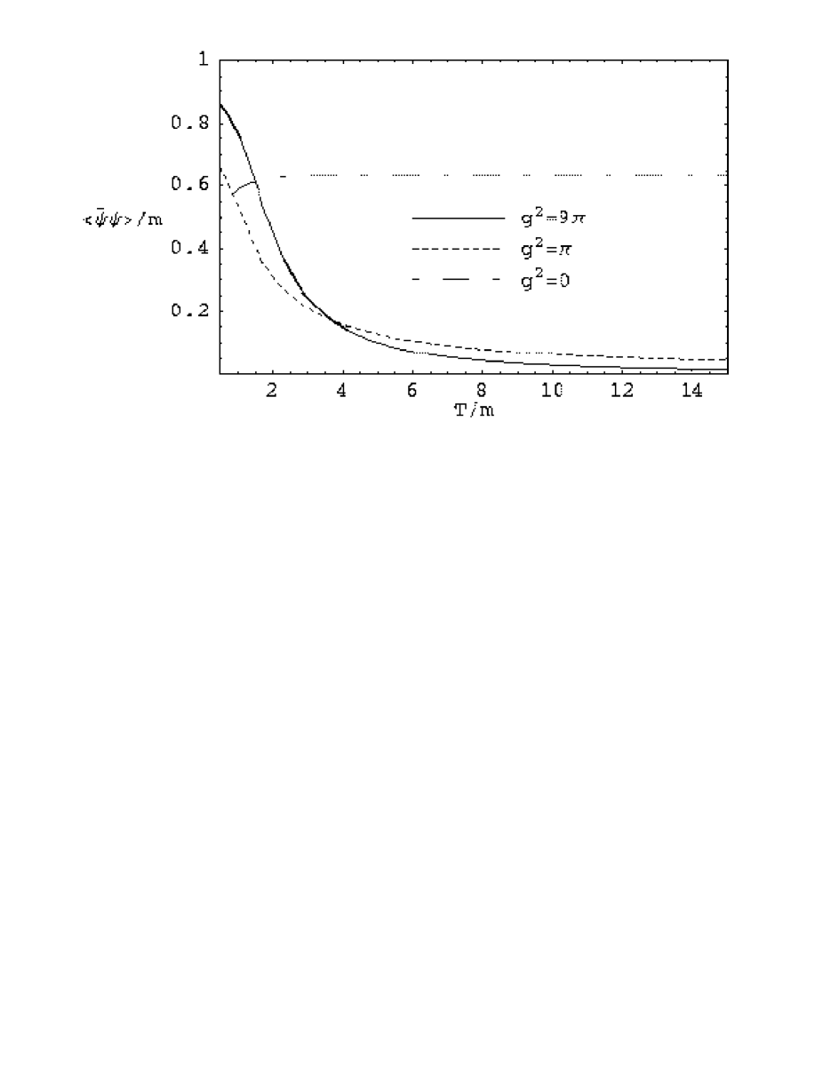
Figure 4: The fermion condensate as a function of temperature in units of $m$, for different values of $g^{2}$

From the above discussion the following picture emerges: for large values of $g^{2}$, the system at high temperatures behaves like a gas of neutral “molecules” made of pairs of chiral charges (chiral neutrality) and the chiral symmetry tends to be restored continuously (i.e, no phase transition) and asymptotically as $T$ increases. As we decrease $g^{2}$, the “molecule” phase tends to disappear in favour of the “plasma” phase—as was already seen for the pressure. Here the $\sigma_{+}$ and $\sigma_{-}$ correlators can be different from zero in chiral non-invariant combinations and thus the chiral symmetry remains broken even for large temperature.

Consequently if we look now at the two-point correlators, we should see a tendency of the system to increase the $\sigma_{+}\sigma_{-}$ correlator against the $\sigma_{+}\sigma_{+}$ one in the “molecule” phase, i.e, for high temperatures and large enough $g^{2}$. That will be the purpose of the next section.

4.2 Two-charge correlators and the screening length

Let us begin by recalling the definition of the two-charge density functions in the Coulomb gas [17]:

$$f_{+-}(X,Y) = \frac{1}{\Omega}\sum_{N=1}^{\infty}\frac{z^{2N}}{(N!)^{2}}\left(\prod_{i=1}^{2N}\int_{0}^{L}dq_{i}\right)\sum_{i=1}^{N}\sum_{j=N}^{2N}\delta(q_{i}-X)\delta(q_{j}-Y)$$ (4.6)

$$\times \exp\left[2\pi\sigma^{2}\theta^{-1}\sum_{1\leq j<i\leq 2N}\epsilon_{i}\epsilon_{j}|q_{i}-q_{j}|\right]$$

$$= \frac{1}{\Omega}\sum_{N=1}^{\infty}\frac{z^{2N}}{((N-1)!)^{2}}\left(\prod_{i=1}^{2N}\int_{0}^{L}dq_{i}\right)\delta(q_{N}-X)\delta(q_{2N}-Y)$$

$$\times \exp\left[2\pi\sigma^{2}\theta^{-1}\sum_{1\leq j<i\leq 2N}\epsilon_{i}\epsilon_{j}|q_{i}-q_{j}|\right],$$

$$f_{++}(X,Y) = \frac{1}{\Omega}\sum_{N=2}^{\infty}\frac{z^{2N}}{(N!)^{2}}\left(\prod_{i=1}^{2N}\int_{0}^{L}dq_{i}\right)\sum_{i=1}^{N}\sum_{i\neq j=1}^{N}\delta(q_{i}-X)\delta(q_{j}-Y)$$ (4.7)

$$\times \exp\left[2\pi\sigma^{2}\theta^{-1}\sum_{1\leq j<i\leq 2N}\epsilon_{i}\epsilon_{j}|q_{i}-q_{j}|\right]$$

$$= \frac{1}{\Omega}\sum_{N=2}^{\infty}\frac{z^{2N}}{N!(N-2)!}\left(\prod_{i=1}^{2N}\int_{0}^{L}dq_{i}\right)\delta(q_{N-1}-X)\delta(q_{N}-Y)$$

$$\times \exp\left[2\pi\sigma^{2}\theta^{-1}\sum_{1\leq j<i\leq 2N}\epsilon_{i}\epsilon_{j}|q_{i}-q_{j}|\right].$$

As in the single charge case, the above functions depend only on $X-Y$ in the $L\rightarrow\infty$ limit (translation invariance). Also, notice that $f_{-+}=f_{+-}$ and $f_{--}=f_{++}$ while for brevity we have omitted the dependences on $z,\theta,\sigma,L$. Our task now will be to compare (4.6)-(4.7) with the MT correlators at finite temperature; $\ll\sigma_{+}\sigma_{-}\gg$ and $\ll\sigma_{+}\sigma_{+}\gg$ respectively. Let us start with the $+-$ correlator. In [3], the following result was obtained:

$$\ll T_{C}\sigma_{+}(X)\sigma_{-}(Y)\gg = \frac{Z_{0}^{F}(T)}{Z_{MT}(T)}\left(\frac{T}{\rho}\right)^{\lambda^{2}/2\pi}\left(\frac{\rho}{2}\right)^{2}\sum_{n=0}^{\infty}\left(\frac{1}{n!}\right)^{2}\left[\frac{\rho\,m}{2}\left(\frac{T}{\rho}\right)^{\lambda^{2}/4\pi}\right]^{2n}$$ (4.8)

$$\times \prod_{j=1}^{2(n+1)}\int_{0}^{\beta}d\tau_{j}\int_{0}^{L}dq_{j}\delta^{(2)}(x_{n+1}-X)\delta^{(2)}(x_{2n+2}-Y)$$

$$\times \prod_{k<j}\left[Q^{2}(x_{j}-x_{k})\right]^{\epsilon_{j}\epsilon_{k}\lambda^{2}/4\pi}$$

where $\epsilon_{j}=+$ for $j=1,\dots,n+1$, $\epsilon_{j}=-$ for $j=n+2,\dots,2n+2$ and $T_{C}$ means contour ordering along $C=[0,-i\beta]$. For convenience we have retained $\lambda$ in the exponents rather than $g$. Again, the above correlator depends only on $X-Y$ in the thermodynamic limit. Notice that we are using the same notation $X$ and $Y$ both for one-dimensional and two-dimensional variables; the meaning should become clear from the context.

As for the $\sigma_{+}\sigma_{+}$ correlator, it can be calculated through the same procedure followed in [3] for the $+-$ correlators using the generating functional technique. Notice that this correlator is not chiral invariant, unlike the $\sigma_{+}\sigma_{-}$ one, which makes its analysis slightly more involved, as explained in [3]. Despite that, we obtain after renormalisation

$$\ll T_{C}\sigma_{+}(X)\sigma_{+}(Y)\gg = \frac{Z_{0}^{F}(T)}{Z_{MT}(T)}\left(\frac{T}{\rho}\right)^{\lambda^{2}/2\pi}\left(\frac{\rho}{2}\right)^{2}\sum_{n=0}^{\infty}\frac{1}{n!(n+2)!}\left[\frac{\rho\,m}{2}\left(\frac{T}{\rho}\right)^{\lambda^{2}/4\pi}\right]^{2n+2}$$ (4.9)

$$\times \prod_{j=1}^{2(n+2)}\int_{0}^{\beta}d\tau_{j}\int_{0}^{L}dq_{j}\delta^{(2)}(x_{n+2}-X)\delta^{(2)}(x_{n+1}-Y)$$

$$\times \prod_{k<j}\left[Q^{2}(x_{j}-x_{k})\right]^{\epsilon_{j}\epsilon_{k}\lambda^{2}/4\pi}$$

where $\epsilon_{j}=+$ for $j=1,\dots,n+2$, $\epsilon_{j}=-$ for $j=n+3,\dots,2n+4$.

Note that the ratio

$$R(\lambda,T;X)=\frac{\ll T_{C}\sigma_{+}(X)\sigma_{-}(0)\gg}{\ll T_{C}\sigma_{+}(X)\sigma_{+}(0)\gg}$$

is scale invariant—this is the observable in which we are interested. However, before proceeding further, we need to clarify how DR works for the above correlators. We begin by noting that DR is not allowed for all values of $X-Y$ in (4.8)-(4.9). In fact, performing the $\delta^{(2)}$ integrations, a factor $[Q^{2}(X-Y)]^{\pm\lambda^{2}/4\pi}$ comes outside the integrals and it is clear that the replacement (2.4) will be allowed for that factor only for $q\gg\beta/2\pi$, where $q$ is the spatial component of $X-Y$. Besides, our analysis for the partition function does not imply that even inside the integrals in (4.8)-(4.9) such replacement can be done. The detailed analysis (which follows a similar line to that of sections 2.1 and 2.2) can be found in the appendix. Here we simply summarise the result: the structure of the correlators (4.8)-(4.9) makes it possible to reduce them dimensionally (inside the integrals) in the large $g^{2}$ (small $\lambda$) limit but not in the large $T$ one. If, in addition one works at large distances $q\gg\beta/2\pi$, the the $Q$’s outside the integrals are also dimensionally reduced. Bearing this in mind, we shall proceed to evaluate these correlators in the dimensionally reduced regime by exploiting again the analogy with the Coulomb gas.

4.2.1 Two-point correlators and the Coulomb gas

Given the conditions for DR to work for the correlators, let us now compare (4.8) with (4.6) and (4.9) with (4.7). For that purpose we replace the $Q$’s inside the integrals in (4.8) by their asymptotic values (2.4). In doing so, we have to remember that such replacement is not allowed in general for the term $j=n+1$, $k=2(n+1)$ (see the above comment). Next, shift $n\rightarrow n-1$ in the sum so that, comparing with (4.6), we get

$$\ll T_{C}\sigma_{+}(X)\sigma_{-}(0)\gg = \left(\frac{1}{4}\right)^{\lambda^{2}/4\pi}\frac{T^{2}}{m^{2}}\frac{e^{\lambda^{2}q/2\beta}}{\left[Q^{2}(q,\tau)\right]^{\lambda^{2}/4\pi}}$$

$$\times f_{+-}\left(z=\frac{m^{2}}{2T}\left(\frac{2T}{m}\right)^{\lambda^{2}/4\pi},\theta=T,\sigma=\frac{\lambda T}{\sqrt{4\pi}};q\right),$$

where $X=(q,\tau)$, we have set $Y=0$ and we have also made use of (3.2). It is important to point out that the overall factor $T^{2}/m^{2}$ depends on $\rho$ implicitly through $m$ but does not have explicit $\rho$ dependence (we cannot fix $\rho$ for that factor), whereas the rest—i.e. the function $f_{+-}$—is scale independent and we have fixed $\rho=m$ only in that part.

Following the same steps for the $++$ correlator we now find

$$\ll T_{C}\sigma_{+}(X)\sigma_{+}(0)\gg = 4^{\lambda^{2}/4\pi}\frac{T^{2}}{m^{2}}\frac{\left[Q^{2}(q,\tau)\right]^{\lambda^{2}/4\pi}}{e^{\lambda^{2}q/2\beta}}$$

$$\times f_{++}\left(z=\frac{m^{2}}{2T}\left(\frac{2T}{m}\right)^{\lambda^{2}/4\pi},\theta=T,\sigma=\frac{\lambda T}{\sqrt{4\pi}};q\right)$$

and therefore the scale-independent ratio of the two yields

$$R(\lambda,T;X)=2^{-\lambda^{2}/\pi}\frac{e^{\lambda^{2}q/\beta}}{\left[Q^{2}(q,\tau)\right]^{\lambda^{2}/2\pi}}\frac{f_{+-}\left(z=\frac{m^{2}}{2T}\left(\frac{2T}{m}\right)^{\lambda^{2}/4\pi},\theta=T,\sigma=\frac{\lambda T}{\sqrt{4\pi}};q\right)}{f_{++}\left(z=\frac{m^{2}}{2T}\left(\frac{2T}{m}\right)^{\lambda^{2}/4\pi},\theta=T,\sigma=\frac{\lambda T}{\sqrt{4\pi}};q\right)}.$$ (4.10)

Once more, the main advantage of comparing with the Coulomb gas is that the functions $f_{++}$ and $f_{+-}$ can be calculated exactly. They can also be related with the Mathieu equation (3.3) as [17]:

$$f_{+\pm}(z,\theta,\sigma;q)=\left(\frac{2\pi\sigma^{2}}{\theta}\right)^{2}\sum_{m=0}^{\infty}B_{m}^{+}B_{m}^{\pm}e^{-\left[\gamma_{0}(\hat{z})-\gamma_{m}(\hat{z})\right]\hat{q}}.$$

Here

$$B_{m}^{\pm}=\hat{z}\int_{-\pi}^{\pi}d\phi\;y_{0}(\phi)y_{m}(\phi)e^{\pm i\phi},$$

the $L\rightarrow\infty$ limit has been taken, $\hat{z}=\theta z/2\pi\sigma^{2}$, $\hat{q}=2\pi\sigma^{2}q/\theta$ and $y_{m}(\phi)$, $\gamma_{m}$ are, respectively, the eigenfunctions and eigenvalues of (3.3), with $\gamma_{m-1}>\gamma_{m}$, $m=1,2,\dots$.

First, note that since $\gamma_{m}<0$ for $m\geq 1$ and $\gamma_{0}>0$, only the $B_{0}$ term survives in the above sum in the limit $q\rightarrow\infty$. Then, since $y_{0}(\phi)=y_{0}(-\phi)$, we have $f_{+\pm}\rightarrow(B_{0})^{2}$ in that limit. In fact $B_{0}=\hat{z}\gamma_{0}^{\prime}(\hat{z})$. Since in that limit we can also dimensionally reduce the $Q^{2}$ factors in (4.10), we get

$$R(\lambda,T;q\rightarrow\infty,\tau)=1.$$

After conversion to $g$, our results for $R(g,T;X)$ are plotted in Figure 5 for different values of $T$ and $g^{2}$. In all those curves, we have considered values $q\gg(2\pi T)^{-1}$, so that we can neglect the $\tau$ dependence and thus (4.10) becomes just the ratio $f_{+-}(q)/f_{++}(q)$. We also recall that the $f_{++}$ function can take negative values for smaller $q$, but we have only displayed in Figure 5 the region where $R(T,g;q)$ is positive.

Let us define the parameter $q_{0}$ to be the mean inter-particle distance so that $q_{0}=1/f_{+}$, i.e. the inverse of the density of charges, regardless of whether they are positive or negative. Thus,

$$q_{0}(\lambda,T)=\frac{2T}{m\ll\overline{\psi}\psi\gg}$$

with $m\ll\overline{\psi}\psi\gg$ in (4.5).

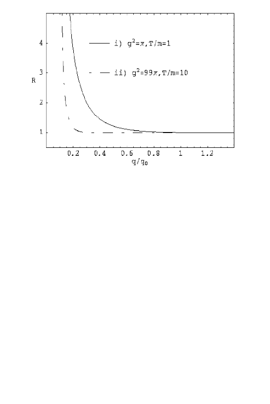
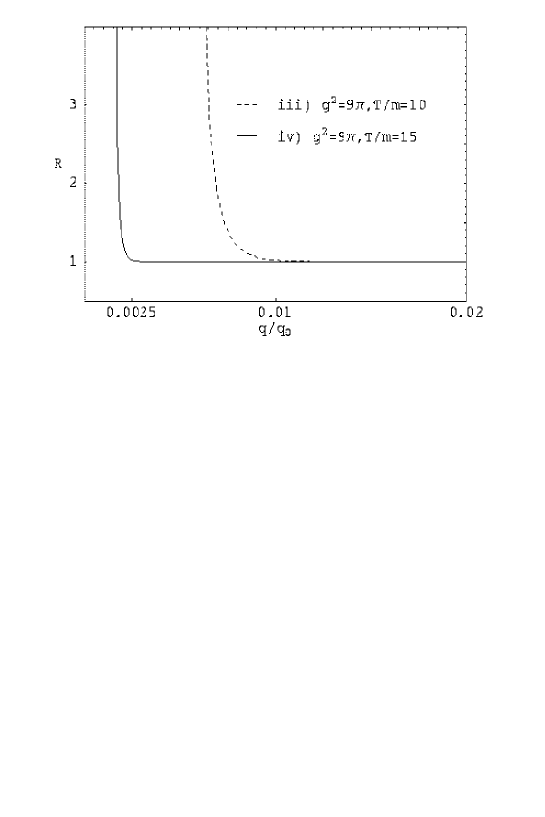
Figure 5: The two-point correlator ratio $R(T,g;q)$ for different values of $T$ and $g^{2}$. The numerical parameters for the above curves are: i)$\hat{z}=0.225$, $(2\pi T)^{-1}/q_{0}=0.044$, ii) $\hat{z}=0.082$, $(2\pi T)^{-1}/q_{0}\simeq 1.3\times 10^{-4}$, iii) $\hat{z}=0.01$, $(2\pi T)^{-1}/q_{0}=2.3\times 10^{-5}$, iv) $\hat{z}=0.005$, $(2\pi T)^{-1}/q_{0}=5\times 10^{-6}$.

As in our previous analysis of the pressure and the fermion condensate, the relevant parameter here is $\hat{z}$ in (3.8). For very small $\hat{z}$ the system is in the condensed regime. Since we need to work at large $g^{2}/\pi$ for DR to work, small $\hat{z}$ means large $T$. In that regime, the $+-$ correlator is much larger than the $++$ one at short distances (but yet large distances compared to $(2\pi T)^{-1}$), as a result of the tendency of the system to form $\sigma_{+}\sigma_{-}$ pairs (“molecules”). For large distances, $R$ tends to 1. In the “normal” phase, i.e, when no “molecules” are formed, we expect that $R$ starts approaching its asymptotic value near $q=q_{0}$ and it does not grow very much below $q_{0}$. Conversely in the “molecule” phase, $R$ grows for small $q$ and it approaches 1 much faster, defining a certain $q_{cond}\ll q_{0}$, which we interpret as the screening length or “molecule” size. For the curves plotted in Fig.5, we get i) $q_{cond}\simeq 1.3q_{0}$, ii) $q_{cond}\simeq 0.3q_{0}$, iii) $q_{cond}\simeq 0.01q_{0}$, iv) $q_{cond}\simeq 0.0025q_{0}$. One can clearly observe that the screening length decreases with the temperature.

5 Dimensional reduction of the Thirring model at nonzero fermion chemical potential

In [3], the issue of thermal bosonisation in the MT/SG system was also studied for $\mu\neq 0$, where $\mu$ is the fermion chemical potential associated with the conservation of the fermion number density $\bar{\psi}\gamma_{0}\psi$ in the Thirring model (the conserved quantity is the number of fermions minus antifermions). It has been shown that the SG model Lagrangian acquires an extra topological term, interpreted as $\mu$ times the number of kinks minus antikinks. The purpose of this section is to show that in the DR regime, the partition function of the Thirring model at $T>0$ and $\mu\neq 0$ can also be related with the 1D Coulomb gas.

We start by recalling the result (in perturbation theory in $m$) obtained in [3] for the partition function of the MT model at $T>0$ and $\mu\neq 0$:

$$Z_{MT}(T,\mu;L)=Z_{m=0}(T,\mu;L)Z_{C}(T,\mu;L)$$

where $Z_{m=0}(T,\mu;L)$ is the massless Thirring result derived in [5] and is given by

$$Z_{m=0}(T,\mu;L)=Z_{0}^{F}(T,L)\exp\left[\beta L\frac{\mu^{2}}{2(\pi+g^{2})}\right]$$

and

$$Z_{C}(T,\mu;L)=\sum_{n=0}^{\infty}\left(\frac{1}{n!}\right)^{2}\left[\frac{\rho m}{2}\left(\frac{T}{\rho}\right)^{\lambda^{2}/4\pi}\right]^{2n}F_{2n}(\lambda,T,\mu;L).$$ (5.1)

Here

$$F_{2n}(\lambda,T,\mu;L)=\prod_{j=1}^{2n}\int_{0}^{\beta}d\tau_{j}\int_{0}^{L}dq_{j}\prod_{k<j}\left[Q^{2}(x_{j}-x_{k})\right]^{\epsilon_{j}\epsilon_{k}\lambda^{2}/4\pi}\exp\left[i\mu\frac{\lambda^{2}}{4\pi}\sum_{j=1}^{2n}\epsilon_{j}q_{j}\right]$$ (5.2)

and, as in (2.2), $\epsilon_{j}=+1$ for $j\leq n$, $\epsilon_{j}=-1$ for $n<j\leq 2n$. Notice that the above partition function is real, as it should, because of the symmetry of the integrand under the simultaneous relabelling $q_{1}\leftrightarrow q_{n+1}$, $\dots$, $q_{n}\leftrightarrow q_{2n}$.

Once more, we need to analyse the regime in which we can dimensionally reduce the $Q$ variables inside the above integral through (2.4). It turns out that the analysis in this case is much simpler than in the case of the two-point correlators and indeed the conclusion is that DR works in the same regime as for the $\mu=0$ pressure, that is, (2.13). We quickly sketch the argument here: first, for small $\lambda$ one readily notes that the leading order is $\mu$-independent since $\sum_{j}\epsilon_{j}=0$. Second, for large $T$, one arrives to an expression identical to (2.7), with $f_{2}(\lambda)$ in (2.8) replaced now by

$$f_{2}(\lambda,\mu)=\int_{0}^{\infty}dq\int_{0}^{1}d\tau\left[Q^{2}(\beta q,\beta\tau)\right]^{-\lambda^{2}/4\pi}\cos\left[\frac{\beta\mu\lambda^{2}q}{2\pi}\right]$$

whose numerical analysis shows a similar behaviour than $f_{2}(\lambda)$, i.e, its corresponding $\Delta f_{2}(\lambda,\mu)$ remains of ${\cal O}(1)$ for $\lambda^{2}/4\pi\raise 1.29167pt\hbox{$<$\kern-7.5pt\lower 4.30554pt\hbox{$\sim$}}1$ for different values of $\beta\mu$. That is easily understandable by realising that $f_{2}(\lambda,\mu)\leq f_{2}(\lambda)$ and $f_{2}^{asym}(\lambda,\mu)>0$, so that $\Delta f_{2}(\lambda,\mu)\leq f_{2}(\lambda)$, which near $\lambda^{2}\raise 1.29167pt\hbox{$<$\kern-7.5pt\lower 4.30554pt\hbox{$\sim$}}4\pi$ (where the error is bigger) is $f(\lambda^{2}\raise 1.29167pt\hbox{$<$\kern-7.5pt\lower 4.30554pt\hbox{$\sim$}}4\pi)={\cal O}(1)$.

Given therefore that one can work in DR also for $\mu\neq 0$, the $Q$’s in (5.2) may be replaced by (2.4). We then realise that $Z_{C}(T,\mu)$ in (5.1) is now the grand canonical classical partition function of the Coulomb gas, the extra $\mu$-dependent term having exactly the form of a purely imaginary external electric field term added to the Hamiltonian of the system. In fact, note that if we wanted to describe ($N$ positive and $N$ negative) charges on the line not only interacting among themselves with a Coulomb force, but also with an external electric field ${\cal E}$, we should add to the Coulomb Hamiltonian the term

$${\cal H}\rightarrow{\cal H}-\sigma{\cal E}\sum_{i=1}^{2N}\epsilon_{i}q_{i}.$$ (5.3)

However, this is precisely the form of the $\mu$-dependent term in (5.2), so that once the $Q$’s are dimensionally reduced one obtains

$$Z_{C}(T,\mu;L)=\Omega\left(z=\frac{m^{2}}{2T}\left(\frac{2T}{m}\right)^{\lambda^{2}/4\pi},\theta=T,\sigma=\frac{\lambda T}{\sqrt{4\pi}},{\cal E}=\frac{i\mu\lambda}{\sqrt{\pi}};L\right)$$

with $\Omega(z,\theta,\sigma,{\cal E},L)$ the grand canonical partition function of the classical Coulomb gas interacting with an external electric field ${\cal E}$ through (5.3).

The exact calculation of the pressure $P(z,\theta,\sigma,{\cal E})=\lim_{L\rightarrow\infty}\log\Omega/\beta L$ was also performed in [16]. In this case though, the result cannot be expressed in a simple way in terms of Mathieu functions as for $\mu=0$. Now it is given by

$$P_{C}(T,\mu)\equiv\lim_{L\rightarrow\infty}\frac{1}{\beta L}\log Z_{C}(T,\mu;L)=\frac{2\pi T^{2}}{1+g^{2}/\pi}\gamma(\hat{z})$$ (5.4)

where $\hat{z}$ is given in (3.8) and the function $\gamma(\hat{z})$ is defined implicitly as follows. Let $G(z,\gamma,\eta)$ be the following continued fraction:

$$G(z,\gamma,\eta)=\frac{z}{\gamma+2\eta+1-\frac{z}{\gamma+4\eta+4-\frac{z}{\gamma+6\eta+9-\dots}}}$$ (5.5)

where

$$\eta=\frac{{\cal E}}{4\pi\sigma}=i\frac{\mu}{2\pi T},$$

and define

$$\bar{Q}(z,\gamma,\eta)=\frac{1}{\gamma}\left[G(z,\gamma,\eta)+G(z,\gamma,-\eta)\right].$$

Now let $z_{0}(\gamma,\eta)$ be the smallest positive solution to the equation

$$\bar{Q}(z_{0}(\gamma,\eta),\gamma,\eta)=1.$$ (5.6)

Then $\gamma(\hat{z})$ is defined implicitly by identifying $\hat{z}^{2}=z_{0}(\gamma,\eta)$.

First note that for $\mu=0$ the above result reduces to the solution in terms of Mathieu functions we have found in section 3. In that case equation (5.6) defines precisely the condition that the two parameters $\hat{z}$ and $\gamma$ of Mathieu’s differential equation (3.3) should satisfy in order that the solution is $2\pi$ periodic. Therefore for $\mu=0$, we have just $\gamma=\gamma_{0}$. In [16] it was shown that equation (5.6) has always a solution. It is worth mentioning that in our case, due to the purely imaginary character of $\eta$, the convergence of the different integrals analysed in [16] and hence of the continued fraction (5.5) is automatically ensured. This should be contrasted with the real $\eta$ case where $\gamma$ and $\eta$ have to satisfy certain constraints to ensure convergence. In addition, notice that for $\gamma$ real, $\bar{Q}$ in (5.5) is also real, which means that the pressure is real, as it should.

Equation (5.6) can be solved exactly in the asymptotic limit $\hat{z}\ll 1$ and $\gamma\ll 1$, where we know there is condensation into “molecules”. For $z,\gamma\ll 1$, $\bar{Q}(z,\gamma,\eta)$ in (5.5) just becomes

$$\bar{Q}(z,\gamma,\eta)\simeq\frac{2z}{\gamma(1-4\eta^{2})}$$

so that

$$\hat{z}^{2}\simeq\frac{\gamma(\hat{z})}{2}\left[1-4\eta^{2}\right]$$ (5.7)

is the smallest solution to $\bar{Q}=1$ and defines $\gamma(\hat{z})$ in this limit. Therefore, using (5.4), replacing the values for $\hat{z}$ and $\eta$, and eliminating $\lambda^{2}$ for $g^{2}$, we find in the $\hat{z}\ll 1$ limit (condensation regime)

$$P_{C}(T,\mu)\simeq\frac{m^{4}(1+g^{2}/\pi)}{4\pi T^{2}}\left(\frac{2T}{m}\right)^{2(1+g^{2}/\pi)^{-1}}\frac{1}{1+\mu^{2}/\pi^{2}T^{2}}.$$

One can check that for $\mu=0$ the above result reduces to the one we have found in section 3 in that regime. Notice that the pressure not only vanishes for large $T$ ($T\gg m$) but also for large $\mu$ at large $T$ ($\mu\gg T\gg m$). That is, chiral restoration also takes place for large $\mu$ (in the large $T$ limit here). This is confirmed by differentiating the above with respect to $m$ to get the fermion condensate, which clearly vanishes as $\mu\rightarrow\infty$. On the other hand, differentiating the pressure with respect to $\mu$ yields the net averaged fermion density,

$$\rho(T,\mu)=\lim_{L\rightarrow\infty}\frac{1}{L}\ll\overline{\psi}\gamma^{0}\psi\gg\;=\frac{\partial}{\partial\mu}P(T,\mu).$$

Thus, we get for the total fermion density in the condensation regime

$$\rho(T,\mu)=\frac{\mu}{\pi+g^{2}}-\frac{m^{4}(1+g^{2}/\pi)}{2\pi^{3}T^{4}}\left(\frac{2T}{m}\right)^{2(1+g^{2}/\pi)^{-1}}\frac{\mu}{(1+\mu^{2}/\pi^{2}T^{2})^{2}}$$ (5.8)

where the first contribution is the massless result obtained in [5]. The above result for the fermion density deserves some comments. One notes that in (5.8) the Coulomb correction to the massless case is always negative and very small in this regime, since the above result is valid only when $T\gg m$. Therefore as $T\rightarrow\infty$, only the massless contribution remains since the first term is $T$-independent. This is nothing but another signal of chiral restoration for large $T$: in that regime there remain only massless fermion excitations in the thermal bath. The same is true if we take in (5.8) the limit $\mu\gg T$ as commented above. In our picture of chiral condensation, the Coulomb term in (5.8) represents the density of “residual” charges that are not yet paired to form chiral “molecules”.

For arbitrary values of $\hat{z}$, the solution to (5.6) has to be found numerically. First, one truncates the continued fraction (5.5) to a given order, making sure that the difference between successive truncations becomes smaller than a fixed numerical precision (see [22] for details). This procedure is meaningful only if the continued fraction is convergent and indeed, by computing it in this way we check numerically the arguments about convergence discussed above. Then one has to find, also numerically, the smallest positive zero of $\bar{Q}(z_{0},\gamma,\eta)=1$. For that purpose we have used a bisection method. In fact, since our objective is to get the function $\gamma(\hat{z})$, it is simpler to look for the zeroes in $\gamma$ fixing $z_{0}=\hat{z}^{2}$. Besides, we have made use of the asymptotic expression (5.7) to check the answer in the large $\hat{z}$ limit.

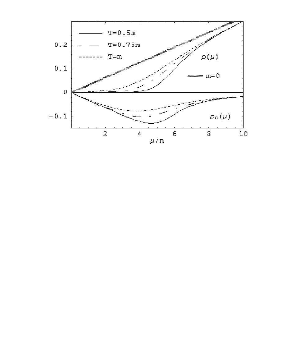
Figure 6: The total net fermion density $\rho(\mu)$ (above the $\mu$ axis) and the Coulomb gas correction $\rho_{C}(\mu)$ to the massless gas (below the axis) for $g^{2}/\pi=9$ and different values of the temperature around $T=m$. The massless result $\rho_{m=0}(\mu)=\mu/(\pi+g^{2})$ is also displayed for $g^{2}/\pi=9$.

Our results for $\rho_{C}(\mu)$ and $\rho(\mu)$ are displayed in figure 6 for temperatures around $T\simeq m$ at fixed $g^{2}/\pi=9$ $(\lambda^{2}/4\pi=0.1)$. When $\hat{z}$ increases, or equivalently when the temperature decreases, $\rho_{C}(\mu)$ (the curves below the axis in figure 6) has a similar shape as that given by the second term in (5.8), but its magnitude increases so that the (negative) correction to the massless gas becomes more and more important. In fact, we see that for $\mu\raise 1.29167pt\hbox{$<$\kern-7.5pt\lower 4.30554pt\hbox{$\sim$}}m$, $\rho_{C}(\mu)$ roughly equals the massless contribution, thus yielding $\rho(\mu)\simeq 0$ in that region, whereas for large $\mu$, $\rho_{C}(\mu)$ becomes negligible and only the massless contribution remains.

In view of this behaviour, let us define two “critical” points: $\mu_{0}\simeq m$ such that $\rho(\mu\raise 1.29167pt\hbox{$<$\kern-7.5pt\lower 4.30554pt\hbox{$\sim$}}\mu_{0})\simeq 0$, $\rho(\mu>\mu_{0})\neq 0$, and $\mu_{1}$ such that $\rho(\mu>\mu_{1})\simeq\rho_{m=0}(\mu)$, where the curve for $\rho(\mu)$ catches up with the massless one, i.e.  $\mu_{1}$ is the chiral restoration point. Recall that we have no true critical behaviour here, so that $\mu_{0}$ and $\mu_{1}$ can be defined only approximately.

Physically, $\mu_{0}$ at $T=0$ would represent the energy needed to excite a fermion in the thermal bath. Thus the behaviour of $\rho(\mu)$ in figure 6 near $\mu=\mu_{0}$ is typical of a massive Fermi gas: It is approximately zero until $\mu\simeq\mu_{0}$. For instance, notice that for a free gas of fermions of mass $m$, $\mu_{0}(T=0)=m$ and $\rho(\mu,T=0)=(\mu-m)\theta(\mu-m)$. For a small but nonzero temperature, that characteristic step-function behaviour is smoothed because there is also thermal energy available, and this can also be observed in figure 6 as $T$ increases. Remember that $T\simeq m$ is the lower temperatures we can take in our DR regime—see our previous comments about the problems with the $T\rightarrow 0^{+}$ limit within our approach. In addition, notice that in our case, the almost exact cancellation between $\rho_{C}(\mu\raise 1.29167pt\hbox{$<$\kern-7.5pt\lower 4.30554pt\hbox{$\sim$}}\mu_{0})$ and $\rho_{m=0}(\mu\raise 1.29167pt\hbox{$<$\kern-7.5pt\lower 4.30554pt\hbox{$\sim$}}\mu_{0})$ for low $T$ takes place after a nontrivial numerical calculation of the Coulomb part, and therefore it provides a good consistency check.

Let us now comment about the behaviour we observe for $\mu>\mu_{1}$ in figure 6. Following our previous description of chiral symmetry restoration in terms of pairing of condensates, our results suggest that the chemical potential also increases the effective “coupling charge” holding the condensate pairs together. In fact, from the viewpoint of the Coulomb gas, we now have another way of increasing the mean potential energy with respect to the mean kinetic energy; namely to switch on a strong electric field $|{\cal E}|\gg T$. It seems natural then that in this regime the systems behaves as in the low temperature phase of Lenard, forming “molecules”. This corresponds to the $\mu>\mu_{1}$ regime in figure 6, i.e. moderate temperatures $T\simeq m$ and large chemical potentials $\mu\gg T$.

As $T$ increases further, the effective mass of the fundamental fermion decreases with $T$, until, for very large $T$, the chiral symmetry is effectively restored and then $\rho(\mu)$ grows linearly with $\mu$ $\forall\mu>0$ as given by (5.8).

This type of behaviour also takes place in QCD at finite baryon density $\rho_{B}$ [24]. There, at $T=0$ one has $\mu_{0}\simeq m_{B}\simeq$ 930 MeV, the vacuum to nuclear matter transition point, with $\rho_{B}(\mu_{0}^{+})\simeq$ 0.16 fm^-3 the density of nuclear matter, and at $\mu_{1}\simeq$ 1300 MeV (for $T=0$) the chiral symmetry is restored (vanishing quark condensate). At both points it is expected that the phase transition is of first order at $T=0$.

Another system where one observes a similar behaviour of $\rho(\mu)$ is the massive Schwinger model [25], where for large $\mu$ the system is in the deconfined phase, unlike the massless case, where there is confinement for any $\mu$ [5].

6 Conclusions

In this paper we have considered the massive Thirring model in 1+1 space-time dimensions at finite temperature $T$ and chemical potential $\mu$. We have shown that in a certain regime, which we have denoted dimensional reduction, the statistical mechanics of this system is the same as that of a classical Coulomb gas in one spatial dimension, where the unit charge grows linearly with the temperature.

The range of validity of the DR regime depends on the observable under consideration: for the pressure, the fermion density and the fermion condensate, we have seen that it works both for $T\gg m$ with $g^{2}>0$ and for $T\raise 1.29167pt\hbox{$>$\kern-7.5pt\lower 4.30554pt\hbox{$\sim$}}m$ with $g^{2}/\pi\gg 1$ (strong coupling regime). However, for the two-point correlators of fermion chiral operators $\sigma_{\pm}(x)$, it only works for large $g$, requiring in addition that the spatial distance $q$ between the two chiral operators is such that $q\gg\beta/2\pi$.

Thanks to the analogy with the Coulomb gas, we have been able to calculate exactly the pressure, fermion density, fermion condensate and two-point correlators of the MT model. Our results show that the chiral symmetry is restored both for high $T$ and high $\mu$ in a continuous way (no phase transition). Chiral symmetry restoration takes place only in the strong coupling (large $g^{2}$) regime. The symmetry restored phase corresponds to the Coulomb “condensed” phase, in which $+-$ pairs of charges tend to pair, forming “molecules”, whereas our low $T$ phase is the Coulomb “plasma” phase, in which the charges are free. The low $T$ and high $T$ behaviours are reversed in our case with respect to the Coulomb gas because the coupling between charges grows with $T$. We have also seen that the rôle of the Coulomb charges is played here by the $\sigma_{\pm}(x)$ operators. These operators tend to pair in the high $T$ or $\mu$ phase forming chiral invariant $\sigma_{+}\sigma_{-}$ combinations. These play the rôle of the “molecules”, whose “size” is determined by the condensation or screening length, which we have estimated for different values of the coupling constant and temperature. We find that the screening length decreases with $T$. In the restored phase, this screening length is of the same order of the inter-particle distance, which is proportional to the inverse of the fermion condensate.

The case of a nonzero fermion chemical potential $\mu$ can also be related to the 1D Coulomb gas, by noting that $\mu$ plays the rôle of a purely imaginary external electric field. For high $T$, the system behaves with $\mu$ as the massless case, which is consistent again with chiral restoration since the effective mass falls off with $T$. For $T\simeq m$, we see that the fermion density is very small until $\mu_{0}\simeq m$ and then starts growing (typical massive Fermi gas behaviour) until eventually, for large $\mu$ ($\mu>\mu_{1}$), it reaches again the massless linear behaviour (chiral restoration). This is again consistent with the idea that the fermion excitation of the system becomes massless both at high $T$ and at high $\mu$. In the case of moderate temperatures, chiral condensates are held together at large $\mu$ by means of the strong external electric field.

Among the analogies with QCD we have found, it is worth mentioning that the chiral condensate vanishes for both large $T$ and $\mu$, although in our case there is no phase transition. In addition, the type of behaviour of the fermion density $\rho(\mu)$ we have obtained at low temperatures is also quite similar to that of the baryon number density $\rho_{B}$ in QCD, where $\mu_{0}$ and $\mu_{1}$ are the vacuum to nuclear matter and chiral restoration critical points, respectively.

Appendix A Dimensional reduction for the two-point correlators

In order to compare the $\sigma\sigma$ correlators (4.8)-(4.9) with the corresponding $ff$ ones ((4.6)-(4.7)) in the Coulomb gas, the former must be dimensionally reduced through (2.4) just as in the case of the partition function. All calculations are performed with respect to $\lambda^{2}$.

Let us start with the $+-$ correlator. The relevant integral to analyse now is:

$$F_{2n}^{+-}(\lambda,T,L;X)=\prod_{j=1}^{2n}\int_{0}^{\beta}d\tau_{j}\int_{0}^{L}dq_{j}\prod_{k<j}\left[Q^{2}(x_{j}-x_{k})\right]^{\epsilon_{j}\epsilon_{k}\lambda^{2}/4\pi}\left[\frac{Q^{2}(x_{j}-X)}{Q^{2}(x_{j})}\right]^{\epsilon_{j}\lambda^{2}/4\pi}$$

where $X\equiv(q,\tau)$, $0\leq q\leq L$ and we have set $Y=0$. The above integral is the counterpart of (2.2). Let us consider first the limit $\lambda^{2}/4\pi\ll 1$. We readily realise that the $X$-dependent factor in the integrand does not contribute to leading order, since $\sum\epsilon_{j}=0$. Thus, following similar steps as in section 2.2, we get

$$\frac{\ll T_{C}\sigma_{+}(X)\sigma_{-}(0)\gg-\ll T_{C}\sigma_{+}(X)\sigma_{-}(0)\gg^{asym}}{\ll T_{C}\sigma_{+}(X)\sigma_{-}(0)\gg}=-\frac{\lambda^{2}}{4\pi}\frac{m^{2}}{2T^{2}}\lim_{\eta\rightarrow\infty}\eta\hat{I}(\eta)+{\cal O}\left(\frac{\lambda^{2}}{4\pi}\right)^{2}$$

where $\hat{I}(\eta)$ is given in (2.9) and the superscript $asym$ means now replacing the $Q$’s inside the integrals as (2.4), but not for the function $Q^{2}(X)$ outside, which would be allowed only for $q\gg\beta/2\pi$ (see our comments in the main text). Notice once more, that one should be careful when taking $T$ to arbitrary small values at the same time as expanding in $\lambda$. Here, we even find a term $m^{2}/T^{2}$ to leading order. Again, we will consider our approach valid only for $T\raise 1.29167pt\hbox{$>$\kern-7.5pt\lower 4.30554pt\hbox{$\sim$}}m$.

Our numerical analysis of $\hat{I}(\eta)$ shows that it vanishes much faster than $\eta^{-1}$ as $\eta\rightarrow\infty$, so that we see that for small $\lambda$, DR (for the integrals) is justified. Notice that the above relative error is scale independent, so we have fixed $\rho=m$. That is not true for the correlator (4.8) itself, where there is an explicit $\rho^{2-\lambda^{2}/2\pi}$ overall dependence.

Next, we will discuss the $T\gg m$ case. Following the same steps as for the partition function, we get now

$$\ll T_{C}\sigma_{+}(X)\sigma_{-}(0)\gg=\frac{Z_{0}^{F}(T)}{Z_{MT}(T)}\left(\frac{T}{\rho}\right)^{\lambda^{2}/2\pi}\left(\frac{\rho}{2}\right)^{2}\left[Q^{2}(X)\right]^{-\lambda^{2}/4\pi}$$ (A.1)

$$\times \left\{1+\left[\frac{1}{2}\left(\frac{m^{2}}{T^{2}}\right)^{1-\lambda^{2}/8\pi}\right]^{2}f_{2}^{+-}(\lambda,X)+{\cal O}\left(\frac{m}{T}\right)^{8-\lambda^{2}/\pi}\right\}$$

with

$$f_{2}^{+-}(\lambda,X)=\int_{0}^{1}d\tau_{1}d\tau_{2}\int_{0}^{\eta}dq_{1}dq_{2}\left[\frac{Q^{2}(q_{1}-q,\tau_{1}-\tau)Q^{2}(q_{2},\tau_{2})}{Q^{2}(q_{1}-q_{2},\tau_{1}-\tau_{2})Q^{2}(q_{2}-q,\tau_{2}-\tau)Q^{2}(q_{1},\tau_{1})}\right]^{\lambda^{2}/4\pi}$$ (A.2)

where $X=(q,\tau)$, $q$ has been rescaled $q\rightarrow q/\beta$ and all the $Q^{2}$ functions are evaluated at $\beta=1$. Notice that we have replaced $\rho=m$ in (A.1) only for the scale-independent part, keeping the scale dependence outside the curly brackets.

Thus, for $T\gg m$, we have to analyse the behaviour of the integral (A.2) with $\lambda$ and $X$ or, rather, the difference between $f_{2}^{+-}(\lambda,X)$ and $f_{2}^{+-,asym}(\lambda,X)$ obtained by replacing the $Q$’s by their asymptotic values. Notice that $f_{2}^{+-}(\lambda,0)$ gives exactly the same contribution as the partition function evaluated to the same order, that is, $f_{2}^{+-}(\lambda,0)=f_{2}(\lambda)$ in (2.8). In fact, in the language of Feynman diagrams, this is a disconnected contribution, proportional to $\eta$, so that the factor $Z_{0}/Z_{MT}$ in front ensures that the answer for this correlator is finite as $\eta\rightarrow\infty$ and we take it into account by subtracting the $X=0$ contribution to the correlators. The same is true for $f_{2}^{+-,asym}(\lambda,X)$. Bearing this in mind, let us concentrate on the values of $\lambda^{2}$ close to and below $4\pi$. The reason is twofold: On the one hand, we have seen already that for small $\lambda$ the DR works. On the other hand, those are the values that will give us the biggest contributions to the error, since the integrand of the asymptotic form is not singular at any point, whereas in (A.2), there are singular regions where the denominator vanish, and those give larger (but finite) contributions to the integral the closer we approach to $\lambda^{2}\raise 1.29167pt\hbox{$<$\kern-7.5pt\lower 4.30554pt\hbox{$\sim$}}4\pi$. The direct numerical evaluation of (A.2) is a hard task. However, for $T\gg m$, all we need to show is that the difference with its asymptotic value remains bounded close to $\lambda^{2}\raise 1.29167pt\hbox{$<$\kern-7.5pt\lower 4.30554pt\hbox{$\sim$}}4\pi$. Therefore, let us estimate it by looking only at the biggest contributions, i.e, those of the regions close to the singularities of the integrand. Firstly, in the region $x_{1}\simeq x_{2}$, where $x_{1}=(q_{1},\tau_{1})$ and $x_{2}=(q_{2},\tau_{2})$, we see that the integrand simply tends to its $X=0$ value, and hence that contribution cancels with the partition function. On the other hand, near $x_{2}\simeq X$ or $x_{1}\simeq 0$, the integrand goes like $\left[Q^{2}(X)/Q^{2}(x_{2}-X)Q^{2}(x)\right]^{\lambda^{2}/4\pi}$. Then,

$$f_{2}^{+-}(\lambda,X)-f_{2}^{+-}(\lambda,0)\sim\left[Q^{2}(X)\right]^{\lambda^{2}/4\pi}\left[f_{2}(\lambda)\right]^{2}\qquad\mbox{(dominant contribution)}$$ (A.3)

We have seen in section 2.1 that $|f_{2}(\lambda)-2^{\lambda^{2}/2\pi}/2\lambda^{2}|\raise 1.29167pt\hbox{$<$\kern-7.5pt\lower 4.30554pt\hbox{$\sim$}}1$ for $\lambda^{2}<4\pi$.

As for the asymptotic contribution to the integral (A.2), we can evaluate it explicitly by integrating over the four separate regions on the $(q_{1},q_{2})$ plane according to the different relative signs of $q_{1}-q_{2}$, $q_{1}-q$ and $q_{2}-q$. We obtain in the $\eta\rightarrow\infty$ limit

$$f_{2}^{+-,asym}(\lambda,X)-f_{2}^{+-,asym}(\lambda,0)=\frac{2^{\lambda^{2}/2\pi+1}}{\lambda^{2}}\left\{-\frac{8}{3}q+\frac{2}{\lambda^{2}}\left[e^{\lambda^{2}q/2}+\frac{1}{9}e^{-3\lambda^{2}q/2}-\frac{10}{9}\right]\right\}$$ (A.4)

Therefore, from (A.4), (A.3) and (A.1), we see that the relative error for the two-point $+-$ correlator—which is a scale independent quantity—does not remain bounded at large $T$ for $\lambda^{2}$ close to $4\pi$, unlike the pressure, but it grows arbitrarily large for $q\gg 1$. In particular, taking $\lambda^{2}\raise 1.29167pt\hbox{$<$\kern-7.5pt\lower 4.30554pt\hbox{$\sim$}}4\pi$ and $q\gg 1$ in the above expressions, we find

$$\frac{\ll T_{C}\sigma_{+}(X)\sigma_{-}(0)\gg-\ll T_{C}\sigma_{+}(X)\sigma_{-}(0)\gg^{asym}}{\ll T_{C}\sigma_{+}(X)\sigma_{-}(0)\gg}\simeq c\frac{m^{2}}{T^{2}}\exp[2\pi q]+{\cal O}\left(\frac{m^{2}}{T^{2}}\right)^{2}$$

with $c=(f_{2}(\lambda)^{2}/4-1/\pi^{2})/4$.

Now we turn to the $++$ correlator. As before, we shall start with the limit $\lambda^{2}/4\pi\ll 1$. From (4.9) we have now

$$\ll T_{C}\sigma_{+}(X)\sigma_{+}(Y)\gg = \frac{Z_{0}^{F}(T)}{Z_{MT}(T)}\left(\frac{T}{\rho}\right)^{\lambda^{2}/2\pi}\left(\frac{\rho}{2}\right)^{2}\sum_{n=0}^{\infty}\frac{1}{n!(n+2)!}\left[\frac{m^{2}}{2}\left(\frac{T}{m}\right)^{\lambda^{2}/4\pi}\right]^{2n+2}$$ (A.5)

$$\times \left[Q^{2}(q,\tau)\right]^{\lambda^{2}/4\pi}F_{2n}^{++}(\lambda,T,X)$$

with

$$F_{2n}^{++}(\lambda,T,X)=\beta^{2(2n+2)}\prod_{j=1}^{2n+2}\int_{0}^{1}d\tau_{j}\int_{0}^{\eta}dq_{j}\left[Q^{2}(x_{j}-X)Q^{2}(x_{j})\right]^{\epsilon_{j}\lambda^{2}/4\pi}\prod_{k<j}\left[Q^{2}(x_{j}-x_{k})\right]^{\epsilon_{j}\epsilon_{k}\lambda^{2}/4\pi}$$

where now

$$\epsilon_{j}=\left\{\begin{array}[]{ll}+&j=1,\dots,n\\ -&j=n+1,\dots,2n+2\end{array}\right.$$

and, as before, we have set $q\rightarrow q/\beta$, $\rho=m$, in the scale-independent part, $X=(q,\tau)$ with $0\leq q\leq\eta$ and the $Q$’s in the integrand are evaluated at $\beta=1$. Notice that now $\sum_{j}\epsilon_{j}\neq 0$, so that we find an additional contribution when expanding in $\lambda^{2}/4\pi$. We find for the relative error

$$\frac{\ll T_{C}\sigma_{+}(X)\sigma_{+}(0)\gg-\ll T_{C}\sigma_{+}(X)\sigma_{+}(0)\gg^{asym}}{\ll T_{C}\sigma_{+}(X)\sigma_{+}(0)\gg}=\frac{\lambda^{2}}{4\pi}\lim_{\eta\rightarrow\infty}\left[\frac{1}{2}\hat{I}(\eta)-2\hat{I}(\eta,X)\right.$$

$$-\left.\frac{g(z)}{f(z)}\hat{I}(\eta)\right]+{\cal O}\left(\frac{\lambda^{2}}{4\pi}\right)^{2}$$

with $z=m^{2}\eta/T^{2}$,

$$\hat{I}(\eta,X)=\frac{1}{\eta}\left[\int_{0}^{\eta}dq_{1}\int_{0}^{1}d\tau_{1}\log\left[Q^{2}(q_{1}-q,\tau_{1}-\tau)\right]+2\eta\log 2-\pi\eta^{2}+2\pi q(\eta-q)\right]$$

and

$$f(z) = \frac{z}{2}\frac{d}{dz}\left[\frac{2}{z}I_{0}^{\prime}(z)\right]$$

$$g(z) = \left(\frac{z}{2}\right)^{3}\frac{d}{dz}\left[\left(\frac{2}{z}\right)^{2}f(z)\right]$$

In the thermodynamic limit $\eta\rightarrow\infty$, it is easy to check that $\hat{I}(\eta,X)\rightarrow\hat{I}(\eta)$ because of translation invariance, and that $g(z)/f(z)\rightarrow z/2$, so that the relative error for small $\lambda$ tends to zero (for $T\raise 1.29167pt\hbox{$>$\kern-7.5pt\lower 4.30554pt\hbox{$\sim$}}m$). Again, $asym$ means the same as for the $+-$ correlator, i.e, replacing the $Q$’s by their asymptotic values only inside the integrals, but not for the $\left[Q^{2}(q,\tau)\right]^{\lambda^{2}/4\pi}$ factor in (A.5).

Finally, we will consider $T\gg m$ for this correlator. We have now

$$\ll T_{C}\sigma_{+}(X)\sigma_{+}(0)\gg = \frac{Z_{0}^{F}(T)}{Z_{MT}(T)}\left(\frac{T}{\rho}\right)^{\lambda^{2}/2\pi}\left(\frac{\rho}{2}\right)^{2}\left[Q^{2}(X)\right]^{\lambda^{2}/4\pi}$$

$$\times \left[\frac{1}{2}\left(\frac{m^{2}}{T^{2}}\right)^{1-\lambda^{2}/8\pi}\right]^{2}f_{2}^{++}(\lambda,X){\cal O}\left(\frac{m}{T}\right)^{8-\lambda^{2}/\pi}$$

with

$$f_{2}^{++}(\lambda,X) = \int_{0}^{1}d\tau_{1}d\tau_{2}\int_{0}^{\eta}dq_{1}dq_{2}$$

$$\times \left[\frac{Q^{2}(q_{1}-q_{2},\tau_{1}-\tau_{2})}{Q^{2}(q_{1}-q,\tau_{1}-\tau)Q^{2}(q_{2}-q,\tau_{2}-\tau)Q^{2}(q_{1},\tau_{1})Q^{2}(q_{2},\tau_{2})}\right]^{\lambda^{2}/4\pi}$$

Notice that there is an important difference between this correlator and the previous cases we have analysed, namely, that the difference between the actual value and the asymptotic limit shows up already to leading order in the $m/T$ expansion, which is now ${\cal O}(m/T)^{4-\lambda^{2}/2\pi}$ rather than ${\cal O}(1)$. That means that the relative error for the correlator $f_{2}^{++}(\lambda,X)$ starts now at ${\cal O}(1)$, and therefore is not bounded. To check that this is indeed the case, it is enough to take the dominant contribution to the integral by picking up the different poles, as we did before with the $+-$ correlator. One easily finds now

$$f_{2}^{++}(\lambda,X)\sim\left[Q^{2}(X)\right]^{-\lambda^{2}/4\pi}\left[f_{2}(\lambda)\right]^{2}\qquad\mbox{(dominant contribution)}$$

Notice that in this correlator there is no disconnected contribution, which is consistent with the fact that its large $T$ expansion begins at NLO whereas that of the partition function starts at ${\cal O}(1)$. In other words, $f_{2}^{++}(\lambda,X)$ is finite as $\eta\rightarrow\infty$. On the other hand, the asymptotic contribution yields

$$f_{2}^{++,asym}(\lambda,X)=-\frac{2}{\lambda^{2}}\left[2qe^{-\lambda^{2}q}+3\frac{e^{-\lambda^{2}q}}{\lambda^{2}}-4\frac{e^{-\lambda^{2}q/2}}{\lambda^{2}}\right]$$

Therefore, one readily checks that the relative error for $f_{2}^{++}(\lambda,X)$ is indeed ${\cal O}(1)$ for arbitrary $q$, so that we cannot bound it in the $T\gg m$ limit.

Summarising, the structure of the correlators (4.8)-(4.9) makes it possible to reduce them dimensionally in the small $\lambda$ limit but not in the large $T$ one. As commented above, DR will also work for the factors $Q^{2}(X)$ outside the integral in the limit $q\gg\beta/2\pi$.

References

- [1] S.Coleman, Phys. Rev. D11 (1975) 2088.
- [2] D.Delépine, R.González Felipe and J.Weyers, Phys. Lett. B419 (1998) 296.
- [3] A.Gómez Nicola and D.A.Steer, Nucl. Phys. B549 (1999) 409.
- [4] T.H.R.Skyrme, Proc.R.Soc.Lon.A260 (1961) 127.
- [5] R.F.Alvarez-Estrada and A.Gómez Nicola, Phys. Rev. D57 (1998), 3618.
- [6] R.F.Alvarez-Estrada and A.Gómez Nicola, Phys. Lett. B355 (1995) 288; B380 (1996) 491 (Erratum).
- [7] For a review, see the proceedings of “QCD at finite baryon density”, Bielefeld (Germany) in Nucl. Phys. A642 (1998).
- [8] D.J.Amit, Y.Y.Goldschmidt and G.Grinstein, J.Phys A13 (1980) 585-620.
- [9] J.Zinn-Justin, Quantum Field Theory and critical phenomena, Oxford 1990.
- [10] S.Coleman, Comm. Math. Phys. 31 (1973) 259.
- [11] For a review, see A.Dobado, A.Gómez Nicola, A.López-Maroto and J.R.Peláez, Effective lagrangians for the Standard Model, Springer, 1997, and references therein.
- [12] T.S.Evans, A.Gómez Nicola, R.J. Rivers and D.A.Steer, in preparation.
- [13] R.Monaco, International Journal of Infrared and Millimeter Waves, 11 (1990) 533.
- [14] S.Samuel, Phys. Rev. D18 (1978) 1916.
- [15] S. Jaimungal and A.R. Zhitnitsky, hep-ph/9905540.
- [16] A.Lenard, Jour.Math.Phys.2 (1961) 682-693.
- [17] S.F.Edwards and A.Lenard, Jour.Math.Phys.3 (1962) 778-792.
- [18] P.Ginsparg, Nucl. Phys. B170 (1980) 388.
- [19] T.Appelquist and R.D.Pisarski, Phys. Rev. D23 (1981) 2305.
- [20] K.Kajantie, M.Laine, K.Rummukainen and M.Shaposnikov, Nucl. Phys. B458 (1996) 90.
- [21] J.I.Kapusta, Finite-Temperature Field Theory, Cambridge University Press, 1989.
- [22] M.Abramowitz and I.A.Stegun, Handbook of Mathematical Functions, Dover, 1970.
- [23] A.Rebhan, Proceedings of the 5th workshop on Thermal Field Theories and their applications, Regensburg, Germany, hep-ph/9808480.
- [24] M.Stephanov, proceedings of “QCD at finite baryon density”, Bielefeld (Germany), Nucl. Phys. A642 (1998) 90c.
- [25] W.Fischler, J.Kogut and L.Susskind, Phys. Rev. D19 (1979) 1188.