Abstract

In anti-de Sitter (AdS) space, classical supergravity solutions are represented “holographically” by conformal field theory (CFT) states in which operators have expectation values. These 1-point functions are directly related to the asymptotic behaviour of bulk fields. In some cases, distinct supergravity solutions have identical asymptotic behaviour; so dual expectation values are insufficient to distinguish them. We argue that non-local objects in the gauge theory can resolve the ambiguity, and explicitly show that collections of point particles in ${\rm AdS}_{3}$ can be detected by studying kinks in dual CFT Green functions. Three dimensional black holes can be formed by collision of such particles. We show how black hole formation can be detected in the holographic dual, and calculate CFT quantities that are sensitive to the distribution of matter inside the event horizon.

1 Introduction

According to the “holographic principle” [1], quantum gravity in spacetimes with some prescribed asymptotic behaviour can be described by a theory defined on the boundary at infinity. Such a principle implies an enormous reduction in degrees of freedom relative to conventional local quantum field theory in the bulk spacetime. Nevertheless, everyday experience shows that local objects exist in the semiclassical limit. So, in order to accept the holographic principle, it is necessary to understand how such objects are encoded and detected in the holographic dual.

A simple example of holography is the proposed duality between gravity in anti-de Sitter (AdS) spaces and local conformal field theories (CFTs) defined on the AdS boundary [2]. The semiclassical limit in AdS is related to a large central charge limit of the CFT. In this context, classical supergravity probes are described by dual CFT states in which operators have expectation values derived directly from the asymptotic behaviour of fields coupling to the probe [3]. This was used to show a “scale-radius duality” for a variety of bulk sources, and for wavepackets of supergravity fields – the radial position of a bulk probe is encoded in the scale size of the dual expectation values. Dynamical sources for supergravity fields were studied in [4], where the radial position of a source particle following a bulk geodesic was reflected in the size and shape of an expectation-value bubble in the CFT. Other interesting work along these lines was performed in [5]-[11].

The scale-radius duality provides a simple example of the holographic encoding of information about the location and motion of objects in the additional spacetime dimension. However, as we will discuss in Sec. 2, the simple scale-radius relationship is a consequence of an isometry in pure AdS under rescalings of all coordinates. For spacetimes such as black holes which break the isometries, the relationship between bulk position and boundary observables will be more complicated. We will illustrate this point by discussing a dilaton source falling into a BTZ black hole, following Danielsson et.al. [4]. The same phenomenon is apparent in the collision of two particles to form a black hole in [11]; after the particles collide, their radial position is fixed, but the scales in the boundary expectation values continue to evolve.

If a simple scale-radius duality fails, do CFT expectation values still tell us the location of bulk sources? In Sec. 2, we will review the surprising power of the expectation values, and discuss what one can learn about the bulk in general. If we write AdS in the global coordinate system, all the normalizable mode spherical harmonics fall off at the same rate at the spacetime boundary. As a result, expectation values of the dual operators contain all the multipole moments of any bulk solution which is constructed by superposition of these modes. Therefore, such supergravity configurations will be completely determined by the CFT one-point functions.

However, there are distinct supergravity configurations which are identical outside of some region. Examples include spacetimes with spherically symmetric matter distributions, and collections of point particles in $2+1$ dimensions. It is important to describe these examples from the CFT perspective, because they include simple processes of particular interest, such as spherically symmetric collapse to form a black hole. In such cases, CFT expectation values will not resolve distinct bulk configurations. We will argue that there are non-local quantities in the gauge theory that can provide the necessary data.

The core of this paper is the use of the Feynman Green function to extract information about bulk solutions from the CFT. We consider asymptotically ${\rm AdS}_{3}$ spacetimes containing point particles, as this is a particularly tractable example. In Sec. 3, we derive the effect of a stationary particle on the Green function of an operator dual to a scalar field. We compute the Green function by a WKB approximation, relating it to the length of geodesics, and find that the particle’s presence is signalled by a kink in the propagator. In Sec. 4, we show how the motion of particles in ${\rm AdS}_{3}$ is reflected in these kinks.

In ${\rm AdS}_{3}$, the head-on collision of particles produces a BTZ black hole [12] if the combined energy exceeds a certain threshold. We show in Sec. 5 that in the holographic description of this process there are initially two kinks in the CFT Green function, indicating the separate positions of the two particles. The discontinuities approach each other and merge into a single one associated with the final black hole. Remarkably, the kinks are sensitive to the positions of the particles inside the event horizon, until their eventual collision to form a singularity. This supports the assertion that the holographic dual gives a unitary description of processes localized inside a black hole horizon, which should have important implications for information loss. Flat space may be obtained from AdS by taking the length scale ($\ell$) of the spacetime to infinity. The measurement precision required for detecting the separation of two particles increases with $\ell$. In the flat space limit, we find that infinite precision measurements are required in the holographic dual to three dimensional gravity to detect the difference between one and two bulk particles.

We conclude in Sec. 6 by drawing some general lessons from our work and suggesting directions for the future.

2 Classical probes and dual expectation values

In the Lorentzian version of the AdS/CFT correspondence, we must specify both boundary conditions at infinity and initial conditions for the normalizable modes in spacetime. Changing the boundary conditions at infinity corresponds to turning on sources in the dual CFT, while the choice of normalizable modes corresponds to the state [13]. In [3], it was shown that both of these choices will affect the one-point functions of the operators dual to supergravity fields, and the effect of a number of bulk sources on the expectation values was explicitly calculated. Here, we wish to make some general comments, drawing on previously studied examples for support. The expectation value of the CFT operator is essentially given by the asymptotic value of the normalizable modes [13]. In Poincaré coordinates,

$$\langle{\cal O}({\bf x})\rangle=\Delta\,\tilde{\phi}_{n}({\bf x})+c\int d^{d}{\bf x}^{\prime}{\phi_{0}({\bf x}^{\prime})\over|{\bf x}-{\bf x}^{\prime}|^{2\Delta}}.$$ (1)

The first term is the effect of a normalizable mode $\phi_{n}(z,{\bf x})$, behaving as $z^{\Delta}\,\tilde{\phi}_{n}({\bf x})$ as $z\to 0$, and the second term is the effect of a change in the boundary conditions by $\phi_{0}({\bf x}^{\prime})$.

The normalizable modes of scalar fields of mass $m$ in global AdS_d+1 with scale $\ell$ behave as [13]

$$\Phi=e^{-i\omega t}\,Y_{l,\{{\bf m}\}}(\Omega)\,(\cos\rho)^{\Delta}\,(\sin\rho)^{l}\,{}_{2}F_{1}(a,b,c;\cos^{2}\rho),$$ (2)

where the boundary is at $\rho=\pi/2$, $\Delta=(d+\sqrt{d^{2}+4m^{2}\ell^{2}})/2$, and $Y_{l,\{{\bf m}\}}(\Omega)$ denotes spherical harmonics on $S^{d-1}$. The falloff of the modes as $\rho\to\pi/2$ is independent of the angular quantum numbers. Thus, the dual expectation values $\langle{\cal O}(t,\Omega)\rangle$ will determine all the spherical harmonics, and therefore all the multipole moments, of the bulk solution.

This ensures that the expectation values will contain all information about any solution constructed by superposition of the basic modes (2). At infinity, the fields fall off exponentially in proper distance, but the exponential is the same for all modes. Although the bulk fields are themselves minuscule at the boundary, CFT expectation values are given by the finite prefactor to the decaying exponential.

2.1 Scale-radius duality: the power of symmetry

As seen in the examples discussed in [3, 5], and in several subsequent papers, the radial position of supergravity sources in pure AdS is encoded in the dual one-point function in a particularly simple way; radial translation of the source corresponds to a rescaling of the corresponding expectation value. This is called scale-radius duality, and is an example of a general relationship between radial positions and boundary scales [14, 7].

For sources at fixed Poincaré coordinate radial positions, this relation follows because the AdS metric is unchanged by the rescaling

$${\bf x}\to\lambda{\bf x},~{}~{}~{}~{}z\to\lambda z.$$ (3)

Given the solution describing a source at some radial position, we can describe a source at a different radial position by the redefinition (3). The effect on the asymptotic fields, and hence the one-point function, is simply a rescaling of the coordinates [3].

In global AdS, symmetry dictates that a source at the origin is represented by a CFT expectation value which is constant over the boundary sphere. There is an isometry mapping this source to one following any other geodesic in the spacetime. This isometry acts as a conformal transformation in the dual CFT, a fact exploited in [4, 8] to obtain CFT expectation values dual to moving sources in the bulk.

In cases with less symmetry, the story is more complicated. A good example is a point source for the dilaton falling into a BTZ black hole, which was studied by Danielsson et.al. [4] using the method of images and the result for sources in ${\rm AdS}_{3}$. In the lightlike limit, such a particle entering the boundary at $t=0$, produces the asymptotic dilaton field

$$\Phi=\sum_{n=-\infty}^{\infty}{\delta(\phi_{+}+2\pi n)\over\sinh^{\nu+1}[{(r_{+}-r_{-})\over 2}(\phi_{-}-2\pi n)]}+{\delta(\phi_{-}-2\pi n)\over\sinh^{\nu+1}[{(r_{+}-r_{-})\over 2}(\phi_{+}+2\pi n)]},$$ (4)

where $\phi_{\pm}=t\pm\phi$ and $r_{\pm}$ are the horizons. Therefore, the corresponding expectation value is concentrated on the light cones $t=\pm\phi$, as for a single particle in AdS₅ [8]. The sum over $n$ implements the periodic identification of $\phi$ in the BTZ black hole. Simple scale-radius duality fails here, in the sense that the two light cones cross repeatedly; so the scale size goes to zero, e.g. at $t=\pi$, while the particle never returns to the boundary. In fact, the information concerning the location of the particle in the bulk seems to be contained in the amplitude of $\Phi$, which steadily declines in time.

A related example is a pair of particles colliding to form a black hole – the boundary expectation value associated with each particle will continue to evolve independently after the collision, reaching zero scale size at a later time [11]. In this case also, the isometries used above are not available, being broken by the metric in the region to the future of both particles. Consequently, the simple connection between scale size and radial position fails to apply directly.

2.2 Resolving bulk objects with propagators

There are also examples where the CFT expectation values implied by (1) do not fully characterize a semiclassical bulk state. For example, a spherical shell of matter placed at any position within AdS will have the same asymptotic fields and dual 1-point functions. (Requiring the matter distribution to have compact support implies that these objects are not built from the supergravity modes (2), all of which have tails at infinity.) Similarly, the only supergravity data available at infinity about a collection of point particles in ${\rm AdS}_{3}$ is the total mass. So, the dual CFT stress tensor has an expectation value [15, 16, 17], but this is insufficient to count the particles or locate them in spacetime.

Nevertheless, the CFT should somehow encode the difference between these bulk configurations. We wish to identify some CFT quantities that probe the interior of the spacetime and characterize the bulk solutions conveniently. These quantities should be non-local from the CFT perspective, because the scale-radius duality teaches us that locations further inside the spacetime correspond to larger scales in the gauge theory. Wilson loop expectation values are such quantities – they depend on the action of strings that start on the boundary and penetrate the spacetime [18]. We can also use scattering amplitudes for the operators dual to supergravity fields. As we will see, in the WKB approximation the CFT propagator is dominated by bulk geodesics. Since these penetrate the spacetime, they can be used to distinguish bulk configurations with identical asymptotic fields. Recently this approach has been applied to spherical shells of matter in ${\rm AdS}_{5}$ [19], which will be analyzed further in a forthcoming paper involving one of us [20]. In the remainder of this paper we will work out the details of this procedure for resolving point particles in three dimensions.

3 Stationary particles in ${\rm AdS}_{3}$

Global ${\rm AdS}_{3}$ is described by the metric

$$ds^{2}=d\chi^{2}+\sinh^{2}\chi\,d\phi^{2}-\cosh^{2}\chi\,dt^{2}=\left({2\over 1-r^{2}}\right)^{2}(dr^{2}+r^{2}d\phi^{2})-\left({1+r^{2}\over 1-r^{2}}\right)^{2}dt^{2}.$$ (5)

We have set the AdS length scale $\ell$ to one, $\phi$ has a period $2\pi$, time runs between $\pm\infty$ and $0\leq r=\tanh(\chi/2)\leq 1$ is the radial coordinate. Fixed $t$ surfaces have the Poincaré disc geometry, and the dual CFT is defined on the cylinder at the $r=1$ boundary. The mass of ${\rm AdS}_{3}$ may be computed as in [17] to be $M=-1/8G$ and is equal to the ground state energy of the dual conformal field theory [21]. We will introduce point particles into this spacetime and will show that kinks in the propagator for CFT operators in the dual state locate the particle in the spacetime. It is helpful to begin by recasting the computation of CFT correlators from ${\rm AdS}_{3}$ in a language that is convenient for generalization to point particle states.

3.1 ${\rm AdS}_{3}$ geodesics and dual propagators

A generic scalar field of mass $m$ in asymptotically ${\rm AdS}_{3}$ spaces is dual to an operator ${\cal O}$ of conformal dimension $\Delta=1+\sqrt{1+m^{2}}$. We are going to show how the properties of point particles in ${\rm AdS}_{3}$ can be read off from the Green functions of such operators. It is helpful to begin by computing the propagator in the conformally invariant vacuum. We can normalize the operator ${\cal O}$ so that on the Euclidean plane ($ds^{2}=dx_{1}^{2}+dx_{2}^{2}=dr^{2}+r^{2}d\phi^{2}$) its 2-point function is constrained by conformal invariance to be

$$\langle{\cal O}({\bf x}){\cal O}({\bf x}^{\prime})\rangle={1\over|{\bf x}-{\bf x}^{\prime}|^{2\Delta}}={1\over(r^{2}+r^{\prime 2}-2rr^{\prime}\cos\phi)^{\Delta}},$$ (6)

where $r$ and $r^{\prime}$ are the distances from the origin and $\phi$ is the angle between ${\bf x}$ and ${\bf x}^{\prime}$. Transform to the Euclidean cylinder ($ds^{2}=dt^{2}+d\phi^{2}$) by setting $r=e^{t}$ and Weyl rescaling the metric by $e^{-2t}$. Let $-\pi\leq z\leq\pi$ parametrize any closed curve on this cylinder with the condition

$${\bf b}(z)\equiv(t(z),\phi(z))=(t(-z),-\phi(-z))$$ (7)

imposed for later convenience. Then

$$T(z)\equiv\ln\langle\,{\cal O}({\bf b}(z))\,{\cal O}({\bf b}(-z))\,\rangle=-2\Delta\,\ln(\,2\,\sin\phi(z)\,).$$ (8)

Wick rotating to Lorentzian signature ($ds^{2}=-dt^{2}+d\phi^{2}$) leaves (8) unchanged, but in Lorentzian signature it should be understood as the logarithm of the Feynman Green function for ${\cal O}$. We want to reproduce this from the AdS/CFT correspondence in a manner convenient for generalization to point particles in ${\rm AdS}_{3}$.

The CFT dual to ${\rm AdS}_{3}$ is defined on a cylinder with diverging Weyl factor. So the Green function for dual operators at any finite coordinate separation will vanish. It is convenient to regulate this behaviour by cutting off the spacetime at a boundary defined by

$$r_{{\rm m}}(t,\phi)=1-\epsilon(t,\phi),~{}~{}~{}~{}~{}\epsilon(t,\phi)=\epsilon(t,-\phi),$$ (9)

where $\epsilon$ is some smooth function of the boundary coordinates. The symmetry of $\epsilon$ under $\phi\rightarrow-\phi$ is merely chosen to reduce verbiage in the remainder of this paper, and ensures that boundary curves ${\bf b}(z)$ satisfying (7) also satisfy $r_{m}({\bf b}(z))=r_{m}({\bf b}(-z))$. According to [5], the propagator for ${\cal O}$ in the dual CFT is obtained by evaluating the spacetime propagator between the corresponding points on the cutoff boundary at $r_{\rm m}$ (also see [22]). In the limit $\epsilon\rightarrow 0$, we expect the Green function computed this way to scale to zero as the Weyl factor of the boundary metric diverges.

Defining the cutoff boundary curve

$${\bf B}(z)\equiv({\bf b}(z),r_{m}({\bf b}(z))),$$ (10)

the propagator for a scalar field of mass $m$ between points ${\bf B}(\pm z)$ should be given by

$$G({\bf B}(z),{\bf B}(-z))=\int{\cal D}{\cal P}~{}e^{i\Delta\,L({\cal P})}.$$ (11)

(We will always be interested in large masses so that $\Delta\approx m$.) Here we are summing over all particle paths between the two boundary points and $L({\cal P})=\int(-g_{\mu\nu}\dot{X}^{\mu}\dot{X}^{\nu})^{1/2}$ is the proper length of the path. (Defined this way, $L({\cal P})$ is imaginary for spacelike trajectories.) As a check, note that the action accumulated along a stationary trajectory should be $E_{0}t$ where $E_{0}$ is the lowest energy the particle can have. A scalar field of “mass” $m$ in ${\rm AdS}_{3}$ has lowest energy eigenvalue $\Delta$ [13] – so the paths in (11) are weighted by $\exp(i\Delta\,L)$. In the semiclassical WKB approximation, the path integral localizes to its saddlepoints and is given by a sum over geodesics

$$G({\bf B}(z),{\bf B}(-z))=\sum_{g}e^{-\Delta\,L_{g}({\bf B}(z),-{\bf B}(z))}.$$ (12)

Here $L_{g}$ is the (real) geodesic length between the boundary points. According to [5], in the large $N$ limit, (12) is also the CFT propagator.

To check this statement, we will reproduce the known Green function of ${\cal O}$ (8) from (12) in global ${\rm AdS}_{3}$. As discussed by Matschull [23], equal-time geodesics of (5) are circle segments obeying the equation

$$\tanh\chi\,\cos(\phi-\alpha)=\cos(\beta),$$ (13)

where the geodesic reaches the $\chi=\infty$ boundary at $\phi=\alpha\pm\beta$. Setting $\alpha=0$, and cutting off the spacetime at

$$r_{{\rm m}}=\tanh(\chi_{{\rm m}}/2)=1-\epsilon(t,\phi),$$ (14)

the unique geodesic between the boundary points $(t,\pm\beta)$ intersects the cut off boundary at $\phi_{m}^{\pm}$ which are fixed by

$$\tanh\chi_{{\rm m}}\,\cos\phi_{{\rm m}}^{\pm}=\cos(\pm\beta).$$ (15)

Our convenient choice $\epsilon(t,\phi)=\epsilon(t,-\phi)$ implies that

$$-\phi_{m}^{-}=\phi_{m}^{+}\equiv\phi_{m}.$$ (16)

Then the length of a geodesic travelling between $(t,\chi_{{\rm m}},\pm\phi_{{\rm m}})$ is

$$L(\phi_{{\rm m}},-\phi_{{\rm m}})=2\ln\left[\sinh\chi_{{\rm m}}\,\sin\phi_{{\rm m}}+(\sinh^{2}\chi_{{\rm m}}\,\sin^{2}\phi_{{\rm m}}+1)^{1/2}\right].$$ (17)

So, to leading order in $\epsilon(z)\equiv\epsilon({\bf b}(z))$, the geodesic length between the points ${\bf B}(\pm z)$ on the cut off boundary curve is

$$L({\bf B}(z),{\bf B}(-z))=2\ln\left(2\sin\phi(z)\over\epsilon(z)\right).$$ (18)

Using (12) and [5], the CFT propagator and the bulk propagator are equated to give

$$T(z)\equiv\ln G({\bf B}(z),{\bf B}(-z))=-2\Delta\ln\left(2\sin\phi(z)\over\epsilon(z)\right)$$ (19)

in the $\epsilon\rightarrow 0$ limit, where the boundary metric is $ds^{2}=(1/\epsilon(t,\phi)^{2})(-dt^{2}+d\phi^{2})$. This is exactly right from the AdS/CFT perspective since (8) is defined on the Weyl rescaled cylinder $ds^{2}=-dt^{2}+d\phi^{2}$.

3.2 Stationary particles

Stationary point particles are introduced in three dimensional gravity by excising a wedge from the spacetime (5). (For example, see [16, 23] and references therein.) A massive particle can only be stationary in (5) at $r=0$, and leads to the spacetime drawn in Fig. 1. The two coordinate systems displayed in the figure remove different wedges of the Poincaré disc:

$${\rm C1:}~{}~{}~{}~{}~{}\pi+\gamma~{}> \phi >~{}\pi-\gamma,$$

$${\rm C2:}~{}~{}~{}~{}~{}~{}~{}-\gamma~{}< \phi <~{}\gamma.$$ (20)

In both cases the wedge boundaries are identified. The dual CFT is still defined on the boundary at infinity, a cylinder whose spatial circle can always be chosen to have a period $2\pi$ by a coordinate transformation. We would like to know how the presence of the particle is registered in the CFT.

Figure 1: Coordinate systems for a stationary point particle in ${\rm AdS}_{3}$. The region $\pi+\gamma\leq\phi\leq\pi-\gamma$ and $-\gamma\leq\phi\gamma$ are removed in C1 and C2 respectively. The edges of the excised regions are identified.

Since the asymptotic spacetime is locally AdS, local measurements on the spacetime boundary cannot tell us that there is a particle in the interior. Nevertheless, the mass of the particle is available globally – integrating the spacetime stress tensor of [17] over the truncated range of $\phi$ gives

$$M=-{1\over 8G}+{\gamma\over 8\pi G}.$$ (21)

The second term is the contribution of the particle. Equivalently, in the Chern-Simons formulation of three dimensional gravity, the mass of the particle is registered in the holonomy of the Chern-Simons gauge fields [16]. Within the AdS/CFT context, the computation that gives (21) also gives the energy of the dual CFT state. Stationary particle spacetimes exist in the range $0\leq\gamma\leq\pi$ with the associated masses $-1/8G\leq M<0$. The range $M\geq 0$ is occupied by the spectrum of BTZ black holes [12].

If multiple particles are placed in ${\rm AdS}_{3}$, a similar calculation will show that the expectation value of the dual stress tensor yields the total mass of the particles. However, this is not enough data to locate the particles in spacetime or count them. So we seek other ways of detecting point particles in ${\rm AdS}_{3}$. We would like a quantity in the dual CFT that probes the interior of the bulk geometry. The propagator is such an object, since it is determined by bulk geodesics running between boundary points.

Following the pure AdS analysis, consider the coordinate system C1 and cut off the spacetime as in (9). As before, consider closed spacelike curves ${\bf b}(z)$ satisfying (7) on the AdS boundary, and the associated cutoff boundary curve ${\bf B}(z)$ (10). Geodesics running between ${\bf B}(\pm z)$ for small $\phi_{1}(z)$ will not pass through the wedge. Their length is therefore given by the ${\rm AdS}_{3}$ result (18):

$$L({\bf B}(z),{\bf B}(-z))=2\ln\left(2\sin\phi_{1}(z)\over\epsilon(z)\right).$$ (22)

For large $\phi_{1}(z)$, the geodesics will run through the excised wedge. To analyze these trajectories it is convenient transform to coordinates C2:

$$r_{2}=r_{1}~{}~{}~{}~{}~{};~{}~{}~{}~{}~{}t_{2}=t_{1}~{}~{}~{}~{}~{};~{}~{}~{}~{}~{}\phi_{2}=\phi_{1}+\gamma~{}~{}(\phi_{1}>0)~{}~{}~{}~{}~{};~{}~{}~{}~{}~{}\phi_{2}=\phi_{1}-\gamma~{}~{}(\phi_{1}<0).$$ (23)

The geodesics that intersect the identification in C1 are precisely those that miss it in C2 and vice versa. The pure AdS result in C2 gives the length of geodesics passing through the C1 wedge. For some intermediate values of $\phi(z)$ there are two geodesics between the points ${\bf B}(\pm z)$. However, the sum (12) is dominated by the geodesic with shortest, length which we will now focus on.

By symmetry, the endpoints of the minimum length geodesics that do and do not pass through the C1 wedge must be separated by the surface

$$\pm\phi_{1}=\bar{\phi}\equiv{\pi-\gamma\over 2}.$$ (24)

Let $\bar{z}$ be the parameter where $\phi_{1}(z)=\bar{\phi}$ . The geodesics between ${\bf B}(\pm z)$ for $0\leq z\leq\bar{z}$ then foliate a spacelike surface on one side of the particle worldline, while $z\geq\bar{z}$ generates a spacelike surface on the other side. It is easy to check that neither of these surfaces touches the particle worldline, but they meet at the AdS boundary at the angles $\phi_{1}=\pm\bar{\phi}$. Together they sweep out a spacelike surface that cuts through AdS, but has a tear in it which could be filled by a spacelike patch. The worldline of the particle passes through this tear.

In C1 coordinates we then have:

$$0\leq\phi_{1}(z)\leq\bar{\phi}:~{}~{}~{}~{}~{}~{}L({\bf B}(z),{\bf B}(-z)) = 2\ln\left(2\sin\phi_{1}(z)\over\epsilon(z)\right).$$ (25)

$$\bar{\phi}\leq\phi_{1}(z)\leq\pi-\gamma:~{}~{}~{}~{}~{}L({\bf B}(z),{\bf B}(-z)) = 2\ln\left(2\sin(\phi_{1}(z)+\gamma)\over\epsilon(z)\right).$$ (26)

Following the discussion for pure ${\rm AdS}_{3}$,

$$T(z)\equiv\ln G({\bf B}(z),{\bf B}(-z))=-\Delta\,L({\bf B}(z),{\bf B}(-z)).$$ (27)

There is a kink in $T$ at the coordinate $z=\bar{z}$ at which $\phi_{1}(z)=\bar{\phi}$:

$$K=\left[{\partial T\over\partial z}\right]_{\bar{z}^{+}}-\left[{\partial T\over\partial z}\right]_{\bar{z}^{-}}=2\Delta\left({\partial\phi_{1}(z)\over\partial z}\right)_{z=\bar{z}}\tan\left({\gamma\over 2}\right)$$ (28)

So the mass of the particle in the bulk can be determined from the strength of the kink in Green functions of generic scalar operators in the dual CFT state:

$$8\pi GM_{{\rm particle}}=\gamma=2\tan^{-1}\left({K\over 4\Delta(\partial\phi_{1}(z)/\partial z)|_{z=\bar{z}}}\right)$$ (29)

Moral of the story:

The family of geodesics between $\pm{\bf B}(z)$ foliates a spacelike surface that cuts across the bulk spacetime. This surface has a tear in it which surrounds the world-line of the stationary particle at the spacetime origin. The kink in the CFT propagator (28) arises because of the sudden jump between geodesics passing on one side and the other of the particle. In the next section we will use a similar strategy to locate moving particles in ${\rm AdS}_{3}$ by examining the resulting moving kinks in CFT propagators.

4 Moving particles in ${\rm AdS}_{3}$

Boosting the stationary particle above leads to a moving particle spacetime. Following Matschull [23], we parametrize ${\rm AdS}_{3}$ as an SL(2,R) manifold via

$${\bf x}=\cosh\chi\,(\cos t\,{\bf 1}+\sin t\,\gamma_{0})+\sinh\chi\,(\cos\phi\,\gamma_{1}+\sin\phi\,\gamma_{2})\,,$$ (30)

with gamma matrices

$${\bf 1}=\pmatrix{1&0\cr 0&1};~{}~{}~{}~{}\gamma_{0}=\pmatrix{0&1\cr-1&0};~{}~{}~{}~{}\gamma_{1}=\pmatrix{0&1\cr 1&0};~{}~{}~{}~{}\gamma_{2}=\pmatrix{1&0\cr 0&-1}.$$ (31)

Here $(t,\phi,\chi)$ are the same coordinates appearing in (5). A boost along $\phi=0$ is performed by the SL(2,R) transformation

$${\bf x}^{\prime}=u^{-1}\,{\bf x}\,u;~{}~{}~{}~{}~{}u=\cosh(\xi/2)\,{\bf 1}-\sinh(\xi/2)\,\gamma_{2}.$$ (32)

Applying this boost to the C1 and C2 coordinate systems for a stationary particle yields the corresponding descriptions of a moving particle.

The relation between the boosted and stationary (subscript $s$) coordinates is

$$\cosh\chi\,\cos t = \cosh\chi_{s}\,\cos t_{s},$$

$$\cosh\chi\,\sin t = \cosh\chi_{s}\,\sin t_{s}\,\cosh\xi+\sinh\chi_{s}\,\cos\phi_{s}\,\sinh\xi,$$

$$\sinh\chi\,\cos\phi = \sinh\chi_{s}\,\cos\phi_{s}\,\cosh\xi+\cosh\chi_{s}\,\sin t_{s}\,\sinh\xi,$$

$$\sinh\chi\,\sin\phi = \sinh\chi_{s}\,\sin\phi_{s}.$$ (33)

(The last equation is redundant, but is retained for convenience.) The particle that was stationary at the origin is now following the periodic trajectory

$$n\pi\leq t\leq(n+1)\pi:~{}~{}~{}~{}~{}~{}~{}~{}\phi=n\pi,~{}~{}~{}\tanh\chi=(-1)^{n}\,\sin t\,\tanh\xi\,,$$ (34)

with $n$ any integer. The boost in (32) is an isometry and leaves the metric unchanged, but the identifications in (20) take a different form in the new coordinates. In the new C1 and C2 coordinates, $t$ dependent wedges are removed behind and in front of the particle respectively, relative to its motion at $t=0$.

Figure 2: Coordinate systems for a moving point particle in ${\rm AdS}_{3}$. The edges of the excised regions are identified.

For purposes of illustration, we will examine the holographic representation of lightlike particles moving through ${\rm AdS}_{3}$. To obtain such objects, take the limit $m\rightarrow 0,\,\xi\rightarrow\infty$ while keeping $m\sinh\xi=\tan\delta$ fixed. Then, using (33) for the boost (32) and a similar relation for its inverse, the relation between the new C1 and C2 coordinates is:

$$\cosh\chi_{1}\,\cos t_{1} = \cosh\chi_{2}\,\cos t_{2},$$

$$\cosh\chi_{1}\,\sin t_{1} = \cosh\chi_{2}\,\sin t_{2}\left(1+{\tan^{2}\delta\over 2}\right)-{\sinh\chi_{2}\,\cos\phi_{2}\,\tan^{2}\delta\over 2}+\sinh\chi_{2}\,\sin\phi_{2},$$

$$\sinh\chi_{1}\,\cos\phi_{1} = \sinh\chi_{2}\,\cos\phi_{2}\left(1-{\tan^{2}\delta\over 2}\right)+{\cosh\chi_{2}\,\sin t_{2}\,\tan^{2}\delta\over 2}+\sinh\chi_{2}\,\sin\phi_{2},$$

$$\sinh\chi_{1}\,\sin\phi_{1} = \sinh\chi_{2}\,\sin\phi_{2}+\tan\delta\,\cosh\chi_{2}(\sin t_{2}-\tanh\chi_{2}\,\cos\phi_{2}).$$ (35)

In this limit, the worldline of the particle is given by

$$-\pi/2\leq t\leq 0:~{}~{}~{}~{}~{}~{}~{}~{}\phi= -\pi, ~{}~{}~{}\sinh\chi=-\tan t.$$

$$0\leq t\leq\pi/2:~{}~{}~{}~{}~{}~{}~{}~{}\phi= 0, ~{}~{}~{}\sinh\chi=\tan t.$$ (36)

The boundaries of the excised wedge in C1 (C2) map to $\phi_{2}=\pi$ ($\phi_{1}=0$) in C2 (C1). We will be interested in geodesics running between the endpoints $(t_{e},\pm\phi_{e},\chi_{e})$ in either C1 or C2 coordinates with $\sinh\chi_{e}\geq\tan t_{e}$ so that the endpoints are always further towards the AdS boundary than the bulk particle. In C1, there is a geodesic which does not pass through the identification if $\phi_{e}<\bar{\phi}$, where

$$\sin t_{e}-\tanh\chi_{e}\,\cos\bar{\phi}=0.$$ (37)

Similarly, in C2, there is a geodesic which does not pass through the identification if $\phi_{e}>\bar{\phi}$ (in C1, these are the geodesics which do pass through the identification). The surfaces defined by (37) in C1 and C2 coordinates are identical; hence, there is a unique geodesic between any pair of endpoints.

The coordinates (33, 35) have the virtue that constant time slices are simply identifications of the Poincaré disc. However, constant $t_{1}$ and $t_{2}$ slices do not coincide. Worse still, constant $t$ slices have a kink in them – the vector $\partial/\partial\phi$ is discontinuous at the identification. We avoid subtleties by working, as before, on some smooth spacelike slice of the boundary; in C1 coordinates the curve is ${\bf b}(z)=(t_{1}(z),\phi_{1}(z))$ satisfying (7). The smooth cutoff at $r_{m}(t,\phi)$ in (9) translates into $\chi_{1m}(t_{1},\phi_{1})$ in C1. So we have the cutoff boundary curve ${\bf B}(z)=({\bf b}(z),\chi_{1m}(z))$, following (10). Similar expressions in C2 are obtained by the coordinate transformation (35). As the curve ${\bf B}(z)$ passes through the separation surface defined by (37), geodesics between ${\bf B}(\pm z)$ cross over the bulk particle.

Geodesics between $\pm{\bf B}(z)$ that avoid the C1 identification intersect the cut off boundary at $\pm\phi_{1m}$ where, following (15),

$$\tanh\chi_{{\rm 1m}}\,\cos\phi_{{\rm 1m}}=\cos\beta.$$ (38)

These geodesics have a path length (17) in C1 coordinates. The separation condition (37) determines some $\bar{z}$ such that, for $z>\bar{z}$, geodesics between ${\bf B}(\pm z)$ intersect the C1 identification. By construction, these geodesics miss the C2 identification and so have a length (17) in C2 coordinates. Setting

$$s_{1}(z)=\sinh\chi_{1m}(z)\,\sin\phi_{1m}(z);~{}~{}~{}~{}~{}s_{2}(z)=\sinh\chi_{2m}(z)\,\sin\phi_{2m}(z),$$ (39)

we have

$$0\leq z\leq\bar{z}: ~{}~{}~{}~{}L(z)= -2\ln\left[s_{1}(z)+(s_{1}(z)^{2}+1)^{1/2}\right].$$ (40)

$$\bar{z}\leq z\leq\pi: ~{}~{}~{}~{}L(z)= -2\ln\left[s_{2}(z)+(s_{2}(z)^{2}+1)^{1/2}\right].$$ (41)

As already established, $T(z)=-\Delta L(z)$ as $\chi_{m}\rightarrow\infty$. The functions $s_{1}(z)$ and $s_{2}(z)$ are related by the last equation of (35), and, along with the separation condition (37), this shows that

$$s_{1}(\bar{z})=s_{2}(\bar{z})\equiv s(\bar{z}).$$ (42)

So $T(z)$ is a continuous function of $z$. However, the derivative $dT/dz$ is discontinuous at $\bar{z}$. Let

$$K=\left[{dT\over dz}\right]_{\bar{z}^{+}}-\left[{dT\over dz}\right]_{\bar{z}^{-}}=\left[{dT\over ds}\right]_{s(\bar{z})}\,\left[\left({ds_{2}\over dz}\right)_{\bar{z}^{+}}-\left({ds_{1}\over dz}\right)_{\bar{z}^{-}}\right].$$ (43)

Again using (35) and (37), $K$ vanishes only if

$$\left[{d\over dz}(\sin t_{2}(z)-\tanh\chi_{2}(z)\,\cos\phi_{2}(z))\right]_{z=\bar{z}}=0.$$ (44)

This fails since $z=\bar{z}$ is exactly the point where ${\bf B}(z)$ intersects the vanishing locus of the quantity being differentiated. Thus, there is a kink in $T(z)$ at the surface (37) where the geodesics cross over the particle.

Locating the particle:

In the holographic CFT, we can identify the position of the kink with the position of the moving particle in the bulk. The arguments above showed that in C1 coordinates, there is a kink at

$$\cos\phi_{1}(\bar{z})={\sin t_{1}(\bar{z})\over\tanh\chi_{1m}(\bar{z})}$$ (45)

As we remove the cutoff $(\chi_{m}\rightarrow\infty)$, the kink is at $\bar{z}$ where $\cos\phi_{1}(\bar{z})=\sin t_{1}(\bar{z})$. So, recalling (36), we can locate the particle in the bulk at the radial position

$$\phi_{1}(\bar{z})\leq\pi/2: ~{}~{}~{}~{}~{}~{}~{}~{}\sinh\chi =-\tan\left(\phi_{1}(\bar{z})-\pi/2)\right)$$

$$\phi_{1}(\bar{z})\geq\pi/2: ~{}~{}~{}~{}~{}~{}~{}~{}\sinh\chi =\tan\left(\phi_{1}(\bar{z})-\pi/2)\right)\,.$$ (46)

As in Sec. 3, the geodesics running between ${\bf B}(\pm z)$ sweep out a spacelike surface that cuts across the bulk spacetime. For a stationary particle, this surface had a spacelike hole in it through with the particle worldline passed. Here, the surface foliated by the geodesics also has a tear in it that stretches between the two boundary points where the curve ${\bf B}(z)$ intersects the separation surface (37). However, it is readily shown that unlike the stationary case this tear can be patched by a null surface – one edge of the tear is always “later” than the other along a null line. The two sheets on either side of the tear are swept out by geodesics that do and do not pass through the C1 identifications, and each sheet touches the null particle worldline at one point. The formulae (46) locate the radial position of the earlier intersection.

For simplicity, we imposed symmetry conditions like (7) and (9) on our regulated boundary surfaces and on the curve ${\bf b}(z)$. In general, we simply have some closed, spacelike curve on the AdS boundary, which we parametrize in some arbitrary way as ${\bf b}(z)$ with $-\pi\leq z\leq\pi$ . To compute the propagator, we impose some cutoff $\chi_{m}(t,\phi)$, and study geodesics between the points ${\bf B}(\pm z)$ (${\bf B}(z)\equiv[{\bf b}(z),\chi_{m}(z)]$). Each parametrization of the curve leads to a different family of geodesics sweeping out a different surface in spacetime. The lightlike bulk particle will pass through a tear in this surface, touching the edges of the tear. Kinks in the CFT propagators can be used to detect these locations.

Relation to higher dimensions:

In [8], the exact metric describing a lightlike particle in ${\rm AdS}_{d}$ for $d>3$ was constructed. This metric takes the form

$$ds^{2}=ds_{0}^{2}+{pf(\rho)\delta(y_{+})dy_{+}^{2}\over(1+y_{+}y_{-}-\rho^{2})},$$ (47)

where $ds_{0}^{2}$ is the pure ${\rm AdS}_{d}$ metric. That is, the metric is pure ${\rm AdS}_{d}$ except on the surface $y_{+}=0$. If we write this metric in the usual global coordinates, as

$$ds_{0}^{2}=-\cosh^{2}\chi dt^{2}+d\chi^{2}+\sinh^{2}\chi(d\theta^{2}+\sin^{2}\theta d\Omega_{d-3}),$$ (48)

then the surfaces of constant time are generated as surfaces of revolution from a Poincaré disc; that is, the two-dimensional subsurfaces given by choosing a pair of antipodal points on the $S^{d-3}$ are Poincaré discs. We have singled out an axis in (48); assume this is the direction along which the particle falls. Then in (47),

$$y_{+}={\cosh\chi\sin t-\sinh\chi\cos\theta\over 1+\cosh\chi\cos t},$$ (49)

and the Poincaré disc is changed by the addition of a delta-function at

$$\sin t-\tanh\chi\cos\theta=0.$$ (50)

This in turn implies that the expectation value of the CFT stress tensor contains a delta function [8], the location of which, comparing (50) and (37), is exactly analogous to the location of the kink in the CFT propagator we have found in the ${\rm AdS}_{3}$ case.

5 Colliding particles

The techniques developed above for single particles can also be applied to two colliding lightlike particles. When the energy in the collision is low, the result is the single particle spacetime of Sec. 3, but above a certain threshold a black hole is created. The representation of this process in the dual CFT is central to understanding holographic descriptions of gravity. The only data available in the supergravity fields at infinity is the total energy of the particles, and we seek ways of locating and counting them. Again, the propagator for an operator dual to a generic ${\rm AdS}_{3}$ scalar field provides more information. As above, consider a one-parameter family of propagators whose associated geodesics foliate a spacelike surface in the bulk. Prior to the collision we expect the null particle worldlines to pass through tears in this surface. Generically this will lead to two CFT propagator kinks, arising as the bulk geodesics dominating the calculation cross over the particle worldlines. It is possible to have a single kink by choosing a family of propagators whose associated geodesics hop over both particles simultaneously. But such special families have zero measure in the space of possibilities we are considering, and so we will ignore them.

Figure 3: Colliding particles in ${\rm AdS}_{3}$. The edges of the excised regions are identified.

As discussed by Matschull [23], a spacetime containing two particles is derived by excising a wedge for each particle from ${\rm AdS}_{3}$. In the center of mass (COM) frame, particles approaching each other head-on can be displayed as in Fig. 3. Particles A and B enter the spacetime at $t=-\pi/2$ at $\phi=-\pi$ and $\phi=0$ respectively and follow the trajectory $\sinh\chi=-\tan t$ (36) until they collide at $t=0$. In Fig. 3, each particle has a wedge excised “behind” its trajectory – if one particle was removed, the other would be in a C1 coordinate system from the previous section. We are interested in geodesics running between the points $(t_{e},\pm\phi_{e},\chi_{e})$ where $\chi_{e}\rightarrow\infty$. For large (small) $\phi_{e}$, we expect the geodesics to enter the particle A (B) identification while for $\phi_{e}$ in the vicinity of $\pi/2$ both wedges should be avoided. Following the single particle analysis and (37), we arrive at the two separation conditions

$$\sin t_{e}-\tanh\chi_{e}\,\cos\phi_{A}=0;~{}~{}~{}~{}~{}~{}\sin t_{e}-\tanh\chi_{e}\,\cos(\pi-\phi_{B})=0.$$ (51)

At any given $t_{e}$ and $\chi_{e}$, geodesics that start at $\phi>\phi_{A}$ ($\phi<\phi_{B}$) intersect the A (B) identification, while geodesics starting at $\phi_{A}<\phi<\phi_{B}$ pass between the two particles. At $t=0$ the particles meet, and $\phi_{A}=\phi_{B}=\pi/2$.

Again, consider closed spacelike boundary curves ${\bf b}(z)$ satisfying (7) with $-\pi\leq z\leq\pi$. Cut off the spacetime at $\chi_{m}(t,\phi)$ satisfying (9) and define the associated curves ${\bf B}(z)$ (10) on the cut off boundary. The separation conditions (51) determine $z_{A}$ and $z_{B}$ at which geodesics between ${\bf B}(\pm z)$ enter the A and B identifications. Then arguments identical to Sec. 4 show that there are kinks at $z_{A}$ and $z_{B}$. At $t=0$ the two separation surfaces (51) meet and so the two kinks join into a single one.

Locating the particles prior to collision:

In the $\chi_{m}\rightarrow\infty$ limit, (51) shows that the kinks occur at $z_{A}$ and $z_{B}$ satisfying $\cos\phi(z_{A})=\sin t(z_{A})$ and $\cos\phi(z_{B})=\sin t(z_{B})$. We can thus locate the two bulk particles at $\sinh\chi_{A}=\tan(\phi(z_{A})-\pi/2)$ and $\sinh\chi_{B}=-\tan(\phi(z_{B})-\pi/2)$ prior to their collision. The surface swept out by the geodesics between ${\bf B}(\pm z)$ has components foliated respectively by geodesics passing behind A, between A and B, and behind B. Each component is spacelike and they meet at the positions on the AdS boundary where the curve ${\bf B}(z)$ intersects the separation surfaces (51). However, in the bulk of spacetime, the three components are separated by two tears through which the particle worldlines pass. As before, it can be shown that these tears can be patched by a null surface – the tear edges passing between the particles are separated by null lines from the edges passing behind the particles. Each particle worldline touches the edges of a tear, and we have used CFT kinks to locate the radial position of the earlier intersection.

The flat space limit:

Flat space can be obtained from AdS by taking the limit $\ell\rightarrow\infty$ while keeping radial coordinate positions $r=\ell\tanh(\chi/2)$ fixed. (See [24] for discussions of the recovery of flat space from AdS.) In this limit, the proper length between the A and B particles is simply $2r_{A}$ and $\chi_{A}=\chi_{B}\rightarrow 0$. So, the kinks will occur at $\phi(z)\approx\pi/2\pm\chi_{A}$. As $\ell\rightarrow\infty$ the proper length between any two boundary points is diverging. However, since $z_{A}\rightarrow z_{B}$ in this limit, the ratio of the proper length between the locations of the kinks and the proper length of the boundary as whole tends to zero. This is symptomatic of a need for extreme precision in CFT measurements to resolve bulk objects at finite separation in the flat space limit.

Figure 4: (a) Particle collision below threshold,   (b) Evolution after collision below threshold,    (c) Horizon formation above threshold,   (d) Collision above threshold,   (e) Evolution above threshold

Collision below the black hole threshold:

In (35), we derived the spacetime of a lightlike particle by boosting a mass $m$ particle with rapidity $\xi$, while keeping $m\sinh\xi=\tan\delta$ fixed. The parameter $\delta$ is related to the energy of the particle, and it is readily shown that the head-on collision of two particles with $\delta\geq\pi/4$ creates a BTZ black hole [23]. Below threshold, the collision produces the stationary particle spacetime in Sec. 3, which we now analyze.

Figs. 4a and 4b display the creation of a stationary particle. The particles A and B in Fig. 3 enter the spacetime at $t=-\pi/2$ and collide at the origin at $t=0$. After this time the spacetime in 4b is identical to that in Fig. 1, but is presented in skewed coordinates – equal time slices in the two figures do not coincide. The two patches in 4b have identified edges and the single stationary particle S at the tip of the patches follows an oscillatory timelike trajectory that never reaches the spacetime boundary, as appropriate to a massive particle [23]. Prior to the collision, we have shown that there are two kinks in the CFT propagator which approach each other. The kinks arise because the bulk surface foliated by geodesics between ${\bf B}(\pm z)$ has two tears in it surrounding the particle worldlines. At $t=0$, the two tears merge because there are no longer any geodesics passing between the particles. So, as manifest in Figs. 4a and 4b, there is only one kink in the equal-time propagator when $t\geq 0$, arising as the associated geodesics switch between the two identifications. The two-kink to one-kink transition at $t=0$ marks the creation of the joint particle.

5.1 Black hole formation

If the particles have a total mass greater than $1/8G$, they will form a black hole upon colliding. We therefore have an exact metric describing the formation of a black hole. Three different coordinate systems are convenient for describing various aspects of the CFT representation of this process.

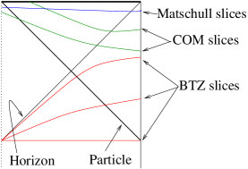
Figure 5: COM, BTZ and Matschull’s BTZ_M slices of a black hole spacetime formed by collision of lightlike particles. The slices are drawn at different times for pictorial clarity. This is not really a Penrose diagram – the mappings between the coordinate systems do not preserve circular symmetry, and so we have simply displayed fixed angle slices in each.

In center of mass (COM) coordinates, the process is shown in Figs. 4c – 4f following [23]. The particles enter the spacetime at $t=-\pi/2$ and follow the trajectory in Fig. 3. At some later time $t=\tau-\pi/2$, an event horizon forms at the thin dashed line in 4c. It grows as the particles approach each other, and the collision at $t=0$ in Fig. 4d creates a spacelike singularity behind the horizon. Successive COM spatial slices for $t>0$ intersect this surface at the point S in Figs. 4d and 4e. As time passes, this point recedes towards the boundary of the Poincaré disc along a spacelike curve. It reaches the boundary at some $t=\tau$ which is the final spacetime point. A picture of COM slices in the global spacetime is shown in Fig. 5. It will transpire that CFT propagators are easiest to compute in these coordinates. However, the spatial slices have a kink in them at the identifications, so they are not entirely natural from the CFT point of view.

Smoother coordinates can be obtained by recalling that the absence of gravitational degrees of freedom implies that even when the particles are separate, the metric far from them can be written in BTZ form [12]:

$$ds^{2}=-N^{2}\,dt_{B}^{2}+r^{2}\,d\phi_{B}^{2}+{1\over N^{2}}\,dr_{B}^{2};~{}~{}~{}~{}N^{2}=r_{B}^{2}-8GM.$$ (52)

The holographic CFT is most naturally described in such coordinates, in which the spacetime boundary is a smooth cylinder. We will construct the colliding particle spacetime in BTZ coordinates by performing surgery on an eternal black hole.

Figure 6: BTZ_M: Poincaré disc coordinates for the BTZ black hole. (A) $t=-\pi/2$, (B) $-\pi/2\leq t\leq 0$, (C) $t=0$

It is convenient to begin with an alternative form of the pure BTZ metric, in which the spatial sections are identifications of the Poincaré disc [23]. Consider global AdS in the coordinates (5) and identify the curves

$$v^{\pm}:~{}~{}~{}~{}\tanh\chi\sin\phi=\mp\sin t\,\tanh\mu$$ (53)

for $-\pi\leq t\leq 0$. The resulting spacetime is displayed in Fig. 6. At $t=-\pi$ we have the collapsed geometry associated with the past singularity. As time passes, an Einstein-Rosen bridge expands between two asymptotically AdS regions. The horizons (thin dashed lines in Fig. 6) come together, meeting at $t=-\pi/2$ in analogy with equal time slices in four dimensional Kruskal coordinates. For $t>-\pi/2$ the Einstein-Rosen bridge collapses again to a future singularity as shown in Fig. 6. We will call these coordinates BTZ_M, while referring to (52) simply as BTZ.

We wish to drop two lightlike particles into ${\rm AdS}_{3}$ at $t=-\pi/2$. Matschull has shown how to present this spacetime in asymptotically BTZ_M coordinates. In Fig. 3 each incoming particle was presented with a wedge removed “behind” its direction of motion (i.e., C1 coordinates from Fig. 2). Now we simply excise a wedge from the BTZ_M spacetime “ahead” of particle B in Fig.  7. The resulting identification intersects $v^{\pm}$ at one point. Particle A is placed at this point, as shown in Fig. 7. In these coordinates, particle B falls in along the trajectory $\phi=0,\tanh\chi=-\sin t$. Near infinity, the spatial slices of this collapsing spacetime are identical to those of the pure BTZ_M black hole in Fig. 6.

Figure 7: BTZ_M  coordinates for colliding particles. (A) The particles enter ${\rm AdS}_{3}$ at $t=-\pi/2$, (B) Both particles are outside the horizon, (C) Both particles are inside the horizon, (D) Collapse to a future singularity at late times

The coordinate transformation between BTZ_M and BTZ coordinates is obtained by relating both to a $(2,2)$ signature flat space in which AdS is embedded as a hyperboloid. This gives

$${r_{B}\over r_{+}}\cosh(r_{+}\phi_{B}) = -\cosh\chi\,\sin t,$$

$${r_{B}\over r_{+}}\sinh(r_{+}\phi_{B}) = \sinh\chi\,\sin\phi,$$

$$\left({r_{B}^{2}\over r_{+}^{2}}-1\right)^{1/2}\cosh(r_{+}(t_{B}+\pi/2)) = \sinh\chi\,\cos\phi,$$

$$\left({r_{B}^{2}\over r_{+}^{2}}-1\right)^{1/2}\sinh(r_{+}(t_{B}+\pi/2)) = \cosh\chi\,\cos t.$$ (54)

Here $r_{+}=\sqrt{8\pi GM}$, and the points $(t,\pm\phi,\chi)$ in BTZ_M correspond to the points $(t_{B},\pm\phi_{B},r_{B})$ in BTZ (with a shift chosen so that $t=-\pi/2$ maps to $t_{B}=-\pi/2$).

The transformation between COM and BTZ coordinates can be found similarly. The equal-time slices of the three coordinate systems do not coincide, and those of COM and BTZ_M have kinks at the identifications. BTZ coordinates only cover the region outside the horizon and are analogous to Schwarzschild coordinates for four dimensional black holes. Conveniently for us, the transformations between the coordinates are symmetric under $\phi\rightarrow-\phi$ – the points $(t,\pm\phi,\chi)$ in one of them is mapped into $(t^{\prime},\pm\phi^{\prime},\chi^{\prime})$ in another.

5.1.1 Detecting particles inside an event horizon

We want to examine families of equal-time propagators as in previous sections to study the CFT representation of black hole formation. As before, consider closed spacelike boundary curves ${\bf b}(z)$ satisfying (7) with $-\pi\leq z\leq\pi$. Cut off the spacetime at $\chi_{m}(t,\phi)$ satisfying (9) and define the associated curves ${\bf B}(z)$ (10) on the cut-off boundary. Then the length of geodesics between ${\bf B}(\pm z)$ as $\chi_{m}\rightarrow\infty$ gives the CFT propagator between ${\bf b}(\pm z)$.

It is easiest to begin in COM coordinates, which we have already studied extensively. Prior to the collision at $t=0$, we have shown above that geodesics between ${\bf B}(\pm z)$ sweep out a bulk surface with two tears in it. One component of this surface passes in between the two particles. As a result, we have shown that the associated CFT Green function has 2 kinks until $t=0$ and that these kinks are related to the positions of the colliding particles. At later times, the colliding particles have formed a spacelike singularity inside the event horizon, and geodesics can no longer pass between them. So, as Figs. 4d and 4e make clear, there is only one kink in the propagator, arising as the associated bulk geodesics switch between the identifications, avoiding the spacetime singularity. In the COM slices with $t>\tau-\pi/2$, the particles are localized inside an horizon; yet, we have just showed that their trajectories affect the CFT propagator until they collide. We have reached a remarkable, and long sought-after [25] conclusion: there are simple quantities in the holographic dual to ${\rm AdS}_{3}$ gravity that are sensitive to the details of the matter distribution inside an event horizon!

The dual CFT is most naturally described on the smooth, cylindrical boundary of conventional BTZ coordinates $\{t_{B},\phi_{B}\}$. So it is interesting to locate kinks in the CFT Green function defined on boundary curves ${\bf b}(z)$ that coincide with synchronous BTZ (52) slices, with the parameter $z$ equated to the BTZ angle ($z=\phi_{B}$). It is helpful to first examine BTZ_M geodesics running between $(t_{e},\pm\phi_{e},\chi_{e})$. For small $\phi_{e}$ the geodesic will pass “behind” particle B and miss the identifications in Fig. 7. For large $\phi_{e}$ the geodesics will pass “behind” particle A and through the $v^{\pm}$ identifications. In an intermediate range of angles, the geodesics will pass between the particles and through the wedge excised from BTZ_M by the particles in Fig. 7. Following our previous analyses, geodesics that pass behind B are separated from those that pass between A and B by the condition

$$\sin t_{e}-\tanh\chi_{e}\cos(\pi-\phi_{e})=0.$$ (55)

We will use (55) to locate kinks in the CFT propagator defined on boundary curves ${\bf b}(z)$ coinciding with synchronous BTZ slices.

The qualitative form of the answer in the limit where the cutoff is removed is clear from the COM discussion of colliding particles. There, (51) gave the location of the kinks, by separating geodesics that do and do not pass through the identifications in Fig. 3 and Fig. 4c. In the $\chi\rightarrow\infty$ limit, this occurs at $\phi_{{\rm COM}}=\pm(t-\pi/2)$ and $\phi_{{\rm COM}}=\pm(t+\pi/2)$, if we drop in particles A and B from $\phi_{{\rm COM}}=-\pi,0$ at $t_{{\rm COM}}=-\pi/2$. That is, the associated kinks travel along lightcones. While the relation between COM and BTZ coordinates is complicated, we expect that in BTZ coordinates, the kinks at infinity should still travel along lightcones.

To see this—and the form of the kink in the cut-off theory— we use the BTZ_M to BTZ transformation (54) and (55) to find the separation condition produced by particle B for BTZ geodesics between $(t_{eB},\pm\phi_{eB},r_{eB})$:

$$\left({r_{eB}^{2}\over r_{+}^{2}}-1\right)^{1/2}\cosh(r_{+}(t_{eB}+\pi/2))={r_{eB}\over r_{+}}\cosh(r_{+}\phi_{eB}).$$ (56)

By symmetry the condition for particle A is

$$\left({r_{eB}^{2}\over r_{+}^{2}}-1\right)^{1/2}\cosh(r_{+}(t_{eB}+\pi/2))={r_{eB}\over r_{+}}\cosh(r_{+}(\phi_{eB}-\pi)).$$ (57)

When we remove the cutoff by taking $r_{e}\rightarrow\infty$, the logic of previous sections shows that the CFT propagator on the BTZ cylinder has kinks at $\phi_{B}=\pm(t+\pi/2)$ and $\phi_{B}=\pm(t-\pi/2)$ as argued above. The kinks move towards each other and meet when $t_{B}=0$ at $\phi_{B}=\pm\pi/2$.

As in previous sections, the family of geodesics is sweeping out some bulk surface. At early times, the surface intersects each particle worldline, producing two CFT kinks. BTZ coordinates (52) are analogous to 4d Schwarzschild coordinates, and only cover the region outside the event horizon. Hence, in these coordinates, we never see the particles cross the horizon and collide. Nevertheless, geodesics between some $(t_{B},\pm\phi_{B})$ must go out of the BTZ patch and penetrate the horizon, since we know that geodesics between COM boundary points $(t,\pm\phi)$ can penetrate the horizon and these are mapped onto some $(t_{B},\pm\phi_{B})$. The endpoints of the geodesics which do this are to the past of the merging of CFT kinks in BTZ coordinates. This is possible because the associated geodesics do not remain at fixed time. They can bend into the future and some of them penetrate the horizon, passing through the BTZ slices to the future in the region the post-kink geodesics skip over. The two CFT kinks for $t<0$ reflect where the surface foliated by the geodesics intersects the particle worldlines, inside or outside the event horizon. At late BTZ times, the geodesics no longer intersect these worldlines. The kink in the CFT propagator then arises because of lensing by the BTZ geometry – the surface swept out by the associated geodesics skips over the throat in the geometry, and the resulting tear is responsible for the CFT kink. If we consider a pair of particles that miss each other and don’t form a black hole, the kinks will approach each other at $t=0$ and then separate again, returning to $\phi=0,\pi$ at $t=\pi/2$. This will happen because evolution in the gauge theory is causal, so differences should only appear in regions that can receive signals from both particles.

6 Discussion

In this paper we have continued an ongoing discussion of the holographic encoding of semiclassical gravitational backgrounds. We have learned some general lessons about the holographic AdS/CFT correspondence. The expectation values of CFT operators contain enough information to completely characterize bulk solutions in a wide variety of circumstances. However, the relationships between CFT expectation values and radial positions of bulk objects can be complicated. Furthermore, localized objects that are not built out of mode solutions to the supergravity equations will be hard to characterize using the expectation values of operators dual to supergravity fields.

We argued that non-local CFT quantities, such as the propagator, can resolve such localized objects and, as an example, studied collections of point particles in ${\rm AdS}_{3}$. We have shown that although the asymptotic supergravity fields only contain data about the total mass of the particles, the CFT Green function is able to enumerate and locate them. Related statements apply to spherical shells in ${\rm AdS}_{5}$ [19, 20]. In both of these cases, the localized object in the bulk has co-dimension one. This is why the bulk geodesics associated with the Green function are sufficient to characterize it – the geodesics probe the one extra dimension that is is not occupied by the object, thereby locating it in that dimension. Similarly, we might expect that objects of co-dimension $n$ can be located in spacetime by transition amplitudes with $(n+1)$ particles.

One aim of this paper was to characterize the different states of a holographic theory describing distinct bulk gravity solutions with identical asymptotic fields. We identified a CFT quantity which depends on the bulk solution in the interior, but the story is far from complete – the “propagator probe” that we have used is not fine-grained enough to resolve many questions of interest, particularly in dimensions higher than 3. We also expect that there will not always be a unique gauge theory state associated with a classical bulk solution (for example, there should be $e^{A/4}$ states ‘associated’ with a spacetime containing a black hole). Our techniques do not shed additional light on this issue.

In our approach, the process of black hole formation is visible in a reduction in the number of kinks in CFT Green functions. Remarkably, the CFT propagator is sensitive to the distribution of matter in the interior of an event horizon. In fact, our analysis of the collision to form a black hole does not differ very much from collision to form a stationary particle, until the singularity forms.

Note that the particles we used to form the black hole play a key role in allowing us to explore its interior; the geodesics that pass between the particles are the ones that pass behind the horizon. If we consider the pure BTZ spacetime, none of the spacelike geodesics between points on one of the boundaries passes inside the black hole horizon. This should not be a surprise; in the latter case, there is a second asymptotic region, and the boundary conditions we obtain from the gauge theory on one boundary are not sufficient to determine the spacetime inside the black hole.

This result is very suggestive – from the CFT perspective, the view of the black hole interior as a causally disconnected region with no observable effect on the exterior is essentially misleading. Explicit study of holographic representations of black hole interiors is an exciting direction for the future.

Acknowledgments

We have enjoyed discussions with Steve Giddings, Gary Horowitz, Nissan Itzhaki, Per Kraus, Juan Maldacena, Nikita Nekrasov, Joe Polchinski, Amanda Peet, Mark Spradlin, Andy Strominger and Lenny Susskind. The work of S.F.R. was supported in part by NSF grant PHY95-07065. V.B. was supported by the Society of Fellows and the Milton Fund of Harvard University and by NSF grants NSF-PHY-9802709 and NSF-PHY-9407194. V.B. is grateful to the ITP, Santa Barbara for its hospitality while this work was in progress.

References

- [1] G. ’t Hooft, “Dimensional reduction in quantum gravity,” Salamfest 1993:0284-296, gr-qc/9310026; L. Susskind, “The World as a hologram,” J. Math. Phys. 36, 6377 (1995) hep-th/9409089.
- [2] J. Maldacena, “The Large N limit of superconformal field theories and supergravity,” Adv. Theor. Math. Phys. 2, 231 (1998) hep-th/9711200.
- [3] V. Balasubramanian, P. Kraus, A. Lawrence and S.P. Trivedi, “Holographic probes of anti-de Sitter space-times,” Phys. Rev. D59, 104021 (1999) hep-th/9808017.
- [4] U.H. Danielsson, E. Keski-Vakkuri and M. Kruczenski, “Vacua, propagators, and holographic probes in AdS / CFT,” JHEP 01, 002 (1999) hep-th/9812007.
- [5] T. Banks, M.R. Douglas, G.T. Horowitz and E. Martinec, “AdS dynamics from conformal field theory,” hep-th/9808016.
- [6] E. Keski-Vakkuri, “Bulk and boundary dynamics in BTZ black holes,” Phys. Rev. D59, 104001 (1999) hep-th/9808037.
- [7] A.W. Peet and J. Polchinski, “UV / IR relations in AdS dynamics,” Phys. Rev. D59, 065011 (1999) hep-th/9809022.
- [8] G.T. Horowitz and N. Itzhaki, “Black holes, shock waves, and causality in the AdS / CFT correspondence,” JHEP 02, 010 (1999) hep-th/9901012.
- [9] D. Bak and S. Rey, “Holographic view of causality and locality via branes in AdS / CFT correspondence,” hep-th/9902101.
- [10] S.R. Das, “Brane waves, Yang-Mills theories and causality,” JHEP 02, 012 (1999) hep-th/9901004. “Holograms of branes in the bulk and acceleration terms in SYM effective action,” hep-th/9905037.
- [11] J. Polchinski, L. Susskind and N. Toumbas, “Negative energy, superluminosity and holography,” hep-th/9903228.
- [12] M. Banados, C. Teitelboim and J. Zanelli, “The Black hole in three-dimensional space-time,” Phys. Rev. Lett. 69, 1849 (1992) hep-th/9204099; M. Banados, M. Henneaux, C. Teitelboim and J. Zanelli, “Geometry of the (2+1) black hole,” Phys. Rev. D48, 1506 (1993) gr-qc/9302012.
- [13] V. Balasubramanian, P. Kraus and A. Lawrence, “Bulk vs. boundary dynamics in anti-de Sitter space-time,” Phys. Rev. D59, 046003 (1999) hep-th/9805171.
- [14] L. Susskind and E. Witten, “The Holographic bound in anti-de Sitter space,” hep-th/9805114.
- [15] J. Navarro-Salas and P. Navarro, “A Note on Einstein gravity on AdS(3) and boundary conformal field theory,” Phys. Lett. B439, 262 (1998) hep-th/9807019.
- [16] E.J. Martinec, “Conformal field theory, geometry, and entropy,” hep-th/9809021.
- [17] V. Balasubramanian and P. Kraus, “A stress tensor for Anti-de Sitter gravity,” hep-th/9902121.
- [18] S. Rey and J. Yee, “Macroscopic strings as heavy quarks in large N gauge theory and anti-de Sitter supergravity,” hep-th/9803001; J. Maldacena, “Wilson loops in large N field theories,” Phys. Rev. Lett. 80, 4859 (1998) hep-th/9803002; N. Drukker, D.J. Gross and H. Ooguri, “Wilson loops and minimal surfaces,” hep-th/9904191.
- [19] U.H. Danielsson, E. Keski-Vakkuri and M. Kruczenski, “Spherically collapsing matter in AdS, holography, and shellons,” hep-th/9905227.
- [20] S.B. Giddings and S.F. Ross, in preparation.
- [21] A. Strominger, “Black hole entropy from near horizon microstates,” JHEP 02, 009 (1998) hep-th/9712251.
- [22] S.S. Gubser, I.R. Klebanov and A.M. Polyakov, “Gauge theory correlators from noncritical string theory,” Phys. Lett. B428, 105 (1998) hep-th/9802109; E. Witten, “Anti-de Sitter space and holography,” Adv. Theor. Math. Phys. 2, 253 (1998) hep-th/9802150.
- [23] H. Matschull, “Black hole creation in (2+1)-dimensions,” Class. Quant. Grav. 16, 1069 (1999) gr-qc/9809087.
- [24] J. Polchinski, “S matrices from AdS space-time,” hep-th/9901076; L. Susskind, “Holography in the flat space limit,” hep-th/9901079.
- [25] G.T. Horowitz and S.F. Ross, “Possible resolution of black hole singularities from large N gauge theory,” JHEP 04, 015 (1998) hep-th/9803085.