CERN-TH/99-189

HUTP-99/A029

MIT-CTP-2877

USC-99/03

hep-th/9906194

Continuous distributions of D3-branes

and gauged supergravity

D.Z. Freedman¹, S.S. Gubser², K. Pilch³, and N.P. Warner^3,4

¹ Department of Mathematics and Center for Theoretical Physics, Massachusetts Institute of Technology, Cambridge, MA 02139-4307, USA ² Lyman Laboratory of Physics, Harvard University, Cambridge, MA 02138, USA ³ Department of Physics and Astronomy, University of Southern California, Los Angeles, CA 90089-0484, USA ⁴ Theory Division, CERN, CH-1211 Geneva 23, Switzerland

Abstract

States on the Coulomb branch of ${\cal N}=4$ super-Yang-Mills theory are studied from the point of view of gauged supergravity in five dimensions. These supersymmetric solutions provide examples of consistent truncation from type IIB supergravity in ten dimensions. A mass gap for states created by local operators and perfect screening for external quarks arise in the supergravity approximation. We offer an interpretation of these surprising features in terms of ensembles of brane distributions.

June 1999

1 Introduction

The AdS/CFT correspondence [1, 2, 3] has been primarily studied in the conformal vacuum of ${\cal N}=4$ super-Yang-Mills theory. However, it also includes other states in the Hilbert space of the theory; these correspond to certain solutions of the supergravity field equations in which the bulk space-time geometry approaches $AdS_{5}$ near the boundary, but differs from $AdS_{5}$ in the interior. Sometimes a simpler picture of states in the gauge theory emerges from the ten-dimensional geometry. For instance, two equal clusters of coincident D3-branes separated by a distance $\ell$ correspond to the vacuum state of the gauge theory where the $SU(N)$ gauge symmetry has been broken to $SU(N/2)\times SU(N/2)$ by scalar vacuum expectation values (VEV’s). This configuration has been studied in [4, 5]. More generally, one could consider any distribution of the $N$ D3-branes in the six transverse dimensions. These configurations preserve sixteen supersymmetries, as appropriate since the Poincaré supersymmetries of the gauge theory are maintained but superconformal invariance is broken by the Higgsing. The space of possible distributions is precisely the moduli space ${\rm Sym}^{N}\,{\bf R}^{6}$ of the gauge theory. It is known as the Coulomb branch because the gauge bosons which remain massless mediate long-range Coulomb interactions.

At the origin of moduli space, where all the branes are coincident, the near-horizon geometry is $AdS_{5}\times S^{5}$. Each factor has a radius of curvature $L$ given by

$$L^{4}={\kappa_{10}N\over 2\pi^{5/2}}\ ,$$ (1)

where $\kappa_{10}$ is the ten-dimensional gravitational constant. If the branes are not coincident, but the average distance $\ell$ between them is much less than $L$, then the geometry will still have a near-horizon region which is asymptotically $AdS_{5}\times S^{5}$. From the five-dimensional perspective, the deviations from this limiting geometry arise through non-zero background values for scalars in the supergravity theory. At linear order these background values are solutions of the free wave-equations for the scalars with regular behavior near the boundary of $AdS_{5}$, and so we recover the usual picture of states in the gauge theory in AdS/CFT. Given a particular vacuum state, specified by a distribution of branes in ten dimensions or an asymptotically $AdS_{5}$ geometry with scalar profiles in five dimensions, it is natural to ask what predictions the correspondence makes regarding Green’s functions and Wilson loops.

From the point of view of supergravity, the two-center solution is complicated because infinitely many scalar fields are involved in the five dimensional description. The present paper is therefore concerned with states on the Coulomb branch that are simple from the point of view of supergravity: they will involve only the scalars in the massless ${\cal N}=8$, five-dimensional supergraviton multiplet. More specifically, we will investigate geometries involving profiles for the supergravity modes dual to the operators

$$\mathop{\rm tr}\nolimits X_{(i}X_{j)}=\left(\delta_{i}^{k}\delta_{j}^{l}-{\textstyle{1\over 6}}\delta_{ij}\delta^{kl}\right)\mathop{\rm tr}\nolimits X_{k}X_{l}\ .$$ (2)

These operators and their dual fields in supergravity transform in the $20^{\prime}$ of $SO(6)$.

All the geometries we consider preserve sixteen supercharges, and this allows us to reduce the field equations to a first-order system. The geometries naturally separate into five universality classes, identified according to the asymptotic behavior far from the boundary of $AdS_{5}$. There is a privileged member in each class which preserves $SO(n)\times SO(6-n)$ of the $SO(6)$ local gauge symmetry for $n=1,2,3,4,5$ (as usual $SO(1)$ is the trivial group). We identify the distribution of D3-branes in ten dimensions which leads to each of the privileged geometries: in each case the distribution is a $n$-dimensional ball. Next, we investigate the behavior of two-point correlators and Wilson loops. Surprisingly, we find a mass gap in the two-point correlator for $n=2$ and a completely discrete spectrum for $n>2$. Also, Wilson loops exhibit perfect screening for $n\geq 2$ for quark-anti-quark separations larger than the inverse mass gap. We suggest a tentative interpretation of these results in terms of an average over positions of branes within the distribution.

This study is an outgrowth of the work of [6], in which it was found that there are soliton solutions of the supergravity theory which preserve ${\cal N}=1$ Poincaré supersymmetry. The scalar fields in these ${\cal N}=1$ flows lie in two-dimensional submanifolds of the $42$-dimensional scalar coset $E_{6(6)}/USp(8)$, of which one field is a component of the $20^{\prime}$ and the other of the $10\oplus\overline{10}$ representation. The $n=2$ and $n=4$ geometries considered below correspond to special solutions of the flow equations of [6] in which the $10\oplus\overline{10}$ component vanishes and supersymmetry is enhanced to ${\cal N}=4$.

2 Supergravity solutions

Maximal ${\cal N}=8$ gauged supergravity in four dimensions is a consistent truncation of eleven-dimensional supergravity compactified on $S^{7}$ (see [7] and references therein), and the same has recently been demonstrated for the maximal gauged supergravity theory in seven dimensions [8]. There is little doubt that maximal ${\cal N}=8$ gauged supergravity in five dimensions is likewise a consistent truncation of ten-dimensional type IIB supergravity on $S^{5}$, although a formal proof has not been given. Consistent truncation means that fields of the parent theory and its truncation are related by an Ansatz such that any solution of the equations of motion of the truncated theory lifts unambiguously to a solution of the parent theory.

Gauged ${\cal N}=8$ supergravity in five dimensions [9, 10, 11] involves $42$ scalars parametrizing the coset $E_{6(6)}/USp(8)$. An important ingredient in consistent truncation arguments is a map that takes any element of the coset to a particular deformed metric on $S^{5}$. The identity element is associated to the round $S^{5}$. The general form of the map was essentially given in [12], in terms of the scalar $27$-bein, ${\cal V}$, of $E_{6(6)}/USp(8)$. The resulting ten-dimensional metric $d\hat{s}^{2}$ has the form of a warped product:

$$d\hat{s}^{2}=\Delta^{-2/3}ds_{M}^{2}+ds_{K}^{2}\ ,$$ (3)

where $ds_{M}^{2}$ is the metric on the five noncompact coordinates and $ds_{K}^{2}$ is the metric on the deformed $S^{5}$. The warp factor $\Delta$ depends on the $S^{5}$ coordinates, and it is roughly the local dilation of the volume element of $S^{5}$. There can be $M$-dependence in $ds_{K}^{2}$ but not vice versa.

The group $E_{6(6)}$ contains $SL(6,{\bf R})\times SL(2,{\bf R})$ as a maximal subgroup. The $20^{\prime}$ of scalars which we want to consider parametrizes the coset $SL(6,{\bf R})/SO(6)$. Choosing a representative $S\in SL(6,{\bf R})$ for a specified element of the coset, we can form the symmetric matrix $M=SS^{T}$. The theory depends only on this combination, and the $SO(6)$ symmetry acts on it by conjugation. So we may take $M$ to be diagonal:

$$M=\mathop{\rm diag}\nolimits\{e^{2\beta_{1}},e^{2\beta_{2}},e^{2\beta_{3}},e^{2\beta_{4}},e^{2\beta_{5}},e^{2\beta_{6}}\}\ .$$ (4)

The $\beta_{i}$ sum to zero, and we take the following convenient orthonormal parametrization:

$$\pmatrix{\beta_{1}\cr\beta_{2}\cr\beta_{3}\cr\beta_{4}\cr\beta_{5}\cr\beta_{6}}=\pmatrix{1/\sqrt{2}&1/\sqrt{2}&1/\sqrt{2}&0&1/\sqrt{6}\cr 1/\sqrt{2}&-1/\sqrt{2}&-1/\sqrt{2}&0&1/\sqrt{6}\cr-1/\sqrt{2}&-1/\sqrt{2}&1/\sqrt{2}&0&1/\sqrt{6}\cr-1/\sqrt{2}&1/\sqrt{2}&-1/\sqrt{2}&0&1/\sqrt{6}\cr 0&0&0&1&-\sqrt{2/3}\cr 0&0&0&-1&-\sqrt{2/3}}\pmatrix{\alpha_{1}\cr\alpha_{2}\cr\alpha_{3}\cr\alpha_{4}\cr\alpha_{5}}$$ (5)

The relevant part of the ${\cal N}=8$ lagrangian [11], in $+$$-$$-$$-$ signature, is

$${\cal L}=-{1\over 4}R+\sum_{i=1}^{5}{1\over 2}(\partial\alpha_{i})^{2}-P$$ (6)

where

$$P=-{g^{2}\over 32}\left[(\mathop{\rm tr}\nolimits M)^{2}-2\mathop{\rm tr}\nolimits M^{2}\right]\ .$$ (7)

In analogy with the results of [6] it is possible to show that

$$P={g^{2}\over 8}\sum_{i=1}^{5}\left({\partial W\over\partial\alpha_{i}}\right)^{2}-{g^{2}\over 3}W^{2}\qquad\hbox{where}\quad W=-{1\over 4}\mathop{\rm tr}\nolimits M\ .$$ (8)

It is also straightforward to show that the tensor $W_{ab}$ which enters the gravitino transformations as

$$\delta\psi_{\mu a}={\cal D}_{\mu}\epsilon_{a}-{g\over 6}W_{ab}\gamma_{\mu}\epsilon^{b}$$ (9)

has the form $W_{ab}=W\delta_{ab}$. The Killing spinor conditions are $\delta\psi_{\mu a}=0$ and $\delta\chi_{abc}=0$, where $\chi_{abc}=0$ are the $48$ spin $1/2$ fields of the theory. It can be shown that sixteen supercharges are preserved if and only if

$${d\alpha_{i}\over d\rho}={g\over 2}{\partial W\over\partial\alpha_{i}}\qquad\hbox{and}\qquad{dA\over d\rho}=-{g\over 3}W\ ,$$ (10)

where $\rho$ is the radial coordinate of a metric of the form

$$ds^{2}=e^{2A(\rho)}dx_{\mu}^{2}-d\rho^{2}\ .$$ (11)

There are no extrema of $W$ except for the global maximum when all the $\beta_{a}$ are $0$. All flows have some $\beta_{a}\to\pm\infty$ in finite or infinite $\rho$. Asymptotically they must approach a fixed direction: $\beta_{a}\to\gamma_{a}\mu$ where $\gamma_{a}$ is a fixed vector, with $\gamma^{2}=2$ so that $\mu$ is canonically normalized. The sign of $\gamma_{a}$ matters because we take $\mu\to+\infty$ far from the boundary of $AdS_{5}$. It is straightforward to verify that the possible $\gamma_{a}$ are those listed in Table 1.

For each $\gamma_{a}$, there is a privileged flow determined by the condition that $\beta_{a}=\gamma_{a}\mu$ exactly all along the flow, rather than just asymptotically. This condition leaves just one parameter of freedom to determine the flow: a quantity $\ell^{2}$ which controls the size of $\mu$ near the boundary of $AdS_{5}$ and is proportional to $\langle{\cal O}_{20^{\prime}}\rangle$, where ${\cal O}_{20^{\prime}}$ is the operator dual to $\mu$. The symmetry groups preserved by the privileged flows are also listed in Table 1. Each of them can be lifted unambiguously to a ten-dimensional geometry, which in each case can be written in the form

$${ds^{2}}$$

(12)

The $n$-dimensional integral is over a ball of radius $\ell$ in $n$ of the six dimensions transverse to the D3-branes. The distribution of branes, $\sigma(\vec{w})$, depends only on $|\vec{w}|$ and is normalized to $1$. The various $\sigma_{n}$ as functions of $w=|\vec{w}|$ are listed in Table 1. It is amusing to note that if one starts with the uniform disk of branes specified by $\sigma_{2}$ and compresses it to a line segment by projecting the position of each brane perpendicularly onto one axis, the result is the distribution $\sigma_{1}$. The analogous projection relations obtain between $\sigma_{n}$ and $\sigma_{n-1}$ for $n=3,4,5$. The distribution $\sigma_{5}$ has the form

$$\sigma_{5}(w)={1\over\pi^{3}\ell^{2}}\left(-{1\over 2}{1\over(\ell^{2}-w^{2})^{3/2}}\theta(\ell^{2}-w^{2})+{1\over\sqrt{\ell^{2}-w^{2}}}\delta(\ell^{2}-w^{2})\right)\ .$$ (13)

Unlike all the other $\sigma_{n}$, $\sigma_{5}$ is not uniformly positive. This is a deep pathology which leads us to conclude that this geometry is unphysical. It cannot even be interpreted in terms of anti-D3-branes: negative “charge” in $\sigma_{5}$ indicates an object of negative tension as well as opposite Ramond-Ramond charge to the D3-brane. The only such objects in string theory are orientifold planes, but to make up the $\sigma_{5}$ in (13) one would require infinitely many O3-planes, which again seems senseless. It is curious that the $n=5$ case has such pathological ten-dimensional origins: in five dimensions its naked singularity is of much the same type as for $n<5$.

$n$	$\hfil\gamma_{a}\hfil$	symmetry	$\hfil\sigma\hfil$	2pt fnct
$1$	$\displaystyle{{1\over\sqrt{15}}(1,1,1,1,1,-5)}$	$SO(5)$	$\displaystyle{{2\over\pi\ell^{2}}\sqrt{\ell^{2}-w^{2}}}$	continuum
$2$	$\displaystyle{{1\over\sqrt{6}}(1,1,1,1,-2,-2)}$	$SO(4)\times SO(2)$	$\displaystyle{{1\over\pi\ell^{2}}\theta(\ell^{2}-w^{2})}$	gapped
$3$	$\displaystyle{{1\over\sqrt{3}}(1,1,1,-1,-1,-1)}$	$SO(3)\times SO(3)$	$\displaystyle{{1\over\pi^{2}\ell^{2}}{1\over\sqrt{\ell^{2}-w^{2}}}}$	discrete
$4$	$\displaystyle{{1\over\sqrt{6}}(2,2,-1,-1,-1,-1)}$	$SO(4)\times SO(2)$	$\displaystyle{{1\over\pi^{2}\ell^{2}}\delta(\ell^{2}-w^{2})}$	discrete
$5$	$\displaystyle{{1\over\sqrt{15}}(5,-1,-1,-1,-1,-1)}$	$SO(5)$	Eqn. (13)	discrete

Table 1: A summary of the privileged ${\cal N}=4$ geometries and their properties. It is helpful to note that the distributions $\sigma$ vanish by definition for $w>\ell$.

The distribution $\sigma_{2}$ was considered previously in [14] in connection with a zero temperature, zero angular momentum limit of a spinning D3-brane metric with angular momentum in a single plane perpendicular to the branes. As shown in [15, 16, 17], the Kaluza-Klein reduction of the spinning brane geometry to five dimensions involves only the fields of the gauged supergravity multiplet, and in fact it is a non-extremal R-charged black hole of the type discussed in [18]. Indeed the five-dimensional geometry corresponding to $n=2$ can be shown to be precisely the extremal limit of this black hole geometry where the mass approaches the charge from above: $M\to Q^{+}$ in appropriate five-dimensional units. Amusingly, the $n=4$ geometry is precisely the $M\to Q^{-}$ limit of R-charged black holes whose mass is less than their charge. These black holes have naked timelike singularities like the negative mass Schwarzschild solution, and they are usually deemed unphysical. The naked singularity remains in the $M\to Q^{-}$ limit, but it is seen as a benign effect of the Kaluza-Klein reduction: the ten-dimensional geometry has only a null singular horizon. Geometries with the same sort of naked singularity in five dimensions have been studied in [19] and also in [20, 21, 22] in connection with confinement. The well-defined ten-dimensional geometry provides the first clear-cut evidence that such singular five-dimensional geometries must have a role in the correspondence. It should be noted that the $n=4$ geometry can also be obtained as a $M\to(Q/\sqrt{2})^{+}$ limit of a doubly-R-charged black hole corresponding to D3-branes with two equal angular momenta in orthogonal planes, and that the distribution $\sigma_{4}$ arose in [14] in this context.

It is in principle straightforward to derive all the information in Table 1 by the following strategy. First integrate the supersymmetry conditions (10), which for our five special flows become

$${{}{d\mu\over d\rho}={g\over 2}{\partial W\over\partial\mu}\,,\qquad{dA\over d\rho}=-{g\over 3}W\,,}$$

(14)

to obtain

$${{}W(\mu)=-{5\over 4}e^{{2\over\sqrt{15}}\mu}-{1\over 4}e^{-{10\over\sqrt{15}}\mu}\,,} {{}A(\mu)={1\over 2}\log\left|\,{e^{{2\over\sqrt{15}}\mu}\over 1-e^{{12\over\sqrt{15}}\mu}}\right|+\log({\ell\over L})} n=1\, {{}W(\mu)=-e^{{2\over\sqrt{6}}\mu}-{1\over 2}e^{-{4\over\sqrt{6}}\mu}\,,} {{}A(\mu)={1\over 2}\log\left|\,{e^{{2\over\sqrt{6}}\mu}\over 1-e^{{\sqrt{6}\mu}}}\right|+\log({\ell\over L})\,} n=2\, {{}W(\mu)=-{3\over 4}e^{{2\over\sqrt{3}}\mu}-{3\over 4}e^{-{2\over\sqrt{3}}\mu}\,,} {{}A(\mu)={1\over 2}\log\left|\,{e^{{2\over\sqrt{3}}\mu}\over 1-e^{{{4\over\sqrt{6}}\mu}}}\right|+\log({\ell\over L})\,} n=3\,$$ for , for , for , (15)

where $\log({\ell\over L})$ is the integration constant for the first order differential equation. For $n=4$, $W(\mu)$ and $A(\mu)$ are the same functions as for $n=2$ but with $\mu\to-\mu$; and for $n=5$, the same as for $n=1$ but again with $\mu\to-\mu$. Next map the matrix $M$ to a deformed $S^{5}$ metric, $ds_{K}^{2}$, in the manner described in [12], and use $ds_{K}^{2}$ in (3) to extract the full ten-dimensional metric. Finally, introduce coordinates $y_{i}$ transverse to the brane so that the metric assumes the form (12). The details are somewhat tedious, but it is possible to show that the ten-dimensional metrics in their warped product form are as follows:

$${n=1:}$$

(16)

$${n=3:}$$

The metrics for $n=4$ and $n=5$ can be obtained from the $n=2$ and $n=1$ cases, respectively, by replacing $\ell^{2}\to-\ell^{2}$.

3 A two-point function

Usually the simplest two-point function to compute in supergravity is $\langle{\cal O}_{4}(x){\cal O}_{4}(0)\rangle$, where ${\cal O}_{4}=\mathop{\rm tr}\nolimits F^{2}+\ldots$ is the operator which couples to the $s$-wave dilaton. By $s$-wave we mean asymptotically independent of the $S^{5}$ coordinates. In ten dimensions the dilaton obeys the free wave equation, $\hat{\mathop{\mathchoice{\vbox{\vbox{\hrule height=0.6pt\hbox{\vrule width=0.6pt,height=5.0pt\kern 5.0pt\vrule width=0.6pt} \hrule height=0.6pt}}}{\vbox{\vbox{\hrule height=0.6pt\hbox{\vrule width=0.6pt,height=5.0pt\kern 5.0pt\vrule width=0.6pt} \hrule height=0.6pt}}}{\vbox{\vbox{\hrule height=0.4pt\hbox{\vrule width=0.4pt,height=3.75pt\kern 3.75pt\vrule width=0.4pt} \hrule height=0.4pt}}}{\vbox{\vbox{\hrule height=0.4pt\hbox{\vrule width=0.4pt,height=3.0pt\kern 3.0pt\vrule width=0.4pt} \hrule height=0.4pt}}}\,}\nolimits}\phi=0$. Solutions exist which are exactly independent of the $S^{5}$ coordinates (not just asymptotically), and these obey the five-dimensional laplace equation ${\mathop{\mathchoice{\vbox{\vbox{\hrule height=0.6pt\hbox{\vrule width=0.6pt,height=5.0pt\kern 5.0pt\vrule width=0.6pt} \hrule height=0.6pt}}}{\vbox{\vbox{\hrule height=0.6pt\hbox{\vrule width=0.6pt,height=5.0pt\kern 5.0pt\vrule width=0.6pt} \hrule height=0.6pt}}}{\vbox{\vbox{\hrule height=0.4pt\hbox{\vrule width=0.4pt,height=3.75pt\kern 3.75pt\vrule width=0.4pt} \hrule height=0.4pt}}}{\vbox{\vbox{\hrule height=0.4pt\hbox{\vrule width=0.4pt,height=3.0pt\kern 3.0pt\vrule width=0.4pt} \hrule height=0.4pt}}}\,}\nolimits}\phi=0$ in the near-horizon geometry. If we restored the $1$ in the harmonic function $H$, then this equation would only hold in the near-horizon region, and only in the limit where

$$\ell\ll L\ll{1\over\omega}\ .$$ (17)

Here $\omega$ is the energy of a radially infalling dilaton. The ratio $\omega\ell/L^{2}$ can be arbitrary in the limit indicated in (17). The absorption cross-section for the dilaton is a complicated function of $\ell$, $L$, and $\omega$, and only the leading term in small $\omega L$ and small $\ell/L$ is available via the AdS/CFT correspondence.

The properties of the five-dimensional wave equation will be most transparent if the metric is of the form

$$ds^{2}=e^{2A(z)}\left(dt^{2}-dx_{1}^{2}-dx_{2}^{2}-dx_{3}^{2}-dz^{2}\right)\ .$$ (18)

One can show that far from the boundary of $AdS_{5}$ one has the behavior $A\to-\infty$ and $dA/dz\to(const.)e^{A(1-6\zeta^{2})}$, where $\zeta$ is the largest positive entry in the vector $\gamma_{a}$. If $\zeta\leq 1/\sqrt{6}$, the geometry is conformal to the half of ${\bf R}^{4,1}$ where $z>0$. In general, curvatures are unbounded as $z\to\infty$. If $\zeta>1/\sqrt{6}$, then $A\to-\infty$ at some $z=z_{*}$, and there is a naked timelike singularity there. We have $\zeta<1/\sqrt{6}$ for $n=1$, $\zeta=1/\sqrt{6}$ for $n=2$, and $\zeta>1/\sqrt{6}$ for $n>2$.

Setting

$$\phi=e^{-ip\cdot x}e^{-3A(z)/2}R(z)\ ,$$ (19)

one finds that the five-dimensional wave-equation $\mathop{\mathchoice{\vbox{\vbox{\hrule height=0.6pt\hbox{\vrule width=0.6pt,height=5.0pt\kern 5.0pt\vrule width=0.6pt} \hrule height=0.6pt}}}{\vbox{\vbox{\hrule height=0.6pt\hbox{\vrule width=0.6pt,height=5.0pt\kern 5.0pt\vrule width=0.6pt} \hrule height=0.6pt}}}{\vbox{\vbox{\hrule height=0.4pt\hbox{\vrule width=0.4pt,height=3.75pt\kern 3.75pt\vrule width=0.4pt} \hrule height=0.4pt}}}{\vbox{\vbox{\hrule height=0.4pt\hbox{\vrule width=0.4pt,height=3.0pt\kern 3.0pt\vrule width=0.4pt} \hrule height=0.4pt}}}\,}\nolimits\phi=0$ reduces to

$$\left[-\partial_{z}^{2}+V(z)\right]R=p^{2}R\qquad\hbox{where}\qquad V(z)={3\over 2}A^{\prime\prime}(z)+{9\over 4}A^{\prime}(z)^{2}\ .$$ (20)

As usual we work in $+$$-$$-$$-$$-$ convention. The potential $V(z)$ exhibits four different behaviors, which are illustrated in Figure 1.

$$V$$

 

 

Figure 1: The various behaviors for $V(z)$ far from the boundary of $AdS_{5}$: a) Vanishes; b) Asymptotes to a finite value; c) Increases without bound; d) Decreases without bound.

The first is encountered for the $n=1$ flow; the second for the $n=2$ flow; the third for $n=3$; and the fourth for $n=4,5$. The spectrum of possible values for $s=p^{2}$ is determined by the form of $V$: it consists of discrete points for solutions of (20) which are normalizable and/or a continuum corresponding to solutions which are almost normalizable in the same sense as plane waves are. For $n=1$ the spectrum is continuous, and it covers the whole positive real $s$-axis. For $n=2$ the spectrum is also continuous, but it covers only the interval $(\ell^{2}/L^{4},\infty)$ on the $s$-axis: there is a mass gap! For $n=3,4,5$ the spectrum is discrete and positive, and the lowest eigenvalue for $s$ is on the order $\ell^{2}/L^{4}$. Note that the case $n=5$, though pathological in ten-dimensional origin, is stable with respect to fluctuations of a minimally coupled scalar. It would be interesting to find some way of perceiving the pathology of “ghost” D3-branes with negative tension and negative charge directly in five dimensions.

The spectrum of (20) determines the analyticity properties of the two-point function

$$\Pi_{4}(p^{2})=\int{d^{4}p\over(2\pi)^{4}}e^{ip\cdot x}\langle{\cal O}_{4}(x){\cal O}_{4}(0)\rangle$$ (21)

in the complex $s$-plane, where again $s=p^{2}$. The function $\Pi_{4}(s)$ is analytic except at the points along the $s$-axis which are included in the spectrum: points in the discrete spectrum correspond to poles in $\Pi_{4}(s)$, and intervals in the continuous spectrum correspond to cuts. In principle, $\Pi_{4}(s)$ can be determined from solutions to (20) which approach a constant as $z\to 0$, using the prescription of [2, 3]. In practice one needs an explicit solution to make much progress, and so far we have results only for $n=2$ and $n=4$. To compute the two-point function for $n=2$, the relevant solutions to the wave equation $\mathop{\mathchoice{\vbox{\vbox{\hrule height=0.6pt\hbox{\vrule width=0.6pt,height=5.0pt\kern 5.0pt\vrule width=0.6pt} \hrule height=0.6pt}}}{\vbox{\vbox{\hrule height=0.6pt\hbox{\vrule width=0.6pt,height=5.0pt\kern 5.0pt\vrule width=0.6pt} \hrule height=0.6pt}}}{\vbox{\vbox{\hrule height=0.4pt\hbox{\vrule width=0.4pt,height=3.75pt\kern 3.75pt\vrule width=0.4pt} \hrule height=0.4pt}}}{\vbox{\vbox{\hrule height=0.4pt\hbox{\vrule width=0.4pt,height=3.0pt\kern 3.0pt\vrule width=0.4pt} \hrule height=0.4pt}}}\,}\nolimits\phi=0$ is

$${\phi}$$

(22)

where $F(a,b;c;v)$ is the hypergeometric function. The two-point function is

$$\Pi_{4}(s)=-{N^{2}\over 32\pi^{2}}s^{2}\,\psi\Big{(}{1\over 2}+{1\over 2}\sqrt{1-{L^{4}s\over\ell^{2}}}\,\Big{)}\ ,$$ (23)

where $\psi(z)=\Gamma^{\prime}(z)/\Gamma(z)$. The cut across the real $s$-axis extends over the interval $(\ell^{2}/L^{4},\infty)$, and this is indeed the spectrum of (20). The discontinuity across the cut is related to an absorption cross-section where an $s$-wave dilaton falls into the branes from asymptotically flat infinity (far from the D3-branes).

For $n=4$, the relevant solution to $\mathop{\mathchoice{\vbox{\vbox{\hrule height=0.6pt\hbox{\vrule width=0.6pt,height=5.0pt\kern 5.0pt\vrule width=0.6pt} \hrule height=0.6pt}}}{\vbox{\vbox{\hrule height=0.6pt\hbox{\vrule width=0.6pt,height=5.0pt\kern 5.0pt\vrule width=0.6pt} \hrule height=0.6pt}}}{\vbox{\vbox{\hrule height=0.4pt\hbox{\vrule width=0.4pt,height=3.75pt\kern 3.75pt\vrule width=0.4pt} \hrule height=0.4pt}}}{\vbox{\vbox{\hrule height=0.4pt\hbox{\vrule width=0.4pt,height=3.0pt\kern 3.0pt\vrule width=0.4pt} \hrule height=0.4pt}}}\,}\nolimits\phi=0$ is

$${\phi}$$

(24)

The two-point function,

$$\Pi_{4}(s)=-{N^{2}\over 64\pi^{2}}s^{2}\left[\psi\Big{(}{1\over 2}+{1\over 2}\sqrt{1+{L^{4}s\over\ell^{2}}}\,\Big{)}+\psi\Big{(}{1\over 2}-{1\over 2}\sqrt{1+{L^{4}s\over\ell^{2}}}\,\Big{)}\right]\ ,$$ (25)

has poles at $s=m^{2}$ where

$$m^{2}={4\ell^{2}\over L^{4}}j(j+1)\qquad\hbox{for}\quad j=1,2,3,4,\ldots\ .$$ (26)

These are precisely the excited state energy levels of a rigid rotator, but we do not see any obvious interpretation of $j$ as an angular momentum quantum number. The wave functions for these values of $m^{2}$ are hypergeometric polynomials.

It is straightforward to extend the analysis to two-point functions of operators corresponding to partial waves of the dilaton whose angular momenta are in planes with $\theta=0$. We will not go into detail here, but only state that it does not affect the qualitative behavior of $V$, and for $n=2$ it does not even effect the numerical value of the gap. Partial waves with angular momentum not perpendicular to the D3-branes lead in general to non-separable partial differential equations in our variables, but we expect the same qualitative conclusions to stand.

In weakly coupled gauge theory, the behavior of the two-point function is very different. The operator ${\cal O}_{4}$ can create two gauge bosons, and the two-point function at zero ’t Hooft coupling can be evaluated from a one-loop graph with two ${\cal O}_{4}$ insertions. In the conformal vacuum of super-Yang-Mills theory, the results of [25] indicate that the one-loop graph, with only gauge bosons running around the loop, gives exact agreement with the strong coupling result. The subsequent understanding of this agreement from the point of view of non-renormalization theorems [26, 27, 28, 29, 30], and the role of lower spin fields and on-shell ambiguities in ${\cal O}_{4}$, are for us side issues, because none of the non-renormalization theorems is expected to hold away from the origin of the moduli space. The masses of individual gauge bosons or their superpartners are protected, and this is because they are BPS excitations; but this does not imply that interactions cannot correct the one-loop graph.

The distribution of masses of gauge bosons follows from the distribution of branes through the formula

$$\rho(m)=\alpha^{\prime}\mathop{\rm Vol}\nolimits S^{n-1}(\alpha^{\prime}m)^{n-1}\int d^{n}y\,\sigma(\vec{y})\sigma(\vec{y}+\alpha^{\prime}m\hat{e})\ ,$$ (27)

where $\hat{e}$ is an arbitrary unit vector in $n$ dimensions. In all cases the maximum mass for a gauge boson is $2\ell/\alpha^{\prime}$, because the diameter of $\sigma(\vec{y})$ is $2\ell$. The average gauge boson mass, $\langle m_{W}\rangle$, is also $\ell/\alpha^{\prime}$ up to a factor of order unity. In (27) we have normalized $\rho$ so that $\int dm\,\rho(m)=1$. The qualitative features follow from the support of $\rho$, which is $(0,2\ell/\alpha^{\prime})$, and the behavior near $m=0$, which is

$${n=1:\qquad}$$

(28)

In the weakly coupled gauge theory, each massive species contributes a pair-production threshold to the discontinuity in $\Pi_{4}(s)$. The total discontinuity has the approximate form

$$\mathop{\rm Disc}\nolimits\Pi_{4}(s)\approx N^{2}s^{2}\int_{0}^{\sqrt{s}/2}dm\,\rho(m)\sqrt{1-{4m^{2}\over s}}\ .$$ (29)

One recovers the conformal limit $\mathop{\rm Disc}\nolimits\Pi_{4}(s)\sim N^{2}s^{2}$ for $s\gg\langle m_{W}\rangle^{2}$, with corrections suppressed by powers of $\langle m_{W}\rangle^{2}/s$. If $\rho(m)\sim m^{\delta}/\langle m_{W}\rangle^{1+\delta}$ for $m\ll\langle m_{W}\rangle$, then $\mathop{\rm Disc}\nolimits\Pi_{4}(s)\sim\sqrt{s}^{5+\delta}/\langle m_{W}\rangle^{1+\delta}$ for $s\ll\langle m_{W}\rangle^{2}$. This is in contrast with the supergravity results: there the conformal limit is recovered for $s\gg\ell/L^{2}$, which is a much lower energy since $\ell/L^{2}\sim\langle m_{W}\rangle/\sqrt{g_{YM}^{2}N}$; also, in the $n=2$ case, one can show that corrections to $\mathop{\rm Disc}\nolimits\Pi_{4}(s)\sim N^{2}s^{2}$ are suppressed by powers of $e^{-\pi L^{4}s/\ell^{2}}$. Also the gapped spectrum for $n=2$ and the discrete spectrum for $n=3,4$ are in contrast with the expectation based on the continuous distribution of branes. In summary, the two-point function $\Pi_{4}(s)$ exhibits nearly conformal power-law behavior down to a much lower energy scale than the typical gauge boson mass. Below this low scale the physics is radically different from gauge theory expectations, and very sensitive to $n$. We will come back to this conundrum in section 5.

4 Wilson loops

To compute the quark-anti-quark potential from Wilson loops on the supergravity side, we follow [31, 32]. The asymptotically $AdS_{5}$ geometry controls the small $r$ behavior: $V_{q\bar{q}}(r)\sim\sqrt{g_{YM}^{2}N}/r$. The deviations from the Coulomb law become important on a length scale $L^{2}/\ell$, rather than $\alpha^{\prime}/\ell$ as in the weakly coupled gauge theory. Beyond this point, one sees a stronger power law for $n=1$, and perfect screening (with a caveat which we will come to shortly) for $n>1$.

Because there is no dilaton profile, the ten-dimensional string metric and Einstein metric are the same, and “Wilson” loops (more properly ’t Hooft loops) built from D1-branes will show the same behavior as those built from fundamental strings, up to the overall coefficient of $V_{q\bar{q}}$. Near the boundary of $AdS_{5}$, each end of the string can be constrained to lie anywhere on $S^{5}$. Most of the trajectories do not lie in a plane, and are difficult to analyze. The simple cases are where the string stays either in the hyperplane of ${\bf R}^{6}$ which contains the brane distribution, or in the orthogonal hyperplane. The first case is $\theta=\pi/2$ for $n\leq 3$ and $\theta=0$ for $n>3$, in the coordinate systems used in (16); the second case is $\theta=0$ for $n\leq 3$ and $\theta=\pi/2$ for $n>3$. The analysis proceeds most straightforwardly with a radial variable $u$ such that $\hat{g}_{tt}\hat{g}_{uu}=-1$. Then the distance between the quark and anti-quark and the potential energy between them are

$${r}$$

(30)

where $C$ is the trajectory of the Wilson loop in the $x$–$u$ plane. By assumption, $u=0$ is the location of the branes (in our cases, it is where curvatures become infinite). Assuming convex $f(u)$, one can proceed as in Appendix A of [22] to determine the qualitative behavior of $V_{q\bar{q}}(r)$. Namely, if $f(u)\sim u^{\gamma}$ with $0<\gamma<2$, then there is perfect screening ($V_{q\bar{q}}=0$) at sufficiently large $r$; if $f(u)\sim u^{\gamma}$ with $\gamma>2$, then $V_{q\bar{q}}(r)\sim r^{2/(2-\gamma)}$ (note that $\gamma=4$ corresponds to the Coulomb law), and if $f(u)$ is bounded below, then one obtains an area law $V_{q\bar{q}}(r)\sim r$.

It is straightforward to transform to variables $u$ in each of the ten cases we consider, or to derive the general result that if $\hat{g}_{tt}\sim r^{\alpha}$ and $\hat{g}_{rr}\sim r^{\beta}$, then $\gamma=4\alpha/(2+\alpha+\beta)$. A subtlety arises when $n>3$: in these cases the distribution of branes is at $r=\ell$ rather than $r=0$, so one should replace $r\to r+\ell$ before performing the scaling analysis around $r=0$. The results are quoted in Table 2.

	$\theta=0$	$\theta=\pi/2$
$n=1$	$V_{q\bar{q}}\sim 1/r^{2}$	$V_{q\bar{q}}\sim 1/r^{4}$
$n=2$	perfect screening	perfect screening
$n=3$	perfect screening	perfect screening
$n=4$	perfect screening	“confinement”
$n=5$	perfect screening	“confinement”

Table 2: Quark/anti-quark interactions derived from Wilson loops with two different orientations relative to distribution of branes.

For the $n=2$, $\theta=0$ case we find that perfect screening sets in at $r=\pi L^{2}/2\ell$. We have put “confinement” in quotations in Table 2 because it is really a fake: while it is true that a Wilson loop constrained to lie in the $\theta=\pi/2$ plane for $n>3$ does exhibit an area law, a physical string at large $r$ would eventually find it energetically favorable to creep up toward the $\theta=0$ plane and enjoy perfect screening. There is a spontaneous $SO(n)$ symmetry breaking associated with the orientation of the string in the $(n-1)$-sphere of (16). This is the caveat we mentioned in the first section.

The weak coupling gauge theory expectation, given a distribution $\rho(m)$ which is cut off around $m=\langle m_{W}\rangle$ and has the behavior $\rho(m)\sim m^{\delta}/\langle m_{W}\rangle^{1+\delta}$ for $m\ll\langle m_{W}\rangle$, is

$$V_{q\bar{q}}(r)=g_{YM}^{2}N\int dm\,\rho(m){e^{-mr}\over r}\sim\left\{\vbox{\openup 3.0pt\halign{\strut$\displaystyle{{}#}$\hfil\quad& \hbox{#}\cr{g_{YM}^{2}N\over r}&for $r\ll{1\over\langle m_{W}\rangle}$ \cr{g_{YM}^{2}N\over\langle m_{W}\rangle^{1+\delta}r^{2+\delta}}&for $r\gg{1\over\langle m_{W}\rangle}\,$. \cr}}\right.$$ (31)

As before, $\langle m_{W}\rangle=\ell/\alpha^{\prime}$ up to a factor of order unity. Interestingly, the infrared power law in the $n=1$ case is $1/r^{2}$, just as we saw for $\theta=0$ in supergravity.

5 Discussion

We have constructed and studied geometries which have simple descriptions both in five-dimensional gauged supergravity as asymptotically $AdS_{5}$ geometries with profiles for some scalars in $SL(6,{\bf R})/SO(6)$, and in ${\cal N}=4$ super-Yang-Mills theory as vacua on the Coulomb branch. The ten-dimensional geometry, composed of $N$ parallel D3-branes in some continuous distribution in the ${\bf R}^{6}$ space perpendicular to their world-volumes, leaves little doubt of the Coulomb branch interpretation; but the gapped or discrete spectra in the two-point function and the perfect screening observed in Wilson loops do not seem compatible with gauge theory expectations. In particular, there just isn’t a mass gap of size $\ell/L^{2}$ in the gauge theory: one can construct color singlet states of lower mass by putting two light gauge bosons far apart.

Before suggesting a possible resolution, let us re-examine the energy scales involved. A typical gauge boson has mass $\langle m_{W}\rangle=\ell/\alpha^{\prime}$, so this is the energy scale at which one would expect deviations from conformality to become important. But the two-point function and Wilson loop calculations identify the much smaller energy ${\cal E}_{c}=\ell/L^{2}=\langle m_{W}\rangle/\sqrt{g_{YM}^{2}N}$ as the scale at which conformal invariance is substantially lost and the interesting dynamics (e.g. screening, gaps, and discrete spectra) takes place. In a sense this is precisely the discrepancy in normalization of energy scales observed in [33]: when converting an energy into a value of the radial coordinate $U$, energies such as $\langle m_{W}\rangle$ pertaining to stretched strings differ by a factor of $\sqrt{g_{YM}^{2}N}$ from the conversion appropriate to supergravity probes. In the present context, $U$ can be generalized to a coordinate system $U_{i}=y_{i}/\alpha^{\prime}$ on the ${\bf R}^{6}$ perpendicular to the branes. This does not seem a satisfactory resolution because a mass gap in an absorption calculation is something that can be compared to masses of brane excitations without any $\sqrt{g_{YM}^{2}N}$ ambiguity.

A feature that all our geometries share is that curvatures become large close to the brane distribution. This raises the possibility that an analog of the Horowitz-Polchinski correspondence principle [34] is at work. For specificity let us consider only the $n=2$ case. There is a “halo,” of thickness $\ell/\sqrt{g_{YM}^{2}N}$ in the flat metric $\sum_{i}dy_{i}^{2}$, surrounding the disk of branes in ${\bf R}^{6}$, inside which curvatures are stringy. Outside this halo supergravity applies, and it keeps track of the strong coupling super-Yang-Mills dynamics at high energies; inside, or at lower energies, one may expect that a direct gauge theory description becomes practical. An open string running from the disk to a test D3-brane on the edge of the halo has a mass on the order $\ell/L^{2}$. At this energy scale, one may argue that the gauge theory is no longer strongly coupled because most of the degrees of freedom have been integrated out: the large $N$ in the ’t Hooft coupling $g_{YM}^{2}N$ is substantially reduced.

In this picture, a natural expectation would be that the gap, the discrete spectrum, and perfect screening will all be washed out in the process of matching onto the low-energy weakly coupled gauge theory description, to be replaced with the power law behaviors we described at the ends of sections 3 and 4. This indeed is one possible resolution of our difficulties. It is not a complete resolution because there is still the region of energies $\ell/L^{2}\ll{\cal E}\ll\ell/\alpha^{\prime}$ where supergravity is valid and gives nearly conformal predictions at odds with the Higgs mass scale in the gauge theory. If it is taken seriously, then the results of [20, 21, 22] regarding confinement from similarly singular supergravity geometries must be regarded as suspect. However it seems possible to argue, both in our case and in [20, 21, 22], that in an appropriate large $N$, large $g_{YM}^{2}N$ limit, the wave-function overlap of energy eigenfunctions with the region of stringy or Planckian curvatures is controllably small. In such a limit the most one would expect is a slight broadening of the eigen-energy delta functions.

As another possible resolution, we would like to suggest that the gauge theory physics might not be as featureless as the usual Coulomb branch analysis implies. The supergravity solution specifies only a continuous distribution of branes, $\sigma(\vec{w})$, which can only be approximated by the $N$ branes at our disposal. It seems more natural to regard $\sigma(\vec{w})$ as specifying not a single distribution of branes, but an ensemble of distributions where the $N$ branes are allowed to move slightly relative to one another. One should then include an integration over the ensemble in the path integral: rather taking a specific point in moduli space as the vacuum, one should integrate over the region of moduli space which is consistent with the distribution $\sigma(\vec{w})$. If this integration is done first, its effect is to induce extra interaction terms in the lagrangian. With regard to color indices, these terms do not have a pure trace structure. Keeping only the lowest dimension operators, the schematic form we expect for the lagrangian is

$${\cal L}_{\rm eff}=\mathop{\rm tr}\nolimits(\partial X_{i})^{2}+\mathop{\rm tr}\nolimits[X_{i},X_{j}]^{2}+\lambda({\cal O}_{20^{\prime}})^{2}+\ldots\ ,$$ (32)

where for simplicity we keep only the scalar fields and work in Euclidean signature. The operator ${\cal O}_{20^{\prime}}$ is the dimension two $\mathop{\rm tr}\nolimits X_{(i}X_{j)}$ operator whose VEV characterizes the state. The $SO(6)$ singlet operator $\mathop{\rm tr}\nolimits\sum_{i}X_{i}^{2}$ is excluded on the grounds that AdS/CFT predicts a large dimension for it [2, 3]. The size of $\lambda$ is controlled by how densely the branes are packed in the distributions approximating $\sigma(\vec{w})$: the sparser the distribution, the larger is $\lambda$.

The double trace form of $({\cal O}_{20^{\prime}})^{2}$ leads to color-independent mass corrections through diagrams shown schematically in figure 2. Typically one expects such mass corrections to be negative because they come from a second order effect in perturbation theory, but because ${\cal O}_{20^{\prime}}$ is a traceless combination of mass terms for the scalars, at least some of the mass corrections are positive. Also, bubble graphs built using $({\cal O}_{20^{\prime}})^{2}$ contribute corrections to the two-point function $\Pi_{4}(s)$. It is possible that if the mass corrections or the interactions due to $({\cal O}_{20^{\prime}})^{2}$ are large, they may change the physics enough to induce the mass gap at $\ell/L^{2}$, the discrete spectra, and/or the screening observed in sections 3 and 4. We emphasize the speculative nature of this scenario. However, the ${\cal N}=4$ gauge dynamics alone does not seem likely to encompass the variety of physical behaviors that we have seen, and we take it as a clue that the deviations from the expected weak coupling behavior become more radical as the branes become more sparsely distributed.

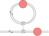
$${\langle{\cal O}_{20^{\prime}}\rangle\hskip-30.0pt} {=} {=} {\mp} {{}+\ldots} {{1\over p^{2}+m_{ab}^{2}}} {=} {{}\ {1\over p^{2}+m_{(0)ab}^{2}}} {\mp} {{\lambda\langle{\cal O}_{20^{\prime}}\rangle\over(p^{2}+m_{(0)ab}^{2})(p^{2}+m_{ab}^{2})}} {{}+\ldots} {\hfill m_{ab}^{2}} {=} {{}m_{(0)ab}^{2}\pm\lambda\langle{\cal O}_{20^{\prime}}\rangle+\ldots\hfill}$$      

Figure 2: Self-consistent treatment of leading order color-independent corrections to masses of the scalar $X_{i}$. The shaded circle indicates the full dressed propagator, and $a$ and $b$ are color indices. The operator $({\cal O}_{20^{\prime}})^{2}$ is represented as a dotted line connecting the two ${\cal O}_{20^{\prime}}$ insertions. The $\pm$ sign is chosen according as ${\cal O}_{20^{\prime}}$ includes a positive or negative mass term for $X_{i}$.

References

- [1] J. Maldacena, “The Large N limit of superconformal field theories and supergravity,” Adv. Theor. Math. Phys. 2 (1998) 231, hep-th/9711200.
- [2] S. S. Gubser, I. R. Klebanov, and A. M. Polyakov, “Gauge theory correlators from noncritical string theory,” Phys. Lett. B428 (1998) 105, hep-th/9802109.
- [3] E. Witten, “Anti-de Sitter space and holography,” Adv. Theor. Math. Phys. 2 (1998) 253, hep-th/9802150.
- [4] J. A. Minahan and N. P. Warner, “Quark potentials in the Higgs phase of large N supersymmetric Yang-Mills theories,” JHEP 06 (1998) 005, hep-th/9805104.
- [5] I. R. Klebanov and E. Witten, “AdS / CFT correspondence and symmetry breaking,” hep-th/9905104.
- [6] D. Z. Freedman, S. S. Gubser, K. Pilch, and N. P. Warner, “Renormalization group flows from holography—supersymmetry and a c-theorem,” hep-th/9904017.
- [7] B. de Wit and H. Nicolai, “The consistency of the truncation in supergravity,” Nucl. Phys. B281 (1987) 211.
- [8] H. Nastase, D. Vaman, and P. van Nieuwenhuizen, “Consistent nonlinear K K reduction of 11-d supergravity on AdS(7) x S(4) and selfduality in odd dimensions,” hep-th/9905075.
- [9] M. Gunaydin, L. J. Romans, and N. P. Warner, “Gauged supergravity in five-dimensions,” Phys. Lett. 154B (1985) 268.
- [10] M. Pernici, K. Pilch, and P. van Nieuwenhuizen, “Gauged N=8 D=5 supergravity,” Nucl. Phys. B259 (1985) 460.
- [11] M. Gunaydin, L. J. Romans, and N. P. Warner, “Compact and noncompact gauged supergravity theories in five-dimensions,” Nucl. Phys. B272 (1986) 598.
- [12] A. Khavaev, K. Pilch, and N. P. Warner, “New vacua of gauged N=8 supergravity in five-dimensions,” hep-th/9812035.
- [13] J. Distler and F. Zamora, “Nonsupersymmetric conformal field theories from stable anti-de Sitter spaces,” hep-th/9810206.
- [14] P. Kraus, F. Larsen, and S. P. Trivedi, “The Coulomb branch of gauge theory from rotating branes,” JHEP 03 (1999) 003, hep-th/9811120.
- [15] A. Chamblin, R. Emparan, C. V. Johnson, and R. C. Myers, “Charged AdS black holes and catastrophic holography,” hep-th/9902170.
- [16] M. Cvetic and S. S. Gubser, “Phases of R charged black holes, spinning branes and strongly coupled gauge theories,” hep-th/9902195.
- [17] M. Cvetic et. al., “Embedding AdS black holes in ten-dimensions and eleven-dimensions,” hep-th/9903214.
- [18] K. Behrndt, M. Cvetic, and W. Sabra, “Nonextreme black holes of five-dimensional N=2 AdS supergravity,” hep-th/9810227.
- [19] A. Kehagias and K. Sfetsos, “On asymptotic freedom and confinement from type IIB supergravity,” hep-th/9903109.
- [20] J. A. Minahan, “Asymptotic freedom and confinement from type 0 string theory,” hep-th/9902074.
- [21] S. S. Gubser, “Dilaton driven confinement,” hep-th/9902155.
- [22] L. Girardello, M. Petrini, M. Porrati, and A. Zaffaroni, “Confinement and condensates without fine tuning in supergravity duals of gauge theories,” hep-th/9903026.
- [23] C. Csaki, Y. Oz, J. Russo, and J. Terning, “Large N QCD from rotating branes,” Phys. Rev. D59 (1999) 065012, hep-th/9810186.
- [24] M. Cvetic and S. S. Gubser, “Thermodynamic stability and phases of general spinning branes,” hep-th/9903132.
- [25] I. R. Klebanov, “World volume approach to absorption by nondilatonic branes,” Nucl. Phys. B496 (1997) 231, hep-th/9702076.
- [26] D. Anselmi, D. Z. Freedman, M. T. Grisaru, and A. A. Johansen, “Nonperturbative formulas for central functions of supersymmetric gauge theories,” Nucl. Phys. B526 (1998) 543, hep-th/9708042.
- [27] D. Anselmi, J. Erlich, D. Z. Freedman, and A. A. Johansen, “Positivity constraints on anomalies in supersymmetric gauge theories,” Phys. Rev. D57 (1998) 7570–7588, hep-th/9711035.
- [28] S. S. Gubser and I. R. Klebanov, “Absorption by branes and Schwinger terms in the world volume theory,” Phys. Lett. B413 (1997) 41–48, hep-th/9708005.
- [29] P. S. Howe, E. Sokatchev, and P. C. West, “Three point functions in N=4 Yang-Mills,” Phys. Lett. B444 (1998) 341, hep-th/9808162.
- [30] A. Petkou and K. Skenderis, “A Nonrenormalization theorem for conformal anomalies,” hep-th/9906030.
- [31] S.-J. Rey and J. Yee, “Macroscopic strings as heavy quarks in large N gauge theory and anti-de Sitter supergravity,” hep-th/9803001.
- [32] J. Maldacena, “Wilson loops in large N field theories,” Phys. Rev. Lett. 80 (1998) 4859, hep-th/9803002.
- [33] A. W. Peet and J. Polchinski, “UV / IR relations in AdS dynamics,” Phys. Rev. D59 (1999) 065011, hep-th/9809022.
- [34] G. T. Horowitz and J. Polchinski, “A Correspondence principle for black holes and strings,” Phys. Rev. D55 (1997) 6189–6197, hep-th/9612146.
- [35] D. Kabat, talk on joint work with G. Lifschytz at “Black Holes II,” Montreal, June 1999.
- [36] A. Brandhuber and K. Sfetsos, “Wilson loops from multicentre and rotating branes, mass gaps and phase structure in gauge theories,” hep-th/9906201.