A Note on Classical String Dynamics on AdS₃

Abstract

We consider bosonic strings propagating on Euclidean adS₃, and study in particular the realization of various worldsheet symmetries. We give a proper definition for the Brown-Henneaux asymptotic target space symmetry, when acting on the string action, and derive the Giveon-Kutasov-Seiberg worldsheet contour integral representation simply by using Noether’s theorem. We show that making identifications in the target space is equivalent to the insertion of an (exponentiated) graviton vertex operator carrying the corresponding charge. Finally, we point out an interesting relation between 3D gravity and the dynamics of the worldsheet on adS₃. Both theories are described by an $SL(2,$C$)/SU(2)$ WZW model, and we prove that the reduction conditions determined on one hand by worldsheet diffeomorphism invariance, and on the other by the Brown-Henneaux boundary conditions, are the same.

I Introduction

Classical three-dimensional gravity was shown by Brown and Henneaux [1] to admit an infinite-dimensional conformal symmetry acting on the space of solutions which are asymptotic to anti-de Sitter space (adS₃). An important feature of this symmetry is that the central extension, with charge

$$c_{0} = \frac{3l}{2G_{3}},$$ (1)

where $l$ is the adS₃ scale, and $G_{3}$ is the three-dimensional Newton constant, arises through the necessity for boundary conditions at infinity, and not through normal ordering as conventionally occurs quantum mechanically in two dimensional conformal field theories (CFTs). The manner in which this symmetry is realized has recently come under scrutiny after it was pointed out by Strominger [2] that a CFT at the boundary, forming a unitary representation of the Brown-Henneaux symmetry, would have a density of states sufficiently large to account for the Bekenstein-Hawking entropy of three-dimensional BTZ black holes [3, 4]. In this regard, the essentially classical origin of the central charge has presented an additional challenge for understanding the corresponding microstates.

More generally, the adS/CFT correspondence [5, 6] implies in this instance a duality between string theory on adS₃ (times some compact space) and a two dimensional CFT. In a suitable limit, the correspondence reduces to one between supergravity on this space, and a limit of the CFT in which it should realize the Brown-Henneaux Virasoro symmetry, with its semi-classical central charge. It is then clearly of interest to study string dynamics on adS₃, in the hope of understanding the microscopic origin of (1), and possible quantum corrections to it and the corresponding black hole entropy.

One is generally hampered in studying aspects of the adS/CFT correspondence beyond the supergravity approximation, as the relevant backgrounds necessarily involve nonzero Ramond-Ramond (RR) sector fields, for which the worldsheet description is poorly understood (although see [7] for recent work). However, adS₃ is the fortunate exception here in that there is a well-defined 10-dimensional string background, corresponding to a configuration of fundamental strings and wrapped NS5 branes, for which all the RR fields may be set to zero and a conventional worldsheet description is possible. Indeed, string theory on adS₃ itself has a long history, initiated in [8], as it provides a useful testing ground for quantum consistency (see e.g. [9]). Within the context of the NS1/NS5 system, and the adS/CFT correspondence, the relevant background is adS${}_{3}\times S^{3}\times M^{4}$ (where $M^{4}$ is either $T^{4}$ or K3), and worldsheet aspects of this system were studied initially by Giveon, Kutasov and Seiberg [10], and have since been investigated in [11, 12, 13, 14, 15, 16]. One outcome of this work has been the realization, clarified in [13, 12], that string theory on adS₃ has, in particular, a sector of “long strings”(see also [17]) in which the worldsheet wraps around the boundary of the target space and is effectively non-compact. This sector is governed by an effective Liouville system [13], and its S-dual formulation in the D1/D5 system was identified in [13] with the small instanton singularity in the moduli space of the worldvolume gauge theory. This latter sector is of particular interest since the worldsheet lives in the asymptotic region of the target space, and thus should admit Brown-Henneaux diffeomorphisms as a symmetry. The main purpose of this note is to study the symmetries associated with worldsheet dynamics on adS₃ and clarify, in particular, the realization of the Brown-Henneaux target space symmetry. Following the initial work of [10], this aspect was further elucidated in the work of de Boer et al. [11] who emphasized the distinction between the symmetry of the first quantized string Hilbert space discussed in [10], and the graviton vertex operators associated with Brown-Henneaux diffeomorphisms of the target space. In this paper, we shall make the relation between these two symmetries more explicit in several ways, and emphasize how the classical origin of (1) in pure gravity is mirrored in string theory.

In particular, we find that the spacetime Virasoro operators of [10] may be obtained directly via a classical Noether construction associated with the asymptotic symmetry of the worldsheet action under Brown-Henneaux diffeomorphisms. The charges are conserved asymptotically in the target space and thus this symmetry applies rather naturally to the long string sector. We also find that, as in the gravity description, the central extension (1) is visible within classical Poisson brackets.

A related issue concerns strings propagating on backgrounds which differ topologically from adS₃. Solutions to classical 3D gravity with negative cosmological constant, or equivalently the low energy equations of motion of the string, are all locally isomorphic to adS₃, and differ only in their global structure. Starting from adS₃ one may construct these backgrounds via the process of identifying along discrete symmetries. Since the worldsheet action inherits the symmetries of the target space, one can make use of an analogous procedure to obtain strings propagating on more general backgrounds. Specifically, we shall show that identifying along discrete symmetries of the worldsheet action changes the topology of the target space, naturally leading to the identification of the vertex operators associated with BTZ black holes and conical singularities.

Several interesting features emerge from the analysis of these symmetries. In particular, we find that the reduction conditions for the 3D Einstein-Hilbert action associated with the Brown-Henneaux boundary conditions, shown in [18] to lead to an asymptotic Liouville dynamics, are actually equivalent to the constraints imposed by diffeomorphism invariance on the string worldsheet. As a consequence, we are able to associate the asymptotic dynamics of 3D gravity, with a constrained worldsheet action for a bosonic string propagating on $H^{+}_{3}=SL(2,$C$)/SU(2)$.

The plan of the paper is as follows. In Section II we discuss in some detail the symmetries of the worldsheet action defined on adS₃. In particular, we distinguish between the affine worldsheet symmetry descending from its definition as a coset WZW model, and the asymptotic target space symmetry associated with Brown-Henneaux diffeomorphisms. In the latter case, we define an asymptotic Noether charge in the usual manner, which is shown to be equivalent to the spacetime generators of [10]. In Section III we show how, on identifying along discrete symmetries, one induces vertex operators which on exponentiation change the topology of the target space, leading for example to black hole geometries. In Sec. IV we consider the required gauge fixing conditions for the worldsheet dynamics, and show that the resulting dynamics is that of Liouville theory, and that in the long string sector the spacetime generator is directly related to the generator of conformal transformations on the worldsheet. In Section V, we explore the relation between the gauge fixed worldsheet dynamics and the usual reduction of 3D gravity to Liouville theory, via the use of an auxiliary manifold, whose boundary we identify with the string worldsheet. We conclude in Section 5 with some additional remarks on the issue of black hole microstates.

II Classical dynamics of strings on adS₃.

An important property of the Brown-Henneaux conformal symmetry [1], discussed earlier, is that the central charge is related, not to normal ordering ambiguities, but to boundary conditions. For this reason it is visible classically. This is also the case in the string theoretic description of this symmetry, at least in the so-called “long string” sector in which the string wraps around the adS₃ boundary. In this section, we study the classical dynamics of a string propagating on adS₃. We shall give in Sec. II B a proper definition of the Brown-Henneaux symmetry acting on the string, and derive the contour integral representation for the generators proposed in [10], as classical Noether charges.

A The action and worldsheet symmetries

The worldsheet theory for bosonic strings propagating on the coset manifold $H^{+}_{3}=SL(2,$C$)/SU(2)$ (or Euclidean adS₃) is described by an $SL(2,$C$)$ WZW action,

$$I_{W}[h] = -\frac{k}{2\pi}\int_{\Sigma}{\rm tr}(h^{-1}\partial h)(h^{-1}\overline{\partial}h)+\frac{ik}{12\pi}\int_{\Sigma}d^{-1}{\rm tr}(h^{-1}dh)^{3},$$ (2)

where $k$ is the WZW level, which throughout we shall take to be large, and the group element $h$ is restricted to lie in the above coset, the space of $2\times 2$ hermitian complex matrices with unit determinant. This model has two affine $SL(2,$C$)$ symmetries, which are identified under complex conjugation. The generators for these symmetries are the currents, $J=h^{-1}\partial h$ and its conjugate $\overline{J}$.

If we parametrise the coset with coordinates $(\phi,\gamma,\overline{\gamma})$,

$$h = \left(\begin{array}[]{cc}e^{-\phi}+\gamma\overline{\gamma}e^{\phi}&e^{\phi}\gamma\\ e^{\phi}\overline{\gamma}&e^{\phi}\end{array}\right),$$ (5)

then the action for the string worldsheet takes the following form

$$I_{W}[\phi,\gamma,\bar{\gamma}]={k\over 2\pi i}\int_{W}(\partial\phi\bar{\partial}\phi+e^{2\phi}\partial\bar{\gamma}\bar{\partial}\gamma)d^{2}z.$$ (6)

For later convenience, the volume element is taken to be $d^{2}z=dz\mbox{$\wedge$}d\bar{z}$, and the factor $i$ in the coefficient then ensures that the action is real. Recently, (6) has been the object of intense study due to its important relation with the adS/CFT correspondence [10, 11, 12, 13, 14, 15, 16]. Our aim here is to describe some aspects of this action which may help to understand its spacetime conformal properties.

The affine currents above can be decomposed into an $SL(2,$C$)$ basis as $J=J^{a}T_{a}=kh^{-1}\partial h/2$, which in the parametrization (5), and with a convenient rescaling $\phi\rightarrow\phi/\sqrt{2k}$, $\gamma\rightarrow\gamma/\sqrt{k}$ and $\bar{\gamma}\rightarrow\bar{\gamma}/\sqrt{k}$, take the form,

$$J^{-} = \beta$$ (7)

$$J^{3} = \beta\gamma+{\alpha\over 2}\partial\phi$$ (8)

$$J^{+} = \beta\gamma^{2}+\alpha\,\gamma\partial\phi+k\partial\gamma,$$ (9)

where we have introduced $\beta=-e^{2\phi/\alpha}\partial\overline{\gamma}$ and $\alpha=\sqrt{2k}$. One recognizes these currents as those arising from the free field representation of the affine current algebra [19], in which $\beta$ is treated dynamically. The corresponding action takes the form,

$$I[\phi,\gamma,\bar{\gamma},\beta,\bar{\beta}]={1\over 2\pi i}\int\left({1\over 2}\partial\phi\bar{\partial}\phi-\beta\bar{\partial}\gamma-\bar{\beta}\partial\bar{\gamma}-e^{-2\phi/\alpha}\beta\bar{\beta}\right)d^{2}z.$$ (10)

Varying this action with respect to $\beta$ and $\bar{\beta}$ one obtains (6) in terms of the rescaled fields. Note that since we take $k$ large, we work classically and ignore quantum corrections $\alpha\rightarrow\sqrt{2(k-2)}$ affecting the screening charge, and an induced linear dilaton coupling. For a discussion of related quantum effects see Refs. [8, 9, 10, 12].

In the large $\phi$ sector the last term in (10) is a perturbation and one can use the free OPE representation,

$$\phi(z)\phi(z^{\prime})\sim-\log(z-z^{\prime}),\ \ \ \ \ \ \beta(z)\gamma(z^{\prime})\sim{1\over z-z^{\prime}}.$$ (11)

Note that the rescaling of $\phi$ is such that its kinetic term appears divided by two in (10). This factor is necessary in order to obtain the OPE (11) which then leads to the $SL(2,C)$ algebra at level $k$ for the affine currents defined above. These currents are holomorphically conserved, $\bar{\partial}J^{a}=0$, as may be checked by using the equations of motion following from (10).

As a consequence of its affine symmetry, the action (6) has a worldsheet conformal symmetry, corresponding to mappings $z\rightarrow f(z)$, with central charge $c=3k/(k-2)\sim 3$. The stress tensor which generates the corresponding Virasoro algebra takes the Sugawara form, $T_{W}=(J^{+}J^{-}-(J^{3})^{2})/k$, and is (classically)

$$T_{W}=\beta\partial\gamma-{1\over 2}(\partial\phi)^{2}.$$ (12)

Quantum mechanically, normal ordering generates an improvement term for $\phi$ which is subleading in $k$ and generates the central charge $c\sim 3$.

The dynamics of the string worldsheet is given by the equations of motion, varying with respect to the fields, plus the equation,

$$T_{W}=0,$$ (13)

and its conjugate $\bar{T}_{W}=0$, which are required in order to ensure worldsheet diffeomorphism invariance. Since we focus on classical aspects of the dynamics we have, in writing this constraint, ignored the presence of a product manifold ($M$) in the string background (adS${}_{3}\times M$), and also additional matter fields. While these will be required quantum mechanically to ensure vanishing of the total central charge, they will not affect our discussion, and we shall now focus on the adS₃ sector.

As we have stressed above, most of the aspects of the Brown-Henneaux symmetry are visible classically, and thus we could also work at the level of Poisson brackets. A useful representation for the symplectic structure, motivated by the above OPE’s, follows by using a (holomorphic) “lightcone” decomposition. We shall treat $\bar{z}$ as the time coordinate. In this situation, the fields $\bar{\beta}$ and $\bar{\gamma}$ become “Lagrange multipliers” because they enter in the action (10) without “time” derivatives. On the other hand, the fields $\beta$ and $\gamma$ are canonically conjugate and we derive the “equal-time” Poisson bracket,

$$[\beta(z),\gamma(z^{\prime})]=\delta(z,z^{\prime}).$$ (14)

We define the Dirac delta function as $\oint(dz/2\pi i)f(z^{\prime})\delta(z,z^{\prime})=f(z)$.

The field $\phi$ also appears in the action with a linear time derivative. In order to extract the Poisson bracket of $\phi$ with itself we need to assume that the operator $\partial$ is invertible. The invertibility of $\partial$ is achieved by fixing the value of $\phi$ at infinity $\phi(z\rightarrow\infty)\rightarrow\phi_{\infty}$. An explicit inverse for this operator can be written as $\partial^{-1}f(z)=\oint(dz/2\pi i)f(z^{\prime})\theta(z,z^{\prime})$ where $\theta(z,z^{\prime})$ is the step function satisfying $\partial\theta(z,z^{\prime})=\delta(z,z^{\prime})$. The equal time Poisson bracket for $\phi(z)$ is then,

$$[\phi(z),\phi(z^{\prime})]=-\theta(z,z^{\prime}).$$ (15)

The similarity between the OPE’s (11) and the Poisson brackets (14) and (15) should be evident.

The Hamiltonian density for this system can be read off directly from (10). Integrating over a “spatial slice” yields,

$$H=\oint{dz\over 2\pi i}\,e^{-2\phi/\alpha}\beta\bar{\beta}.$$ (16)

(The term $\bar{\beta}\partial\bar{\gamma}$ has zero Poisson bracket with all fields so we omit it.) It is a straightforward exercise to find the Hamilton equations,

$$\bar{\partial}\beta = [\beta(z),H]=0$$ (17)

$$\bar{\partial}\gamma = [\gamma(z),H]=-e^{-2\phi/\alpha}\bar{\beta}$$ (18)

$$\bar{\partial}\phi = [\phi(z),H]={2\over\alpha}\oint{dz^{\prime}\over 2\pi i}(e^{-2\phi/\alpha}\beta\bar{\beta})(z^{\prime})\theta(z,z^{\prime}).$$ (19)

The first two relations are of course the equations of motion which follow from varying (10) with respect to $\gamma$ and $\beta$. The third equation can be put in a more familiar form by applying the (invertible) operator $\partial$ to both sides (using $\partial\theta(z,z^{\prime})=\delta(z,z^{\prime})$) obtaining,

$$\partial\bar{\partial}\phi={2\over\alpha}\,e^{-2\phi/\alpha}\beta\bar{\beta},$$ (20)

which is the correct equation of motion for $\phi$. The Hamiltonian (16) plus the canonical relations (14) and (15) represent a (holomorphic) canonical version of the action (10).

The conservation of the currents, $\bar{\partial}J^{a}=0$, may also be expressed in Hamiltonian form as,

$$[J^{a}(z),H]=0,$$ (21)

which can be proved directly from the above formulae for $J^{a}(z)$, $H$, and the Poisson brackets. In the same way, one may check that the currents $J^{a}$ satisfy the $SL(2,C)$ algebra at level $k$, and that the worldsheet stress-tensor $T_{W}$ defined in (12) satisfies the expected classical algebra,

$$[T_{W}(z),T_{W}(z^{\prime})]=-(T_{W}(z)+T_{W}(z^{\prime}))\partial\delta(z,z^{\prime}),$$ (22)

generating holomorphic worldsheet conformal transformations. Quantum mechanically, (22) develops a central charge $c\sim 3$, as mentioned above.

Thus far we have focussed on the conventional worldsheet symmetry of the action (6). However, since (6) describes a string propagating on adS₃, one also expects a realization of the Brown-Henneaux [1] spacetime conformal symmetry, corresponding to mappings $\gamma\rightarrow f(\gamma)$, with a classical central charge $c\sim 6k$. We shall now analyze this symmetry in detail.

B The Brown-Henneaux spacetime conformal symmetry

In conformal gauge, the action for a string propagating on a curved background with metric $G_{\mu\nu}$ and antisymmetric tensor field $B_{\mu\nu}$ takes the usual sigma model form,

$$I[X]=\frac{k}{4\pi i}\int_{W}d^{2}z\left(G_{\mu\nu}(X)\delta^{ab}\partial X^{\mu}_{a}\bar{\partial}X^{\nu}_{b}+iB_{\mu\nu}(X)\epsilon^{ab}\partial X^{\mu}_{a}\bar{\partial}X^{\nu}_{b}\right).$$ (23)

The spacetime symmetries of this action are given by the Killing vectors of the spacetime metric $G_{\mu\nu}$ and antisymmetric tensor $B_{\mu\nu}$. In the simplest case, the target metric is flat, $G_{\mu\nu}=\eta_{\mu\nu}$, and the action is Poincaré invariant.

If we now denote $X^{\mu}=(\phi,\gamma,\bar{\gamma})$, and revert momentarily to the “geometric field normalization” of (6), the metric $G$ and field $B$ associated with the action (6) are

$$ds^{2} = d\phi^{2}+e^{2\phi}d\gamma d\bar{\gamma},$$ (24)

$$B = e^{2\phi}d\gamma\mbox{$\wedge$}d\bar{\gamma}.$$ (25)

The metric (24) is a maximally symmetric line element having 6 Killing vectors. These isometries lead to the six dimensional affine symmetry of the worldsheet action generated by the currents (8) and their conjugates.

As pointed out long ago by Brown and Henneaux [1], the line element (24) has another interesting asymptotic ($\phi\rightarrow\infty$) symmetry given by the transformations,

$$\delta_{\mbox{{BH}}}\gamma = -\varepsilon(\gamma)$$ (26)

$$\delta_{\mbox{{BH}}}\bar{\gamma} = \frac{1}{2}\,e^{-2\phi}\varepsilon^{\prime\prime}(\gamma)$$ (27)

$$\delta_{\mbox{{BH}}}\phi = \frac{1}{2}\,\varepsilon^{\prime}(\gamma)$$ (28)

where $\varepsilon(\gamma)$ is an arbitrary function of $\gamma$, and $\varepsilon^{\prime}$ denotes the derivative with respect to $\gamma$. Acting with these transformations on (24) and (25) one generates a new background,

$$ds^{2}_{new} = d\phi^{2}+e^{2\phi}d\gamma d\bar{\gamma}+\frac{1}{2}\varepsilon^{\prime\prime\prime}d\gamma^{2}$$ (29)

$$B_{new} = e^{2\phi}d\gamma\mbox{$\wedge$}d\bar{\gamma}+\varepsilon^{\prime\prime}d\phi\mbox{$\wedge$}d\gamma.$$ (30)

The correction for $B$ is clearly a gauge transformation because $\varepsilon$ depends only on $\gamma$ ($dB_{new}=dB)$. On the other hand, the correction for the metric is subleading in $\phi$. This is why the Brown-Henneaux transformations only leave the anti-de Sitter metric invariant asymptotically.

Before applying this symmetry to the worldsheet action we pause to mention an important aspect of the Brown-Henneaux transformations (27). Two metrics which differ by a transformation of the form (27) are physically distinguishable because the canonical generator implementing the transformation is a non-zero quantity, the Virasoro charge [1]. Since in three dimensions there are no gravitational waves, it follows that all solutions to the equations of motion can be generated from anti-de Sitter space via a finite Brown-Henneaux transformation. One can then write the general solution to the equations of motion with anti-de Sitter boundary conditions in the form,

$$ds^{2}=d\phi^{2}+e^{2\phi}d\gamma d\bar{\gamma}-{6T(\gamma)\over c}d\gamma^{2}$$ (31)

where $T(\gamma)$ is an arbitrary function of $\gamma$. (One can also include an arbitrary function of $\bar{\gamma}$, but for simplicity in this paper we will restrict all discussions to the holomorphic sector.) The anti-de Sitter metric corresponds to the vacuum state with $T=0$ which is $SL(2,C)$ invariant. Acting with the infinitesimal Brown-Henneaux transformations one generates a non-zero $T_{new}=-(c/12)\varepsilon^{\prime\prime\prime}$, as in (29). The line element (31) will appear repeatedly in our analysis. See [2, 20, 21] for recent discussions.

We now return to the worldsheet action, and consider how the transformations (27), which generate asymptotic symmetries of the background fields (24) and (25), are manifested as symmetries of the action. For this to be the case, it is necessary to consider strings whose worldsheet is embedded in the region near the boundary of adS₃, i.e. $\phi\rightarrow\infty$. The action (6) is then invariant under the transformations (27) up to boundary terms.

In order to make contact with the currents (8) and the operator found in [10], we shall work with the action (10) instead of (6). The Brown-Henneaux transformations (27) are easily translated to the holomorphic sector $\{\phi,\gamma,\beta\}$. The leading terms are,

$$\delta_{\mbox{{BH}}}\gamma = -\varepsilon,$$ (32)

$$\delta_{\mbox{{BH}}}\beta = \varepsilon^{\prime}\beta+{\alpha\over 2}\,\varepsilon^{\prime\prime}\partial\phi,$$ (33)

$$\delta_{\mbox{{BH}}}\phi = {\alpha\over 2}\,\varepsilon^{\prime}.$$ (34)

We also note that, under holomorphic transformations, $\delta_{\mbox{{BH}}}\overline{\beta}=0$. An important property of these diffeomorphisms is that they leave invariant the worldsheet stress-tensor,

$$\delta_{\mbox{{BH}}}T_{W}=0,$$ (35)

where $T_{W}$ is defined in (12). Since $T_{W}$ is constrained by diffeomorphism invariance to be zero, this equation reflects an important consistency condition. If the product manifold $M$ is added and $T_{W}=0$ is replaced by $T_{W}+T_{M}=0$, this equation means that the Brown-Henneaux diffeomorphisms do not mix $T_{W}$ and $T_{M}$.

We shall now prove that the action (10) is invariant, up to boundary terms, under (33). For illustration it will be convenient to take a canonical perspective and view the worldsheet as interpolating between specified initial and final closed string configurations. At tree level, a worldsheet without any additional sources then has a cylindrical topology, and may be mapped to an annulus within the usual prescription for radial quantization. In this formulation, one finds that total derivative terms arising from variations of the worldsheet action reduce to contour integrals at the initial and final boundaries. Thus the variation of the action (10) under a Brown-Henneaux diffeomorphism (33) is,

$$\delta_{\mbox{{BH}}}I=-{\alpha\over 4}\sum_{j}\left(\oint_{C_{j}}{d\bar{z}\over 2\pi i}\,\varepsilon^{\prime}\bar{\partial}\phi+\oint_{C_{j}}{dz\over 2\pi i}\,\varepsilon^{\prime}\partial\phi\right)$$ (36)

in which the contours ${C_{j}}$ surround the worldsheet boundaries, and we have discarded a subleading term in $\phi$. (In the derivation of (36) we have used $\int d^{2}z\bar{\partial}F=\oint dzF$ and $\int d^{2}z\partial F=-\oint d\bar{z}F$.)

Via the state–operator map we can always replace the boundary configurations with operator insertions leading to the conventional spherical topology with insertions at the boundary points. However, we shall find that the original canonical picture is more helpful in the next subsection where we shall consider the Noether charge for this asymptotic symmetry.

Before turning to this discussion we point out that the above analysis naturally encompasses the short and long string sectors of the theory. In the long string sector, where the worldsheet wraps the entire boundary at conformal infinity ($\phi\rightarrow\infty$) in adS₃, the annulus description for the worldsheet extends to the full complex plane, and contour integrals surround infinity. In the short string sector the worldsheet does not wrap the boundary, and may for example be associated with a correlator of a set of vertex operators inserted at points $\{z_{i}\}$ on the worldsheet. As shown in [11], the worldsheet then develops thin tubes out to conformal infinity, $\phi\rightarrow\infty$, at each insertion point. It is clear that in this case, there are additional boundaries for the worldsheet associated with regularization near each insertion point. Each insertion point will then lead to an additional contour integral in (36).

C The Noether charge

Since the variation of (10) under Brown-Henneaux transformations (33) reduces to a boundary term, there is a Noether charge associated with this symmetry. As usual, the charge is the canonical generator of (33). In this section we shall explicitly compute this charge, which we find to be equal to the Giveon-Kutasov-Seiberg operator [10].

Consider a single closed string in an initial state 1, with coordinates $\{\gamma_{1}(z),\bar{\gamma}_{1}(z),\phi_{1}(z)\}$, and a final state 2 with coordinates $\{\gamma_{2}(z),\bar{\gamma}_{2}(z),\phi_{2}(z)\}$. (Our arguments will generalize trivially to a more general solution.) We assume that both $\phi_{1}$ and $\phi_{2}$ are large. The worldsheet connects the initial and final configurations generating a cylinder (or some other higher genus surface) parametrised by the “time” coordinate $\bar{z}$ (see Fig. 1). As mentioned earlier, a key assumption we shall need to make is that the initial and final conditions are such that the full classical worldsheet is contained in the large $\phi$ region. This assumption will not be fulfilled in general but it is valid, for example, in the long string sector [12, 13].

Due to the Brown-Henneaux symmetry of the large $\phi$ sector, there is a conserved charge associated with the above diagram. A quick derivation of the Noether charge follows by comparing (36) with the on-shell variation of the action.

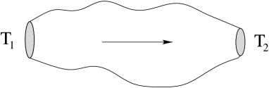
FIG. 1.: A schematic representation of a classical (large $\phi$) worldsheet configuration interpolating two boundary configurations. Under a Brown-Henneaux target space diffeomorphism, one generates “charges” $T_{i}$ at the boundaries, and the asymptotic symmetry ensures the conservation condition $T_{1}=T_{2}$ within this diagram.

A generic (holomorphic) variation of the action (10) reads,

$$\delta I=(eom)+{1\over 2}\sum_{j}\left(\oint_{C_{j}}{dz\over 2\pi i}\,\delta\phi\partial\phi-\oint_{C_{j}}{d\bar{z}\over 2\pi i}\,\delta\phi\bar{\partial}\phi-2\oint_{C_{j}}{dz\over 2\pi i}\,\beta\delta\gamma\right)$$ (37)

where $(eom)$ represents the equations of motion. As before, the contour integrals are defined at the worldsheet boundaries. In the situation shown in Fig. 1, the boundaries correspond to the initial and final configurations and $j=1,2$. The string is closed and for simplicity we assume that there are no additional insertions, although as mentioned earlier the initial and final configurations could be replaced via the state-operator map with two insertions. We now substitute in this expression the variations (33), set the term $(eom)$ to zero, and compare the result with (36). We find that the contour integrals $\oint d\bar{z}$ cancel out. The Noether identity contains only holomorphic contours and reads,

$$\sum_{i}T^{i}_{\varepsilon}=0, \;\;\;\;\;\;\;T^{i}_{\varepsilon}=-\oint_{i}{dz\over 2\pi i}\left({\alpha\over 2}\varepsilon^{\prime}\partial\phi+\varepsilon\beta\right).$$ (38)

This relation expresses the on-shell conservation of the “charge” $T^{i}_{\varepsilon}$. In the simplest situation with only two boundaries at the states 1 and 2, the above equation reads $T^{1}_{\varepsilon}=T^{2}_{\varepsilon}$ (taking the orientation into account) which explicitly states the conservation of $T_{\varepsilon}$.

The conservation equation can also be derived by the usual trick of letting $\varepsilon$ be a function of $\bar{z}$, that is, $\varepsilon=\varepsilon(\gamma,\bar{z})$ . Varing the action with this coordinate-dependent parameter, one finds $\bar{\partial}t_{\varepsilon}=0$ with $t_{\varepsilon}=(\alpha/2)\varepsilon^{\prime}\partial\phi+\varepsilon\beta$.

As is to be expected, the charge $T_{\varepsilon}$ generates the Brown-Henneaux transformations (33) via the Poisson brackets (14) and (15). Indeed, using (14) and (15) it is straightforward to check that $\delta_{\mbox{BH}}\gamma(z)=[\gamma(z),T_{\varepsilon}]$, $\delta_{\mbox{BH}}\phi(z)=[\phi(z),T_{\varepsilon}]$ and $\delta_{\mbox{BH}}\beta(z)=[\beta(z),T_{\varepsilon}]$. The charge $T_{\varepsilon}$ is also a worldsheet conformal invariant,

$$[T_{W},T_{\varepsilon}]=0.$$ (39)

This relation is just the canonical version of (35).

The charges $T_{\varepsilon}$ defined in (38) are infinite in number because $\varepsilon(\gamma)$ is an arbitrary function of $\gamma$. One would like to factor out the parameter $\varepsilon$ and extract the charge as a function of the dynamical variables. However, one notes that the parameter of the transformation $\varepsilon(\gamma)$ is itself a function of a dynamical variable. Let

$$\varepsilon(\gamma)=\sum_{n\in N}\varepsilon^{n}\,\gamma^{n+1},$$ (40)

be a local expansion for $\varepsilon(\gamma)$. Inserting this expansion into the formula for $T_{\varepsilon}$ we find,

$$T_{\varepsilon}=\sum_{n\in N}\varepsilon^{n}\,L_{n},$$ (41)

where we have defined,

$$L_{n} = -\oint{dz\over 2\pi i}\left({\alpha\over 2}(n+1)\gamma^{n}\partial\phi+\gamma^{n+1}\beta\right),$$ (42)

$$= -\oint{dz\over 2\pi i}\left((n+1)\gamma^{n}J^{3}-n\gamma^{n+1}J^{-}\right).$$ (43)

(In the last equality, we have used the formulae for the currents (8).) We recognize the operators $L_{n}$ as the generators deduced in [10]. Note that $L_{n}$ enters correctly in $T_{\varepsilon}$ as the generator of the mode $n$.

The OPE, or commutator of two $L_{n}$’s can be computed easily using (14), (15) and yields the Virasoro algebra with a central charge [10],

$$c=6kp,\ \ \ \ \ \ \ \ p:=\oint{dz\over 2\pi i}{\partial\gamma\over\gamma}.$$ (44)

We stress that this charge arises in both the quantum and classical calculations. If the worldsheet $(\gamma(z,\overline{z}),\overline{\gamma}(z,\overline{z}))$ does not wrap around the adS₃ boundary, as in the short string sector, then $p=0$ and thus the central charge is zero, as was also pointed out in [11]. Or rather it was argued to arise in this sector from disconnected worldsheets, therefore requiring a second quantized description. In this sense, for a single compact worldsheet in the short string sector, the generators (43) do not correspond directly to the Brown-Henneaux operators acting on the supergravity action. We shall make some additional comments on the second quantized description in Section V.

The operators $L_{n}$ first appeared in [10], and were later discussed in [11], where a derivation of (43) similar to ours was presented, and also in [12], although the full interpretation in terms of conserved charges for the asymptotic target space symmetry was not given. Within our construction, since these generators appear as classical Noether charges, it is clear that they can only be used at large $\phi$, where they generate a symmetry of the action. Note that this is a general statement, and not associated with the restricted validity of the free-field representation for large $\phi$.

III Graviton vertex operators and spacetime topology

Anti-de Sitter space is the maximally symmetric solution to the string low energy equations in three dimensions. There exists, however, a continuum of solutions corresponding to changes in the topology as well as propagation of Brown-Henneaux “gravitons” at the boundary. These solutions are well-known from the gravitational point of view, and one may consider a string propagating on these backgrounds [23, 24].

In this section we would like to point out that in complete analogy with the gravitational case, there exists a finite Brown-Henneaux transformation mapping a string propagating on a black hole to a string propagating on adS₃ with an inserted vertex operator. This leads to a natural identification of the black hole vertex operator.

Consider the free string action (6), and let $K$ be a Killing vector of the target adS₃ metric. We will identify points along a discrete subgroup generated by $K$. From the point of view of the target metric, this is just the construction of conical singularities [25] or black holes [4] starting from the anti-de Sitter metric (see [26, 27] for generalizations to other dimensions). The resulting action will be that of a string propagating on a conical singularity, or black hole, depending on the chosen Killing vector $K$. In the black hole case, it is useful to write the metric in coordinates such that $K=\partial_{\theta}$, the identification then takes the “natural” form $\theta\sim\theta+2\pi$, and the metric correspondingly acquires the Schwarzschild form.

We shall now study the consequences of this construction in string theory, explicitly working out the simplest case, corresponding to the generation of an extreme black hole background. In this section, we consider again the “geometrical” action (6). Consider the symmetry of (6) under holomorphic dilatations

$$\gamma\rightarrow\lambda\gamma{\hbox{, \ \ \ \ \ \ \ }}e^{2\phi}\rightarrow e^{2\phi}/\lambda$$ (45)

for a given complex parameter $\lambda$. (Note that $\lambda$ can depend on $z$, although we consider here the simplest situation in which $\lambda$ is constant.) We identify points which differ by the action of the symmetry,

$$\gamma\sim\lambda\gamma,\ \ \ \ \ \ \lambda\in C.$$ (46)

The parameter $\lambda$ is complex and we assume that there exists a number $p$ such that

$$\lambda^{p}=1.$$ (47)

If $p$ is real, this means that $\lambda$ is a root of unity, but we shall not restrict ourselves to this case. Indeed, for real values of $p$ the target metric corresponds to a conical singularity, while for purely imaginary values the identified spacetime has the topology of a solid torus and corresponds to a black hole.

Instead of working with the original fields constrained by the above identifications (as one would do in the orbifold procedure), we make the field redefinitions,

$$\gamma^{\prime} = \gamma^{p},$$ (48)

$$e^{2\phi^{\prime}} = {e^{2\phi}\gamma\over p\gamma^{p}},$$ (49)

$$\bar{\gamma}^{\prime} = \bar{\gamma}+{1-p\over 2e^{2\phi}\gamma},$$ (50)

where $p$ is defined in (47). The key property of the new fields is that the required identifications are now handled automatically because the combinations $\gamma^{p}$ and $e^{2\phi}\gamma$ are invariant under (45). The action for the new fields takes the form (we have erased the primes),

$$I_{p}[\phi,\gamma,\bar{\gamma}]=I[\phi,\gamma,\bar{\gamma}]-\frac{1}{4\pi i}\int d^{2}z\,T(\gamma)\partial\gamma\bar{\partial}\gamma$$ (51)

where $I[\phi,\gamma,\bar{\gamma}]$ is the free action (6) and $T$ is given by

$$T(\gamma)=k{1-p^{-2}\over 2\gamma^{2}},$$ (52)

which as one might expect is proportional to the Schwarzian derivative $\{\gamma^{1/p},\gamma\}$ associated with the map (48). Note that there is also a gauge transformation of the $B$–field, $\delta B=k(p^{-1}-1)/\gamma d\phi\mbox{$\wedge$}d\gamma$, which we shall, however, ignore as it corresponds to a total derivative.

The action (51), resulting from the exponentiation of the induced vertex operator $V_{\gamma\gamma}=T\partial\gamma\bar{\partial}\gamma$, corresponds to a string propagating on the three-dimensional extremal black hole. Indeed, the interaction term in (51) corresponds to adding a piece $T(\gamma)d\gamma^{2}$ to the target space metric, as discussed earlier in Eq. (31). This is not surprising, as the field redefinitions (49) are a particular case of a finite Brown-Henneaux transformation (27). If we take $p=1+\eta$, with $\eta<<1$, the transformation (49) can be put in the form (27) with $\varepsilon(\gamma)=-\eta\gamma\ln\gamma$. Note that in this construction only $L_{0}$ is different from zero. Had we taken $\lambda$ as a function of $z$, which is also a symmetry of the action, we would obtain an action with other Virasoro charges different from zero.

One can also introduce the anti-holomorphic transformation $\bar{\gamma}\rightarrow\bar{\lambda}\bar{\gamma}$ and the solution will no longer be extremal. If $p,\bar{p}$ are real, the identifications induce conical singularities in the target space. If $p,\bar{p}$ are purely imaginary, the target metric is a three-dimensional black hole of mass $M\sim-(p^{-2}+\bar{p}^{-2})$.

IV Gauge Fixing and Liouville Dynamics

In section II, we spent some time considering what happens within the worldsheet theory when one acts on the target space with a Brown-Henneaux diffeomorphism. It is now apparent that there are two symmetries acting on the worldsheet action: the first is the affine symmetry generated by the $SL(2,$C$)$ currents $J\times\overline{J}$; while the second is the conformal symmetry associated with Brown-Henneaux diffeomorphisms which applies asymptotically in the target space.

One can ask whether these symmetries are related, and indeed this is generally true in string worldsheet constructions, in which one obtains spacetime generators by integrating the corresponding worldsheet generators against a suitable vertex operator to ensure the correct conformal dimensions. Within our construction, we have developed the two symmetries separately, and we would now like to see whether they are related in this manner. We shall find that this is indeed the case, once we have imposed the appropriate constraints, and that the resulting dynamics is that of Liouville theory.

A Worldsheet Virasoro Algebra

We begin first with the worldsheet affine algebra generated by the currents (8). The additional constraints that must be imposed are,

$$kT_{W}=J^{+}J^{-}-(J^{3})^{2}=0,\ \ \ \ \ \ \ \ J^{-}=k,$$ (53)

where $J^{a}$ are the currents (8). The first equation expresses diffeomorphism invariance, i.e., the worldsheet stress-tensor is equal to zero (we ignore here any product manifold $M$). The second equation is a gauge fixing condition for the residual conformal symmetry.

It is interesting to invert the roles of $J^{-}=k$ and $T_{W}=0$. Since $J^{-}$ commutes with itself, the equation $J^{-}=k$ can be regarded as a first class constraint with $T_{W}=0$ as the “gauge fixing” condition. It is well-known that the dynamics of the $SL(2,$C$)/SU(2)$ WZW model reduced by $J^{-}=k$, and its conjugate, yields Liouville theory [28, 29]. However, one normally supplements $J^{-}=k$ with a different gauge fixing condition, namely $J^{3}=0$. We shall now prove that imposing $T_{W}=0$ –leaving $J^{3}$ arbitrary– also leads to Liouville theory, and that the current algebra reduces to a Virasoro algebra with central charge $c=6k$.

First, as discussed in [28, 29], it is straightforward to see that the equations of motion following from (10), supplemented by the constraint $J^{-}=k$ and its conjugate, lead directly to Liouville theory. Indeed, the field $\phi$ decouples from $\gamma$ and $\bar{\gamma}$ and satisfies the Liouville equation,

$$\partial\bar{\partial}\phi=\alpha ke^{-2\phi/\alpha}.$$ (54)

The role of the “gauge fixing” constraint is to determine $\gamma$ in terms of $\phi$. In our case, we have imposed $T_{W}=0$ which yields

$$\partial\gamma={1\over 2k}(\partial\phi)^{2}.$$ (55)

(We have already replaced $J^{-}=k$ in this relation.)

The next step, and perhaps the most important, is to show that under the reduction conditions (53), the currents (8) lead to a Virasoro algebra with $c=6k$. In the usual case discussed in the literature, two of the currents, $J^{-}=k$ and $J^{3}=0$, are restricted, while the remaining current $J^{+}$ satisfies the Virasoro with the correct central charge. In our case, the situation is a bit more complicated because the constraint $T_{W}=0$ does not single out a preferred current to play the role of Virasoro operator.

The appropriate operator can be found by first twisting the worldsheet stress tensor $T_{W}$ in such a way that it commutes with the constraint $J^{-}=k$. As discussed in [13] this operator is given by,

$$Q(z):=T_{W}-\partial J^{3}.$$ (56)

Imposing the constaints (53), we find

$$Q(z)=-\partial J^{3}=-{1\over 2}(\partial\phi)^{2}-\sqrt{{k\over 2}}\,\partial^{2}\phi$$ (57)

which we recognize as a stress tensor for the Liouville field $\phi$, and the coefficient of the improvement term implies that $-\partial J^{3}$ generates the Virasoro algebra with $c=6k$ . We shall see in Sec. V a surprising geometrical justification for the appearence of $\partial J^{3}$.

Proceeding a little more carefully, there is actually a technical step in this reduction which should be checked, namely, that the Poisson bracket of $\phi(z)$ with itself is still given by (15), after the gauge is fixed. This turns out to be the case because, after inserting the constraints (53) into the action, the kinetic term for $\phi$ does not change. In the Dirac approach, one constructs the Dirac bracket associated with the second class constraints (53). Using $[\phi(z),J^{-}(z^{\prime})]=0$ one finds $[\phi(z),\phi(z^{\prime})]^{*}=[\phi(z),\phi(z^{\prime})]=-\theta(z,z^{\prime})$ as desired (see the next subsection for more details on the Dirac bracket).

It is instructive to consider this reduction at the level of the action. There is a subtlety here in that the the constraints (53) imply restrictions on derivatives of the fields, and care should be taken to include the appropriate boundary terms to ensure differentiability of the action. However, since this has been discussed in [18], we shall skip the details and write down the gauge fixed form of the action (10),

$$I[\phi]_{gf} = \frac{1}{2\pi i}\int d^{2}z\left(\frac{1}{2}\partial\phi\overline{\partial}\phi-k^{2}e^{-2\phi/\alpha}\right),$$ (58)

which we recognize as the Liouville action in conformal gauge, leading directly to the equation of motion (54). The fields ($\gamma,\overline{\gamma}$) are determined through the constraint $T_{W}=0$ as in (55). Furthermore, if one couples this system to the background worldsheet metric, necessarily with charge $\alpha$ for conformal invariance, one deduces that the stress tensor is given by (57) as expected.

Thus, after imposing the required gauge constraints, one finds that the affine worldsheet symmetry is reduced to a local conformal symmetry with central charge $c=6k$. The dynamics reduces to that of Liouville theory; in particular we have seen that the stress tensor has the Liouville form. This discussion fits quite naturally with the long string discussion in [13], and we note that the reduction is similar to the conventional reduction to Liouville dynamics of 3D gravity. In fact, these two procedures are indeed closely related and we shall make this connection more precise in Section IV. However, we shall now turn to the connection between this Virasoro algebra associated with the gauge fixed worldsheet dynamics, and the Brown-Henneaux asymptotic target space symmetry.

B Worldsheet vs spacetime conformal transformations

The propagation of strings on adS₃ gives rise to two conformal algebras associated with worldsheet transformations $z\rightarrow f(z)$, and spacetime transformations $\gamma\rightarrow F(\gamma)$ for large $\phi$. To summarize the worldsheet discussion of the last subsection, one finds that after the residual conformal freedom is fixed, and the worldsheet stress tensor is set equal to zero, a remnant conformal symmetry survives which may be thought of as a “spectrum generating algebra”. Indeed, the three-dimensional current algebra $J^{a}$ is subject to two conditions (see Eq. (53)). The remaining current, which is conveniently chosen to be $Q=-\partial J^{3}$, was shown to satisfy the Virasoro algebra with $c=6k$. Thus, even after the gauge is fixed we are still left with two Virasoro operators, the Brown-Henneaux generator $T_{\varepsilon}$ defined in (38) (or $L_{n}$ defined in (43)), and the worldsheet generator $Q$.

The operators $L_{n}$ and $Q$ are not in principle related, although they are both constructed in terms of the currents (8). In order to compare $L_{n}$ and $Q$ we need to express $L_{n}$ in terms of the gauge fixed variables. Recall, however, that the charges $L_{n}$ commute with the worldsheet stress tensor and in that sense they are diffeomorphism invariant. This means, in particular, that the algebra of $L_{n}$ does not change after the gauge is fixed.

The gauge-fixed version of $L_{n}$ is obtained by inserting the conditions (53) into the formula (43) for $L_{n}$. This yields,

$$L_{n}[\phi]=-\oint{dz\over 2\pi i}\left({\alpha\over 2}(n+1)\gamma^{n}\partial\phi+k\gamma^{n+1}\right).$$ (59)

We stress here that $\gamma(z)$ should be understood as a functional of $\phi$ determined by (55). The only dynamical variable is $\phi$ whose Poisson (or Dirac) bracket is given by (15). Therefore the gauge-fixed $L_{n}[\phi]$ is a non-local functional (note that $T_{W}=0$ is a differential equation for $\gamma(\phi)$) and generates a complicated transformation for $\phi$. This should not be a surprise since it is well-known that working with gauge fixed variables often yields non-local expressions.

Our task now is to prove that the gauge-fixed $L_{n}[\phi]$ still satisfies the Virasoro algebra with central charge $6kp$ in the Poisson bracket (15). Below we shall give a rigorous proof of this fact. There is, however, an alternative way in which to derive this result which has a nice geometrical interpretation.

After some direct manipulations using the constraints $T_{W}=0$ and $\beta=k$, the functional $L_{n}[\phi]$ can be written conveniently as,

$$L_{n}[\phi]=\oint{dz\over 2\pi i}\,{\gamma^{n+1}\over\partial\gamma}\,Q(z)$$ (60)

where $Q$ is the worldsheet generator given in (57). This formula seems to imply that $L_{n}[\phi]$ is related to $Q$ simply by the transformation $z\rightarrow\gamma(z)$. However, this interpretation is not complete because, on one hand, $\gamma(z)$ is not a function of $z$ but rather a functional of $\phi(z)$, and on the other, the Schwarzian derivative for the map $\gamma(z)$ is not present in (60). Even though $Q$ is a Virasoro density with central charge $6k$, the combination (60) fails to satisfy the Virasoro algebra if the dependence on $\phi$, through $\gamma(\phi)$, is not taken into account.

Nonetheless, in spite of these subtleties, Eq. (60) is an identity and we can use it to relate $L_{n}$ with the modes of $Q$. Let

$$Q(z)=\sum{Q_{n}\over z^{n+2}}$$ (61)

be a local expansion for $Q(z)$. The modes $Q_{n}$ satisfy the Virasoro algebra with $c=6k$. Now consider the sector with $p$ long strings, given by $\gamma(z)=z^{p}+\rho(z)$. The function $\rho(z)$ is a small perturbation of the solution $\gamma=z^{p}$. Replacing the mode decomposition (61) in (60) and keeping only the leading term (independent of $\rho(z)$) we obtain,

$$L_{n}\,=\,\sum_{m}{1\over p}Q_{m}\oint{dz\over 2\pi i}\,{1\over z^{1+m-pn}}\,=\,{1\over p}Q_{pn}$$ (62)

Since $Q_{n}$ is a Virasoro operator with central charge $6k$, this formula implies that $L_{n}$ has central charge $c=6kp$, in full agreement with the results of [10]. The formula (62) has appeared previously in the context of cyclic orbifolds in [30, 31]. In [32, 33] it played a key role in providing a proposal for a statistical mechanical origin for the three-dimensional black hole entropy. We shall come back to this issue in the conclusions.

One point to note is that the transformation (62) maps $Q_{0},Q_{\pm 1}$ into $L_{0},L_{\pm p}$. This implies that the zero mode of $L_{0}$ has to be shifted in order to have $L_{0},L_{\pm 1}$ as generators of the $SL(2,\Re)$ subalgebra. This zero mode shift is equal to the Schwarzian derivative of the map $\gamma=z^{p}$. The absence of this shift in the formula (60) indicates that the analysis above is not complete. In particular, we have only obtained the anticipated algebra with central charge $c=6kp$ for slowly varying perturbations of the solution $\gamma=z^{p}$. Below we shall present a more rigorous discussion and prove that quite generally $L_{n}[\phi]$ indeed satisfies the Virasoro algebra with the correct central charge and zero mode. In fact, the gauge fixed operator $L_{n}[\phi]$ satisfies the same algebra as the original GKS operator $L_{n}$.

This result result follows as a simple consequence of the invariance of $L_{n}$ under the action of $T_{W}$ expressed in the relation $[L_{n},T_{W}]=0$. The necessary tool is the Dirac bracket which has the property that its value does not depend on whether the second class constraints are imposed or not. The Dirac bracket associated to the second class constraints (53) is,

$$[A,B]^{*}=[A,B]+{1\over k}\oint dz\oint dz^{\prime}[A,\beta(z)]\theta(z,z^{\prime})[T_{W}(z^{\prime}),B]$$ (63)

$$+{1\over k}\oint dz\oint dz^{\prime}[A,T_{W}(z)]\theta(z,z^{\prime})[\beta(z^{\prime}),B].$$ (64)

and satisfies $[A,T_{W}(z)]^{*}=0=[A,\beta(z)]^{*}$ for any function $A$. Since $[\beta(z),\phi(z^{\prime})]=0$ we note, in particular, that $[\phi(z),\phi(z^{\prime})]^{*}=[\phi(z),\phi(z^{\prime})]$. Furthermore, $L_{n}[\phi]$ only depends on $\phi$ and thus $[L_{n}[\phi],L_{m}[\phi]]=[L_{n}[\phi],L_{m}[\phi]]^{*}=[L_{n},L_{m}]^{*}$. This last equality is the crucial one; the Dirac bracket of the gauge-fixed $L_{n}[\phi]$ is the same as the Dirac bracket of the original $L_{n}$ before the constraints are imposed. Finally, from $[L_{n},T_{W}]=0$, it is clear that $[L_{n},L_{m}]^{*}=[L_{n},L_{m}]$. The bracket $[L_{n},L_{m}]$ is easy to compute [10] and we find the desired result,

$$[L_{n}[\phi],L_{m}[\phi]]=(n-m)L_{n+m}[\phi]+{c\over 12}n(n^{2}-1)\delta_{n+m,0}$$ (65)

with central charge $c=6kp$.

V String dynamics and three-dimensional gravity

It was pointed out in Section IV that the imposition of constraints such as worldsheet diffeomorphism invariance, naturally reduces the worldsheet affine symmetry to a Virasoro algebra generated by a Liouville stress tensor. It was also pointed out that this reduction has many similarities to the classical Liouville reduction, which appears in 3D gravity[18]. In this section, we shall explore this correspondence, and show that the reduction procedures are indeed equivalent. For this purpose, we shall consider a three-dimensional manifold $M$ whose boundary,

$$W=\partial M,$$ (66)

is to be identified with the string worldsheet (see Fig. 2).

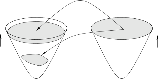
$W=\partial M$

$\phi\rightarrow\infty$                                                                                          $\rho\rightarrow\infty$

Target $:(\phi,\gamma,\overline{\gamma})$                          $M:(\rho,z,\overline{z})$

FIG. 2.: A schematic representation of the embedding of the worldsheet, $W=\partial M$ into the target. The upper embedding, corresponding to “long strings” is the sector which we shall focus on here.

We will show that a gravitational theory on $M$, with anti-de Sitter boundary conditions on $W$, is equivalent to the dynamics of the free worldsheet action (6). Of course, a key step in obtaining this result is the fact that three-dimensional gravity does not have any bulk degrees of freedom and all the dynamics lives at the boundary.

In order to demonstrate this classical equivalence, we first recall the analysis of [18], which we shall adapt here to the Euclidean signature case. Recall that the Euclidean Chern-Simons formulation of 3d gravity contains two fields $A^{a}$ and $\bar{A}^{a}$ which are complex conjugate. We may introduce the anti-Hermitian $SL(2,$C$)$ generators $J_{a}$ and define $A=A^{a}J_{a}$ and $\bar{A}=\bar{A}^{a}J_{a}=-A^{\dagger}$. Under the chiral boundary conditions $A_{\bar{z}}=0$, $A^{\dagger}_{z}=0$, and denoting $z=x^{1}+ix^{0}$, the Einstein-Hilbert action may be written in Hamiltonian Chern-Simons form,

$$I[A,A^{\dagger}]=\left[i\int_{M}(A\mbox{$\wedge$}\dot{A}+A_{0}F)+\int_{W}(A_{1})^{2}\right]+\left[-i\int_{M}(A^{\dagger}\mbox{$\wedge$}\dot{A}^{\dagger}+A^{\dagger}_{0}F^{\dagger})+\int_{W}(A^{\dagger}_{1})^{2}\right]$$ (67)

We have suppressed the normalization, and used differential form notation in the spatial manifold. $\dot{A}$ denotes differentiation with respect to $x^{0}$, and $F$ is the field strength. This action has well-defined variations. Note that both boundary terms enter the action with the same sign because the boundary conditions $A_{\bar{z}}=0$, $A^{\dagger}_{z}=0$ imply $A_{0}=iA_{1}$ and $A^{\dagger}_{0}=-iA^{\dagger}_{1}$.

Solving the constraint $F=0=F^{\dagger}$ on a manifold without nontrivial cycles we get $A=g^{-1}dg$, $A^{\dagger}=dg^{\dagger}(g^{\dagger})^{-1}$. The action then reduces to two chiral WZW actions [34]

$$I[g,g^{\dagger}]=\left[iI_{CWZW}(g)+\int(g^{-1}\partial_{1}g)^{2}\right]+\left[-iI_{CWZW}(g^{\dagger})+\int((g^{\dagger})^{-1}\partial_{1}g^{\dagger})^{2}\right].$$ (68)

We now implement the reduction to a single non-chiral WZW model via the argument of [18], in which the action (68) reduces to

$$I = I_{WZW}[h],\;\;\;\;\;\;h=g^{\dagger}g.$$ (69)

More precisely, one may refer to [35] for the details of this reduction in the Abelian case, and [18] for the non-Abelian case. Note that the equations of motion for the chiral theories are $\bar{\partial}g=0$, $\partial g^{\dagger}=0$ . The equations for the non-chiral theory are $\bar{\partial}(h^{-1}\partial h)=0$ whose general solution is $h=A(\bar{z})B(z)$. If we further impose $h=h^{\dagger}$ (from (69)) it follows that $A=B^{\dagger}$.

The non-chiral theory has two affine currents

$$J=h^{-1}\partial h,\ \ \ \ \ \ \bar{J}=\bar{\partial}hh^{-1}$$ (70)

which are both conserved thanks to the equations of motion. If we write $h$ in the form $h=g^{\dagger}g$ with $\bar{\partial}g=0$ and $\partial g^{\dagger}=0$, then $J=g^{-1}\partial g$ and $\bar{J}=\bar{\partial}g^{\dagger}(g^{\dagger})^{-1}$, as expected. This means that the currents $J$ and $\bar{J}$ appearing in the non-chiral theory are indeed the same currents which appear in the chiral theories.

The interesting aspect of this analysis is that since $g$ and $g^{\dagger}$ take values in $SL(2,C)$ and the combination $h=g^{\dagger}g$ is hermitian, then $h\in SL(2,C)/SU(2)$. The theory is then precisely the coset WZW model describing a string propagating on three-dimensional anti-de Sitter space. Using the Iwazawa decomposition for $SL(2,C)$

$$g=U\left(\begin{array}[]{cc}e^{-\phi/2}&0\\ 0&e^{\phi/2}\end{array}\right)\left(\begin{array}[]{cc}1&\gamma\\ 0&1\end{array}\right)$$ (71)

where $U\in SU(2)$, $\phi\in\Re$ and $\gamma\in C$, we obtain the expression (5) for $h=g^{\dagger}g$. The non-chiral WZW action (69) reduces in this parametrization to the worldsheet Lagrangian (6), thus verifying the following classical relation,

$$\frac{l}{16\pi G_{3}}(iI[A^{\dagger}]-iI[A])={k_{G}\over 4\pi i}\int d^{2}z(\partial\phi\bar{\partial}\phi+e^{2\phi}\partial\bar{\gamma}\bar{\partial}\gamma),$$ (72)

where the left hand side is the three-dimensional Einstein-Hilbert action (written in Chern-Simons form), the right hand side is the string action propagating on Euclidean adS₃, and we have restored the normalization where $k_{G}=l/(4G_{3})$. The key step in this identification is that the three-dimensional gravitational theory is defined on a manifold $M$ whose two-dimensional boundary $W$ is identified with the string worldsheet.

Therefore, the $SL(2,C)/SU(2)$ WZW model has two different classical interpretations: (i) as a string theory propagating on adS₃; and (ii) as a gravitational theory in a three-dimensional manifold whose boundary is identified with the string worldsheet. Strictly, we are being a little imprecise in our interpretation since on one hand, a string worldsheet requires additional constraints such as worldsheet diffeomorphism invariance, while on the gravitational side, one needs to impose the Brown-Henneaux boundary conditions. Thus, to make this relation complete we need to take these constraints into account, and a priori it is not at all clear that they are the same. Nonetheless, we shall now argue that the reduction conditions imposed by these constraints are indeed equivalent.

We analyzed the reduction of the worldsheet affine currents in accordance with the string constraints in Section III.A, finding that the remaining current could be chosen as $(-\partial J^{3})$ which took the form (57) and generated a Virasoro algebra with central charge $c=6k$. In contrast, as shown in [18], the gravitational constraints are,

$$J^{3}=0,\ \ \ \ \ \ \ \ J^{-}=k,$$ (73)

which ensure that the asymptotic metric satisfies the anti-de Sitter boundary conditions [1].

Let us study what happens if we impose the string theoretic constraints (53) in the gravitational theory. To understand the effect of the constraints (53) on the gravitational variables, it is necessary to recall the general solution of the gravitational equations containing all currents $J^{a}$. This solution can easily be found using the Chern-Simons formulation. The general flat connection, solving the Chern-Simons field equations and satisfying the boundary condition $A_{\bar{z}}=0$, can be written in the form (see [21] for more details),

$$A_{z} = b^{-1}A(z)b,$$ (74)

$$A_{\bar{z}} = 0,$$ (75)

$$A_{\rho} = b^{-1}\partial_{\rho}b$$ (76)

where $b$ depends only on an additional radial coordinate $\rho$. This solution has an affine symmetry,

$$A^{a}(z)\rightarrow A^{a}(z)+D\lambda^{a}(z),$$ (77)

where $D=\partial+[A(z),~{}]$ is the holomorphic covariant derivative. In our parametrization, this symmetry is generated by the currents (8) which are related to $A(z)$ as follows,

$$A^{a}={J^{a}\over k}.$$ (78)

Incorporating the other chirality one obtains a solution for the full Chern-Simons equations, and thus a solution for the gravitational equations. This solution depends on 6 arbitrary functions, $A^{a}(z)$ and $\overline{A}^{a}(\bar{z})$, and can be written in the convenient form,

$$ds^{2} = -A^{+}A^{-}dz^{2}-\bar{A}^{+}\bar{A}^{-}d\bar{z}^{2}+(A^{-}\bar{A}^{+}e^{2\rho}+A^{+}\bar{A}^{-}e^{-2\rho})dzd\bar{z}$$ (80)

$$+(d\rho+A^{3}dz+\bar{A}^{3}d\bar{z})^{2}.$$

It is easy to show that this metric has constant curvature as required. To simplify the notation, we shall assume that the anti-holomorphic side is trivial, which means that we impose the conditions $\bar{A}^{+}=1,\bar{A}^{3}=0$, and $\bar{A}^{-}=0$, in the metric (80). With these simplifications, the metric takes the form,

$$ds^{2}=-(A^{+}A^{-}-(A^{3})^{2})dz^{2}+A^{-}e^{2\rho}dzd\bar{z}+d\rho^{2}+2A^{3}dzd\rho.$$ (81)

We now proceed to consider the reduction of this metric under the constraints specified in (73) and (53):

1. In the conventional reduction in 3D gravity [18] one imposes the constraints (73) in order to satisfy the Brown-Henneaux boundary conditions. The metric then takes the form (31) with $T=kA^{+}=J^{+}$. On substituting the representation for the currents (8) one finds

   $$J^{+} = -\frac{1}{2}(\partial\phi)^{2}-\sqrt{\frac{k}{2}}\partial^{2}\phi,$$ (82)

   as expected for a Liouville stress tensor generating the Virasoro algebra with central charge $c=6k$.

2. Alternatively, we may also reduce via the constraints (53), obtaining the metric

   $$ds^{2}=e^{2\rho}dzd\bar{z}+d\rho^{2}+2A^{3}dzd\rho.$$ (83)

   This line element is not of the Brown-Henneaux form (31). However, one can correct the coordinate $\bar{z}$ with a term which is subleading for large $\rho$,

   $$\bar{z}\rightarrow\bar{z}+e^{-2\rho}A^{3}(z).$$ (84)

   Replacing this back into the metric (83), the cross term cancels out, and we obtain,

   $$ds^{2}=\partial A^{3}dz^{2}+e^{2\rho}dzd\bar{z}+d\rho^{2},$$ (85)

   which has the desired form (31) with $T=-k\partial A^{3}=-\partial J^{3}$. This is in full consistency with the string reduction (53) where we showed that the combination $-\partial J^{3}$ played the role of reduced Virasoro operator with $c=6k$, and in the representation (8) took the Liouville form (57).

This analysis indicates that diffeomorphism invariance on the worldsheet is equivalent to the Brown-Henneaux boundary conditions for the associated three-dimensional theory. The sets of constraints (73) and (53) are therefore closely related. One way in which this relation may be seen is to view the common constraint, specifically $\chi=J^{-}-k$, as a first class constraint, since it commutes with itself. This point was noted earlier in Section IV. One may show that if this is the only constraint imposed in (81), one still obtains a correction to the metric, given by $k((A^{3})^{2}+\partial A^{3}-A^{+})$, which in terms of the fields is given by a Liouville stress tensor. This supports the idea that the constraint $T_{W}=0$, or alternatively $J^{3}=0$, acts like a gauge fixing condition for the symmetry generated by the first class constraint $\chi=J^{-}-k\approx 0$.

In interpreting this correspondence, it is natural to assume as we have throughout our analysis that $k$ is large since this is the regime of large curvatures and one may use the low energy effective action for the string, which in the metric sector indeed coincides with the 3D Einstein-Hilbert action, plus a cosmological constant. However, one can also think of studying the exact worldsheet theory [10, 12] in the regime where $k$ is small. Since $k\sim 1/\alpha^{\prime}$, this implies that the string effective action should possess large $\alpha^{\prime}$ corrections, and thus the possibility of a relation to pure gravitational dynamics in this regime looks quite nontrivial.

VI Discussion

In this paper we have explored several aspects of string dynamics on adS₃. Our main focus has been on trying to understand the realization of Brown-Henneaux diffeomorphisms within the worldsheet picture, and their relation to affine symmetries of the worldsheet action. The connection between these symmetries is particularly clear in the long string sector, where the asymptotic target space symmetry is realized as a symmetry of the worldsheet action. One natural question to ask is whether this approach sheds any light on the black hole entropy problem, as it was pointed out by Strominger [2] that a unitary boundary CFT, realizing the Brown-Henneaux symmetry, could account for the microstates corresponding to the semi-classical Bekenstein-Hawking entropy. We shall conclude in this section, by making a few remarks on this issue.

If we focus for a moment on the long string sector, then it is natural to identify the Brown-Henneaux central charge with that obtained within the worldsheet theory [10], with the result,

$$c_{0}={3l\over 2G_{3}}=6kp,$$ (86)

where we recall that $l$ is the scale of the geometry, and $G_{3}$ is the 3D Newton constant. As recalled earlier, the effective gravitational dynamics associated with the Brown-Henneaux boundary conditions is given by Liouville theory [18] with central charge $c_{0}$. We have seen here that the dynamics of the long string sector is described by a worldsheet Liouville theory with central charge $c=c_{0}/p=6k$. Both theories have an effective level density equivalent to a free boson.

It is intriguing to ask what the level density is in a sector of $p$ coincident long strings. A naive estimate, based on considering Liouville theory on a multiple cover of the boundary would suggest a level density associated with p free bosons. This is also the result we obtain from considering the algebra (62), where we find $Q_{0}=pL_{0}$, which implies that the spacetime generators $L_{n}$ form a subalgebra of the $Q_{n}$’s. This mechanism has been explored in [32] and [33] within pure three-dimensional gravity. In the present case, since the worldsheet central charge is $c=c_{0}/p=6k$, there is a unitarity bound on $p$, given by $p\sim c_{0}$, or somewhat smaller if we take into account the quantisation of $k$ through its interpretation as the 5-brane charge. For comparison, we know that a unitary CFT realising the density of states associated with the BTZ black hole, would also have a level density equivalent to $c_{0}$ free bosons [2].

Of course, this discussion is merely suggestive, as the sector with $p$ coincident long strings apparently requires a second quantised desription for a complete analysis. Nevertheless, an interesting corollary is that in the sector with the highest degeneracy, $k$ is of order one, (and thus we need to assume $p$ is large in order that we may ignore quantum corrections – the string coupling is $g^{2}\sim 1/p\sqrt{k}$). While this regime is beyond the scope of this paper, we note that for consistency the string scale is then of the same order as the adS₃ radius, since $k=(l/l_{s})^{2}\sim 1$ implies $l\sim l_{s}$. This is appropriate for the long string sector if all fluctuations are on the scale of the characteristic adS₃ size, implying that short strings are somehow not excited.

If we are in a regime where all fluctuations are at the adS₃ scale $l$, then one can ask how one should distinguish between unwound (short) and wound (long) strings. In recent work [16], it has been suggested that this distinction may be associated with the presence or otherwise of an abelian flux on the string worldsheet, via the description of the NS1/NS5 configuration within matrix string theory. It was also suggested there that the multiply-wrapped case in the long string sector ($p>1$) should indeed be interpreted as $p$ wrapped strings. As discussed above, this naturally implies the necessity for a second quantized framework, or matrix string theory. Some generalization of this or a related kind seems necessary in order to describe the short and long string sectors in a unified manner.

Another issue, closely related to the speculations above, is whether the spectrum arising from the dynamics of long strings is in fact related to the spectrum of black holes. One hint in this direction is that Liouville theory is known to possess a threshold in the spectrum beyond which it is continuous. This threshold can be deduced directly from the coefficient of the improvement term in the stress tensor (e.g. (57)). One finds [13],

$$\Delta\sim\frac{k}{4}\sim\frac{c}{24},$$ (87)

which is the Ramond-Ramond ground state, associated with zero-mass extreme black holes. Thus it would be nice to associate the continuum above this threshold with the spectrum of black holes. For some work on the identification of black hole states in the effective boundary Liouville theory of pure gravity see [37]. Examination of the elliptic genus [38] (see also [39]) also suggests that the ability of supergravity to match the spectrum via the adS/CFT correspondence breaks down at this threshold, implying the need for stringy corrections.

Acknowledgments

MB thanks M. Asorey and F. Falceto for many useful conversations, and we also thank D. Kutasov for helpful comments and R. Argurio for pointing out a small error in the original preprint. MB was supported by CICYT (Spain) grant AEN-97-1680, and the Spanish postdoctoral program of Ministerio de Educación y Cultura, and the work of AR was supported in part by the Department of Energy under Grant No. DE-FG02-94ER40823.

REFERENCES

- [1] J.D. Brown and M. Henneaux, Commun. Math. Phys. 104, 207 (1986).
- [2] A. Strominger, JHEP 02 009 (1998), [hep-th/9712251].
- [3] M. Bañados, C. Teitelboim and J.Zanelli, Phys. Rev. Lett. 69, 1849 (1992).
- [4] M. Bañados, M. Henneaux, C. Teitelboim and J.Zanelli, Phys. Rev. D48, 1506 (1993).
- [5] J. M. Maldacena, Adv. Theor. Math. Phys. 2, 231 (1998); S. S. Gubser, I. R. Klebanov, and A. M. Polyakov, Phys. Lett. B428, 105 (1998); E. Witten, Adv. Theor. Math. Phys. 2, 253 (1998).
- [6] for a review and comprehensive list of references, see O. Aharony, S.S. Gubser, J. Maldacena, H. Ooguri and Y. Oz, “Large N field theories, string theory and gravity,” [hep-th/9905111].
- [7] N. Berkovits, C. Vafa and E. Witten, JHEP 03, 018 (1999), [hep-th/9902098].
- [8] J. Balog, L. O’Raifeartaigh, P. Forgacs and A. Wipf, Nucl. Phys. B325, 225 (1989).
- [9] P. M. S. Petropoulos, Phys. Lett. B236, 151 (1990); I. Bars and D. Nemeschansky, Nucl. Phys. B348, 89 (1991); M. Henningson, S. Hwang, P. Roberts and B. Sundborg, Phys. Lett. B267, 350 (1991). S. Hwang, Nucl. Phys. B354, 100 (1991); I. Bars, Phys. Rev. D53, 3308 (1996); Y. Satoh, Nucl. Phys. B513, 213 (1998); J. M. Evans, M. R. Gaberdiel, and M. J. Perry, Nucl. Phys. B535, 152 (1998).
- [10] A. Giveon, D. Kutasov and N. Seiberg, Adv. Theor. Math. Phys. 2, 733 (1998), [hep-th/9806194].
- [11] J. de Boer, H. Ooguri, H. Robins, J. Tannenhauser JHEP 9812, 026 (1998), [hep-th/9812046].
- [12] D. Kutasov, N. Seiberg, JHEP 9904, 008 (1999), [hep-th/9903219].
- [13] N. Seiberg and E. Witten, JHEP 9904, 017 (1999), [hep-th/9903224].
- [14] D. Kutasov, F. Larsen and R.G. Leigh, “String theory in magnetic monopole backgrounds,” [hep-th/9812027]; F. Larsen and E. Martinec, “U(1) charges and moduli in the D1 - D5 system,” [hep-th/9905064].
- [15] O. Andreev, “On affine Lie superalgebras, / CFT correspondence and world sheets for world sheets,” [hep-th/9901118].
- [16] K. Hosomichi and Y. Sugawara, “Multistrings on from matrix string theory,” [hep-th/9905004].
- [17] J. Maldacena, J. Michelson and A. Strominger, JHEP 02, 011 (1999), [hep-th/9812073].
- [18] O. Coussaert, M. Henneaux, P. van Driel Class. Quant. Grav. 12, 2961 (1995).
- [19] M. Wakimoto, Comm. Math. Phys. 104, 605 (1986).
- [20] P. Navarro and J. Navarro-Salas, Phys. Lett. B439, 262 (1998). [hep-th/9807019].
- [21] M. Bañados, “Three-dimensional quantum geometry and black holes”, [hep-th/9901148]
- [22] J. Teschner, Nucl. Phys. B546, 369 (1999) [hep-th/9712258]; Nucl. Phys. B546, 390 (1999) [hep-th/9712256].
- [23] G.T. Horowitz and D.L. Welch, Phys. Rev. Lett. 71, 328 (1993), [hep-th/9302126].
- [24] N. Kaloper, Phys. Rev. D48, 2598 (1993), [hep-th/9303007].
- [25] S. Deser and R. Jackiw, Ann. Phys. (NY), 153, 405 (1984).
- [26] S. Aminneborg, I. Bengtsson, S. Holst, P. Peldan, Class. Quant. Grav. 13, 2707 (1996).
- [27] M. Bañados, Phys. Rev. D57, 1068 (1998).
- [28] A. Alekseev and S. Shatashvili, Nucl. Phys. B323, 719 (1989).
- [29] P. Forgács, A. Wipf, J. Balog, L. Fehér and L. O’Raifeartaigh, Phys. Lett. 227 B (1989) 214.
- [30] A. Klemm and M.G. Schmidt, Phys.Lett. B245, 53 (1990).
- [31] L. Borisov, M.B. Halpern, C. Schweigert, Int. J. Mod. Phys. A13, 125 (1998).
- [32] M. Bañados, Phys. Rev. Lett. 82, 2030 (1999), [hep-th/9811162].
- [33] M. Bañados, “Twisted sectors in three dimensional gravity”, to appear in Phys. Rev. D, [hep-th/9903178].
- [34] G. Moore and N. Seiberg, Phys. Lett. B220, 422 (1989); S. Elitzur, G. Moore, A. Schwimmer and N. Seiberg, Nucl. Phys. B326, 108 (1989).
- [35] J. Sonnenschein, Nucl. Phys. B309, 752 (1988).
- [36] F. A. Bais, T.Tjin and P. van Driel, Nucl. Phys. B357, 632 (1991).
- [37] E.J. Martinec, “Conformal field theory, geometry, and entropy”, [hep-th/9809021].
- [38] J. de Boer, JHEP 05, 017 (1999), [hep-th/9812240].
- [39] J. Maldacena, G. Moore and A. Strominger, “Counting BPS black holes in toroidal type-II string theory”, [hep-th/9903163].