Wilson Loops
in Two-Dimensional
Yang-Mills Theories

Roberto Begliuomini

University of Trento (Italy)

Thesis submitted for the Ph.D. Degree in Physics

at the Faculty of Science, University of Trento.

January 1999

Introduction

Two–dimensional models have been an extraordinary laboratory to test ideas in quantum field theory (see for a review ref. [1]). The interest in studying two–dimensional theories is mainly due to the possibility of obtaining sometimes exact solutions, which are believed (or at least hoped!) to share important features with the more realistic (but also much more difficult to face with) situation in four dimensions.

Schwinger’s model (massless electrodynamics in two dimensions QED₂) is the key example, which can be exactly solved, exhibiting very interesting and peculiar properties, like fermion confinement, theta–vacua and the presence of a non–vanishing chiral condensate.

QCD₂ is its non–Abelian generalization and has recently received most attention in many investigations, also thanks to the discovery of a string picture for it [2]. It is widely believed that several phenomena that can be fairly easily understood in two dimensions, could persist when dimensions are increased.

The facts exposed above are the motivations of our perturbative enquiries on pure Yang–Mills theories in $1+1$ dimensions, which are interesting at least for two reasons.

First, the reduction of the dimensions to $D=2$ entails tremendous simplifications in the theory, so that several important problems can be faced in this lower dimensional context and, sometimes, solved. We are thinking for instance to the exact evaluation of vacuum to vacuum amplitudes of Wilson loop operators, that, for a suitable choice of contour and in some specific limit, provide the potential between two static quarks. Another example is the spectrum of the Bethe–Salpeter equation, when dynamical fermions are added to the system.

The second reason, as we will see along this thesis, is that Yang–Mills theories in $D=2$ have several peculiar features that are interesting by their own:

• in $D=2$ within the same gauge choice (light-cone gauge) two inequivalent perturbative formulations of the theory seem to coexist;

• $D=2$ is a point of discontinuity for Yang–Mills theories; this is an intriguing feature whose meaning has not been fully understood so far.

All the features we have listed are most conveniently studied if the light–cone gauge is chosen. In such a gauge the Faddeev–Popov sector decouples and the unphysical degrees of freedom content of the theory is minimal. The price to be paid for these nice features is the presence of the so called spurious poles in the vector propagator. To handle the spurious pole at $n\cdot k=0$ is a delicate matter; basically all difficulties encountered in the past within the light–cone gauge quantization are related to this problem. As we shall see, there are two possible, inequivalent, ways for handling the pole: the Cauchy Principal Value (CPV) prescription and the Mandelstam-Leibbrandt (ML) prescription.

They result from different procedures of quantization. The CPV prescription is derived in the so–called “null–frame formalism”, but it is well defined only in strictly two dimension. The two–dimensional case, for CPV prescription, is a sort of “happy island”: everything works well, the confinement seems to show itself already at a perturbative level, the bound–states equation in the large $N$ limit provides a discrete spectrum for mesons. But as soon as we try to escape towards higher dimensions, we will see that the theory encounters a lot of inconsistencies.

Instead, the ML prescription derives from the equal–time quantization, and is more sincere: it does not provide any “miracle”, but it is consistent also in higher dimensions, where it is in perfect agreement with the milestone represented by Feynman gauge . Nevertheless, also for the ML prescription, the two–dimensional case is peculiar: in fact, in approaching $D=2$, we will discover the surprise of its discontinuity.

The coexistence of these two formulations for $D=2$ motivates our perturbative enquiries, in order to understand their relationship and if there is any physical reason to have a preference for one of them.

As a technical tool, we will use the Wilson loop, owing to its gauge invariance and to its reasonable infrared properties. It is indeed well known that, when approaching $D=2$, ultraviolet singularities are no longer a concern, but wild infrared behaviors usually show up. Besides, this tool will help us to reduce the computational effort: actually the graphs coming from the perturbative expansion of the Wilson loop, to a given order in the coupling constant, are much easier to compute than the ones of the corresponding $S$-matrix elements. The latter, furthermore, are not well defined when are computed “on–shell”, due to their infrared divergences.

This Ph.D. thesis reaches two main results. The first one is represented by a detailed study, in Feynman gauge, of the perturbative ${\cal O}(g^{4})$ contribution to a space–time Wilson loop, with respect to its (expected) Abelian–like time exponentiation when the temporal side goes to infinity. As soon as we are in dimensions greater than two, the expected behavior is found. But if we proceed first to the dimensional limit $D\to 2$, the exponentiation is not recovered. The limits $T\to\infty$ and $D\to 2$ do not commute. This result has been reached in collaboration with Antonio Bassetto and Giuseppe Nardelli [3].

The other result is the computation in dimensions $D=2+\epsilon$ and in light-cone gauge with ML prescription of the perturbative ${\cal O}(g^{4})$ contribution to the same Wilson loop, coming from diagrams with a self-energy correction in the vector propagator. In the limit $\epsilon\to 0$ the result is finite, in spite of the vanishing of the triple vector vertex in light–cone gauge, and provides the expected agreement with the analogous calculation in Feynman gauge. Also this result has been reached in collaboration with Antonio Bassetto and Giuseppe Nardelli [4].

Let us conclude this introduction with a brief outline of the thesis.

In Chapter 1 we start reviewing ’t Hooft model and its successes, and introduce the main ingredients for the formulation of two-dimensional Yang–Mills theories, with particular emphasis on the two different light–cone gauge formulations, CPV and ML. We end with a brief reminder of Wilson loop, exposing its usefulness as a test of gauge invariance and its physical meaning.

Chapter 2 is a review of the results contained in ref. [5], that represents the starting point from which our research begins. A light–like Wilson loop is computed in perturbation theory up to ${\cal O}(g^{4})$ in $1+1$ dimensions, using Feynman and light–cone gauges to check its gauge invariance. After dimensional regularization in intermediate steps, a finite gauge invariant result is obtained, which, however, does not exhibit Abelian exponentiation. This result is at variance with the common belief that pure Yang–Mills is free in $1+1$ dimensions: only CPV formulation gives an Abelian–like result. Both the discontinuity of ML formulation and the inequivalence of ML and CPV formulations are explicitly shown.

In Chapter 3 we report the results obtained from our research and exposed above, turning to study a space–time Wilson loop and reviewing also intermediate results contained in refs. [6, 7].

In the Conclusions we comment our results, comparing them to the available non–perturbative results, and point out some open questions.

At the end, there are some technical appendices, in which we report the main aspects of the computations leading to the results exposed in Chapter 3.

Chapter 1 Preliminaries

In this first chapter we review some facts and tools that we will use throughout this thesis. In Section 1.1 we recall the basic features of ‘t Hooft model, namely QCD₂ in the large $N$ limit. This model is the most famous example of the simplifications that derive from lowering dimensions of the theory from four to two. In Section 1.2 we will discuss the possible choices of gauge in treating Yang–Mills theories, with particular attention to their reliability according to the dimensions. We will distinguish between $D>2$ and $D=2$, where $D$ is the dimension in which the theory is defined. Finally, in Section 1.3 we will recall the definition of the Wilson loop operator, explaining its main features and its relevance in the study of Yang–Mills theories, in particular as a tool to test gauge invariance and to cope with the confinement issue.

1.1 ‘t Hooft Model

In 1974, G. ‘t Hooft proposed a very interesting model [8] to describe mesons, starting from a $SU(N)$ Yang–Mills theory in $1+1$ dimensions in the large $N$ limit.

Quite remarkably in this model quarks look confined, while a discrete set of quark–antiquark bound states emerges, with squared masses lying on rising Regge trajectories. The model is solvable thanks to the “instantaneous” character of the potential acting between quark and antiquark.

How does the mechanism of confinement work in ’t Hooft model? Following Coleman [9], let us start from considering Schwinger model, namely two–dimensional quantum electrodynamics. The theory is defined by the following Lagrangian:

$$\mathcal{L}=\frac{1}{2}\left(F_{01}\right)^{2}+\bar{\psi}(i\partial_{\mu}\gamma^{\mu}-eA_{\mu}\gamma^{\mu}-m)\psi,$$ (1.1)

where

$$F_{01}=\partial_{0}A_{1}-\partial{{}_{1}}A_{0}.$$ (1.2)

If we choose axial gauge

$$A_{1}=0,$$ (1.3)

the Lagrangian becomes

$$\mathcal{L}=\frac{1}{2}(\partial_{1}A_{0})^{2}+\bar{\psi}(i\partial_{\mu}\gamma^{\mu}-eA_{0}\gamma^{0}-m)\psi.$$ (1.4)

This Lagrangian is independent from time derivatives of $A$: then $A$ is not a dynamical variable, but a constrained variable, that obeys to:

$$\partial_{1}^{2}A_{0}=-e\psi^{\dagger}\psi\equiv-ej_{0}.$$ (1.5)

We can eliminate $A_{0}$ from (1.4), solving eq. (1.5) and obtaining:

$$\mathcal{L}=\mathcal{L}_{0f}+\frac{e^{2}}{4}\int dx^{1}dy^{1}j_{0}(x^{0},x^{1})\left|x^{1}-y^{1}\right|j_{0}(x^{0},y^{1}),$$ (1.6)

where $\mathcal{L}_{0f}$ is the free fermion Lagrangian.

The interaction between charges is linear: this potential assures confinement, at least for small couplings, i.e. in the perturbative regime. The interaction between charges can be expressed as the effect of exchange of a photon propagator:

$$\begin{split}D_{\mu\nu}(k)&=-\frac{i}{2}\delta_{\mu 0}\delta_{\nu 0}\int d^{2}xe^{ik\cdot x}\left|x^{1}\right|\delta(x^{0})\\ &=i\delta_{\mu 0}\delta_{\nu 0}\textrm{P}\frac{1}{(k_{1})^{2}},\\ \end{split}$$ (1.7)

where P is the Cauchy principal–value symbol,

$$\textrm{P}\frac{1}{z^{2}}=\frac{1}{2}\left[\frac{1}{(z+i\epsilon)^{2}}+\frac{1}{(z-i\epsilon)^{2}}\right]=-{\partial\over\partial z}\left[\textrm{P}\left({1\over z}\right)\right].$$ (1.8)

The presence of $\delta(x^{0})$ shows the instantaneous character of this interaction. The principal–value prescription for the pole violates causality, but in strictly two dimensions this is not a problem, because there are no propagating degrees of freedom at all.

It is straightforward to generalize this simple model to chromodynamics. Considering the simplest case of one flavor, we can easily realize that the non linear terms in $F_{01}$ are proportional to the product of $A_{0}$ and $A_{1}$. Then in axial gauge the self–coupling terms of the gauge field vanish. The only difference from Schwinger model is the presence of color indices, $SU(N)$ being the color gauge group:

$$\mathcal{L}=\mathcal{L}_{0f}+\frac{g^{2}}{N}\int dx^{1}dy^{1}j^{b}_{0a}(x^{0},x^{1})\left|x^{1}-y^{1}\right|j^{a}_{0b}(x^{0},x^{1}),$$ (1.9)

where

$$j^{b}_{0a}=\psi^{\dagger}_{a}\psi^{b}-\frac{\delta^{b}_{a}}{N}\psi^{\dagger}_{c}\psi^{c}.$$ (1.10)

The original ‘t Hooft work differs in some technical aspects from this pedagogical presentation. But the confinement is basically due to the reason exposed above.

First, ‘t Hooft chose light–cone gauge, namely he used light–cone coordinates:

$$x^{\pm}=\frac{\left(x^{0}\pm x^{1}\right)}{\sqrt{2}}$$ (1.11)

and put

$$A_{-}=A^{+}=0$$ (1.12)

Second, in the original work of ‘t Hooft an infrared cut–off is used, instead of the principal value prescription. But a quite remarkable feature of this theory is that bound state wave functions and related eigenvalues turn out to be cutoff independent. As a matter of fact in ref. [10], it has been pointed out that the singularity at $k_{-}=0$ of the propagator in light–cone gauge can also be regularized by a Cauchy principal value prescription without finding differences in the resulting meson spectrum.

The $1/N$ expansion of QCD₂ implies that we have to consider the limit $N\rightarrow~{}\infty$ at $g^{2}N$ fixed: it corresponds to taking only the planar diagrams with no fermion loops.

In this limit the model was almost exactly soluble; the simplest Green‘s functions could be found in closed form and, moreover, the Bethe–Salpeter equation was solved numerically, providing a discrete spectrum for the two–particle states. The quark–antiquark states are only bound states (mesons) and only colourless states can escape the Coulomb–like potential. The physical mass spectrum consists of a nearly straight “Regge trajectory”.

In 1977, three years after ’t Hooft work, such an approach was criticized by T.T. Wu [11], who replaced the instantaneous ’t Hooft’s potential by an expression with milder analytical properties, choosing a causal prescription for the infrared singularity in the propagator.

Unfortunately this modified formulation led to a quite involved bound state equation, which may not be solved. An attempt to treat it numerically in the zero bare mass case for quarks [12] led only to partial answers in the form of a completely different physical scenario. In particular no rising Regge trajectories were found. Another recent investigation [13] confirms these results.

After that pioneering investigation, many interesting papers followed ’t Hooft’s approach, pointing out further remarkable properties of his theory and blooming into the recent achievements of two–dimensional QCD [14, 15, 16, 17, 18] whereas Wu’s approach sank into oblivion.

Still, equal time canonical quantization of Yang–Mills theories in light–cone gauge [19] leads precisely in $1+1$ dimensions to the Wu’s expression for the vector exchange between quarks [5]. In the next section we will review in detail the equal time canonical quantization of Yang–Mills theory. We will also compare the vector propagator obtained in this quantization scheme to the one still obtained in light–cone gauge but with a different quantization procedure, the “null–frame formalism”: in so doing, we will point out the advantages and disadvantages of the two different procedures.

1.2 Two-Dimensional Yang-Mills Theories

We will use the following conventions for the “gauge fixed” Yang–Mills Lagrangian,

$${\cal L}=-{1\over 4}F^{a}_{\mu\nu}F^{a\mu\nu}+{\cal L}_{G.F.}\ ,$$ (1.13)

where, in light–cone gauge:

$${\cal L}_{G.F.}^{LCG}=-\lambda^{a}(nA^{a})\ ,$$ (1.14)

and $\lambda^{a}$ are Lagrange multipliers enforcing the light-cone gauge condition

$$n^{\mu}A_{\mu}^{a}=A_{-}^{a}=0\ ,$$ (1.15)

$n_{\mu}=(1/\sqrt{2})(1,1)$ being a constant (gauge) vector, while in Feynman gauge:

$${\cal L}_{G.F.}^{F}=+{1\over 2}\partial^{\mu}A_{\mu}^{a}\partial^{\nu}A_{\nu}^{a}\ .$$ (1.16)

Without loss of generality, we consider $SU(N)$ as gauge group, so that the field strength in eq. (1.13) is defined as

$$F_{\mu\nu}^{a}=\partial_{\mu}A_{\nu}^{a}-\partial_{\nu}A_{\mu}^{a}+gf^{abc}A_{\mu}^{b}A_{\nu}^{c}\ ,$$ (1.17)

$f^{abc}$ being the structure constants of $SU(N)$.

For later convenience, we recall that the Casimir constants of the fundamental and adjoint representations for $SU(N)$, $C_{F}$ and $C_{A}$, are defined through

$$C_{F}=\frac{1}{N}{\rm Tr}(T^{a}T^{a})=\frac{N^{2}-1}{2N}\ ,$$ (1.18)

and

$$C_{A}\delta^{ab}=f^{acd}f^{bcd}=\delta^{ab}N\ .$$ (1.19)

In Section 1.2.1 we focus on the $D\neq 2$ case, and discuss the so called “manifestly unitary” and “causal” formulations of the theory in light–cone gauge. We shall see that the correct formulation is the causal one: the manifestly unitary formulation will meet so many inconsistencies to make it unacceptable. Instead, the causal one is fully consistent with covariant gauges.

In Section 1.2.2 we compare the two light–cone formulations at strictly $D=2$. Surprisingly, in this case both seem to coexist, without obvious inconsistencies. Thus, a natural question arises: are the two quantization schemes equivalent in $D=2$? Do they provide us with equal results? This question is the source of our enquiries: at the end of this thesis we will be able to answer in a quite accurate way. Moreover, we will get a deeper insight into the possible formulations of two–dimensional Yang–Mills theories.

1.2.1 Going towards $D=2$: the $D>2$ Case

A formulation of Yang–Mills theories in which no unphysical degrees of freedom are present is called manifestly unitary. It can be obtained by quantizing the theory in the so called null–frame formalism, first introduced by Kogut and Soper [20], which implies the use of light–cone coordinates and interprets $x^{+}$ as the evolution coordinate (time) of the system; the remaining components $x^{-},x_{\perp}$ will be interpreted as “space” coordinates. Within this quantization scheme, one of the unphysical components of the gauge potential (say $A_{-}$) is set equal to zero by the gauge choice whereas the remaining unphysical component ($A_{+}$) is no longer a dynamical variable but rather a Lagrange multiplier of the secondary constraint (Gauss’ law). Thus, already at the classical level, it is possible to restrict to the phase space containing only the physical (transverse) polarization of the gauge fields. Then, canonical quantization on the null plane provides the answer to the prescription for the spurious pole in the propagator, the answer being essentially the Cauchy principal value (CPV) prescription.

Unfortunately, following this scheme, several inconsistencies arise, all of them being related to the violation of causality that CPV prescription entails:

• non–renormalizability of the theory: already at the one loop level, dimensionally regularized Feynman integrals develop loop singularities that manifest themselves as double poles at $D=4$ [21].

• power counting criterion is lost: the pole structure in the complex $k_{0}$ plane is such that spurious poles contribute under Wick rotation. As a consequence euclidean Feynman integrals are not simply related to Minkowskian ones as an extra contribution shows up which jeopardizes naive power counting [22].

• gauge invariance is lost: due to the above mentioned extra contributions, the $N=4$ supersymmetric version of the theory turns out not to be finite, at variance with the Feynman gauge result [21].

Consequently, manifestly unitary theories do not seem to exist. As explained above, all the bad features of this formulation have their root in the lack of causality of the prescription for the spurious pole, and the subsequent failure of the power counting criterion in the perturbative formulation of the theory. Thus, a natural way to circumvent these problems is to choose a causal prescription. It was precisely following these arguments that Mandelstam [23] and Leibbrandt [24] independently, introduced the ML prescription

$${1\over k_{-}}\equiv ML({1\over k_{-}})={k_{+}\over k_{+}k_{-}+i\epsilon}={1\over k_{-}+i\epsilon{\rm sign}(k_{+})}\,.$$ (1.20)

It can be easily realized that with this choice the position of the spurious pole is always “coherent” with that of Feynman ones, no extra terms appearing after Wick rotation which threaten the power counting criterion for convergence. How can one justify such a recipe? One year later Bassetto and collaborators [19] filled the gap by showing that ML prescription naturally arises by quantizing the theory at equal time, rather than at equal $x^{+}$. Eventually they succeeded [25] in proving full renormalizability of the theory and full agreement with Feynman gauge results in perturbative calculations [26].

At present the level of accuracy of the light–cone gauge is indeed comparable with that of the covariant gauges.

An important point to be stressed is that equal time canonical quantization in light–cone gauge, leading to the ML prescription for the spurious pole, does not provide us with a manifestly unitary formulation of the theory. In fact in this formalism Gauss’ laws do not hold strongly but, rather, the Gauss’ operators obey to a free field equation and entail the presence in the Fock space of unphysical degrees of freedom. The causal nature of the ML prescription for the spurious poles is a consequence of the causal propagation of those “ghosts”. A physical Hilbert space can be selected by imposing the (weakly) vanishing of Gauss’ operators. This mechanism is similar to the Gupta Bleuler quantization scheme for electrodynamics in Feynman gauge, but with the great advantage that it can be naturally extended to the non–Abelian case without Faddeev Popov ghosts [27].

1.2.2 The Strictly Two-Dimensional Case

Let us start from considering two–dimensional Yang–Mills theory in light–cone gauge. The causal formulation of the theory can be straightforwardly extended to any dimension, including the case $D=2$, since the ML propagator is still a tempered distribution. On the other hand, the manifestly unitary formulation can only be defined in $D=2$ without encountering obvious inconsistencies. The reason is simple: all problems are related to the lack of causality encoded in the CPV prescription. But at exactly $D=2$ there are no degrees of freedom propagating at all, and then causality is no longer a concern. Moreover, at exactly $D=2$ and within the light–cone gauge, the 3– and 4–gluon vertices vanish, so that all the inconsistencies related to the perturbative evaluation of Feynman integrals are no longer present in this case. A manifestly unitary formulation provides the following “instantaneous–Coulomb type” form for the only non vanishing component of the propagator:

$$D^{ab}_{++}(x)=-{i\delta^{ab}\over(2\pi)^{2}}\int d^{2}k\,e^{ikx}{\partial\over\partial k_{-}}\textrm{P}\left({1\over k_{-}}\right)=-i\delta^{ab}{|x^{-}|\over 2}\delta(x^{+})\,,$$ (1.21)

where P denotes CPV prescription, whereas equal time canonical quantization [5] gives, for the same component of the propagator,

$$D_{++}^{ab}(x)={i\delta^{ab}\over\pi^{2}}\int d^{2}k\,e^{ikx}{k_{+}^{2}\over(k^{2}+i\epsilon)^{2}}={\delta^{ab}(x^{-})^{2}\over\pi(-x^{2}+i\epsilon)}\ .$$ (1.22)

In fact, starting from the Lagrangian density

$$L={1\over 2}F^{a}_{+-}F^{a}_{+-}+\lambda^{a}nA^{a},$$ (1.23)

$\lambda^{a}$ being Lagrange multipliers, by imposing the equal time commutation relations

$$[A^{a}_{1}(t,x),F^{b}_{01}(t,y)]=i\delta(x-y)\delta^{ab},$$ (1.24)

we recover for the vector propagator exactly the ML prescription restricted at $D=2$.

In this context the equation for the Lagrange multipliers

$$n\cdot\partial\lambda^{a}=0$$ (1.25)

is to be interpreted as a true equation of motion and the fields $\lambda^{a}$ provide propagating degrees of freedom, although of a “ghost” type [19]. The space of states emerging from this treatment is an indefinite–metric Hilbert space. It is possible to select a physical subspace, with a positive–semidefinite metric, by imposing in it the vanishing of the Gauss operator.

In fact, the potentials $A_{+}^{a}$ have the momentum decomposition

$$\tilde{A}_{+}^{a}(k)=u^{a}\delta^{\prime}(k_{-})+v^{a}\delta(k_{-}),$$ (1.26)

$\tilde{\lambda}^{a}$ (k) being proportional to $u^{a}$: $\tilde{\lambda}^{a}=k_{+}u^{a}$.

The canonical algebra (1.24) induces on $u^{a}$ and $v^{a}$ the algebra

$$[v^{a}_{\pm}(k_{+}),u^{b}_{\mp}(q_{+})]=\pm\delta(k_{+}-q_{+})\delta^{ab},$$ (1.27)

$v^{a}_{\pm}$ and $u^{a}_{\pm}$ being defined as

$$v^{a}(k_{+})=\theta(k_{+})v^{a}_{+}(k_{+})+\theta(-k_{+})v^{a}_{-}(-k_{+}),$$

$$u^{a}(k_{+})=\theta(k_{+})u^{a}_{+}(k_{+})-\theta(-k_{+})u^{a}_{-}(-k_{+}),$$

and with the adjoint operators being:

$$\begin{split}\left[v^{a}_{+}(k_{+})\right]^{\dagger}&=v^{a}_{-}(k_{+}),\\ \left[u^{a}_{+}(k_{+})\right]^{\dagger}&=u^{a}_{-}(k_{+}).\\ \end{split}$$ (1.28)

All others commutators are vanishing.

This algebra eventually produces the propagator (1.22).

Let us consider for instance the state $u^{a}_{+}|0\rangle$, $|0\rangle$ being the Fock vacuum. The norm of this state is:

$$\langle 0|u^{a}_{-}u^{a}_{+}|0\rangle=\langle 0|u^{a}_{+}u^{a}_{-}|0\rangle=0$$ (1.29)

where the first equality follows from the commutation relations and the second from the definition of the destruction operator $u^{a}_{-}$. Therefore there is a non–null state with vanishing norm, leading to an indefinite-metric Hilbert space.

Thus, it seems we have two different formulation of Yang–Mills theories in $D=2$, and within the same gauge choice, the light–cone gauge [5]. Whether they are equivalent and, in turn, whether they are equivalent to a different gauge choice, such as Feynman gauge, has to be explicitly verified.

We can summarize the situation according to the content of unphysical degrees of freedom. Since the paper by ’t Hooft in 1974 [8], it is a common belief that pure Yang–Mills theory in $D=2$ has no propagating degrees of freedom. This happens in the manifestly unitary formulation leading to CPV prescription for the spurious pole, to the propagator (1.21) and to ’t Hooft bound state equation. This formulation, however, cannot be extended outside $D=2$ without inconsistencies. Alternatively, we have the same gauge choice but with a different quantization scheme, namely at equal time, leading to the causal (ML) prescription for the spurious pole, to the propagator (1.22) and to Wu’s bound state equation [11]. Here, even in the pure Yang–Mills case, some degrees of freedom survive, as we have propagating ghosts. Such a formulation is in a better shape when compared to the previous one as it can be smoothly extended to any dimension, where consistency with Feynman gauge has been established.

Feynman gauge validity for any $D\neq 2$ is unquestionable, while, at strictly $D=2$, the vector propagator in this gauge fails to be a tempered distribution, at variance with the behavior of light–cone gauge propagator both with ML and with CPV prescription. Still, in the spirit of dimensional regularization, the best one can do is to evaluate the Wilson loop in $D$ dimensions, with $D>2$, and to take eventually the limit $D\to 2$. In following this attitude, the number of degrees of freedom is even bigger as Faddeev–Popov ghosts are also to be taken into account. In addition, in the covariant gauge 3- and 4- gluon vertices do not vanish and the theory does not look free at all.

We have summarized the situation in the following table:

Formulation	$D=2$	$D>2$
Feynman	not viable	OK
Light–Cone (CPV)	OK	not viable
Light–Cone (ML)	OK	OK

Two possible kind of enquiries can be made:

• vertical enquiry, i.e. tests of equivalence of two different formulations;

• horizontal enquiry, i.e. tests of continuity, comparing a formulation in $D=2$ with the same formulation for $D>2$, taking the limit $D\rightarrow 2$.

We see from the table that we can consider for such enquiries three different couples, namely two vertical couples and one horizontal couple.

But the complete equivalence between Feynman gauge and light–cone gauge with ML prescription for $D>2$ (first vertical couple) has been established in ref. [26]. In the next chapter we will examine the second vertical couple, namely if there is a complete equivalence between the two different formulations in light–cone gauge for $D=2$, and the only horizontal couple, namely if the ML formulation of light–cone gauge is continuous.

The tool we will use in these enquiries is the Wilson loop, that we are going to describe in the next section.

1.3 Wilson Loops: Not Only a Tool

Starting from the second half of the seventies, people began to study the so–called “phase factors” (exponentials of integrals over gauge potentials ordered along a closed path) [28]. The main idea was to describe the dynamics of the gauge fields in terms of the phase factors, which are non–local gauge invariant objects [28, 29, 30].

If we consider the special case of a rectangular path, we have the phase factor usually known as the Wilson loop [31, 32]. Its study may give information on the quark confinement problem, in the sense that the asymptotic behavior of the loop (in a suitable limit which will be clarified in the sequel) gives the structure of the interaction potential between two quarks [33, 34, 35, 36].

To our purposes, the investigation of the Wilson loop will not concern the formulation of gauge theories in terms of phase–factors. Rather, our interest in it will be twofold:

• test of gauge invariance: the Wilson loop, being a gauge invariant quantity, will allow us to perform perturbative tests of gauge invariance, in order to answer to “equivalence” and “continuity” issues explained at the end of the previous section. We will also study the consistency of the perturbative formulation of Yang–Mills theory by means of a suitable criterion derived by the asymptotic behavior of the loop plus gauge invariance;

• confinement issue: in the (simplified) strictly two dimensional case we will be able to get also some consequences about the interaction potential between two quarks and the bound–state equation. Essentially, we will determine the interaction potential between two quarks assuming that we can reconstruct it from a resummation of the perturbative series. In so doing we will follow an approach that, since the pioneering work of ’t Hooft [8], regards confinement in QCD₂ as a perturbative feature. We will discuss in our Conclusions the validity of this assumption, but we can anticipate that our results lead to a criticism of this approach.

Let us consider first a Yang–Mills theory at the classical level; we define the following functional

$$E[A;dx]=\exp(igdx^{\mu}A_{\mu});$$ (1.30)

it is easy to check that, under a gauge transformation on the gauge potential,

$$A_{\mu}\rightarrow A_{\mu}^{\omega}=UA_{\mu}U^{-1}-\frac{i}{g}\partial_{\mu}UU^{-1},$$ (1.31)

$E[A,dx]$ transforms as

$$E[A;dx]\rightarrow E[A^{\omega};dx]=U(x+dx)E[A;dx]U^{-1}(x),$$ (1.32)

apart from higher orders in $dx$; the proof of Eq. (1.32) can be obtained by expanding in powers of $dx$ its right–hand side.

Now we want to generalize Eqs. (1.30) and (1.32) to the case of a finite displacement; to this aim we consider an arbitrary oriented path $\Gamma$ starting from the point $x$ and ending at the point $y$.

The simplest thing to do is to decompose $\Gamma$ as a Riemann sum of infinitesimal displacements and to use, for each of them, Eq. (1.32). Let us call $\Delta x^{\Gamma}_{k}$ a small displacement, oriented in the $\Gamma$ direction, centered at the point $x_{k}\in\Gamma$, $k=1,\ldots,N$. In this way, the natural generalization of the functional given in Eq. (1.30) for a finite displacement $\Gamma$ will be

$$E[A;\Gamma]=\lim_{\stackrel{{\scriptstyle N\rightarrow\infty}}{{\Delta x^{\Gamma}_{k}\rightarrow 0}}}\quad\prod_{x_{k}=x}^{y}\exp(ig\Delta x^{\Gamma}_{k}\cdot A(x_{k})).$$ (1.33)

Equation (1.33) defines the so–called $P$–integral, that is, the path–ordered integral along the contour $\Gamma$,

$$E[A;\Gamma]=P\exp\left(ig\int_{\Gamma}dx^{\mu}A_{\mu}(x)\right).$$ (1.34)

Using Eq. (1.32), it is easy to obtain the transformation law for $E[A;\Gamma]$ under a gauge transformation, namely

$$E[A;\Gamma]\rightarrow U(y)E[A;\Gamma]U^{-1}(x);$$ (1.35)

in particular, if we choose a closed path $\Gamma_{0}$, we have $x=y$ so that $E[A;\Gamma_{0}]$ will transform covariantly according to the corresponding representation,

$$E[A;\Gamma_{0}]\rightarrow U(x)E[A;\Gamma_{0}]U^{-1}(x);$$ (1.36)

in this case $E[A;\Gamma_{0}]$ is commonly called “phase factor”. From Eq. (1.36) it follows that the trace of $E[A;\Gamma_{0}]$ will be a gauge invariant object. We define the quantum “phase factor” by means of the following vacuum to vacuum expectation value:

$${\cal W}_{\Gamma{{}_{0}}}={1\over N}\langle 0|{\rm Tr}\left[{\cal T}{\cal P}{\rm exp}\left(ig\oint_{\Gamma{{}_{0}}}dx^{\mu}\ A^{a}_{\mu}(x)T^{a}\right)\right]|0\rangle\ \ ,$$ (1.37)

where ${\cal T}$ orders gauge fields in time and ${\cal P}$ orders generators $T^{a}$ of the gauge group $SU(N)$ along the closed integration path $\Gamma{{}_{0}}$.

We stress that in the definition of the quantum phase factor (1.37) the “vacuum” has to be meant the true physical vacuum of the theory, and not the perturbative (Fock) vacuum. In general they are different, and we will really exploit this difference to explain our final results about the different formulations of the two–dimensional case.

Nevertheless, since the quantum phase factor is defined as a functional average of a gauge invariant quantity, if we expand the r.h.s. of Eq.(1.37), gauge invariance has to hold order–by–order also in the perturbative expansion, that results:

$${\cal W}_{\Gamma_{0}}=1+{1\over N}\sum_{n=2}^{\infty}(ig)^{n}\oint_{\Gamma_{0}}dx_{1}^{\mu_{1}}\cdots\oint_{\Gamma_{0}}dx_{n}^{\mu_{n}}\theta(x_{1}>\cdots>x_{n})\\ \times{\rm Tr}[G_{\mu_{1}\cdots\mu_{n}}(x_{1},\cdots,x_{n})]\ ,$$ (1.38)

where $G_{\mu_{1}\cdots\mu_{n}}(x_{1},\cdots,x_{n})$ is the Lie algebra valued $n$-point Green function, and the Heavyside $\theta$-functions order the points $x_{1},\cdots,x_{n}$ along the integration path $\Gamma_{0}$.

As a consequence, by comparing the results within different gauge choices, we can obtain a powerful test of gauge invariance. If we choose as closed path $\Gamma{{}_{0}}$ the rectangular one in Fig. 1.1, the phase factor is usually called Wilson loop.

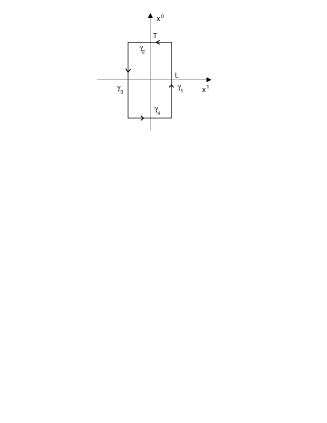
Figure 1.1: Parameterization of the closed rectangular loop $\gamma$ in four segments $\gamma_{i}$.

It is easy to show that the perturbative expansion of ${\cal W}_{\Gamma_{0}}$ is an even power series in the coupling constant, so that we can write

$${\cal W}_{\Gamma_{0}}=1+g^{2}{\cal W}^{(1)}+g^{4}{\cal W}^{(2)}+{\cal O}(g^{6})\ .$$ (1.39)

The advantage of using Wilson loop as a test of gauge invariance with respect to another gauge invariant quantity, the scattering amplitude (perturbative $S$-matrix elements), is at least twofold:

• in the non–Abelian case, the perturbative $S$-matrix is only formally defined due to the occurrence of severe infrared singularities on–shell;

• to a given order in the coupling constant, the computation of the graphs coming from the perturbative expansion of the Wilson loop is much easier than the ones of the corresponding $S$–matrix elements.

Another important symmetry of Yang–Mills theories in the two–dimensional case is their invariance under area preserving diffeomorphisms. The general reason for this fact, first emphasized by Witten [14], is that the field strength is a two-form in two dimensions. The action is therefore invariant under all diffeomorphisms that preserve the volume element of the surface. Then, the Wilson loop is not only gauge–invariant, but is also invariant under these diffeomorphisms and depends only, in strictly $1+1$ dimensions, from the area of the loop, no matter the orientation and the shape of the path.

It is possible to derive [37, 38] that the asymptotic behavior of the Wilson loop at fixed $L$ is

$$\lim_{T\to\infty}{\cal W}(L,T)=const.\ e^{-2iTV(2L)}\ ,$$ (1.40)

where $V(2L)$ is the potential between a “static” ${\rm q}{\rm\bar{q}}$ pair in the fundamental representation, separated by a distance $2L$, and the Wilson loop is the one in Fig. 1.1, one side along the space direction and one side along the time direction, of length $2L$ and $2T$ respectively.

As a matter of fact, in the strictly two–dimensional case, it is possible to express in closed form the expectation value of the Wilson loop, summing all the contributes in the perturbative series. When it is not possible, we will investigate its asymptotic behavior up to the $g^{4}$ order. The tests we are going to accomplish represent only necessary but, in general, not sufficient conditions to verify the correctness of the quantization scheme within the assigned subsidiary condition and, in particular, of the prescription we use for the spurious poles. In order to perform the test in the framework of the perturbation theory, we consider the expansion of the exponential:

$$\exp(-2iTV)=1-2iTV-2T^{2}V^{2}+\ldots.$$ (1.41)

The potential $V(2L)$ may be developed, in turn, as a perturbative series in $g^{2}$, namely

$$V=g^{2}V_{1}+g^{4}V_{2}+\ldots.$$ (1.42)

A necessary condition to get the exponential behavior of the Wilson loop reads that the coefficient of $T^{2}$ at the order $g^{4}$ is one–half the square of the linear coefficient in $T$ at the order $g^{2}$; this is equivalent to the cancellation of the non–Abelian terms increasing like $T^{2}$ (or worse) in the large $T$–limit. In order to explain this fact, we first recognize as non–Abelian terms in the perturbative expansion of the Wilson loop the ones proportional to the factor $f^{abc}f^{abc}=C_{A}(N^{2}-1)$, where $C_{A}$ is the Casimir factor in the adjoint representation of $SU(N)$. The above mentioned equivalence is clear, once we realize that all the terms linear in $T$ at the order $g^{2}$ are Abelian. Hence, for any diagram coming from the perturbative expansion of the Wilson loop, we shall only deal with its non–Abelian contributions behaving, at the order $g^{4}$, as $T^{2}$ (or worse) in the asymptotic limit. In order to obtain the expected exponential behavior, the sum of those contribution must vanish up to order $g^{4}$. As we already pointed out, the test of the exponential behavior, in the large $T$–limit, of the Wilson loop ${\cal W}_{\Gamma_{0}}$ is a necessary although not sufficient condition to check the gauge relativity principle, namely that in the perturbative quantum field theories different gauge choices must yield equivalent descriptions of the physical phenomena, i.e. the same value of gauge–invariant quantities.

The aim of this test is clear: as the exponential behavior of the Wilson loop (or, better, the cancellation up to $g^{4}$ of the non–Abelian terms behaving like $T^{2}$ or worse) is a necessary condition for the gauge invariance, if it is not reproduced within a given gauge choice, then the corresponding formulation of the perturbation theory turns out to be poorly defined. Therefore the results of this test, performed in particular in Chapter 3, will be crucial to check the soundness of the perturbative approach with different choices of gauge and to compare the different results obtained.

Chapter 2 Light-like Wilson Loop

We have seen in Chapter 1 that Yang–Mills theory without fermions in two dimensions is, in ’t Hooft approach, a free theory. This feature is at the root of the possibility of calculating the mesonic spectrum in the large N approximation [8, 39], when quarks are introduced.

Still difficulties in performing a Wick’s rotation in those conditions have been pointed out [11], and a causal prescription for the infrared singularity has been advocated, leading to a quite different solution for the vector propagator. In this context the bound state equation with vanishing bare quark masses [12] has solutions with quite different properties, when compared with the ones of refs. [8, 39].

In view of the above mentioned controversial results and of the fact that “pure” Yang–Mills theory does not immediately look free in Feynman gauge, where degrees of freedom of a “ghost”–type are present, it was worth performing a test [5] on a gauge invariant quantity: the review of this test is the subject of Chapter 2.

Following [5], we choose a rectangular Wilson loop with light–like sides, directed along the vectors $n_{\mu}=(T,-T)$ and $n^{*}_{\mu}=(L,L)$, with $L,T>0$, parameterized according to the equations:

$$C_{1} : x^{\mu}_{1}(t)=(tL,-tL)=n^{*\mu}t,$$

$$C_{2} : x^{\mu}_{2}(t)=(L+tT,-L+tT)=n^{*\mu}+n^{\mu}t,$$

$$C_{3} : x^{\mu}_{3}(t)=(T+L-tL,T-L+tL)=n^{\mu}+n^{*\mu}(1-t),$$

$$C_{4} : x^{\mu}_{4}(t)=(T-tT,T-tT)=n^{\mu}(1-t),\qquad 0\leq t\leq 1\ ,$$ (2.1)

and with area

$${\cal A}_{C}=2LT\ .$$ (2.2)

This contour has been considered in refs. [40, 26] for an analogous test of gauge invariance in $1+3$ dimensions. Its light–like character forces a Minkowski treatment.

We will review a perturbative calculation up to ${\cal O}(g^{4})$; in so doing topological effects will not be considered. The computation was performed in Feynman gauge (Section 2.1) and in light-cone gauge (Section 2.2), with Cauchy principal value prescription (Section 2.2.1) and Mandelstam–Leibbrandt prescription (Section 2.2.2) for the spurious pole in the vector propagator. We can anticipate the unexpected results that was obtained: the gauge invariant theory is not free at $d=1+1$, at variance with the commonly accepted behavior; the theory in $d=1+(D-1)$ is “discontinuous” in the limit $D\rightarrow 2$. Besides, two different, inequivalent formulations within the same choice of gauge, the light–cone gauge, seem to coexist: the Cauchy principal value and the Mandelstam–Leibbrandt formulations.

2.1 Light-like Wilson Loop in Feynman Gauge

In Feynman gauge already the free vector propagator does not exist as a tempered distribution in $1+1$ dimensions. A regularization is thereby mandatory and we choose to adopt the dimensional regularization, which preserves gauge invariance:

$$D^{F}_{\mu\nu}(x)=-g_{\mu\nu}{\pi^{-D/2}\over 4}\Gamma(D/2-1)(-x^{2}+i\epsilon)^{1-D/2},$$ (2.3)

The calculation in Feynman gauge of the light–like Wilson loop (2), in $1+(D-1)$ dimensions up to ${\cal O}(g^{4})$ has been performed in ref. [40]. Actually in ref. [40] part of the contribution from graphs containing three vector lines, has only been given as a Laurent expansion around $D=4$, owing to its complexity. In the following we shall exhibit its general expression in terms of a generalized hypergeometric series and then we shall expand it around $D=2$. We only report the final results concerning the contributions of the various diagrams.

The single vector exchange $({\cal O}(g^{2})$) gives

$${\cal W}_{F}^{(1)}=-\frac{1}{{\pi}^{2}}C_{F}{\Gamma(D/2-1)\over(D-4)^{2}}{\cal C},$$ (2.4)

where $C_{F}$ is the Casimir operator of the fundamental representation of color $SU(N)$ and

$${\cal C}\equiv\Bigl{[}(2\pi{\cal A}_{C}+i\epsilon)^{2-D/2}+(-2\pi{\cal A}_{C}+i\epsilon)^{2-D/2}\Bigr{]}.$$ (2.5)

One immediately notices that the propagator pole at $D=2$ is cancelled after integration over the contour, leading to a finite result.

There are a lot of Feynman diagrams contributing to the Wilson loop expectation value at order ${\cal O}(g^{4})$ of perturbation theory. However, the number of diagrams one has to evaluate could be drastically reduced using the non–Abelian exponentiation theorem [41, 42]. According to this theorem

$${\cal W}_{C}\equiv 1+\sum_{n=1}^{\infty}g^{2n}{\cal W}^{(n)}=\exp\sum_{n=1}^{\infty}w^{(n)},$$ (2.6)

where $w^{(n)}$ is given by the contribution of ${\cal W}^{(n)}$ with the maximal non–Abelian color factor to the order ${\cal O}(g^{2n})$ of perturbation theory, which is equal to $C_{F}$ for $n=1$ and $C_{F}C_{A}$ for $n=2$, where $C_{A}$ is the Casimir operator of the adjoint representation.

In so doing, at order ${\cal O}(g^{4})$ we could restrict ourselves to the “maximally non–Abelian” contributions proportional to $C_{F}C_{A}$. In fact, the terms proportional to $C_{F}C_{A}$ and to $C_{F}$ are distinct and cannot mix. The test reported in this chapter is concerned only with the non–Abelian terms. Instead, in the next chapter our attitude will be to compare the terms proportional to $C_{F}C_{A}$ and to verify explicitly that, at order ${\cal O}(g^{4})$, the terms proportional to $C_{F}$ are those that we expect from the ${\cal O}(g^{2})$ computation using the non–Abelian exponentiation theorem. The computation of the (Abelian) terms proportional to $C_{F}$ will be only a further check of the internal consistency of our results, but in all cases the significant test of gauge invariance will be given by the $C_{F}C_{A}$ term.

The diagrams contributing to order ${\cal O}(g^{4})$ can be grouped into three distinct families:

• the ones in which the gluon propagator contains a self–energy correction;

• the ones with a double gluon exchange in which the propagators can either cross or uncross;

• the ones involving a triple vector vertex.

In strictly two dimensions and in an axial gauge only the second family is present. But in Feynman gauge all of them must be taken into account; moreover we are here considering the problem in $D$–dimensions. The second family is also the only one contributing to the Abelian case.

We start by considering the diagrams belonging to the first category.

The self–energy correction to the propagator gives

$${\cal W}_{F}^{(2;se)}={C_{F}C_{A}\over{64{\pi}^{4}}}{\Gamma^{2}(D/2-1)(3D-2)\over(D-4)^{3}(D-3)(D-1)}{\cal E},$$ (2.7)

where

$${\cal E}\equiv\Bigl{[}(2\pi{\cal A}_{C}+i\epsilon)^{4-D}+(-2\pi{\cal A}_{C}+i\epsilon)^{4-D}\Bigr{]}$$ (2.8)

and the fermionic loop has not been considered (pure Yang–Mills theory). Eq. (2.7) exhibits a double pole at $D=2$.

Next we consider the contribution of the so–called “cross” graphs, the ones with two non interacting crossed vector exchanges

$${\cal W}_{F}^{(2;cr)}=-{C_{F}C_{A}\over{16{\pi}^{4}}}{\Gamma^{2}(D/2-1)\over(D-4)^{4}}\left[{\cal E}+8{\cal B}\left(1-{\Gamma^{2}(3-D/2)\over\Gamma(5-D)}\right)\right],$$ (2.9)

where

$${\cal B}\equiv\Bigl{[}(2\pi{\cal A}_{C}+i\epsilon)(-2\pi{\cal A}_{C}+i\epsilon)\Bigr{]}^{2-D/2}.$$ (2.10)

Again a double pole occurs at $D=2$.

The contribution coming from graphs with three vector lines is by far the most complex one. It is convenient to split it into two parts, one coming from graphs with two vector lines attached to the same side

$${\cal W}_{F}^{(2;ss)} = {C_{F}C_{A}\over{16{\pi}^{4}}}{{\cal E}\over(D-4)^{4}}\bigg{[}2\Gamma(3-D/2)\Gamma(D/2-1)\Gamma(D-3)$$ (2.11)

$$- {1\over D-3}\Gamma^{2}(D/2-1)\bigg{]}$$

and another one in which the three “gluons” end in three different rectangle sides

$${\cal W}_{F}^{(2;ds)}={C_{F}C_{A}\over{64{\pi}^{4}}}{\cal E}\left\{{\Gamma^{2}(D/2-2)\Gamma(4-D/2)\Gamma(D-3)\over\Gamma(D/2)}F(D)\right.$$

$$+\left.{4\over(D-4)^{4}}\Bigl{[}\Gamma(3-D/2)\Gamma(D/2-1)\Gamma(D-3)-\Gamma^{2}(D/2-1)\Bigr{]}\right\}.$$ (2.12)

The function $F(D)$ is defined as

$$F(D)=S(D)+{D/2-1\over(3-D/2)(D-4)}\Big{[}5\psi(3-D/2)-\psi(D/2-1)$$

$$-2\psi(1)-2\psi(5-D)\Big{]},$$ (2.13)

$\psi(D)$ being the digamma function and $S(D)$ the convergent generalized hypergeometric series

$$S(D)=\sum^{\infty}_{n=0}{1\over(n+1)^{2}}{1\over n!}{\Gamma(n+D-3)\over\Gamma(D-3)}{\Gamma(n+4-D/2)\over\Gamma(4-D/2)}{\Gamma(D/2)\over\Gamma(n+D/2)}.$$ (2.14)

Both contributions exhibit a double pole at $D=2$. The Laurent expansion of eq. (2.1) around $D=4$, reproduces exactly the expression given in ref. [40].

Summing eqs. (2.7), (2.9), (2.11) and (2.1) and performing a careful Laurent expansion around $D=2$, it is tedious but straightforward to prove that double and single poles cancel, leaving only the finite contribution

$${\cal W}_{F}^{(2)}(D=2)=\frac{C_{F}C_{A}{\cal A}_{C}^{2}}{16{\pi}^{2}}\left(1+{\pi^{2}\over 3}\right).$$ (2.15)

The presence of a non vanishing $C_{F}C_{A}$ contribution is a dramatic result: it means that the theory does not exponentiate in an Abelian way, as a “bona fide” free theory should do. In order to better understand this result, it is worth turning now our attention to the same Wilson loop calculation, performed in the light–cone axial gauge $n\cdot A=0$.

2.2 Light-like Wilson Loop in Light-Cone Gauge

We have seen in Section 1.2.1 and 1.2.2 that, once we have chosen the light-cone gauge, it is possible to adopt two different prescriptions for the pole of the vector propagator in $1+1$ dimensions:

• the so-called manifestly unitary formulation, or Cauchy principal value prescription;

• the causal formulation, or Mandelstam-Leibbrandt prescription.

In this section we will compare these two formulations to the result of the previous section, obtained in Feynman gauge. The light–like character of the Wilson loop leads to the vanishing of a lot of Feynman diagrams, thus simplifying the computation.

2.2.1 Cauchy Principal Value Prescription

In this section we stick in $1+1$ dimensions, since CPV prescription is well defined only in this case. If we interpret $x^{+}$ as time direction, the field $A_{+}$ is not an independent dynamical variable and just provides a non–local force of Coulomb type between fermions. In momentum space it can be described by the “exchange” $k_{-}^{-2}$ [8, 10], where $k_{-}^{-2}$ has to be interpreted as in eq. (1.8):

$$D_{++}^{CPV}(x)=-{i\over(2\pi)^{2}}\int e^{ikx}d^{2}k{\partial\over\partial k_{-}}\left[\textrm{P}\left({1\over k_{-}}\right)\right]=-{i\over 2}|x^{-}|\delta(x^{+}).$$ (2.16)

It is straightforward to check that, by inserting eq. (2.16) in our Wilson loop, the result (2.4) at ${\cal O}(g^{2})$ is recovered.

At ${\cal O}(g^{4})$ in $1+1$ dimensions, the only “a priori” surviving non–Abelian contribution, which is due to “cross” graphs, vanishes using eq. (2.16) (see Appendix D). Henceforth no $C_{F}C_{A}$ term appears, in agreement with Abelian exponentiation, but at variance with the result obtained (after regularization!) in Feynman gauge. The sum of the perturbative series easily gives:

$${\cal W}_{CPV}=\exp\left(-{i\over 2}C_{F}g^{2}{\cal A}_{C}\right)\ .$$ (2.17)

On the other hand no fully consistent vector loop calculation would be feasible in $1+(D-1)$ dimensions, using a CPV prescription or introducing infrared cutoffs [21].

2.2.2 Mandelstam-Leibbrandt Prescription

The free vector propagator in light–cone gauge is very sensitive to the prescription used to handle the so–called “spurious” singularity. The only prescription which allows to perform a Wick’s rotation without extra terms and to calculate loop diagrams in a consistent way [27] is the causal Mandelstam–Leibbrandt (ML) prescription [23, 24]. In a canonical formalism it is obtained by imposing equal time commutation relations [19]; in two dimensions a “ghost” degree of freedom still survives, as extensively discussed in Section 1.2.2. When ML prescription is adopted, the free vector propagator is indeed a tempered distribution at $D=2$ [43], at variance with its behavior in Feynman gauge. In particular, when $x_{\perp}=0$,

$$D_{++}^{ML}(x)={2\pi^{-D/2}\Gamma(D/2)\over 4-D}{(x^{-})^{2}\over(-x^{2}+i\epsilon)^{D/2}}.$$ (2.18)

The calculation of the Wilson loop under consideration at ${\cal O}(g^{4})$ in $1+(D-1)$ dimensions, using light–cone gauge with Mandelstam–Leibbrandt prescription, has been performed in ref. [26]. Here we shall report those results and then perform their Laurent expansion around $D=2$, the value we are interested in.

One might wonder why dimensional regularization should be introduced at all, as one might presume that single graph contributions are likely to be finite in this gauge. On the other hand, while remaining strictly at $D=2$, no self–interaction should be present. These arguments are true, but the dimensional approach is necessary to make a complete comparison between the Mandelstam–Leibbrandt results and the Feynman ones.

In fact, the calculation ${\cal O}(g^{2})$ is easily performed and the result exactly coincides with eq. (2.4), for any value of $D$. Therefore at ${\cal O}(g^{4})$ we again confine ourselves to the “maximally non–Abelian” contributions, without losing information. The self–energy graph now gives

$${\cal W}_{ML}^{(2;se)}={C_{F}C_{A}\over{16{\pi}^{4}}}{\cal E}\bigg{\{}{4\over(4-D)^{4}(D-3)}\bigg{[}{\Gamma^{2}(3-D/2)\Gamma(D-3)\over\Gamma(5-D)}$$

$$-\Gamma^{2}(D/2-1)\bigg{]}+{\Gamma^{2}(D/2-1)\over(4-D)^{3}(D-3)}\bigg{[}3-{3D-2\over 4(D-1)}-{D-2\over D-3}\bigg{]}\bigg{\}}.$$ (2.19)

Its limit at $D=2$

$${\cal W}_{ML}^{(2;se)}(D=2)=\frac{C_{F}C_{A}{\cal A}_{C}^{2}}{{16{\pi}^{2}}}$$ (2.20)

is finite, but it does not vanish, as one might have naively expected.

We shall discuss this point at the end of the section. For the time being let us recall that, when $D\not=2$, “transverse” vector components are turned on and, although their contribution is expected to be ${\cal O}(D-2)$, it can compete with singularities arising from loop corrections. This is indeed what happens in the self–energy calculation.

Similarly the contribution from the “cross” graphs

$${\cal W}_{ML}^{(2;cr)}=-{C_{F}C_{A}\over{16{\pi}^{4}}}{\Gamma^{2}(D/2-1)\over(D-4)^{4}}\left\{2{\cal E}{D-2\over D-3}+8{\cal B}\left[1-2{\Gamma^{2}(3-D/2)\over\Gamma(5-D)}\right]\right\}$$ (2.21)

leads to a finite, non vanishing, result in the limit $D=2$

$${\cal W}_{ML}^{(2;cr)}(D=2)=\frac{C_{F}C_{A}{\cal A}_{C}^{2}}{48}\ .$$ (2.22)

Summing eqs. (2.20) and (2.22) we exactly recover eq. (2.15).

As a matter of fact the contribution due to graphs with three “gluon” lines [26]

$${\cal W}_{ML}^{(2;3g)} = \Omega\left\{\Gamma(D/2-2)\Gamma(3-D/2)+{\Gamma^{2}(3-D/2)\over\Gamma(5-D)}{6D-28\over(D-2)(D-4)}\right.$$ (2.23)

$$- \left.{2\over\Gamma(2-D/2)}S_{1}(D)-(4-D)\Gamma(3-D/2)S_{2}(D)\right\}$$

where

$$\Omega={2C_{F}C_{A}\over(2\pi)^{D}}(2{\cal A}_{C})^{4-D}e^{-i\pi D\over 2}\cos\left({\pi D\over 2}\right){\Gamma(D-4)\over(D-4)^{2}},$$ (2.24)

$$S_{1}(D)=\sum^{\infty}_{n=0}{\Gamma(n+2-D/2)\over(n+3-D/2)n!}\left[{2\over(n+D/2-1)(n+D/2)}+{1\over n+3-D/2}\right.\\ \left.+\psi(n+D/2)-\psi(n+3-D/2)-{\Gamma(n+D/2-1)\Gamma(5-D)\over\Gamma(4+n-D/2)}\right]$$ (2.25)

and

$$S_{2}(D)=\sum^{\infty}_{n=0}{\Gamma(n+3-D/2)\over\Gamma(n+6-D)}\left[\Gamma(D/2-2)\left({\Gamma(n+5-D)\over\Gamma(n+3-D/2)}-{\Gamma(n+2)\over\Gamma(n+D/2)}\right)\right.\\ +\left.2{\Gamma(n+1)\Gamma(D/2)\over\Gamma(n+1+D/2)}+{\Gamma(n+5-D)\Gamma(D/2-1)\over\Gamma(n+4-D/2)}-{\Gamma(n+1)\Gamma(3-D/2)\over\Gamma(n+4-D/2)}\right]$$ (2.26)

vanishes when $D=2$.

As a consequence the same finite result for the Wilson loop ${\cal O}(g^{4})$ at $D=2$ is obtained both in Feynman and in light–cone gauges. However non–Abelian terms are definitely present; the theory cannot be considered a free one in quantum loop calculations at $D=2$, in spite of the quadratic nature of its classical Lagrangian density in light–cone gauge. From a practical view point, in this fully interacting theory, the hope of getting solutions, when quarks are included, e.g. for the mesonic spectrum, in analogy with ’t Hooft’s treatment, seems remote.

If we remain strictly in $1+1$ dimensions, neither self–energy corrections nor graphs with three vector lines should be considered, and we have only the contribution of crossed graphs (2.22). The result we obtain neither coincides with the one in Feynman gauge (the limit $D\rightarrow 2$ being “discontinuous”), as we have neglected the non–vanishing self–energy correction, nor obeys Abelian exponentiation as in CPV approach, the reason being rooted in a different content of the degrees of freedom (the ghost fields $\lambda^{a}$ of eq. (1.25)).

2.3 Concluding Remarks

The computation of the expectation value of the Wilson loop (2) gave the following unexpected results.

The ${\cal O}(g^{4})$ perturbative loop expression in $d=1+(D-1)$ dimensions is finite in the limit $D\to 2$. The results in Feynman and light–cone gauge (with Mandelstam–Leibbrandt prescription) coincide, as required by gauge invariance. They are function only of the area ${\cal A}_{C}$ for any dimension $D$ and exhibit also a dependence on $C_{A}$, the Casimir constant of the adjoint representation.

This dependence, when looked at in the light-cone gauge calculation, comes from non-planar diagrams with the colour factor $C_{F}(C_{F}-C_{A}/2)$. Besides, there is a genuine contribution proportional to $C_{F}C_{A}$ coming from the one-loop correction to the vector propagator. This is surprising at first sight, as in strictly $1+1$ dimensions the triple vector vertex vanishes in axial gauges. What happens is that transverse degrees of freedom, although coupled with a vanishing strength at $D=2$, produce finite contributions when matching with the self-energy loop singularity precisely at $D=2$, eventually producing a finite result. Such a dimensional “anomaly-type” phenomenon is responsible of the discontinuity of Yang–Mills theories at $D=2$, namely of the finite, non vanishing result of eq. (2.2.2) in the limit $D\to 2$.

Surely this phenomenon could not appear in a strictly $1+1$ dimensional calculation, which would only lead to the (smooth) non-planar diagram result. We stress that this contribution is essential to get agreement with the Feynman gauge calculation, in other words with gauge invariance.

We notice that no ambiguity affects our light-cone gauge results, which do not involve infinities; in addition the discrepancy cannot be accounted for by a simple redefinition of the coupling, that would also, while unjustified on general grounds, turn out to be dependent on the area of the loop.

In order to make the argument complete, we recall that a calculation of the same Wilson loop in strictly $1+1$ dimension in light-cone gauge with a CPV prescription for the “spurious” singularity produces a vanishing contribution from non–planar graphs. Only planar diagrams survive, leading to Abelian–like results depending only on $C_{F}$, which can be resummed to all orders in the perturbative expansion to recover the expected exponentiation of the area.

This result, which is the usual one found in the literature, although quite transparent, does neither coincide with the limit $D\to 2$ of the light–cone gauge result with ML prescription (which is in agreement with the limit $D\to 2$ in Feynman gauge), nor with the ML result in strictly two dimensions. The test cannot be generalized to $D\neq 2$ dimensions as CPV prescription is at odds with causality in this case [27].

What we can certainly state is the perturbative inequivalence of CPV and Mandelstam–Leibbrandt formulations. At this point, we have two inequivalent formulations of the same theory, the two–dimensional Yang–Mills theory, within the same gauge choice. Now, a natural question arises: is there any formulation that is clearly wrong, or are they both legitimate?

To answer to this question, we will study the transition from $D>2$ to $D=2$, both in Feynman gauge and in light–cone gauge with ML prescription, in order to test the soundness of our perturbative approach when we are going towards the two–dimensional case from higher dimensions. To do that, we will apply the criterion exposed at the end of Section 1.3, namely the Wilson loop exponentiation, therefore considering a different Wilson loop, viz a space–time rectangular loop rather than a light–like one. We already know that this Wilson loop, from a physical point of view, is even more interesting and provides also information about the interaction potential between a quark and an antiquark. These computations, that are the subject of the next chapter, will help us to understand the features of Yang–Mills theories in ML formulation.

Chapter 3 Space-Time Wilson Loop

In order to clarify whether the appearance at ${\cal O}(g^{4})$ of the maximally non–Abelian term (proportional to $C_{A}$) is indeed a pathology, one should examine the potential $V(2L)$ between a “static” ${\rm q}{\rm\bar{q}}$ pair in the fundamental representation, separated by a distance $2L$. Therefore in this chapter, following the refs. [6, 3, 4], we will consider a different Wilson loop, namely a rectangular loop with one side along the space direction and one side along the time direction, of length $2L$ and $2T$ respectively. Eventually the limit $T\to\infty$ at fixed $L$ is to be taken: the potential $V(2L)$ between the quark and the antiquark is indeed related to the value of the corresponding Wilson loop amplitude ${\cal W}(L,T)$ through the equation [37, 38]

$$\lim_{T\to\infty}{\cal W}(L,T)=const.\ e^{-2iTV(2L)}\ .$$ (3.1)

The crucial point to notice in eq.(3.1), as already discussed in Section 1.3, is that the dependence on the Casimir constant $C_{A}$ should cancel at the leading order when $T\to\infty$ in any coefficient of a perturbative expansion of the potential with respect to coupling constant. This criterion has often been used as a check of gauge invariance [27] and its failure has been considered as the proof of a sick formulation of four–dimensional theories [37]. Actually, at the end of our enquiry we will discover that the criterion is not satisfied just in the two–dimensional case. But here we will choose to have a more constructive attitude: in fact in the two–dimensional case it is possible to obtain exact non–perturbative results. Since they are at our disposal, we can proceed to a comparison with the results derived from our perturbative test. We could say that, in so doing, we check the behavior of our criterion, varying the dimension in which we are working, in the transition to $D\to 2$. There are some indications [44, 45] that support the conjecture that the failure of our perturbative criterion in the strictly two–dimensional case depends on the need of taking into account the non–perturbative contributions, rather than on inconsistencies in the perturbative ML formulation. Anyway, we will defer the discussion of this point until the Conclusions.

Then we choose the closed path $\gamma$ parameterized by the following four segments $\gamma_{i}$,

$$\gamma_{1} : x_{1}^{\mu}(s)=(sT,L)\ ,$$

$$\gamma_{2} : x_{2}^{\mu}(s)=(T,-sL)\ ,$$

$$\gamma_{3} : x_{3}^{\mu}(s)=(-sT,-L)\ ,$$

$$\gamma_{4} : x_{4}^{\mu}(s)=(-T,sL)\ ,\ \ \qquad-1\leq s\leq 1.$$ (3.2)

describing a (counterclockwise-oriented) rectangle centered at the origin of the plane ($x^{1},x^{0}$), with length sides $(2L,2T)$, respectively (see Fig. 1.1 at page 1.1) and with area

$${\cal A}_{\gamma}=4LT$$ (3.3)

To have a sensitive check of gauge invariance, one has to consider at least the order $g^{4}$, i.e. one has to evaluate ${\cal W}^{(2)}$, as this is the lowest order where genuinely non–Abelian $C_{F}C_{A}$ contributions may appear. In turn, in the calculation of ${\cal W}^{(2)}$, only the so called maximally non–Abelian contribution needs to be evaluated, that in our case comes from the terms proportional to $C_{F}C_{A}$. The Abelian contribution, proportional to $C_{F}^{2}$, can be easily obtained thanks to the non–Abelian exponentiation theorem [42] and will be computed explicitly as a further check of consistency.

In Section 3.1 we will proceed to the computation of the loop (3.2) in Feynman gauge, while in Section 3.2 we will choose light-cone gauge, respectively with CPV (Section 3.2.1) and with Mandelstam-Leibbrandt (Sections 3.2.2 and 3.2.3) prescriptions for the propagator pole. We can anticipate the main result of this chapter, namely that, in the large $T$-limit when $D>2$, the perturbative ${\cal O}(g^{4})$ contribution is proportional only to $C_{F}$, and does not contain terms proportional to $C_{A}$. If instead we compute the Wilson loop at $D=2$, the result depends also on $C_{A}$, a pure area law behavior is recovered, but the term proportional to $C_{A}$ survives also in the limit $T\to\infty$.

3.1 Space-Time Wilson Loop in Feynman Gauge

In this section we will compute the Wilson loop (3.2) in Feynman gauge [3], in the framework of dimensional regularization ($D=2\omega$).

An explicit evaluation of the function ${\cal W}^{(1)}$ in eq.(1.39) gives the diagrams contributing to the loop with a single exchange (i.e. one propagator), namely

$${\cal W}^{(1)}_{F}=-{1\over 2}C_{F}\oint\oint D_{\mu\nu}^{F}(x-y)dx^{\mu}dy^{\nu}\ ,$$ (3.4)

where $D_{\mu\nu}^{F}(x)$ is the usual free propagator (2.3) in Feynman gauge.

A fairly easy calculation leads to the result

$${\cal W}^{(1)}_{F}={{C_{F}}\over{{\pi}^{\omega}}}(2L)^{2-2\omega}LT\bigg{[}i\Gamma(\omega-3/2)\Gamma(1/2)\\ +{{2\beta\Gamma(\omega)}\over{\omega-2}}\left({1\over{3-2\omega}}-e^{-i\pi\omega}\sum_{n=1}^{\infty}{{\Gamma(n+\omega-2)}\over{\Gamma(\omega-2)}}{{\beta^{2n+2\omega-4}}\over{(2n-1)(2n+2\omega-3)n!}}\right)\bigg{]},$$ (3.5)

where $\beta=L/T$.

It should be noticed that this result does not coincide with the corresponding one of eq. (2.4), which was evaluated with the same gauge choice but with the loop sides along the $x^{+}$ and $x^{-}$ directions. Contrary to what happens in eq. (2.4), eq. (3.5) exhibits an explicit dependence on the ratio $\beta=L/T$. Only in the two dimensional limit the two results coincide: the limit $\omega\to 1$ is smooth and restores the pure area dependence

$${\cal W}^{(1)}_{F}(D=2)=-\frac{i}{2}C_{F}{\cal A}_{\gamma}.$$ (3.6)

As in Section 2.1, the diagrams contributing to ${\cal W}^{(2)}_{F}$ can be grouped into three distinct families

$${\cal W}^{(2)}_{F}={\cal W}^{(2;2g)}_{F}+{\cal W}^{(2;se)}_{F}+{\cal W}^{(2;3g)}_{F}\ :$$ (3.7)

• the ones with a double gluon exchange in which the propagators can either cross or uncross;

• the ones in which the gluon propagator contains a self–energy correction;

• the ones involving a triple vector vertex.

In strictly two dimensions and in an axial gauge only the first family is present, but in Feynman gauge all of them must be taken into account; moreover we are here considering the problem in $D$-dimensions, because of the dimensional regularization. The first family is also the only one contributing to the Abelian case.

a. Exchange Diagrams in Feynman Gauge

We start by considering the diagrams belonging to the first category, namely the ones with a double gluon exchange. A straightforward calculation gives

$${\cal W}^{(2;2g)}_{F}={1\over 8N}\oint\!\!\!\oint\!\!\!\oint\!\!\!\oint{\rm Tr}[{\cal P}(T^{a}_{x}T^{a}_{y}T^{b}_{z}T^{b}_{w})]D_{\mu\nu}(x-y)D_{\rho\sigma}(z-w)\;dx^{\mu}dy^{\nu}dz^{\rho}dw^{\sigma}\;\;,\\ {}$$ (3.8)

where subscripts in the matrices have been introduced to specify their ordering. From eq. (LABEL:w4), the diagrams with two-gluons exchanges contributing to the order $g^{4}$ in the perturbative expansion of the Wilson loop fall into two distinct classes, depending on the topology of the diagrams:

1. Non-crossed diagrams: if the pairs $(x,y)$ and $(z,w)$ are contiguous around the loop the two propagators do not cross (see Fig. 3.1a) and the trace in (LABEL:w4) gives

   $${\rm Tr}[T^{a}T^{a}T^{b}T^{b}]=NC_{F}^{2};$$ (3.9)

2. Crossed diagrams: if the pairs $(x,y)$ and $(z,w)$ are not contiguous around the loop the two propagators do cross (see Fig. 3.1b) and the trace in (LABEL:w4) gives

   $${\rm Tr}[T^{a}T^{b}T^{a}T^{b}]={\rm Tr}[T^{a}(T^{a}T^{b}+[T^{b},T^{a}])T^{b}]=N(C_{F}^{2}-(1/2)C_{A}C_{F}),$$ (3.10)

   $C_{A}$ being the Casimir constant of the adjoint representation defined by $f^{abc}f^{dbc}=C_{A}\delta^{ad}$.

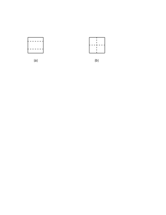
Figure 3.1: Example of non-crossed and crossed diagrams.

We see that the $C_{F}^{2}$ term is present in both types of diagrams and with the same coefficient. This term is usually denoted “Abelian term”: were the theory Abelian, only such $C_{F}^{2}$ terms would contribute to the loop. On the other hand, the $C_{F}C_{A}$ term is present only in crossed diagrams and is typical of non–Abelian theories.

Thus, we can decompose ${\cal W}^{(2;2g)}_{F}$ as the sum of an Abelian and a non–Abelian part,

$${\cal W}^{(2;2g)}_{F}={\cal W}^{(2;ab)}_{F}+{\cal W}^{(2;na)}_{F}\ .$$ (3.11)

Moreover, the Abelian part is simply half of the square of the order-$g^{2}$ term, i.e.

$${\cal W}^{(2;ab)}_{F} = {1\over 8}C_{F}^{2}\oint\oint\oint\oint D_{\mu\nu}^{F}(x-y)D_{\rho\sigma}^{F}(z-w)\;dx^{\mu}dy^{\nu}dz^{\rho}dw^{\sigma}$$ (3.12)

$$= {1\over 2}\left(-{1\over 2}C_{F}\oint\oint D_{\mu\nu}^{F}(x-y)dx^{\mu}dy^{\nu}\right)^{2}\ \ .$$

This result at ${\cal O}(g^{4})$ has been explicitly checked calculating the relevant non-crossed exchange diagrams (see Appendix A for details).

Equation (3.12) agrees with the non–Abelian exponentiation theorem, which tells us that the Abelian terms (depending only on $C_{F}$) in the perturbative expansion of the Wilson loop sum up to reproduce the Abelian exponential

$${\cal W}_{F}^{ab}(L,T)={\rm exp}\left(-{1\over 2}C_{F}g^{2}\oint\oint D^{F}_{\mu\nu}(x-y)dx^{\mu}dy^{\nu}\right)\ ,$$ (3.13)

where the result in eq.(3.5) can be introduced.

In the limit $D\to 2$ the simple exponentiation of the area is easily recovered

$${\cal W}_{F}^{ab}(L,T)=\exp\left(-{i\over 2}C_{F}g^{2}{\cal A}_{\gamma}\right)\ .$$ (3.14)

We have now to calculate loop integrals of the type given in eq.(LABEL:w4). In view of the parameterization (3.2), it is convenient to decompose loop integrals as sums of integrals over the segments $\gamma_{i}$, and to this purpose we define

$$E_{ij}^{F}(s,t)=D_{\mu\nu}^{F}\bigl{[}\gamma_{i}(s)-\gamma_{j}(t)\bigr{]}\dot{\gamma}_{i}^{\mu}(s)\dot{\gamma}_{j}^{\nu}(t)\ ,\qquad i,j=1,\dots,4\ \,,$$ (3.15)

where the dot denotes the derivative with respect to the variable parameterizing the segment. In this way, each diagram can be written as integrals of products of functions of the type (3.15). Each graph will be labelled by a set of pairs $(i,j)$, each pair denoting a gluon propagator joining the segments $\gamma_{i}$ and $\gamma_{j}$.

Due to the symmetric choice of the contour $\gamma$ and to the fact that propagators are even functions, i.e. $D_{\mu\nu}^{F}(x)=D_{\mu\nu}^{F}(-x)$, we have the following identities that halve the number of diagrams to be evaluated:

$$E_{ij}^{F}(s,t) = E_{ji}^{F}(t,s)\ ,$$

$$E_{11}^{F}(s,t) = E_{33}^{F}(s,t)\ ,$$

$$E_{22}^{F}(s,t) = E_{44}^{F}(s,t)\ .$$ (3.16)

We remind the reader that in Feynman gauge the propagators can attach either to the same rectangle side or to opposite sides, but not on a couple of contiguous ones.

We have now to consider the ${\cal O}(g^{4})\ C_{F}C_{A}$-terms coming from “crossed diagrams” (maximally non–Abelian ones), that need to be evaluated

$${\cal W}^{(2;na)}_{F} = -{1\over 2}C_{A}C_{F}\sum_{i,j,k,l}{}^{{}^{\prime}}\int ds\int dt\int du\int dv\ E_{ij}^{F}(s,t)E_{kl}^{F}(u,v)$$ (3.17)

$$\equiv -{1\over 2}C_{A}C_{F}\sum_{i,j,k,l}{}^{{}^{\prime}}C_{(ij)(kl)}^{F}\ ,$$

where the primes mean that we have to sum only over crossed propagators configurations and over topologically inequivalent contributions, as carefully explained in the following; we have not specified the integration extrema as they depend on the particular type of crossed diagram we are considering (the extrema must be chosen in such a way that propagators remain crossed).

The last equality in eq. (3.17) defines the general diagram $C_{(ij)(kl)}^{F}$: it is a diagram with two crossed propagators joining the sides $(ij)$ and $(kl)$ of the contour (3.2). In Fig. 3.2 a few examples of diagrams are drawn to get the reader acquainted with the notation.

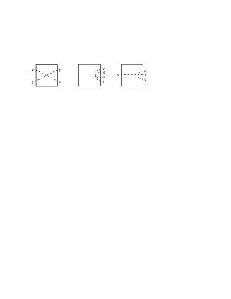
Figure 3.2: Examples of crossed diagrams; they are labelled as $C_{(13)(13)}$, $C_{(11)(11)}$ and $C_{(13)(11)}$, respectively

The first of eq. (3.16) permits to select just 11 types of topologically distinct crossed diagrams. The remaining symmetry relations (3.16) further lower the number to 7. As a matter of fact, although topologically inequivalent, from eq. (3.16) it is easy to get

$$C_{(11)(11)}^{F} =C_{(33)(33)}^{F}\ \ ,\qquad C_{(22)(22)}^{F}= C_{(44)(44)}^{F}\ \ ,$$

$$C_{(11)(13)}^{F} =C_{(33)(13)}^{F}\ \ ,\qquad C_{(22)(24)}^{F}= C_{(44)(24)}^{F}.$$ (3.18)

which are the 4 relations needed to lower the number of diagrams to be evaluated from 11 to 7. Besides the 8 diagrams quoted in eq. (3.18), there are three other crossed diagrams that do not possess any apparent symmetry relation with other diagrams: $C_{(13)(13)}^{F},\ C_{(24)(24)}^{F}$ and $C_{(13)(24)}^{F}$ (see Fig. 3.3), so that the number of topologically inequivalent crossed diagrams is indeed 11.

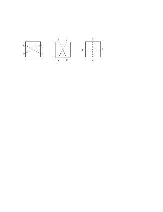
Figure 3.3: The three crossed diagrams that are unrelated to other diagrams through symmetry relations; they are $C_{(13)(13)}$, $C_{(24)(24)}$ and $C_{(13)(24)}$.

The calculation of the 7 independent diagrams needed is lengthy and not trivial. The details of such calculation are sketched in Appendix A. Each diagram depends not only on the area ${\cal A}_{\gamma}=4LT$ of the loop, but also on the dimensionless ratio $\beta=L/T$ through complicated multiple integrals.

Adding all the contributions as in eq. (3.17) we eventually arrive at the following result ${\cal O}(g^{4})$ for the non–Abelian part of the exchange diagrams contribution:

$${\cal W}^{(2;na)}_{F} = C_{F}C_{A}{{(2T)^{4-4\omega}}\over{\pi^{2\omega}}}(LT)^{2}e^{-2i\pi\omega}$$

$$\times\Big{(}{{\Gamma^{2}(\omega-1)}\over{(2\omega-4)(2\omega-3)}}\Big{[}1+{{1-\omega}\over{(4\omega-5)(2\omega-3)}}+{\cal O}(\beta^{5-4\omega})\Big{]}\Big{)}.$$

We notice that the expression above exhibits a double and a single pole at $\omega=1$, whose Laurent expansion gives

$${{\cal W}^{(2;na)}_{F}\pi^{2\omega}e^{2i\pi\omega}\over C_{F}C_{A}(2T)^{4-4\omega}(LT)^{2}}={1\over 2(\omega-1)^{2}}+{1-\gamma\over(\omega-1)}-1-2\gamma+\gamma^{2}+{\pi^{2}\over 12}+{\cal O}(\omega-1)\ ,\\ {}$$ (3.20)

$\gamma$ being the Euler-Mascheroni constant.

b. Bubble Diagrams in Feynman Gauge

We turn now our attention to the calculation of ${\cal W}^{(2;se)}_{F}$, namely of the diagrams with a single gluon exchange in which the propagator contains a self–energy correction ${\cal O}(g^{2})$. Of course both gluon and ghost contribute to the self–energy. The color factor is obviously a pure $C_{F}C_{A}$.

We call them “bubble” diagrams. We denote by $B_{ij}^{F}$ the contribution of the diagram in which the propagator connects the rectangle segments $\gamma_{i}$, $\gamma_{j}$ (see Fig. 3.4).

Figure 3.4: Examples of bubble diagrams. They are labelled as $B_{11}$, $B_{13}$ and $B_{34}$, respectively.

There are 10 topologically inequivalent diagrams; however, the symmetries we have already discussed and the symmetric choice of the contour entails the four conditions $B_{11}^{F}=B_{33}^{F}$, $B_{22}^{F}=B_{44}^{F}$, $B_{12}^{F}=B_{34}^{F}$, $B_{14}^{F}=B_{23}^{F}$, whereas the remaining two diagrams $B_{13}^{F}$ and $B_{24}^{F}$ are unrelated by any symmetry relation. In addition, it is easy to see by performing a simple change of variable that $B_{14}^{F}$ and $B_{34}^{F}$ are equal. Thus, there are 5 independent diagrams to be evaluated

$${\cal W}^{(2;se)}_{F}=B_{13}^{F}+B_{24}^{F}+2B_{11}^{F}+2B_{22}^{F}+4B_{12}^{F}.$$ (3.21)

The calculation is sketched in Appendix B. We here report the final result in the form of an expansion with respect to the variable $\beta$

$${\cal W}^{(2;se)}_{F} = C_{F}C_{A}{{(2T)^{4-4\omega}}\over{\pi^{2\omega}}}(LT)^{2}e^{-2i\pi\omega}\times$$

$$\Big{[}{{(3\omega-1)\Gamma^{2}(\omega)}\over{2\Gamma(2\omega)\Gamma(4-\omega)}}\Gamma(1-\omega)\Gamma(2\omega-2)\Big{(}{{2\omega-6}\over{5-4\omega}}+{\cal O}(\beta^{5-4\omega})\Big{)}\Big{]}.$$

Again we notice the presence of a double and of a single pole at $\omega=1.$ The relevant Laurent expansion is

$${{\cal W}^{(2;se)}_{F}\pi^{2\omega}e^{2i\pi\omega}\over C_{F}C_{A}(2T)^{4-4\omega}(LT)^{2}}=\\ ={1\over(\omega-1)^{2}}+{9-4\gamma\over 2(\omega-1)}+{39\over 2}-9\gamma+2\gamma^{2}+{\pi^{2}\over 6}+{\cal O}(\omega-1)\ ,\\$$ (3.23)

c. Spider Diagrams in Feynman Gauge

The third quantity ${\cal W}^{(2;3g)}_{F}$ is by far the most difficult one to be evaluated. It comes from “spider” diagrams, namely the diagrams containing the triple gluon vertex. We denote by $S_{ijk}^{F}$ the contribution of the diagram in which the propagators are attached to the segments $\gamma_{i}$, $\gamma_{j}$, $\gamma_{k}$ (see Fig. 3.5).

Figure 3.5: Examples of spider diagrams. They are labelled as $S_{123}$, $S_{112}$, respectively.

It can be checked that all the spiders with the three legs attached to the same line vanish, as well as the spiders with two legs on one side and the third leg attached to the opposite side, i.e. $S_{111}^{F}=S_{222}^{F}=S_{333}^{F}=S_{444}^{F}=S_{113}^{F}=S_{133}^{F}=S_{224}^{F}=S_{244}^{F}=0$. Thus, there are 12 non-vanishing topologically inequivalent diagrams; however, their number is just halved by the symmetric choice of the contour ($S_{124}^{F}=S_{234}^{F}$, $S_{123}^{F}=S_{134}^{F}$, $S_{112}^{F}=S_{334}^{F}$, $S_{233}^{F}=S_{114}^{F}$, $S_{344}^{F}=S_{122}^{F}$, $S_{144}^{F}=S_{223}^{F}$), so that ${\cal W}^{(2;3g)}_{F}$ can be expressed in terms of the remaining 6 independent ones

$${\cal W}^{(2;3g)}_{F}=2S_{112}^{F}+2S_{123}^{F}+2S_{124}^{F}+2S_{233}^{F}+2S_{144}^{F}+2S_{344}^{F}.$$ (3.24)

Each term is represented by a multiple integral which cannot be evaluated for a generic dimension $\omega$ in closed form. In particular it exhibits complicated analyticity properties in the variable $\beta$, just in the neighborhood of the value $\beta=0$ which is of interest for us. The main aspects of the calculation are again deferred to an Appendix (Appendix C).

We have succeeded in obtaining the following result for $D>2$

$$\lim_{\beta\to 0}{{\cal W}^{(2;3g)}_{F}\pi^{2\omega}e^{2i\pi\omega}\over C_{F}C_{A}(2T)^{4-4\omega}(LT)^{2}}=\\ =-{3\over 2(\omega-1)^{2}}+{3\gamma-11/2\over(\omega-1)}-{35\over 2}+11\gamma-3\gamma^{2}+{\pi^{2}\over 12}+{\cal O}(\omega-1)\ .\\$$ (3.25)

A double and a single pole at $D=2$ again are present in this expression.

* * *

Since the Abelian part of our results depends only on the Casimir constant $C_{F}$ and smoothly exponentiates in the large–$T$ limit even when $D>2$ (see eqs.(3.5,3.13)), in the following we focus our attention on the non-Abelian part, namely on the quantity containing the factor $C_{F}C_{A}$

$${\cal W}^{(2;na)}_{F}+{\cal W}^{(2;se)}_{F}+{\cal W}^{(2;3g)}_{F}.$$

It is actually convenient to divide by the square of the loop area, by introducing the new expression ${\cal N}$

$${\cal N}C_{F}C_{A}{\cal{A}_{\gamma}}^{2}={\cal W}^{(2;na)}_{F}+{\cal W}^{(2;se)}_{F}+{\cal W}^{(2;3g)}_{F}.$$ (3.26)

Then, from eqs. (3.1,3.1,LABEL:ragnilaurent), it is easy to conclude that, thanks to the factor $T^{4-4\omega}$, ${\cal N}$ vanishes in the limit $T\to\infty$ when $\omega>1$.

This is precisely the usual necessary condition required at ${\cal O}(g^{4})$ in order to get agreement with Abelian–like time exponentiation when summing higher orders [27].

We cannot discuss the limit $\omega\to 1$ for generic (small) values of $\beta$ in our results as we are only able to master the expressions at $\beta=0$.

Nevertheless if we consider the quantity

$$\lim_{\omega\to 1}\lim_{\beta\to 0}(T^{4\omega-4}{\cal N})\ ,$$ (3.27)

we get a quite interesting result. Indeed double and simple poles at $\omega=1$ cancel in the sum, leading to

$$\lim_{\omega\to 1}\lim_{\beta\to 0}(T^{4\omega-4}{\cal N})={1\over{16\pi^{2}}}\left(1+{{\pi^{2}}\over 3}\right)\ ,$$ (3.28)

which exactly coincides with eq. (2.15).

This is, first of all, a formidable check of all our calculations, if we conjecture that the same result is obtained by performing the limit

$$\lim_{\beta\to 0}\lim_{\omega\to 1}{\cal N}\ .$$ (3.29)

But it also entails the quite non trivial consequences we are going to discuss in Section 3.3. But first we will review the corresponding calculations in light–cone gauge.

3.2 Space-Time Wilson Loop in Light-Cone Gauge

In this section we will proceed to the computation of Wilson loop (3.2) in light-cone gauge, in order to compare the results obtained with the ones in Feynman gauge. We will review the computations done in $D=2$ with Cauchy principal value prescription (Section 3.2.1), and with Mandelstam–Leibbrandt prescription (Section 3.2.2), following ref. [6]. At the end we will complete the two–dimensional case, computing the self–energy contribution that arises in $D>2$ and that survives in the $D\to 2$ limit (Section 3.2.3).

3.2.1 Cauchy Principal Value Prescription

In this section we report the results of the computation of Wilson loop (3.2) in light-cone gauge with Cauchy principal value prescription. We shall begin with the ${\cal O}(g^{2})$ contribution. From eq. (3.4), using eqs. (3.2), (2.16), (3.15) and (3.16)(or, better, the analogous of eq. (3.16) for light–cone gauge, see eq. (3.34)) one can easily get

$${\cal W}_{CPV}^{(1)}=-{1\over 2}C_{F}\sum_{i,j=1}^{4}\int_{-1}^{1}ds\int_{-1}^{1}dt\ E_{ij}^{CPV}(s,t)=-{i\over 2}C_{F}{\cal A}_{\gamma}\ .$$ (3.30)

Once the ${\cal O}(g^{2})$ term is known, simple arguments permit to evaluate any order in the perturbative expansion, so that in this case the loop can be exactly obtained. Let us indeed consider the ${\cal O}(g^{4})$ term. As explained in the previous section, only the “genuine” non-Abelian part needs to be evaluated, i.e. the crossed diagrams containing the factor $C_{F}C_{A}$, as the Abelian part is already given by eq. (3.12), which in this case leads to

$${\cal W}_{CPV}^{(2;ab)}=-{1\over 8}C_{F}^{2}{\cal A}_{\gamma}^{2}\ .$$ (3.31)

However, due to the contact nature of the propagator in the CPV case, all the crossed diagrams trivially vanish so that ${\cal W}_{CPV}^{(2;na)}=0$: the $\delta(x^{+})$ term in the propagator only tolerates diagrams with parallel propagators, which therefore cannot cross, both in the Abelian and in the non-Abelian case. Obviously, this argument holds at any order in the perturbative expansion, so that only Abelian terms contribute and the sum of all of them, due to the Abelian exponentiation theorem, reproduces the exponential

$${\cal W}_{CPV}(L,T)={\rm exp}\left(-{i\over 2}g^{2}C_{F}{\cal A}_{\gamma}\right)\ .$$ (3.32)

A detailed discussion of this point can be found in Appendix D.

Consequently, from eq. (3.1), null plane light-cone quantization provides a linear confining potential for a quark–antiquark pair, with string tension $\sigma=g^{2}C_{F}/2$. This is the very same result one would have obtained in an Abelian theory, apart from the factor $C_{F}$. In this sense null plane light-cone gauge quantization provides a “free” theory: the Wilson loop does not feel the non-Abelian colour structure of the theory. This result, obtained in a Minkowskian framework, is in agreement with analogous Euclidean calculations [46].

3.2.2 Mandelstam-Leibbrandt Prescription ($D=2$)

In strictly $D=2$ the contribution to the expectation value of Wilson loop (3.2) is only given by Feynman diagrams with double gluon exchange, in which the propagators are crossed or uncrossed, as already discussed for the light–like contour. The analysis of the diagrams is similar to the one developed in Feynman gauge. The only difference is that we shall use the Mandelstam-Leibbrandt propagator for $D=2$:

$$D_{++}^{(ML)cd}(x)=D_{++}^{ML}(x)\delta^{cd}={i\delta^{cd}\over\pi^{2}}\int d^{2}k\,e^{ikx}{k_{+}^{2}\over(k^{2}+i\epsilon)^{2}}={\delta^{cd}\over\pi}{(x^{-})^{2}\over(-x^{2}+i\epsilon)}\$$ (3.33)

instead of Feynman propagator (2.3) in $D$ dimensions.

The fact that we are in strictly $1+1$ dimensions greatly simplifies the perturbative expansion (1.38), as the complete Green functions appearing in it become products of free propagators.

We will again use the definition (3.15), with the same notations of the Feynman case. Due to the symmetric choice of the contour $\gamma$ and to the fact that propagators are even functions, i.e. $D_{\mu\nu}^{ML}(x)=D_{\mu\nu}^{ML}(-x)$, we have the following identities that halve the number of diagrams to be evaluated:

$$E_{ij}^{ML}(s,t) = E_{ji}^{ML}(t,s)\ ,$$

$$E_{12}^{ML}(s,t) = E_{34}^{ML}(s,t)\ ,$$

$$E_{23}^{ML}(s,t) = E_{41}^{ML}(s,t)\ ,$$

$$E_{11}^{ML}(s,t) = E_{33}^{ML}(s,t)\ ,$$

$$E_{22}^{ML}(s,t) = E_{44}^{ML}(s,t)\ .$$ (3.34)

At variance with the Feynman case (3.16), here also diagrams with propagators attaching on a couple of contiguous sides contribute to the final result, thus leading to a more cumbersome computation. We begin with the ${\cal O}(g^{2})$ terms. Following the notation introduced in the previous section, ${\cal W}_{ML}^{(1)}$ can be written as the sum of 16 diagrams

$${\cal W}_{ML}^{(1)} = -{1\over 2}C_{F}\sum_{i,j=1}^{4}\int_{-1}^{1}ds\int_{-1}^{1}dtE_{ij}^{ML}(s,t)$$ (3.35)

$$\equiv -{1\over 2}C_{F}\sum_{i,j=1}^{4}C_{ij}^{ML}\ .$$

Thanks to the symmetry properties (3.34), only 6 of them are independent, and an explicit evaluation gives

$$\begin{split}C_{11}^{ML}&=C_{33}^{ML}=\frac{L^{2}}{\pi}\;\left(-\frac{1}{\beta^{2}}\right)\;\;\\ C_{22}^{ML}&=C_{44}^{ML}=\frac{L^{2}}{\pi}\;\;\\ C_{12}^{ML}&=C_{21}^{ML}=C_{34}^{ML}=C_{43}^{ML}=\frac{L^{2}}{\pi}\left[i\pi-\ln(\beta)+\left(1-\frac{1}{\beta^{2}}\right)\ln(1-\beta)\right]\;\;\\ C_{14}^{ML}&=C_{41}^{ML}=C_{23}^{ML}=C_{32}^{ML}=\frac{L^{2}}{\pi}\left[-\ln(\beta)+\left(1-\frac{1}{\beta^{2}}\right)\ln(1+\beta)\right]\;\;\\ C_{13}^{ML}&=C_{31}^{ML}=\frac{L^{2}}{\pi}\bigg{[}\frac{1}{\beta^{2}}+\left(\frac{2}{\beta}-2\right)i\pi+4\ln(\beta)-\left(\frac{2}{\beta}+2\right)\ln(1+\beta)\\ &+\left(\frac{2}{\beta}-2\right)\ln(1-\beta)\bigg{]}\;\;\\ C_{24}^{ML}&=C_{42}^{ML}=\frac{L^{2}}{\pi}\left[-1+\left(\frac{2}{\beta^{2}}+\frac{2}{\beta}\right)\ln(1+\beta)+\left(\frac{2}{\beta^{2}}-\frac{2}{\beta}\right)\ln(1-\beta)\right]\;\;\ \\ \end{split}$$ (3.36)

Summing up all the coefficients (3.36) as in (3.35) one gets that the second–order calculation is

$${\cal W}_{ML}^{(1)}=-{i\over 2}C_{F}{\cal A}_{\gamma}\ .$$ (3.37)

The second–order calculation is in agreement with the CPV case (see eq. (3.30)). However, as often happens in Wilson loop calculations, an ${\cal O}(g^{2})$ computation is too weak a probe to check consistency and gauge invariance. Thus, we have to consider the ${\cal O}(g^{4})$ terms. Again, only “crossed diagrams” (maximally non–Abelian ones) need to be evaluated

$${\cal W}_{ML}^{(2;na)} = -{1\over 2}C_{A}C_{F}\sum_{i,j,k,l}{}^{{}^{\prime}}\int ds\int dt\int du\int dv\ E_{ij}^{ML}(s,t)E_{kl}^{ML}(u,v)$$ (3.38)

$$\equiv -{1\over 2}C_{A}C_{F}\sum_{i,j,k,l}{}^{{}^{\prime}}C_{(ij)(kl)}^{ML}\ ,$$

where the primes mean that we have to sum only over crossed propagators configurations and over topologically inequivalent contributions, as carefully explained in the following; we have not specified the integration extrema as they depend on the particular type of crossed diagram we are considering (the extrema must be chosen in such a way that propagators remain crossed).

The last equality in eq. (3.38) defines the general diagram $C_{(ij)(kl)}^{ML}$: it is a diagram with two crossed propagators joining the sides $(ij)$ and $(kl)$ of the contour (3.2). The notation is the same of the Feynman case (see Fig. 3.2 at page 3.2). The first of eq. (3.34) permits to select just 35 types of topologically distinct crossed diagrams, and to multiply each representative by a factor $8$, which is the number of permutations of the points $(x,w,y,z)$ leaving the propagators $D_{\mu\nu}^{ML}[x(s)-y(t)]D_{\sigma\rho}^{ML}[w(u)-z(v)]$ crossed. The remaining symmetry relations (3.34) further lower the number to 19. As a matter of fact, although topologically inequivalent, from eq. (3.34) it is easy to get

$$C_{(11)(11)}^{ML} =C_{(33)(33)}^{ML}\ \ ,\qquad C_{(22)(22)}^{ML}= C_{(44)(44)}^{ML}\ \ ,$$

$$C_{(11)(13)}^{ML} =C_{(33)(13)}^{ML}\ \ ,\qquad C_{(22)(24)}^{ML}= C_{(44)(24)}^{ML}\ \ ,$$

$$C_{(11)(12)}^{ML} =C_{(33)(34)}^{ML}\ \ ,\qquad C_{(22)(23)}^{ML}= C_{(44)(14)}^{ML}\ \ ,$$

$$C_{(11)(14)}^{ML} =C_{(33)(23)}^{ML}\ \ ,\qquad C_{(22)(12)}^{ML}= C_{(44)(34)}^{ML}\ \ ,$$

$$C_{(13)(12)}^{ML} =C_{(13)(34)}^{ML}\ \ ,\qquad C_{(24)(23)}^{ML}= C_{(24)(14)}^{ML}\ \ ,$$

$$C_{(13)(14)}^{ML} =C_{(13)(23)}^{ML}\ \ ,\qquad C_{(24)(12)}^{ML}= C_{(24)(34)}^{ML}\ \ ,$$

$$C_{(12)(14)}^{ML} =C_{(23)(34)}^{ML}\ \ ,\qquad C_{(12)(23)}^{ML}= C_{(14)(34)}^{ML}\ \ ,$$

$$C_{(12)(12)}^{ML} =C_{(34)(34)}^{ML}\ \ ,\qquad C_{(23)(23)}^{ML}= C_{(14)(14)}^{ML}\ \ ,$$ (3.39)

which are the 16 relations needed to lower the number of diagrams to be evaluated from 35 to 19. Besides the 32 diagrams quoted in eq. (3.39), there are three other crossed diagrams that do not possess any apparent symmetry relation with other diagrams: $C_{(13)(13)}^{ML},\ C_{(24)(24)}^{ML}$ and $C_{(13)(24)}^{ML}$ (see Fig. 3.3 at page 3.3), so that the number of topologically inequivalent crossed diagrams is indeed 35.

The calculation of the 19 independent diagrams needed is lengthy and not trivial. The details of such calculation are fully reported in the Appendix E. Each diagram depends not only on the area ${\cal A}_{\gamma}=4LT$ of the loop, but also on the dimensionless ratio $\beta=L/T$ through complicated functions involving powers, logarithms and dilogarithm functions, denoted by ${\rm Li}_{2}(z)$. Since we shall be interested in the large–$T$ behavior, we always consider the region $\beta<1$ (see Appendix E for details).

Adding all the contributions as in eq. (3.38) we eventually arrive at the following result for the non–Abelian part of the ${\cal O}(g^{4})$ contributions:

$${\cal W}_{ML}^{(2;na)}={{C_{A}C_{F}{\cal A}_{\gamma}^{2}}\over{48}}.$$ (3.40)

Several important consequences can be drawn from eq. (3.40):

1. the sum of all non–Abelian terms, proportional to $C_{F}C_{A}$, does not vanish. This fact prevents any possible agreement with the CPV formulation, where the result is a simple Abelian exponentiation (see eq. (3.32));

2. a little thought is enough to realize that the perturbative series ${\cal W}_{ML}$ cannot sum to a phase factor, even taking into account possible extra non–Abelian terms in the argument of the exponent.

As the calculation ${\cal O}(g^{4})$ is really heavy, a consistency check of its accuracy has been performed. The contribution from uncrossed graphs ${\cal O}(g^{4})$ (which only involve $C_{F}^{2}$) has been indeed independently computed and then it has been summed to the expression for the corresponding $C_{F}^{2}$ terms coming from the crossed graphs, which have twice the weight of eq. (3.40) (see eq. (3.10)); in so doing the full ${\cal O}(g^{4})$ Abelian result has been correctly recovered.

The result of eq. (3.40) was confirmed in ref. [7]: in this work the authors managed to do a complete resummation of the perturbative series, obtaining the exact expression for the Wilson loop for any contour $P$ with the given area ${\cal A}_{P}$ :

$${\cal W}_{ML}({\cal A}_{P})=\exp\left(-i\frac{N-1}{2N}g^{2}{\cal A}_{P}\right)~{}\frac{1}{N}\oint\frac{dz}{2\pi i}~{}\exp\big{(}-ig^{2}{\cal A}_{P}z\big{)}\bigg{(}\frac{z+1}{z}\bigg{)}^{N}.$$ (3.41)

The contour integral, which encloses the multiple pole at $z=0$, gives a Laguerre polynomial in $g^{2}{\cal A}_{P}$ of order $N-1$: $L^{1}_{N-1}(ig^{2}{\cal A}_{P})$.

This last result coincides, at ${\cal O}(g^{4})$, with eq. (3.40), but differs from the CPV result (3.32). Therefore we can state that the perturbative series of Wilson loop computed in light–cone gauge with CPV and Mandelstam–Leibbrandt prescriptions are definitely different: this difference, as we will discuss in the Conclusions, can be related to the different behavior of ’t Hooft’s and Wu’s bound states equations with respect to the confinement issue.

3.2.3 Mandelstam–Leibbrandt Prescription ($D\to 2$)

The computation of Wilson loop in Mandelstam–Leibbrandt prescription for $D\to 2$ is performed following the same scheme of the previous sections of this chapter. The diagrams contributing to the non–Abelian part of ${\cal W}^{(2)}_{ML}$ can be grouped in the usual three families, namely crossed diagrams ${\cal C}_{(ij)(kl)}^{ML}$, spider diagrams ${\cal S}_{ijk}^{ML}$ and bubble diagrams ${\cal B}_{ij}^{ML}$.

In arbitrary dimensions, the calculation of the Wilson loop is much more awkward in light–cone gauge than in Feynman gauge, due to a more complicated form of the vector propagator. However, when considering the $D\to 2$ limit, diagrams in light–cone gauge have much better analyticity properties in $\omega$ than the ones in Feynman gauge. In fact the vector propagator in light–cone gauge with ML prescription is a tempered distribution at $D=2$, at odds with the one in Feynman gauge. Moreover it is summable along the (compact) loop contour.

Due to this property, we can conclude that all the maximally non–Abelian contributions arising from diagrams with crossed propagators sum to an expression that, in the limit $D\to 2$, reproduces eq. (3.40), namely

$${\cal W}^{(2;na)}_{ML}(D=2)=\frac{C_{A}C_{F}{\cal A}_{\gamma}^{2}}{48}\ .$$ (3.42)

Now we consider the contribution ${\cal W}^{(2;se)}_{ML}$ coming from bubble diagrams. In light–cone gauge and on the plane $x^{0}\times x^{1}$, the only non vanishing component of the two point Green function $\Delta_{\mu\nu}^{ML}$ at the order ${\cal O}(g^{2})$ is $\Delta_{++}^{ML}(x)\equiv\Delta^{ML}(x)$, that reads, at $x_{\perp}=0$ [26],

$$\Delta^{ML}(x)=-\frac{g^{2}}{8\pi^{2\omega}}C_{A}\frac{(x^{-})^{2}}{(-x^{2}+i\varepsilon)^{2\omega-2}}f(\omega)\ ,$$ (3.43)

where

$$f(\omega)=\frac{1}{(2-\omega)^{3}}\left[\frac{\Gamma^{2}(3-\omega)\Gamma(2\omega-3)}{\Gamma(5-2\omega)}-{\Gamma(\omega-1)\Gamma(\omega)(10\omega^{2}-19\omega+10)\over 4(2\omega-3)(2\omega-1)}\right].$$ (3.44)

There are 10 topologically inequivalent bubble diagrams that contributes to ${\cal W}^{(2;se)}_{ML}$. However, due to the symmetry of the Green function and to the symmetric choice of the contour, only six of them are independent, and the ${\cal O}(g^{4})$ contribution to the Wilson loop arising from bubble diagrams can be written as

$${\cal W}^{(2;se)}_{ML}=2({\cal B}_{11}^{ML}+{\cal B}_{22}^{ML}+{\cal B}_{13}^{ML}+{\cal B}_{24}^{ML}+2{\cal B}_{12}^{ML}+2{\cal B}_{14}^{ML})\ ,$$ (3.45)

where each single contribution ${\cal B}_{ij}^{ML}$ can be calculated by replacing eqs. (3.2), (3.43) in the formula

$${\cal B}_{ij}^{ML}=-{1\over 2}g^{2}C_{F}\int_{-1}^{1}ds\int_{-1}^{1}dt\Delta_{\mu\nu}^{ML}(\gamma_{i}(s)-\gamma_{j}(t))\dot{\gamma}^{\mu}_{i}(s)\dot{\gamma}^{\nu}_{j}(t)\ .$$ (3.46)

The main details of the calculation are deferred to an appendix (Appendix F).

The final result is

$${\cal W}^{(2;se)}_{ML}={C_{F}C_{A}\over\pi^{2\omega}}f(\omega)(LT)^{2}(2L)^{4-4\omega}\left\{e^{-2i\pi\omega}\beta^{4\omega-6}\left[{1\over(7-4\omega)(8-4\omega)}\right.\right.\\ \times\biggl{(}1-(8-4\omega)_{2}F_{1}(2\omega-2,2\omega-7/2;2\omega-5/2;\beta^{2})+(7-4\omega)(1-\beta^{2})^{3-2\omega}\biggr{)}\\ \left.-\frac{1-(1-\beta^{2})^{4-2\omega}}{(3-2\omega)(4-2\omega)}+{5-2\omega\over(6-4\omega)(4-2\omega)}\left(1-(1-\beta^{2})^{3-2\omega}\right)\right]\\ +e^{-2i\pi\omega}\beta^{4\omega-4}\left[{(1-\beta^{2})^{3-2\omega}\over(3-2\omega)(4-2\omega)}-{{}_{2}F_{1}(2\omega-2,2\omega-5/2;2\omega-3/2;\beta^{2})\over(5-4\omega)}\right.\\ \left.-_{2}F_{1}(2\omega-2,1/2;3/2;\beta^{2}){{}\over{}}\right]+i\beta{\sqrt{\pi}(\omega-2)\Gamma(2\omega-7/2)\over\Gamma(2\omega-2)}\\ \left.-e^{-2i\pi\omega}{\beta^{4\omega-2}\over 3}{{}_{2}F_{1}}(2\omega-2,3/2;5/2;\beta^{2})+{\beta^{2}\over(7-4\omega)}\right\}\ .$$ (3.47)

Some comments are here in order. First of all there is a dependence on the dimensionless ratio $\beta=L/T$, besides the area, at variance with the analogous result (2.2.2) in light–cone gauge (ML) for the rectangle with light-like sides. However, in the equation above, one can easily check that the quantity ${\cal W}^{(2;se)}_{ML}/(LT)^{2}$ is not singular for $\beta\to 0$. Actually eq.(3.47) exhibits, for $\omega>1$, the expected damping factor $T^{4-4\omega}$ in the large–$T$ limit.

In the limit $\omega\to 1$ the dependence on $\beta$ disappears and the pure area law is recovered:

$${\cal W}^{(2;se)}_{ML}(D=2)=\frac{C_{F}C_{A}{\cal A}_{\gamma}^{2}}{16{\pi}^{2}}\ .$$ (3.48)

This is exactly the “missing” term to be added to the expression of eq. (3.40) to obtain the final result for the maximally non Abelian contribution to the perturbative ${\cal O}(g^{4})$ Wilson loop in the limit $D\to 2$,

$${\cal W}^{(2;se)}_{ML}(D=2)+{\cal W}^{(2;na)}_{ML}(D=2)=\frac{C_{F}C_{A}{\cal A}_{\gamma}^{2}}{16{\pi}^{2}}\left(1+{\pi^{2}\over 3}\right)\ .$$ (3.49)

Equation (3.49) is in fact in full agreement with eqs. (3.26–3.28), where the same Wilson loop is calculated in Feynman gauge.

In turn the result above implies that “spider” diagrams, namely diagrams with a triple vector vertex, cannot contribute in the limit $D\to 2$. This is not surprising, as also the contribution (2.23), where the contour of the loop is chosen along the ($x^{+}$, $x^{-}$) directions, does not contribute in the same limit.

In order to support this conclusion, we can show that the relevant three point Green function at ${\cal O}(g)$, vanishes in that limit.

To this aim, let us consider the three point Green function ${\cal V}_{\mu\nu\rho}^{ML}(x,y,z)$. Due to the light–cone gauge choice, its only non vanishing component when considering the loop in the $x^{0}\times x^{1}$ plane is ${\cal V}^{ML}(x,y,z)={\cal V}_{+++}^{ML}(x,y,z)$; up to an irrelevant multiplicative constant, it is given by

$${\cal V}^{ML}(x,y,z)=\int d^{2\omega}\zeta{\partial\over\partial z^{\alpha}}\left[{\partial\over\partial x^{\alpha}}{\partial\over\partial y^{+}}-{\partial\over\partial y^{\alpha}}{\partial\over\partial x^{+}}\right]F(x-\zeta)F(y-\zeta)G(z-\zeta)\\ +{\rm cycl.\ perm.}\ \{x,y,z\}\ \equiv({\cal V}_{1}-{\cal V}_{2})+{\rm cycl.\ perm.}\ \{x,y,z\}\ .$$ (3.50)

Here the index $\alpha$ runs over the transverse components and the functions $G$ and $F$ are the following Fourier transforms

$$G(x)=\int d^{2\omega}p{e^{ipx}\over p^{2}+i\varepsilon}=-\pi^{\omega}\Gamma(\omega-1)\left(-{x^{2}\over 4}+i\varepsilon\right)^{1-\omega},$$ (3.51)

$$\begin{split}F(x)&=\int d^{2\omega}p{e^{ipx}\over(p^{2}+i\varepsilon)(p^{+}+i\varepsilon p^{-})}\\ &=-i\pi^{\omega}\Gamma(\omega-1)\int_{0}^{x_{+}}d\rho\left({x_{\perp}^{2}-2x_{-}\rho\over 4}+i\varepsilon\right)^{1-\omega}.\\ \end{split}$$ (3.52)

Let us consider, for instance, the first term in eq. (3.50), that we call ${\cal V}_{1}^{ML}$. Using standard Feynman integrals techniques, integrations over momenta and over the intermediate point $\zeta$ can be performed, so that ${\cal V}_{1}^{ML}$ can be rewritten, after some convenient change of variables, as

$${\cal V}_{1}^{ML}={i\pi^{\omega}(4\pi)^{3\omega}\over 8}\Gamma(2\omega-1)(\omega-1)\\ \times\!\!\int_{0}^{1}\!\!d\xi d\eta d\mu\,\eta[\mu(1-\mu)]^{\omega-1}\int_{0}^{\infty}\!\!d\tau{[1+\tau(\mu\xi+\eta(1-\mu))]^{2\omega-5}\over(1+\tau)^{\omega}}\\ \times{[(x-z)_{+}+\tau\eta(1-\mu)(x-y)_{+}][(y-z)_{+}+\tau\mu\xi(y-x)_{+}]^{2}\over[-\mu\xi(x-z)^{2}-\eta(1-\mu)(y-z)^{2}-\tau\xi\eta\mu(1-\mu)(x-y)^{2}+i\varepsilon]^{2\omega-1}}\ .$$ (3.53)

Since ${\cal V}_{1}^{ML}$ has an explicit zero at $\omega=1$, if we show that the integral in (3.53) is convergent when evaluated at $\omega=1$, we have proved that the three point Green function vanishes at $D=2$. The derivation of this result is exhibited in the Appendix G.

3.3 Concluding Remarks

In this chapter we have proceeded to the computation of the Wilson loop (3.2) in different gauges and dimensions.

One feature that is confirmed in this series of investigations, as already seen in Chapter 2, is the discontinuity of Yang–Mills theories in two dimensions. The light–cone results in strictly $1+1$ dimensions are dependent from the different prescription adopted for the vector propagator. But, at a first sight, one could have thought to recover the result obtained in strictly $1+1$ dimensions with ML prescription, if we are coming from $D>2$, both with Feynman gauge and with light–cone gauge (ML). This is not the case; as a matter of fact in strictly $1+1$ dimensions and in light–cone gauge the contribution from diagrams containing a self–energy insertion is missing, in spite of the fact that, if calculated first at $D>2$, it does not vanish in the limit $D\to 2$. This contribution is essential in order to get agreement with the Feynman gauge computation. This phenomenon, discovered first in ref. [5], has been discussed at length in Chapter 2.

What may be surprising is that this extra contribution, required by gauge invariance, when considered in the limit $D\to 2$, exhibits a pure area dependence on its own, being the same no matter the orientation of the loop. Moreover, in light–cone gauge (ML), different families of diagrams (“crossed” and “bubble” diagrams) give the same contribution ($C_{F}C_{A}{(LT)^{2}\over 3}$ and $C_{F}C_{A}\left({LT\over\pi}\right)^{2}$ respectively) no matter the orientation of the loop (compare eqs. (2.20),(2.22) with eqs. (3.48),(3.42)). Remarkably, the geometrical arguments (invariance under area-preserving diffeomorphism) which lead to a pure area dependence in two dimensions, but not in higher ones, are recovered in the limit $D\to 2$, in spite of the singular nature of this limit, and of the difference in the two results (with and without self-energy diagrams).

We consider this point quite intriguing; it seems that, in order to get beyond two dimensions towards higher ones, the theory needs further inputs which cannot be a priori guessed in two dimensions. On the other hand it is known that operators exist which are irrelevant at $D>2$, but can be competitive in exactly two dimensions [14, 18].

Our result can therefore be interpreted as a warning when one tries to extend straightforwardly conclusions obtained in strictly two dimensions to more realistic situations.

But the new result of this chapter is that we have checked that our findings at ${\cal O}(g^{4})$ comply with the Abelian–like time exponentiation in the large-$T$ limit, as long as $D>2$. At $D=2$ this is not the case.

In fact, while in any dimension $D>2$ perturbative Wilson loop calculations are in agreement with Abelian-like time exponentiation, as all $C_{A}$ dependent terms turn out to be depressed in the large-$T$ limit, at $D=2$ neither the result in ref. [6] nor the one in ref. [3] share this property, as they both exhibit an explicit $C_{A}$-dependence in the coefficient of the leading term when $T\to\infty$. At $D=2$ exponentiation in terms of $C_{F}$ occurs perturbatively only in light-front formulation (see eq. (3.32)).

But our investigation is purely perturbative, while the Wilson loop is defined by means of the “true” vacuum, that might have non–perturbative contributions. There are, in fact, arguments supporting the hypothesis that the expected Abelian–like time exponentiation in the equal–time quantization could be restored by genuine non–perturbative contributions. This point is going to be thoroughly discussed in the Conclusions.

Conclusions

In this thesis we have performed a perturbative inquiry on the features of two–dimensional Yang–Mills theories.

The first result, obtained in Chapter 2 and confirmed in Chapter 3, is that two different, inequivalent perturbative formulations of two–dimensional Yang–Mills theories within the light–cone gauge seem to coexist:

• the light–front quantization formulation, leading to (instantaneous) Cauchy Principal Value (CPV) prescription for the spurious pole of the gluon propagator;

• the equal–time quantization formulation, leading to (causal) Mandelstam–Leibbrandt (ML) prescription for the same pole.

The CPV formulation “lives” only in $D=2$ and in higher dimensions manifests inconsistencies: in fact it leads to a non–renormalizable theory and does not agree with Feynman gauge results. Instead, the ML formulation is in full agreement with Feynman gauge results for $D>2$, but the comparison cannot be performed in strictly $1+1$ dimensions, since the free propagator (2.3) in Feynman gauge is not a tempered distribution for $D=2$.

Just to compare these two different formulations at $D=2$, in order to decide if one or the other is wrong or if there is a sort of “compatibility” (in spite of the different results with respect to our test of gauge invariance), we have performed in Chapter 3 a test on the asymptotic behavior of the space–time Wilson loop: the dependence on $C_{A}$ should cancel at the leading order when $T\to\infty$ in any coefficient of its perturbative expansion. The failure of this criterion has been interpreted in the past as an evidence of a pathology of four dimensional perturbative formulations of quantum field theories [37]. The second result obtained in this thesis is that the vanishing of the term proportional to $C_{A}$ at ${\cal O}(g^{4})$, and the subsequent Abelian–like time exponentiation of the Wilson loop, happens only for $D>2$, but in the limit $D\to 2$ its asymptotic behavior fails to be the Abelian–like one. In other words, if we take first the limit $D\to 2$, no damping occurs when $T\to\infty$: the two limits do not commute. With respect to this criterion the CPV formulation seems to be in better shape: it provides the expected Abelian–like exponentiation in an exact way, once we have summed all the Feynman diagrams contributing to the perturbative series.

Let us summarize in detail the main perturbative features found in our Wilson loop computations, which are common to both Feynman and light-cone gauges.

For $D>2$ the ${\cal O}(g^{4})$ result depends on the contour: if it has light–like sides, there is a dependence only on the area, no matter the value of $D$. If instead the contour is a space-time rectangle, for $D>2$ there is also a dependence on the ratio $\beta\equiv L/T$, still reproducing the expected exponential behavior in the limit $T\to\infty\ (\beta=0).$

The limit $D\to 2$ of such ${\cal O}(g^{4})$ result is finite and depends only on the area, no matter the orientation and the shape of the contour. It consists of two addenda (compare eq. (2.15) with eq. (3.28)).

In light cone gauge the second addendum comes from “crossed” diagrams, the first one is due to the self-energy correction to the gluon propagator. In axial gauges the transverse degrees of freedom are coupled with a strength of order $D-2$; nevertheless they produce a finite contribution when matching the self-energy loop singularity precisely at $D=2$.

Thus the ML formulation exhibits a kind of “instability” with respect to a change of dimensions and looks indeed discontinuous in the limit $D\to 2$. In fact in exactly $1+1$ dimensions the first addendum is missing and one just gets the result of ref. [6], confirmed in ref. [7] following a different approach. Its area dependence is hardly surprising in view of the symmetry under area preserving diffeomorphisms at $D=2$; it is perhaps remarkable that also the first addendum, which originates at $D>2$, exhibits in the limit $D\to 2$ a pure area dependence on its own.

However both contributions contain the factor $C_{F}C_{A}$ and thereby disagree with the simple area exponentiation, that is obtained only in CPV formulation. At a perturbative level there is a discontinuity, which is not surprising in the light of the argument presented in ref. [7], namely the possibility of defining (generalized) QCD₂ [18]: it tells us that one must pay attention in trying to extend two–dimensional results to higher dimensions. However it does not explain why agreement with the simple area behavior is not recovered.

Moreover, the authors of ref. [7], working in exactly $1+1$ dimensions, have succeeded in resumming the perturbative series: the result (3.41) they get does not exhibit the usual purely exponential area law. Besides the appearance of Laguerre polynomials, the coefficient in the exponent multiplying the area is different from the usual one. We are thereby faced with a discrepancy. It is interesting to point out that they note that the limit for $N\to\infty$ of eq. (3.41) gives an expression for the Wilson loop that is not able to assure confinement, at variance with its behavior at finite $N$. This feature suggests that Wu’s bound state equation [11] is not expected to lead to a discrete meson spectrum, and is in agreement with the fact that no rising Regge trajectories were found in refs. [12, 13].

Now we want to discuss the consequences concerning the Abelian–like time exponentiation in the large-$T$ limit. We have checked in Chapter 3 that the space–time Wilson loop at ${\cal O}(g^{4})$ is in agreement with the expected $C_{F}$ leading behavior, as long as $D>2$. At $D=2$, instead, a term proportional to $C_{A}$ survives; however it is likely that this is not an evidence of a pathology of two–dimensional ML formulation, as it might appear at a first glance. Rather, there are some arguments that show that this failure has his roots in a non–perturbative issue, and that the expected behavior can be restored by istantonic, non perturbative contributions, reconciling gauge invariance with basic spectral properties and solving the paradox.

As a matter of fact the ’t Hooft $D=2$ well established result can most safely be obtained by means of non perturbative techniques. Actually, confinement in QCD₂ is usually regarded as a perturbative effect: in any axial gauge the theory is quadratic and it was a wide–accepted belief that the gluon propagator gave rise to a linear potential, which provides the usual area behavior for the Wilson loop by resumming the perturbative series. But this is true only in axial gauges with a peculiar prescription for the propagator (the Cauchy principal value, which works wonderfully only in $D=2$, but is certainly incorrect for $D>2$). The reason why this happens might be deep and related to peculiar properties of the $D=2$ light-front vacuum in light-front quantization. In fact, in this latter procedure there are no degrees of freedom at all (manifestly unitary formulation), at variance with “ghosts” (unphysical) degrees of freedom in ML formulation: therefore there is no way to introduce creation and destruction operators to construct the Hilbert space of the theory starting from the Fock vacuum. This vacuum is therefore the only state of the space. Perhaps just this feature could explain why we obtain the usual, abelian result for Wilson loop already at a perturbative level. This does not happen with ML prescription: we could say that, also from this point of view, this latter approach is more honest, in the sense that it does not hide the non–perturbative roots of the confinement.

At a non-perturbative level there are arguments which show that at large $N$ and on the sphere $S_{2}$ a phase transition occurs, induced by instantons (see refs. [47, 48, 49, 50]). The purely exponential area behavior occurs only in the strong coupling phase, which is dominated by instantons. In the weak coupling phase the result is completely different and agrees (after decompactification) with the ones of refs. [6, 7]. This is the reason why it has been suggested that the discrepancy can be solved by taking instantons into account [44, 45]; they obviously do not contribute to any perturbative calculation, even when the perturbative series is fully resummed.

One could say that perturbative results are irrelevant at $D=2$. But just our perturbative results are a clear evidence of the need of a non–perturbative approach to the confinement issue also in the two–dimensional case. ’t Hooft model works wonderfully in strictly two dimensions, but it is at least doubtful that it could give lessons for the real, four dimensional world. Besides, at $D>2$ perturbative results are the only easily accessible ones; several perturbative tests of gauge invariance have been performed in the past at $D>2$, just assuming the simple area exponentiation in the large $T$-limit. In Chapter 3 we have proved that indeed at $D>2$ such an exponentiation occurs as expected.

We do not think it is immaterial to understand how these nice features behave in the transition $D\to 2$, also in order to contrast them against genuine non perturbative results.

Why genuinely non perturbative contributions, which are likely to be relevant also in higher dimensions, are crucial only in two dimensions to possibly recover Abelian–like time exponentiation, is at present unknown. This very interesting issue, together with the difference between the vacuum structure in ML and CPV formulations, remain open questions to be investigated.

Appendix A Exchange Diagrams in Feynman Gauge

In order to get the ${\cal O}(g^{4})$ contribution to the Wilson Loop arising from the exchange diagrams, we only have to evaluate the maximally non Abelian diagrams, that in the present case are the so called crossed diagrams. In fact, the contribution coming from planar diagrams can be easily obtained through the Abelian exponentiation theorem, as explained in the main text. In this appendix we shall give the main sketch of computation of the seven independent crossed diagrams needed:

$$C_{(13)(13)}^{F}= \!\!\int_{-1}^{1}\!\!du\int_{-1}^{1}\!\!dv{\alpha T^{4}\over[4L^{2}-(u+v)^{2}T^{2}+i\epsilon]^{\omega-1}}\int_{u}^{1}\!\!dt\int_{v}^{1}\!\!ds{1\over[4L^{2}-(t+s)^{2}T^{2}+i\epsilon]^{\omega-1}},$$ (A.1)

$$C_{(24)(24)}^{F}= \!\!\int_{-1}^{1}\!\!du\int_{-1}^{1}\!\!dv{\alpha L^{4}\over[L^{2}(u+v)^{2}-4T^{2}+i\epsilon]^{\omega-1}}\int_{u}^{1}\!\!dt\int_{v}^{1}\!\!ds{1\over[L^{2}(t+s)^{2}-4T^{2}+i\epsilon]^{\omega-1}},$$ (A.2)

$$C_{(13)(24)}^{F}= \!\!\int_{-1}^{1}\!\!du\int_{-1}^{1}\!\!dv{(-\alpha L^{2}T^{2})\over[L^{2}(u+v)^{2}-4T^{2}+i\epsilon]^{\omega-1}}\int_{-1}^{1}\!\!dt\int_{-1}^{1}\!\!ds{1\over[4L^{2}-(t+s)^{2}T^{2}+i\epsilon]^{\omega-1}},$$ (A.3)

$$C_{(11)(13)}^{F}= \!\!\int_{-1}^{1}\!\!du\int_{-1}^{1}\!\!dv{(-2\alpha T^{4})\over[4L^{2}-(u+v)^{2}T^{2}+i\epsilon]^{\omega-1}}\int_{-1}^{u}\!\!dt\int_{u}^{1}\!\!ds{1\over[-(t-s)^{2}T^{2}+i\epsilon]^{\omega-1}},$$ (A.4)

$$C_{(22)(24)}^{F}= \!\!\int_{-1}^{1}\!\!du\int_{-1}^{1}\!\!dv{(-2\alpha L^{4})\over[L^{2}(u+v)^{2}-4T^{2}+i\epsilon]^{\omega-1}}\int_{-1}^{u}\!\!dt\int_{u}^{1}\!\!ds{1\over[(t-s)^{2}L^{2}+i\epsilon]^{\omega-1}},$$ (A.5)

$$C_{(11)(11)}^{F}= \!\!\int_{-1}^{1}\!\!dt\int_{t}^{1}\!\!du\int_{u}^{1}\!\!ds\int_{s}^{1}\!\!dv{(2\alpha T^{4})\over[-(t-s)^{2}T^{2}+i\epsilon]^{\omega-1}[-(u-v)^{2}T^{2}+i\epsilon]^{\omega-1}},$$ (A.6)

$$C_{(22)(22)}^{F}= \!\!\int_{-1}^{1}\!\!dt\int_{t}^{1}\!\!du\int_{u}^{1}\!\!ds\int_{s}^{1}\!\!dv{(2\alpha L^{4})\over[(t-s)^{2}L^{2}+i\epsilon]^{\omega-1}[(u-v)^{2}L^{2}+i\epsilon]^{\omega-1}},$$ (A.7)

where $\alpha=[\Gamma(\omega-1)]^{2}/(16\pi^{2\omega})$. As an example, we report the main sketch of computation of $C_{(13)(13)}^{F}$.

In order to perform the integrations a series expansion of the denominators in (A1) is not enough as the series does not converge in the entire integration domains. The necessary analytic continuations are provided by two Mellin-Barnes transformations:

$$C_{(13)(13)}^{F}=\alpha T^{4}(4L^{2})^{2-2\omega}{1\over{[\Gamma(\omega-1)]^{2}}}{1\over{(2\pi i)^{2}}}\\ \int_{-i\infty}^{+i\infty}dy\Gamma(\omega-1+y)\Gamma(-y)\left({1\over{-\beta^{2}-i\epsilon}}\right)^{y}\int_{-i\infty}^{+i\infty}dz\Gamma(\omega-1+z)\Gamma(-z)\left({1\over{-\beta^{2}-i\epsilon}}\right)^{z}\\ \times\int_{-1}^{1}du\int_{-1}^{1}dv\left|{u+v}\over 2\right|^{2y}\int_{u}^{1}dt\int_{v}^{1}ds\left|{s+t}\over 2\right|^{2z}\ ,$$ (A.8)

where the path of integration over $z$ is chosen in such a way that the poles of the function $\Gamma(\omega-1+z)$ lie to the left of the path of integration and the poles of the function $\Gamma(-z)$ lie to the right of it (the same for the integration over $y$).

After the integration over $s$, $t$, $v$ and $u$ we have the following expression:

$$C_{(13)(13)}^{F}=\alpha T^{4}(4L^{2})^{2-2\omega}{1\over{[\Gamma(\omega-1)]^{2}}}{1\over{(2\pi i)^{2}}}\times\\ \int_{-i\infty}^{+i\infty}dy\Gamma(\omega-1+y)\Gamma(-y)\left({1\over{-\beta^{2}-i\epsilon}}\right)^{y}\int_{-i\infty}^{+i\infty}dz\Gamma(\omega-1+z)\Gamma(-z)\left({1\over{-\beta^{2}-i\epsilon}}\right)^{z}\\ \times{2^{5}\over{(2z+1)(2z+2)}}\left[{1\over{(2y+1)(2y+2)}}-{1\over{(2y+1)(2y+2z+4)}}\right.\\ \left.+{1\over{(2y+2z+3)(2y+2z+4)}}-{{\Gamma(2z+3)\Gamma(2y+1)}\over{\Gamma(2z+2y+5)}}\right]\ .$$ (A.9)

Then one has to integrate over $z$ and $y$; the integration contours have to be suitably chosen: for instance, in the present example, in order to apply Jordan’s lemma, the integration paths must be closed with half-circles lying in the half planes ${\rm Re}z<0$ and ${\rm Re}y<0$. These integrations produce several double power series in the variable $\beta^{2}$ with finite convergence radii, which are particularly suited for a large $T$ (small $\beta$) expansion. For instance, the last term in the square bracket of eq. (A.9) gives the following contribution

$$\alpha T^{4}(4L^{2})^{2-2\omega}{1\over{[\Gamma(\omega-1)]^{2}}}{1\over{(2\pi i)^{2}}}\int_{-i\infty}^{+i\infty}dy\Gamma(\omega-1+y)\Gamma(-y)\left({1\over{-\beta^{2}-i\epsilon}}\right)^{y}\\ \times\int_{-i\infty}^{+i\infty}dz\Gamma(\omega-1+z)\Gamma(-z)\left({1\over{-\beta^{2}-i\epsilon}}\right)^{z}{2^{5}\over{(2z+1)(2z+2)}}\left[-{{\Gamma(2z+3)\Gamma(2y+1)}\over{\Gamma(2z+2y+5)}}\right]\\ ={{(2T)^{4-4\omega}}\over{\pi^{2\omega}}}(LT)^{2}\Bigg{\{}e^{-2i\pi\omega}{{\beta}^{-2}}(-\frac{1}{8})\left({\pi\over{\sin(\pi\omega)}}\right)^{2}\frac{\Gamma^{2}(\frac{3}{2}-\omega)}{\Gamma(\frac{1}{2})\Gamma(\frac{9}{2}-2\omega)\Gamma(5-2\omega)}\\ \times F_{4}(2\omega-\frac{7}{2},2\omega-4,\omega-\frac{1}{2},\omega-\frac{1}{2};\beta^{2},\beta^{2})+e^{-i\pi\omega}{\beta}^{1-2\omega}\frac{i}{4}{\pi\over{\sin(\pi\omega)}}\frac{\Gamma(\frac{1}{2})\Gamma(\frac{3}{2}-\omega)\Gamma(\omega-\frac{3}{2})}{\Gamma(3-\omega)\Gamma(\frac{7}{2}-\omega)}\\ \times F_{4}(\omega-\frac{5}{2},\omega-2,\omega-\frac{1}{2},\frac{5}{2}-\omega;\beta^{2},\beta^{2})+e^{-i\pi\omega}{\beta}^{2-2\omega}\frac{1}{4}{\pi\over{\sin(\pi\omega)}}\Gamma(\frac{1}{2})\times\\ \sum_{l=0}^{\infty}\sum_{m=0}^{\infty}\frac{\Gamma(m+1)\Gamma(l+m+\omega-\frac{3}{2})\Gamma(l+m+\omega-2)}{\Gamma(l+\omega-\frac{1}{2})\Gamma(m+3-\omega)\Gamma(m+\frac{3}{2})}\frac{(\beta^{2})^{l}}{l!}\frac{(\beta^{2})^{m}}{m!}+{\beta}^{4-4\omega}\frac{\Gamma^{2}(\omega-\frac{3}{2})\Gamma^{2}(\frac{1}{2})}{4}\\ +i{\beta}^{5-4\omega}\Gamma(\frac{1}{2})\Gamma(\omega-2)\Gamma(\omega-\frac{3}{2})-\frac{{\beta}^{6-4\omega}}{2}\left[\frac{1}{2}\Gamma^{2}(\frac{1}{2})\Gamma(\omega-\frac{3}{2})\Gamma(\omega-\frac{5}{2})+\Gamma^{2}(\omega-2)\right]\Bigg{\}}$$ (A.10)

with the notations as in [51].

Repeating this procedure for each integral (A1)-(A7), one eventually recover eq. (3.1).

As a check of our calculations, we have explicitly verified the Abelian exponentiation theorem. The sum of all the crossed diagrams, which are proportional to $C_{F}^{2}-(1/2)C_{F}C_{A}$, behaves like $(LT)^{2}T^{4-4\omega}$, and therefore is depressed in the large $T$ limit as long as $\omega>1$. This means that only planar diagrams should contribute to the Abelian exponentiation in the large $T$ limit. As a matter of fact this is in fact what happens: there is a single planar diagram that, alone, provides the dominant term for the Abelian exponentiation; it is the one in Fig. (3.1a) at page 3.1. It can be checked that for such a diagram the leading term in the large $T$ expansion is $(-1/2\pi^{2\omega})((2L)^{4-4\omega}(C_{F}LT)^{2}(\Gamma(\omega-3/2)\Gamma(1/2))^{2}$, which is precisely the half of the square of the corresponding leading term of the sum of the single exchange diagrams.

Appendix B Bubble Diagrams in Feynman Gauge

The complete one loop propagator (including ghost interaction) is given by

$$D_{\mu\nu}^{(2)F,ab} = \delta^{ab}{g^{2}C_{A}\over 16\pi^{2\omega}}{(1-3\omega)(2-\omega)(3-2\omega)\Gamma(1-\omega)\Gamma^{2}(\omega)\Gamma(2\omega-4)\over\Gamma(2\omega)\Gamma(4-\omega)(-x^{2}+i\epsilon)^{2\omega-3}}$$ (B.1)

$$\times \left[{x_{\mu}x_{\nu}\over(-x^{2}+i\epsilon)}-g_{\mu\nu}{2\omega-5\over 2(3-2\omega)}\right].$$

Writing explicitly all the possible bubble diagrams $B^{F}_{ij}$, it is not difficult to realize that $B^{F}_{11}=B^{F}_{33}$, $B^{F}_{22}=B^{F}_{44}$, $B^{F}_{12}=B^{F}_{34}$, $B^{F}_{14}=B^{F}_{23}$. In addition, the two last pairs of bubbles are in turn equal after a trivial change of variables, so that eq. (3.21) follows. The five independent bubbles are then

$$B^{F}_{11} =\int_{-1}^{1}\!\!ds\int_{-1}^{1}\!\!dt{(\sigma T^{2})\over[-(s-t)^{2}T^{2}+i\epsilon]^{2\omega-3}}\left[{2\omega-1\over 2(3-2\omega)}\right]\ ,$$ (B.2)

$$B^{F}_{22} =\int_{-1}^{1}\!\!ds\int_{-1}^{1}\!\!dt{(\sigma L^{2})\over[(s-t)^{2}L^{2}+i\epsilon]^{2\omega-3}}\left[{1-2\omega\over 2(3-2\omega)}\right]\ ,$$ (B.3)

$$B^{F}_{13} =\int_{-1}^{1}\!\!ds\int_{-1}^{1}\!\!dt{(-\sigma T^{2})\over[-(s+t)^{2}T^{2}+4L^{2}+i\epsilon]^{2\omega-3}}\left[{(s+t)^{2}T^{2}\over 4L^{2}-(s+t)^{2}T^{2}+i\epsilon}-{2\omega-5\over 2(3-2\omega)}\right]\ ,$$ (B.4)

$$B^{F}_{24} =\int_{-1}^{1}\!\!ds\int_{-1}^{1}\!\!dt{(-\sigma L^{2})\over[(s+t)^{2}L^{2}-4T^{2}+i\epsilon]^{2\omega-3}}\left[{(s+t)^{2}L^{2}\over(s+t)^{2}L^{2}-4T^{2}+i\epsilon}+{2\omega-5\over 2(3-2\omega)}\right]\ ,$$ (B.5)

$$B^{F}_{12} =\int_{-1}^{1}\!\!ds\int_{-1}^{1}\!\!dt{\sigma L^{2}T^{2}(t-1)(s+1)\over[(s+1)^{2}L^{2}-T^{2}(t-1)^{2}+i\epsilon]^{2\omega-2}}\ ,$$ (B.6)

where

$$\sigma={g^{4}C_{F}C_{A}\over 16\pi^{2\omega}}{(3\omega-1)(2-\omega)(3-2\omega)\Gamma(1-\omega)\Gamma^{2}(\omega)\Gamma(2\omega-4)\over\Gamma(2\omega)\Gamma(4-\omega)}$$ (B.7)

Again, integration can be performed using Mellin-Barnes techniques leading to

$${\cal W}^{(2;se)}_{F}\!=\!{C_{F}C_{A}(2L)^{4\!-\!4\omega}(LT)^{2}\Gamma^{2}(\omega)(3\omega\!-\!1)\Gamma(1\!-\!\omega)\Gamma(2\omega\!-\!2)\over 2\pi^{2\omega}\Gamma(2\omega)\Gamma(4\!-\!\omega)}\times\\ \left\{e^{\!-\!2i\pi\omega}\beta^{4\omega\!-\!6}\left[{(2\omega\!-\!1)\over(4\omega\!-\!6)}{1\!-\!(4\omega\!-\!7)(1\!-\!\beta^{2})^{4\!-\!2\omega}\!+\!(4\omega\!-\!8)_{2}F_{1}(2\omega\!-\!3,2\omega\!-\!7/2;2\omega\!-\!5/2;\beta^{2})\over(2\omega\!-\!4)(4\omega\!-\!7)}\right.\right.\\ \left.\left.-{2\omega\!-\!1\over(4\omega\!-\!6)(2\omega\!-\!4)}[_{2}F_{1}(2\omega\!-\!4,\!-\!1/2;1/2;\beta^{2})\!-\!1]\!+\!{1\over 2\omega\!-\!3}[_{2}F_{1}(2\omega\!-\!3,\!-\!1/2;1/2;\beta^{2})\!-\!1]\right.\right.\\ \left.\left.+{1\over(2\omega\!-\!4)(2\omega\!-\!3)}[(1\!-\!\beta^{2})^{4\!-\!2\omega}\!-\!1]\right]\right.\\ \left.+e^{\!-\!2i\pi\omega}\beta^{4\omega\!-\!4}{2(2\omega\!-\!3)_{2}F_{1}(2\omega\!-\!2,2\omega\!-\!5/2;2\omega\!-\!3/2;\beta^{2})\!-\!(4\omega\!-\!5)(1\!-\!\beta^{2})^{3\!-\!2\omega}\over(2\omega\!-\!3)(4\omega\!-\!5)}\right.\\ \left.+i\beta{(\omega\!-\!3)\Gamma(1/2)\Gamma(2\omega\!-\!7/2)\over\Gamma(2\omega\!-\!2)}\!+\!\beta^{2}{3\!-\!\omega\over(\omega\!-\!2)(4\omega\!-\!7)}\right\}\ .$$ (B.8)

By performing the large $T$ limit in eq. (B.8) one arrives at eq. (3.1).

Appendix C Spider Diagrams in Feynman Gauge

The spider diagrams are by far the most complicated to evaluate. The sum of the 6 inequivalent spider diagrams, with the appropriate weights, is given by

$${\cal W}^{(2;3g)}_{F}=2(S_{124}+S_{123}+S_{122}+S_{144}+S_{112}+S_{114})\equiv\\ {C_{F}C_{A}\Gamma(2\omega-2)L^{2}T^{6-4\omega}\over 32\pi^{2\omega}}\int_{0}^{1}d\rho_{1}\int_{0}^{1}d\rho_{2}\int_{0}^{1}d\rho_{3}\delta(1-\rho_{1}-\rho_{2}-\rho_{3})(\rho_{1}\rho_{2}\rho_{3})^{\omega-2}\times\\ \left\{\int_{-1}^{1}\!\!ds_{1}\int_{-1}^{1}\!\!ds_{2}\int_{-1}^{1}\!\!ds_{3}(\rho_{1}(\rho_{1}-1)+\rho_{2}(\rho_{2}-1)-2\rho_{1}\rho_{2}+(\rho_{2}-\rho_{1})s_{3}\rho_{3})\times\right.\\ \left.[(\rho_{1}\!-\!\rho_{2}\!-\!s_{3}\rho_{3})^{2}\!-\!\beta^{2}(s_{1}\rho_{1}\!-\!s_{2}\rho_{2}\!+\!\rho_{3})^{2}\!-\!\rho_{1}(1\!-\!\beta^{2}s_{1}^{2})\!-\!\rho_{2}(1\!-\!\beta^{2}s_{2}^{2})\!-\!\rho_{3}(s_{3}^{2}\!-\!\beta^{2})\!+\!i\epsilon]^{2-2\omega}\right.\\ \left.+\int_{-1}^{1}\!\!ds_{1}\int_{-1}^{1}\!\!ds_{2}\int_{-1}^{1}\!\!ds_{3}(\rho_{1}(\rho_{1}-1)+\rho_{3}(\rho_{3}-1)-2\rho_{1}\rho_{3}+(\rho_{1}-\rho_{3})s_{2}\rho_{2})\times\right.\\ \left.[(s_{1}\rho_{1}\!-\!\rho_{2}\!-\!s_{3}\rho_{3})^{2}\!-\!\beta^{2}(\rho_{1}\!+\!s_{2}\rho_{2}\!-\!\rho_{3})^{2}\!-\!\rho_{1}(s_{1}^{2}\!-\!\beta^{2})\!-\!\rho_{2}(1\!-\!\beta^{2}s_{2}^{2})\!-\!\rho_{3}(s_{3}^{2}\!-\!\beta^{2})\!+\!i\epsilon]^{2-2\omega}\right.\\ \left.+\int_{-1}^{1}\!\!ds_{1}\int_{-1}^{s_{1}}\!\!ds_{2}\int_{-1}^{1}\!\!ds_{3}(\rho_{1}(\rho_{1}-1)-\rho_{2}(\rho_{2}-1)+(\rho_{1}-\rho_{2})s_{3}\rho_{3})\times\right.\\ \left.[(\rho_{1}\!+\!\rho_{2}\!+\!s_{3}\rho_{3})^{2}\!-\!\beta^{2}(s_{1}\rho_{1}\!+\!s_{2}\rho_{2}\!-\!\rho_{3})^{2}\!-\!\rho_{1}(1\!-\!s_{1}^{2}\beta^{2})\!-\!\rho_{2}(1\!-\!\beta^{2}s_{2}^{2})\!-\!\rho_{3}(s_{3}^{2}\!-\!\beta^{2})\!+\!i\epsilon]^{2-2\omega}\right.\\ +\left.\int_{-1}^{1}\!\!ds_{1}\int_{-1}^{s_{1}}\!\!ds_{2}\int_{-1}^{1}\!\!ds_{3}(\rho_{1}(1-\rho_{1})+\rho_{2}(\rho_{2}-1)+(\rho_{1}-\rho_{2})s_{3}\rho_{3})\right.\times\\ \left.[(\rho_{1}\!+\!\rho_{2}\!-\!s_{3}\rho_{3})^{2}\!-\!\beta^{2}(s_{1}\rho_{1}\!+\!s_{2}\rho_{2}\!+\!\rho_{3})^{2}\!-\!\rho_{1}(1\!-\!s_{1}^{2}\beta^{2})\!-\!\rho_{2}(1\!-\!\beta^{2}s_{2}^{2})\!-\!\rho_{3}(s_{3}^{2}\!-\!\beta^{2})\!+\!i\epsilon]^{2-2\omega}\right.\\ +\left.\int_{-1}^{1}\!\!ds_{1}\int_{-1}^{1}\!\!ds_{2}\int_{-1}^{s_{2}}\!\!ds_{3}(\rho_{2}(1-\rho_{2})+\rho_{3}(\rho_{3}-1)+(\rho_{2}-\rho_{3})s_{1}\rho_{1})\times\right.\\ \left.[(\rho_{1}\!+\!s_{2}\rho_{2}\!+\!s_{3}\rho_{3})^{2}\!-\!\beta^{2}(s_{1}\rho_{1}\!-\!\rho_{2}\!-\!\rho_{3})^{2}\!-\!\rho_{1}(1\!-\!s_{1}^{2}\beta^{2})\!-\!\rho_{2}(s_{2}^{2}\!-\!\beta^{2})\!-\!\rho_{3}(s_{3}^{2}\!-\!\beta^{2})\!+\!i\epsilon]^{2-2\omega}\right.\\ +\left.\int_{-1}^{1}\!\!ds_{1}\int_{-1}^{1}\!\!ds_{2}\int_{-1}^{s_{2}}\!\!ds_{3}(\rho_{2}(\rho_{2}-1)+\rho_{3}(1-\rho_{3})+(\rho_{2}-\rho_{3})s_{1}\rho_{1})\right.\times\\ \left.[(\rho_{1}\!-\!s_{2}\rho_{2}\!-\!s_{3}\rho_{3})^{2}\!-\!\beta^{2}(s_{1}\rho_{1}\!+\!\rho_{2}\!+\!\rho_{3})^{2}\!-\!\rho_{1}(1\!-\!s_{1}^{2}\beta^{2})\!-\!\rho_{2}(s_{2}^{2}\!-\!\beta^{2})\!-\!\rho_{3}(s_{3}^{2}\!-\!\beta^{2})\!+\!i\epsilon]^{2-2\omega}\right\}.\\$$ (C.1)

The above integrals can be more conveniently grouped as

$${\cal W}^{(2;3g)}_{F}={C_{F}C_{A}(LT)^{2}(2T)^{4-4\omega}\over\pi^{2\omega}}e^{-2i\pi\omega}[I_{1}(\beta^{2})+I_{2}(\beta^{2})+I_{3}(\beta^{2})+I_{4}(\beta^{2})]$$ (C.2)

where

$$I_{1}(\beta^{2}) = \Gamma(2\omega-3)2^{4\omega-10}\int_{0}^{1}\![d\rho]\int_{-1}^{1}\^{\omega-2}{\rho_{1}-\rho_{2}\over\rho_{1}+\rho_{2}}{\partial\over\partial s_{3}}$$

$$[P_{1}^{3-2\omega}+\theta(s_{1}-s_{2})P_{2}^{3-2\omega}+\theta(s_{1}-s_{2})P_{3}^{3-2\omega}]$$

$$I_{2}(\beta^{2}) = \Gamma(2\omega-3)2^{4\omega-10}\int_{0}^{1}\![d\rho]\int_{-1}^{1}\^{\omega-2}{\rho_{2}-\rho_{1}\over\beta^{2}(\rho_{1}+\rho_{2})}{\partial\over\partial s_{3}}$$

$$[P_{4}^{3-2\omega}+\theta(s_{1}-s_{2})P_{5}^{3-2\omega}+\theta(s_{1}-s_{2})P_{6}^{3-2\omega}]$$

$$I_{3}(\beta^{2}) = -\Gamma(2\omega-2)2^{4\omega-7}\int_{0}^{1}\![d\rho]\int_{-1}^{1}\^{\omega-2}{\rho_{1}\rho_{2}\over\rho_{1}+\rho_{2}}P_{1}^{2-2\omega}$$

$$I_{4}(\beta^{2}) = -\Gamma(2\omega-2)2^{4\omega-7}\int_{0}^{1}\![d\rho]\int_{-1}^{1}\^{\omega-2}{\rho_{1}\rho_{2}\over\rho_{1}+\rho_{2}}P_{4}^{2-2\omega}$$ (C.3)

where $[ds]=ds_{1}ds_{2}ds_{3}$, $[d\rho]=d\rho_{1}d\rho_{2}d\rho_{3}\delta(1-\rho_{1}-\rho_{2}-\rho_{3})$ and

$$\begin{split}P_{1}\!&=\!(\rho_{1}\!-\!\rho_{2}\!+\!s_{3}\rho_{3})^{2}\!-\!\beta^{2}(s_{1}\rho_{1}\!-\!s_{2}\rho_{2}\!-\!\rho_{3})^{2}\!-\!\rho_{1}(1\!-\!s_{1}^{2}\beta^{2})\!-\!\rho_{2}(1\!-\!\beta^{2}s_{2}^{2})\!-\!\rho_{3}(s_{3}^{2}\!-\!\beta^{2})\!+\!i\epsilon\\ P_{2}\!&=\!(\rho_{1}\!+\!\rho_{2}\!+\!s_{3}\rho_{3})^{2}\!-\!\beta^{2}(s_{1}\rho_{1}\!+\!s_{2}\rho_{2}\!-\!\rho_{3})^{2}\!-\!\rho_{1}(1\!-\!s_{1}^{2}\beta^{2})\!-\!\rho_{2}(1\!-\!\beta^{2}s_{2}^{2})\!-\!\rho_{3}(s_{3}^{2}\!-\!\beta^{2})\!+\!i\epsilon\\ P_{3}\!&=\!(\rho_{1}\!+\!\rho_{2}\!-\!s_{3}\rho_{3})^{2}\!-\!\beta^{2}(s_{1}\rho_{1}\!+\!s_{2}\rho_{2}\!+\!\rho_{3})^{2}\!-\!\rho_{1}(1\!-\!s_{1}^{2}\beta^{2})\!-\!\rho_{2}(1\!-\!\beta^{2}s_{2}^{2})\!-\!\rho_{3}(s_{3}^{2}\!-\!\beta^{2})\!+\!i\epsilon\\ P_{4}\!&=\!(s_{1}\rho_{1}\!-\!s_{2}\rho_{2}\!-\!\rho_{3})^{2}\!-\!\beta^{2}(\rho_{1}\!-\!\rho_{2}\!+\!s_{3}\rho_{3})^{2}\!-\!\rho_{1}(s_{1}^{2}\!-\!\beta^{2})\!-\!\rho_{2}(s_{2}^{2}\!-\!\beta^{2})\!-\!\rho_{3}(1\!-\!s_{3}^{2}\beta^{2})\!+\!i\epsilon\\ P_{5}\!&=\!(s_{1}\rho_{1}\!+\!s_{2}\rho_{2}\!+\!\rho_{3})^{2}\!-\!\beta^{2}(\rho_{1}\!+\!\rho_{2}\!-\!s_{3}\rho_{3})^{2}\!-\!\rho_{1}(s_{1}^{2}\!-\!\beta^{2})\!-\!\rho_{2}(s_{2}^{2}\!-\!\beta^{2})\!-\!\rho_{3}(1\!-\!s_{3}^{2}\beta^{2})\!+\!i\epsilon\\ P_{6}\!&=\!(s_{1}\rho_{1}\!+\!s_{2}\rho_{2}\!-\!\rho_{3})^{2}\!-\!\beta^{2}(\rho_{1}\!+\!\rho_{2}\!+\!s_{3}\rho_{3})^{2}\!-\!\rho_{1}(s_{1}^{2}\!-\!\beta^{2})\!-\!\rho_{2}(s_{2}^{2}\!-\!\beta^{2})\!-\!\rho_{3}(1\!-\!s_{3}^{2}\beta^{2})\!+\!i\epsilon\end{split}$$ (C.4)

As already anticipated in the main text, the above integrals have not been evaluated exactly. However, the leading power of $T$ is just the factor $T^{6-4\omega}$ contained in the overall constant, as can be easily realized by the fact that the integrals $I_{1},\cdots,I_{4}$ are finite when evaluated for $\beta=0$. In turn, only $I_{1}(\beta^{2}=0)$ and $I_{3}(\beta^{2}=0)$ can be evaluated analytically, whereas for $I_{2}(\beta^{2}=0)$ and $I_{4}(\beta^{2}=0)$ we have only an expansion around $\omega=1$ that, however, is just what we need. The results are

$$\begin{split}I_{1}(\beta^{2}=0)&={\Gamma(2\omega-2)\over 3-2\omega}\left[{\Gamma(\omega)\Gamma(\omega+1)\over\omega(\omega-2)^{2}\Gamma(2\omega-1)}-{\pi\over(2\omega-4)\sin(\pi\omega)}\right]\\ I_{2}(\beta^{2}=0)&=-{1\over 4(\omega-1)^{2}}+{\gamma-1/2\over 2(\omega-1)}\\ &+{17\over 4}+{1\over 2}\gamma(1-\gamma)+{7\over 24}\pi^{2}-\pi^{2}\log 2-{3\over 2}\zeta(3)+{\cal O}(\omega-1)\\ I_{3}(\beta^{2}=0)&={2\over\Gamma(5-2\omega)}\left[\Gamma(2\omega-2)\Gamma(1-\omega)\Gamma(3-\omega)+{\pi\over\sin(\pi\omega)}\times\right.\\ &\left.\sum_{n=1}^{\infty}{1\over n!}\left({\Gamma(2\omega-2+n)\Gamma(3+n-\omega)\over(2n+1)\Gamma(n+\omega)}-{\Gamma(n+\omega-1)\Gamma(4-2\omega+n)\over(2n+3-2\omega)\Gamma(2-\omega+n)}\right)\right]\\ I_{4}(\beta^{2}=0)&=-{1\over 2(\omega-1)^{2}}+{\gamma-4\over(\omega-1)}\\ &+8\gamma-\gamma^{2}-22+{\pi^{2}\over 12}+\pi^{2}\log 2+{3\over 2}\zeta(3)+{\cal O}(\omega-1)\ .\\ \end{split}$$ (C.5)

By expanding $I_{1}$ and $I_{3}$ one can easily get eq. (LABEL:ragnilaurent).

Appendix D Crossed Diagrams in CPV Formulation

In order to understand why crossed diagrams cannot contribute in the CPV case, we first exhibit the quantities $E^{CPV}_{ij}(s,t)$. Only two of them are independent, thanks to eq. (3.34), and different from zero:

$$E^{CPV}_{12}(s,t)={{iL^{2}}\over 2}(1+t)\delta(1-s-\beta(1+t)),$$ (D.1)

and

$$E^{CPV}_{13}(s,t)={{iL^{2}}\over{\beta}}\delta(s+t+2\beta),$$ (D.2)

(we are considering the case $\beta<1$).

Let us look at the first diagram in Fig.3.3; its contribution would be $C^{CPV}_{(13)(13)}$, according to the notation developed in eq. (3.38). In this case the integration domain would be constrained by the product $\delta(s+t+2\beta)\ \delta(u+v+2\beta)$, with the conditions $t>u$ and $s>v$, to produce the crossing. These conditions clearly cannot be fulfilled.

Another independent possibility would be $C^{CPV}_{(12)(13)}$. The constraint now would be given by $\delta(1-s-\beta(1+t))\ \delta(u+v+2\beta)$ with the crossing condition $u>s$, which is clearly impossible.

Finally $C^{CPV}_{(12)(12)}$ would be affected by the constraint $\delta(1-s-\beta(1+t))\ \delta(1-u-\beta(1+v))$ with the conditions $s>u$ and $t>v$, which again are clearly impossible.

In higher orders the argument can be repeated considering the propagators pairwise. On the other hand the conclusion on the vanishing of crossed diagrams would become immediately apparent in a graphical picture.

Therefore only planar diagrams survive, both in the Abelian and in the non-Abelian case. But, for planar diagrams, the only difference between the two cases is the appearance in the latter of the Casimir constant $C_{F}$. Hence the Abelian exponentiation theorem continues to hold, leading to eq. (3.32) (see eqs. (3.4), (3.13) and (3.30)).

Appendix E Crossed Diagrams in ML Formulation ($D=2$)

In this appendix we shall give the main sketch for the computation of the independent diagrams $C^{ML}_{(ij)(kl)}$ needed to derive the ${\cal O}(g^{4})$ term in the perturbative expansion of the Wilson loop ${\cal W}_{\gamma}^{ML}(L,T)$ in the causal formulation of the light-cone gauge. As already explained in the main text, we can restrict ourselves to the maximally non-Abelian diagrams, namely those providing a $C_{F}C_{A}$ factor. Such diagrams are those in which the position of the propagators is crossed, and there are 35 topologically inequivalent diagrams of this type. However, thanks to the symmetry relations (3.34), the number of independent diagrams to be evaluated is 19 (see eq. (3.39)).

We first need the $E^{ML}_{ij}(t,s)$ functions defined in eq. (3.15) that are appropriate to the present case: substituting the parameterization of the path (3.2) and the propagator in the causal formulation (3.33) in eq. (3.15), we can derive all the functions $E^{ML}_{ij}(t,s)$. They are given by

$$E^{ML}_{11}(t,s)\;=\;E^{ML}_{33}(t,s) = -\frac{L^{2}}{4\pi\beta^{2}}$$

$$E^{ML}_{22}(t,s)\;=\;E^{ML}_{44}(t,s) = \frac{L^{2}}{4\pi}$$

$$E^{ML}_{12}(t,s)\;=\;E^{ML}_{34}(t,s) = \frac{L^{2}}{4\pi\beta}\;\frac{1-t+\beta(1+s)}{1-t-\beta(1+s)-i\varepsilon}$$

$$E^{ML}_{23}(t,s)\;=\;E^{ML}_{41}(t,s) = \frac{L^{2}}{4\pi\beta}\;\frac{\beta(1-t)-(1+s)}{\beta(1-t)+1+s}$$

$$E^{ML}_{13}(t,s) = \frac{L^{2}}{4\pi\beta^{2}}\;\frac{t+s-2\beta}{t+s+2\beta+i\varepsilon}$$

$$E^{ML}_{24}(t,s) = -\frac{L^{2}}{4\pi}\;\frac{\beta t+\beta s+2}{\beta t+\beta s-2}$$ (E.1)

where, $\beta=L/T$ and the symmetry relations (3.34) have been taken into account. The position (and the appearance) of poles in the above functions clearly depends on the magnitude of $\beta$. Being interested in the large–$T$ limit, we shall always consider the domain $\beta<1$. Consequently, the functions $E^{ML}_{23}(t,s)$, $E^{ML}_{41}(t,s)$ and $E^{ML}_{24}(t,s)$ do not present poles: this is the reason why in eq. (E.1) we omitted the prescription for those functions as irrelevant (to this purpose, remember that $s,t\in[-1,1]$, see eq. (3.2)).

The diagrams $C^{ML}_{(ij)(kl)}$ are then defined in eq. (3.38) as multiple integrals of functions $E^{ML}_{ij}(s,t)$. The notation is such that $C^{ML}_{(ij)(kl)}$ denotes the diagram with two crossed propagators, the first joining the segments $(\gamma_{i},\gamma_{j})$ and the second joining the segments $(\gamma_{k},\gamma_{l})$. Once one diagram $C^{ML}_{(ij)(kl)}$ is evaluated, its value has to be multiplied by a factor 8, which is the number of permutations of the indices $(ij)(kl)$ that maintains the position of the two propagators crossed: this is a consequence of the first equation in (3.34). More explicitly, this means

$$C^{ML}_{(ij)(kl)}\!=\!C^{ML}_{(ji)(kl)}\!=\!C^{ML}_{(ij)(lk)}\!=\!C^{ML}_{(ji)(lk)}\!=\!C^{ML}_{(kl)(ij)}\!=\!C^{ML}_{(lk)(ij)}\!=\!C^{ML}_{(kl)(ji)}\!=\!C^{ML}_{(lk)(ji)}\,.$$ (E.2)

To preserve crossing, the integration extrema have to be carefully chosen, and the integration variables $t,s,u,v$ have to be suitably nested. Just as an example, in the diagram $C_{(11)(11)}$ the integration variables have to be such that $1>v>s>u>t>-1$ (see Fig. 3.2 at page 3.2). Consequently, once $t\in[-1,1]$, all the other integration extrema are fixed by the nesting, i.e. $u\in[t,1]$, $s\in[u,1]$, $v\in[s,1]$.

In the following calculation, we shall omit, for brevity, the factor $L^{2}/4\pi$, which is common to all the propagators (E.1), defining

$${\cal E}^{ML}_{(ij)(kl)}(t,s)=(4\pi/L^{2})E^{ML}_{(ij)(kl)}(t,s).$$

The corresponding diagrams will obviously rescale by a factor $(L^{2}/4\pi)^{2}$, and will be denoted by ${\cal C}^{ML}_{(ij)(kl)}$, namely ${\cal C}^{ML}_{(ij)(kl)}=(4\pi/L^{2})^{2}C^{ML}_{(ij)(kl)}$.

Although in principle the evaluation of the 19 independent (rescaled) diagrams is now clear, the practical calculation is rather cumbersome. We shall list here the final results.

$${\cal C}^{ML}_{(\!1\!1\!)(\!1\!1\!)}=\!\!\int_{-1}^{1}{\rm d}t\int_{t}^{1}{\rm d}u\int_{u}^{1}{\rm d}s\int_{s}^{1}{\rm d}v\;{\cal E}^{ML}_{11}(t,s)\;{\cal E}^{ML}_{11}(u,v)=\frac{2}{3\beta^{4}}\;\;$$ (E.3)

$${\cal C}^{ML}_{(\!2\!2\!)(\!2\!2\!)}=\!\!\int_{-1}^{1}{\rm d}t\int_{t}^{1}{\rm d}u\int_{u}^{1}{\rm d}s\int_{s}^{1}{\rm d}v\;{\cal E}^{ML}_{22}(t,s)\;{\cal E}^{ML}_{22}(u,v)=\frac{2}{3}\;\;$$ (E.4)

$${\cal C}^{ML}_{(\!1\!1\!)(\!1\!3\!)}=\!\!\int_{-1}^{1}{\rm d}u\int_{-1}^{1}{\rm d}v\;{\cal E}^{ML}_{13}(u,v)\int_{-1}^{u}{\rm d}t\int_{u}^{1}{\rm d}s\;{\cal E}^{ML}_{11}(t,s)\\ =-\frac{8}{3\beta^{4}}+\frac{64}{3\beta^{2}}+\left(-\frac{16}{3\beta^{3}}+\frac{16}{\beta}-\frac{32}{3}\right)i\pi+\frac{64}{3}\ln(\beta)+\\ +\left(\frac{16}{3\beta^{3}}-\frac{16}{\beta}-\frac{32}{3}\right)\ln(1+\beta)+\left(-\frac{16}{3\beta^{3}}+\frac{16}{\beta}-\frac{32}{3}\right)\ln(1-\beta)$$ (E.5)

$${\cal C}^{ML}_{(\!2\!2\!)(\!2\!4\!)}=\!\!\int_{-1}^{1}{\rm d}u\int_{-1}^{1}{\rm d}v\;{\cal E}^{ML}_{24}(u,v)\int_{-1}^{u}{\rm d}t\int_{u}^{1}{\rm d}s\;{\cal E}^{ML}_{22}(t,s)\\ =\frac{64}{3\beta^{2}}-\frac{8}{3}+\\ +\left(-\frac{32}{3\beta^{4}}-\frac{16}{\beta^{3}}+\frac{16}{3\beta}\right)\ln(1+\beta)+\left(-\frac{32}{3\beta^{4}}+\frac{16}{\beta^{3}}-\frac{16}{3\beta}\right)\ln(1-\beta)\;\;$$ (E.6)

$${\cal C}^{ML}_{(\!1\!1\!)(\!1\!2\!)}=\!\!\int_{-1}^{1}{\rm d}u\int_{-1}^{1}{\rm d}v\;{\cal E}^{ML}_{12}(u,v)\int_{-1}^{u}{\rm d}t\int_{u}^{1}{\rm d}s\;{\cal E}^{ML}_{11}(t,s)\\ =-\frac{20}{3\beta^{2}}+\frac{8}{\beta}+\left(-\frac{32}{3\beta}+8\right)i\pi+\left(\frac{32}{3\beta}-8\right)\ln(\beta)+\\ +\left(\frac{8}{3\beta^{4}}-\frac{32}{3\beta}+8\right)\ln(1-\beta)\;\;$$ (E.7)

$${\cal C}^{ML}_{(\!2\!2\!)(\!2\!3\!)}=\!\!\int_{-1}^{1}{\rm d}u\int_{-1}^{1}{\rm d}v\;{\cal E}^{ML}_{23}(u,v)\int_{-1}^{u}{\rm d}t\int_{u}^{1}{\rm d}s\;{\cal E}^{ML}_{22}(t,s)\\ =-\frac{8}{\beta^{3}}-\frac{20}{3\beta^{2}}-\frac{8}{3}\ln(\beta)+\left(\frac{8}{\beta^{4}}+\frac{32}{3\beta^{3}}+\frac{8}{3}\right)\ln(1+\beta)\;\;$$ (E.8)

$${\cal C}^{ML}_{(\!1\!1\!)(\!1\!4\!)}=\!\!\int_{-1}^{1}{\rm d}u\int_{-1}^{1}{\rm d}v\;{\cal E}^{ML}_{14}(u,v)\int_{-1}^{u}{\rm d}t\int_{u}^{1}{\rm d}s\;{\cal E}^{ML}_{11}(t,s)\\ =-\frac{20}{3\beta^{2}}-\frac{8}{\beta}-\left(\frac{32}{3\beta}+8\right)\ln(\beta)+\left(\frac{8}{3\beta^{4}}+\frac{32}{3\beta}+8\right)\ln(1+\beta)\;\;$$ (E.9)

$${\cal C}^{ML}_{(\!2\!2\!)(\!1\!2\!)}=\!\!\int_{-1}^{1}{\rm d}u\int_{-1}^{1}{\rm d}v\;{\cal E}^{ML}_{21}(u,v)\int_{-1}^{u}{\rm d}t\int_{u}^{1}{\rm d}s\;{\cal E}^{ML}_{22}(t,s)\\ =\frac{8}{\beta^{3}}-\frac{20}{3\beta^{2}}+\frac{8}{3}\,i\pi-\frac{8}{3}\ln(\beta)+\left(\frac{8}{\beta^{4}}-\frac{32}{3\beta^{3}}+\frac{8}{3}\right)\ln(1-\beta)\;\;$$ (E.10)

$${\cal C}^{ML}_{(\!1\!2\!)(\!1\!3\!)}=\!\!\int_{-1}^{1}{\rm d}u\int_{-1}^{1}{\rm d}v\;{\cal E}^{ML}_{12}(u,v)\int_{u}^{1}{\rm d}t\int_{-1}^{1}{\rm d}s\;{\cal E}^{ML}_{13}(t,s)\\ =\left(\frac{16\pi^{2}}{9}-\frac{8}{3}\right)\frac{1}{\beta^{3}}+\left(\frac{16\pi^{2}}{3}-16\pi i\right)\frac{1}{\beta^{2}}+\\ +\left(-\frac{16\pi^{2}}{3}+\frac{16\pi}{3}\,i\right)\frac{1}{\beta}-16\pi i+\left(\frac{32}{3\beta^{2}}+\frac{16}{3\beta}+32+32\pi i\right)\ln(\beta)+\\ +\left[\frac{16}{3\beta^{2}}-\frac{32}{3\beta}-16+\bigg{(}\frac{32\pi}{3\beta^{3}}+\frac{32\pi}{\beta^{2}}-\frac{64\pi}{3}\bigg{)}i\right]\ln(1+\beta)-32\ln^{2}(\beta)+\\ +\left[-\frac{32}{3\beta^{4}}+\frac{16}{\beta^{3}}+\frac{16}{3\beta^{2}}+\frac{16}{3\beta}-16+\!\bigg{(}\!\!-\frac{64\pi}{3\beta^{3}}+\frac{32\pi}{\beta^{2}}-\frac{32\pi}{3}\bigg{)}i\right]\ln(1-\beta)+\\ +\left[\frac{16}{3\beta^{3}}+\frac{16}{\beta^{2}}+\frac{32}{\beta}+\frac{32}{3}\right]\ln^{2}(1+\beta)+\left[-\frac{64}{3\beta^{3}}+\frac{32}{\beta^{2}}-\frac{32}{3}\right]\ln^{2}(1-\beta)+\\ +\left[-\frac{32}{3\beta^{3}}-\frac{32}{\beta^{2}}-\frac{32}{\beta}+\frac{32}{3}\right]\ln(\beta)\ln(1+\beta)+\\ +\left[-\frac{32}{3\beta^{3}}-\frac{64}{\beta^{2}}+\frac{32}{\beta}+\frac{160}{3}\right]\ln(\beta)\ln(1-\beta)+\\ +\left[\frac{32}{\beta^{3}}+\frac{32}{\beta^{2}}-\frac{32}{\beta}-32\right]\ln(1+\beta)\ln(1-\beta)+\\ +\left[-\frac{32}{3\beta^{3}}-\frac{32}{\beta^{2}}\right]{\rm Li}_{2}\left(\beta\right)+\left[\frac{32}{3\beta^{3}}+\frac{32}{\beta^{2}}+\frac{32}{\beta}+\frac{32}{3}\right]{\rm Li}_{2}\left(\frac{\beta}{1+\beta}\right)-\\ -\,\frac{32}{3}\;{\rm Li}_{2}\left(1-\frac{1}{\beta}\right)+\left[-\frac{32}{3\beta^{3}}-\frac{32}{\beta^{2}}\right]{\rm Li}_{2}\left(\frac{1}{1+\beta}\right)\;\;$$ (E.11)

$${\cal C}^{ML}_{(\!2\!3\!)(\!2\!4\!)}=\!\!\int_{-1}^{1}{\rm d}u\int_{-1}^{1}{\rm d}v\;{\cal E}^{ML}_{23}(u,v)\int_{u}^{1}{\rm d}t\int_{-1}^{1}{\rm d}s\;{\cal E}^{ML}_{24}(t,s)\\ =-\,\frac{16\pi^{2}}{3\beta^{3}}+\frac{16\pi^{2}}{3\beta^{2}}+\left(\frac{8}{3}-\frac{16\pi^{2}}{9}\right)\frac{1}{\beta}+\left[-\frac{64}{3\beta^{2}}+\frac{16}{\beta}+\frac{32}{3}\right]\ln(\beta)+\\ +\left[-\frac{16}{\beta^{4}}-\frac{16}{3\beta^{3}}+\frac{16}{3\beta^{2}}-\frac{16}{\beta}-\frac{32}{3}\right]\ln(1+\beta)+\left[-\frac{32}{\beta^{2}}-\frac{64}{3\beta}\right]\ln(\beta)\ln(1+\beta)+\\ +\left[-\frac{16}{\beta^{4}}+\frac{32}{3\beta^{3}}+\frac{16}{3\beta^{2}}\right]\ln(1-\beta)+\left[-\frac{16}{3\beta^{4}}+\frac{32}{\beta^{2}}+\frac{64}{3\beta}\right]\ln^{2}(1+\beta)+\\ +\left[\frac{16}{3\beta^{4}}-\frac{16}{\beta^{3}}+\frac{16}{\beta^{2}}-\frac{16}{3\beta}\right]\ln^{2}(1-\beta)+\left[-\frac{64}{\beta^{2}}+\frac{128}{3\beta}\right]\ln(\beta)\ln(1-\beta)+\\ +\left[-\frac{32}{\beta^{4}}+\frac{32}{\beta^{3}}+\frac{32}{\beta^{2}}-\frac{32}{\beta}\right]\ln(1+\beta)\ln(1-\beta)+\\ +\left[-\frac{32}{3\beta^{4}}+\frac{32}{\beta^{3}}-\frac{32}{\beta^{2}}+\frac{32}{3\beta}\right]{\rm Li}_{2}\left(1-\beta\right)+\left[\frac{32}{\beta^{2}}-\frac{32}{3\beta}\right]{\rm Li}_{2}\left(1-\frac{1}{\beta}\right)+\\ +\,\frac{32}{3\beta^{4}}\;{\rm Li}_{2}\left(\frac{1}{1+\beta}\right)+\left[-\frac{32}{\beta^{2}}+\frac{32}{3\beta}\right]{\rm Li}_{2}\left(-\frac{1}{\beta}\right)\;\;$$ (E.12)

$${\cal C}^{ML}_{(\!1\!3\!)(\!1\!4\!)}=\!\!\int_{-1}^{1}{\rm d}u\int_{-1}^{1}{\rm d}v\;{\cal E}^{ML}_{14}(u,v)\int_{-1}^{u}{\rm d}t\int_{-1}^{1}{\rm d}s\;{\cal E}^{ML}_{13}(t,s)\\ =\left(\frac{8}{3}+\frac{16\pi^{2}}{9}\right)\frac{1}{\beta^{3}}+\left(-\frac{16\pi^{2}}{3}+\frac{16\pi}{3}\,i\right)\frac{1}{\beta^{2}}+\left(\frac{16\pi^{2}}{3}+\frac{32\pi}{3}\,i\right)\frac{1}{\beta}-\frac{32\pi^{2}}{9}+\\ +\left[\frac{32}{3\beta^{2}}-\frac{16}{3\beta}+32+\frac{64\pi}{3}\,i\right]\ln(\beta)-16\pi i-\frac{80}{3}\ln^{2}(\beta)+\\ +\left[-\frac{32}{3\beta^{4}}\!-\!\frac{16}{\beta^{3}}\!+\!\frac{16}{3\beta^{2}}\!-\!\frac{16}{3\beta}\!-\!16\!+\!\!\bigg{(}\!\!\!-\!\frac{32\pi}{\beta^{3}}\!+\!\frac{32\pi}{\beta^{2}}\!+\!\frac{32\pi}{\beta}\!-\!32\pi\bigg{)}i\right]\!\ln(1+\beta)+\\ +\left[\frac{16}{3\beta^{2}}+\frac{32}{3\beta}-16+\bigg{(}-\frac{32\pi}{3\beta^{3}}+\frac{32\pi}{\beta^{2}}-\frac{32\pi}{\beta}+\frac{32\pi}{3}\bigg{)}i\right]\ln(1-\beta)-\\ +\left[\frac{64}{3\beta^{3}}+\frac{32}{\beta^{2}}-\frac{16}{3}\right]\ln^{2}(1+\beta)+\left[-\frac{32}{3\beta^{3}}+\frac{32}{\beta^{2}}-\frac{32}{\beta}+\frac{32}{3}\right]\ln^{2}(1-\beta)+\\ +\left[\frac{32}{3\beta^{3}}-\frac{64}{\beta^{2}}-\frac{32}{\beta}+\frac{128}{3}\right]\ln(\beta)\ln(1+\beta)+\\ +\left[\frac{32}{3\beta^{3}}-\frac{32}{\beta^{2}}+\frac{32}{\beta}+\frac{32}{3}\right]\ln(\beta)\ln(1-\beta)+\\ +\left[-\frac{32}{\beta^{3}}+\frac{32}{\beta^{2}}+\frac{32}{\beta}-32\right]\ln(1+\beta)\ln(1-\beta)+\\ +\left[\frac{32}{3\beta^{3}}-\frac{32}{\beta^{2}}\right]{\rm Li}_{2}\left(-\beta\right)+\,\frac{32}{3}\;{\rm Li}_{2}\left(\frac{\beta}{1+\beta}\right)+\\ +\left[-\frac{32}{3\beta^{3}}+\frac{32}{\beta^{2}}-\frac{32}{\beta}+\frac{32}{3}\right]{\rm Li}_{2}\left(-\frac{\beta}{1-\beta}\right)+\left[-\frac{32}{3\beta^{3}}+\frac{32}{\beta^{2}}\right]{\rm Li}_{2}\left(1-\beta\right)\;\;$$ (E.13)

$${\cal C}^{ML}_{(\!1\!2\!)(\!2\!4\!)}=\!\!\int_{-1}^{1}{\rm d}u\int_{-1}^{1}{\rm d}v\;{\cal E}^{ML}_{21}(u,v)\int_{-1}^{u}{\rm d}t\int_{-1}^{1}{\rm d}s\;{\cal E}^{ML}_{24}(t,s)\\ =-\,\frac{16\pi^{2}}{3\beta^{3}}+\left(-\frac{16\pi^{2}}{3}+\frac{64\pi}{3}\,i\right)\frac{1}{\beta^{2}}+\left(-\frac{8}{3}-\frac{16\pi^{2}}{9}+16\pi i\right)\frac{1}{\beta}-\frac{32\pi}{3}\,i+\\ +\left[-\frac{16}{\beta^{4}}-\frac{32}{3\beta^{3}}+\frac{16}{3\beta^{2}}+\bigg{(}-\frac{32\pi}{3\beta^{4}}-\frac{32\pi}{\beta^{3}}+\frac{64\pi}{3\beta}\bigg{)}i\right]\ln(1+\beta)+\\ +\left[-\frac{16}{\beta^{4}}+\frac{16}{3\beta^{3}}+\frac{16}{3\beta^{2}}+\frac{16}{\beta}-\frac{32}{3}\!+\!\bigg{(}\!\!-\frac{32\pi}{3\beta^{4}}+\frac{32\pi}{\beta^{2}}-\frac{64\pi}{3\beta}\bigg{)}i\right]\ln(1-\beta)+\\ +\left[\frac{32}{3\beta^{4}}+\frac{32}{\beta^{3}}+\frac{16}{\beta^{2}}+\frac{16}{3\beta}\right]\ln^{2}(1+\beta)+\left[-\frac{64}{3\beta^{2}}-\frac{16}{\beta}+\frac{32}{3}\right]\ln(\beta)+\\ +\left[-\frac{32}{3\beta^{4}}+\frac{32}{\beta^{2}}-\frac{64}{3\beta}\right]\ln^{2}(1-\beta)+\left[-\frac{32}{\beta^{2}}-\frac{32}{\beta}\right]\ln(\beta)\ln(1+\beta)+\\ +\left[-\frac{32}{\beta^{2}}+\frac{64}{3\beta}\right]\ln(\beta)\ln(1-\beta)+\left[-\frac{32}{\beta^{4}}-\frac{32}{\beta^{3}}+\frac{32}{\beta^{2}}+\frac{32}{\beta}\right]\ln(1+\beta)\ln(1-\beta)+\\ +\left[\frac{32}{\beta^{2}}+\frac{32}{3\beta}\right]{\rm Li}_{2}\left(\beta\right)+\left[-\frac{32}{\beta^{2}}-\frac{32}{3\beta}\right]{\rm Li}_{2}\left(\frac{\beta}{1+\beta}\right)-\frac{32}{3\beta^{4}}\;{\rm Li}_{2}\left(1-\beta\right)+\\ +\left[\frac{32}{3\beta^{4}}+\frac{32}{\beta^{3}}+\frac{32}{\beta^{2}}+\frac{32}{3\beta}\right]{\rm Li}_{2}\left(\frac{1}{1+\beta}\right)\;\;$$ (E.14)

$${\cal C}^{ML}_{(\!1\!2\!)(\!1\!4\!)}=\!\!\int_{-1}^{1}{\rm d}u\int_{-1}^{1}{\rm d}v\;{\cal E}^{ML}_{12}(u,v)\int_{u}^{1}{\rm d}t\int_{-1}^{1}{\rm d}s\;{\cal E}^{ML}_{14}(t,s)\\ =\frac{4\pi^{2}}{9\beta^{4}}+\left(\frac{8}{3}-\frac{16\pi^{2}}{3}+\frac{8\pi}{3}\,i\right)\frac{1}{\beta^{2}}+\frac{16\pi}{\beta}\,i+\frac{8\pi^{2}}{3}+\frac{28\pi}{3}\,i+\left[-\frac{16}{3\beta^{2}}-\frac{56}{3}\right]\ln(\beta)+\\ +\left[\frac{8}{3\beta^{3}}-\frac{44}{3\beta^{2}}-\frac{8}{\beta}+\frac{28}{3}+\bigg{(}\frac{8\pi}{3\beta^{4}}-\frac{32\pi}{\beta^{2}}-\frac{64\pi}{3\beta}+8\pi\bigg{)}i\right]\ln(1+\beta)+\\ +\left[-\frac{8}{3\beta^{3}}-\frac{44}{3\beta^{2}}+\frac{8}{\beta}+\frac{28}{3}+\bigg{(}\frac{8\pi}{3\beta^{4}}-\frac{16\pi}{\beta^{2}}+\frac{64\pi}{3\beta}-8\pi\bigg{)}i\right]\ln(1-\beta)+\\ +\left[-\frac{8}{3\beta^{4}}+\frac{16}{\beta^{2}}+\frac{128}{3\beta}\right]\ln(\beta)\ln(1+\beta)+\left[\frac{4}{3\beta^{4}}-\frac{64}{3\beta}-8\right]\ln^{2}(1+\beta)+\\ +\left[-\frac{16}{3\beta^{4}}+\frac{48}{\beta^{2}}-\frac{128}{3\beta}\right]\ln(\beta)\ln(1-\beta)+\left[\frac{8}{3\beta^{4}}-\frac{16}{\beta^{2}}+\frac{64}{3\beta}-8\right]\ln^{2}(1-\beta)+\\ +\left[\frac{16}{\beta^{4}}-\frac{32}{\beta^{2}}+16\right]\ln(1+\beta)\ln(1-\beta)+\left[-\frac{8}{3\beta^{4}}+\frac{32}{\beta^{2}}\right]{\rm Li}_{2}\left(\beta\right)+\\ +\left[\frac{8}{3\beta^{4}}-\frac{16}{\beta^{2}}-\frac{64}{3\beta}-8\right]{\rm Li}_{2}\left(\frac{\beta}{1+\beta}\right)+\left[-\frac{8}{3\beta^{4}}+\frac{32}{\beta^{2}}\right]{\rm Li}_{2}\left(\frac{1}{1+\beta}\right)+\\ +\left[\frac{8}{3\beta^{4}}-\frac{16}{\beta^{2}}+\frac{64}{3\beta}-8\right]{\rm Li}_{2}\left(-\frac{\beta}{1-\beta}\right)\;\;$$ (E.15)

$${\cal C}^{ML}_{(\!1\!2\!)(\!2\!3\!)}=\!\!\int_{-1}^{1}{\rm d}u\int_{-1}^{1}{\rm d}v\;{\cal E}^{ML}_{23}(u,v)\int_{u}^{1}{\rm d}t\int_{-1}^{1}{\rm d}s\;{\cal E}^{ML}_{21}(t,s)\\ =\left(\frac{64\pi^{2}}{9}-8\pi i\right)\frac{1}{\beta^{3}}+\left(\frac{8}{3}-\frac{52\pi}{3}\,i\right)\frac{1}{\beta^{2}}-\frac{8\pi}{3\beta}\,i+\frac{4\pi^{2}}{9}+\frac{40}{3}\ln^{2}(\beta)+\\ +\left[\frac{28}{3\beta^{4}}-\frac{8}{\beta^{3}}-\frac{44}{3\beta^{2}}+\frac{8}{3\beta}+\bigg{(}\frac{8\pi}{\beta^{4}}+\frac{64\pi}{3\beta^{3}}+\frac{40\pi}{3}\bigg{)}i\right]\ln(1+\beta)+\\ +\left[\frac{28}{3\beta^{4}}+\frac{8}{\beta^{3}}-\frac{44}{3\beta^{2}}-\frac{8}{3\beta}\right]\ln(1-\beta)+\left[\frac{104}{3\beta^{2}}-\frac{40\pi}{3}\,i\right]\ln(\beta)+\\ +\left[-\frac{8}{\beta^{4}}-\frac{64}{3\beta^{3}}+\frac{4}{3}\right]\ln^{2}(1+\beta)+\left[-\frac{4}{\beta^{4}}+\frac{32}{3\beta^{3}}-\frac{8}{\beta^{2}}+\frac{4}{3}\right]\ln^{2}(1-\beta)+\\ +\left[\frac{16}{\beta^{2}}-16\right]\ln(\beta)\ln(1+\beta)+\left[\frac{16}{\beta^{2}}-16\right]\ln(\beta)\ln(1-\beta)+\\ +\left[\frac{16}{\beta^{4}}-\frac{32}{\beta^{2}}+16\right]\ln(1+\beta)\ln(1-\beta)+\left[-\frac{32}{\beta^{2}}+\frac{8}{3}\right]{\rm Li}_{2}\left(\beta\right)+\\ +\left[\frac{32}{\beta^{2}}-\frac{8}{3}\right]{\rm Li}_{2}\left(\frac{\beta}{1+\beta}\right)+\left[\frac{8}{\beta^{4}}-\frac{64}{3\beta^{3}}+\frac{16}{\beta^{2}}-\frac{8}{3}\right]{\rm Li}_{2}\left(1-\beta\right)+\\ +\left[-\frac{8}{\beta^{4}}-\frac{64}{3\beta^{3}}-\frac{16}{\beta^{2}}+\frac{8}{3}\right]{\rm Li}_{2}\left(\frac{1}{1+\beta}\right)\;\;$$ (E.16)

$${\cal C}^{ML}_{(\!1\!2\!)(\!1\!2\!)}=\!\!\int_{-1}^{1}{\rm d}u\int_{-1}^{1}{\rm d}v\;{\cal E}^{ML}_{12}(u,v)\int_{u}^{1}{\rm d}t\int_{v}^{1}{\rm d}s\;{\cal E}^{ML}_{12}(t,s)\\ =-\frac{4\pi^{2}}{3\beta^{4}}+\left(-\frac{4}{3}+8\pi i\right)\frac{1}{\beta^{3}}+\left(-\frac{4}{3}+4\pi i\right)\frac{1}{\beta^{2}}-\left(\frac{4}{3}+\frac{8\pi i}{3}\right)\frac{1}{\beta}-\frac{4\pi^{2}}{3}-\frac{28\pi}{3}\,i-\\ -\left[\frac{8}{\beta^{3}}+\frac{4}{\beta^{2}}-\frac{8}{3\beta}-\frac{28}{3}+8\pi i\right]\ln(\beta)+8\ln^{2}(\beta)+\left[\frac{8}{\beta^{4}}-\frac{16}{\beta^{2}}+8\right]\ln^{2}(1-\beta)+\\ +\left[-\frac{28}{3\beta^{4}}+\frac{16}{3\beta^{3}}+\frac{8}{\beta^{2}}+\frac{16}{3\beta}-\frac{28}{3}+\bigg{(}\frac{8\pi}{\beta^{4}}-\frac{16\pi}{\beta^{2}}+8\pi\bigg{)}i\right]\ln(1-\beta)+\\ +\left[\frac{16}{\beta^{2}}-16\right]\ln(\beta)\ln(1-\beta)+\frac{8}{\beta^{4}}\;{\rm Li}_{2}\left(1-\beta\right)+8\,{\rm Li}_{2}\left(1-\frac{1}{\beta}\right)\;\;$$ (E.17)

$${\cal C}^{ML}_{(\!2\!3\!)(\!2\!3\!)}=\!\!\int_{-1}^{1}{\rm d}u\int_{-1}^{1}{\rm d}v\;{\cal E}^{ML}_{23}(u,v)\int_{u}^{1}{\rm d}t\int_{v}^{1}{\rm d}s\;{\cal E}^{ML}_{23}(t,s)\\ =\frac{4\pi^{2}}{3\beta^{4}}+\frac{4}{3\beta^{3}}-\frac{4}{3\beta^{2}}+\frac{4}{3\beta}+\frac{4\pi^{2}}{3}+\left[\frac{8}{\beta^{3}}-\frac{4}{\beta^{2}}-\frac{8}{3\beta}+\frac{28}{3}\right]\ln(\beta)+\\ +\left[-\frac{28}{3\beta^{4}}-\frac{16}{3\beta^{3}}+\frac{8}{\beta^{2}}-\frac{16}{3\beta}-\frac{28}{3}\right]\ln(1+\beta)+4\ln^{2}(\beta)+\\ +\left[\frac{4}{\beta^{4}}-\frac{16}{\beta^{2}}+4\right]\ln^{2}(1+\beta)+\left[\frac{16}{\beta^{2}}-8\right]\ln(\beta)\ln(1+\beta)-\\ -\,8\,{\rm Li}_{2}\left(\frac{\beta}{1+\beta}\right)-\frac{8}{\beta^{4}}\;{\rm Li}_{2}\left(\frac{1}{1+\beta}\right)\;\;$$ (E.18)

$${\cal C}^{ML}_{(\!1\!3\!)(\!1\!3\!)}=\!\!\int_{-1}^{1}{\rm d}u\int_{-1}^{1}{\rm d}v\;{\cal E}^{ML}_{13}(u,v)\int_{u}^{1}{\rm d}t\int_{v}^{1}{\rm d}s\;{\cal E}^{ML}_{13}(t,s)\\ =\frac{4}{\beta^{4}}+\frac{32\pi}{3\beta^{3}}\,i-\frac{32}{3\beta^{2}}-\frac{64\pi}{\beta}\,i+\frac{160\pi}{3}\,i-\left[\frac{320}{3}+64\pi i\right]\ln(\beta)+\\ +\left[-\frac{32}{3\beta^{3}}-\frac{64\pi}{\beta^{2}}\,i+\frac{64}{\beta}+\frac{160}{3}+64\pi i\right]\ln(1+\beta)+64\ln^{2}(\beta)+\\ +\left[\frac{32}{3\beta^{3}}-\frac{64}{\beta}+\frac{160}{3}\right]\ln(1-\beta)+\left[\frac{64}{\beta^{2}}-64\right]\ln(\beta)\ln(1+\beta)-\\ -\,64\ln(\beta)\ln(1-\beta)+\left[-\frac{64}{\beta^{2}}+64\right]\ln(1+\beta)\ln(1-\beta)+\\ +\,\frac{64}{\beta^{2}}\;{\rm Li}_{2}\left(-\beta\right)-\,\frac{64}{\beta^{2}}\;{\rm Li}_{2}\left(1-\beta\right)\;\;$$ (E.19)

$${\cal C}^{ML}_{(\!2\!4\!)(\!2\!4\!)}=\!\!\int_{-1}^{1}{\rm d}u\int_{-1}^{1}{\rm d}v\;{\cal E}^{ML}_{24}(u,v)\int_{u}^{1}{\rm d}t\int_{v}^{1}{\rm d}s\;{\cal E}^{ML}_{24}(t,s)\\ =-\,\frac{32}{3\beta^{2}}+4+\frac{32}{\beta^{2}}\ln^{2}(1+\beta)+\left[\frac{64}{\beta^{4}}-\frac{64}{\beta^{2}}\right]\ln(1+\beta)\ln(1-\beta)+\\ +\left[\frac{160}{3\beta^{4}}+\frac{64}{\beta^{3}}-\frac{32}{3\beta}\right]\ln(1+\beta)+\left[\frac{160}{3\beta^{4}}-\frac{64}{\beta^{3}}+\frac{32}{3\beta}\right]\ln(1-\beta)-\\ -\,\frac{64}{\beta^{2}}\;{\rm Li}_{2}\left(\beta\right)+\frac{64}{\beta^{2}}\;{\rm Li}_{2}\left(\frac{\beta}{1+\beta}\right)\;\;$$ (E.20)

$${\cal C}^{ML}_{(\!1\!3\!)(\!2\!4\!)}=\!\!\int_{-1}^{1}{\rm d}t\int_{-1}^{1}{\rm d}s\;{\cal E}^{ML}_{13}(t,s)\int_{-1}^{1}{\rm d}u\int_{-1}^{1}{\rm d}v\;{\cal E}^{ML}_{24}(u,v)\\ =-\,\frac{16}{\beta^{2}}-\frac{32\pi}{\beta}\,i+32\pi i-\,64\ln(\beta)+\\ +\left[\frac{32}{\beta^{4}}+\frac{32}{\beta^{3}}+\frac{32}{\beta}+32+\bigg{(}\frac{64\pi}{\beta^{3}}-\frac{64\pi}{\beta}\bigg{)}i\right]\ln(1+\beta)+\\ +\left[\frac{32}{\beta^{4}}-\frac{32}{\beta^{3}}-\frac{32}{\beta}+32+\bigg{(}\frac{64\pi}{\beta^{3}}-\frac{128\pi}{\beta^{2}}+\frac{64\pi}{\beta}\bigg{)}i\right]\ln(1-\beta)+\\ +\left[-\frac{64}{\beta^{3}}-\frac{128}{\beta^{2}}-\frac{64}{\beta}\right]\ln^{2}(1+\beta)+\left[\frac{64}{\beta^{3}}-\frac{128}{\beta^{2}}+\frac{64}{\beta}\right]\ln^{2}(1-\beta)+\\ +\left[\frac{128}{\beta^{2}}+\frac{128}{\beta}\right]\ln(\beta)\ln(1+\beta)+\left[\frac{128}{\beta^{2}}-\frac{128}{\beta}\right]\ln(\beta)\ln(1-\beta)\;\;\ .$$ (E.21)

Some technical details on the dilogarithm function ${\rm Li}_{2}(z)$ and on its analytic continuations are in order. As is well known, ${\rm Li}_{2}(z)$ can be defined through its integral representation

$${\rm Li}_{2}\left(z\right)=\int_{z}^{0}\frac{\ln(1-\zeta)}{\zeta}\;{\rm d}\zeta\;\;,$$ (E.22)

where the path joining $z$ and $0$ is arbitrary, provided it does not intersect the half-line $]1,+\infty[$ , which is the branch-cut of the integrand function. On its branch-point the dilogarithm is finite, and takes the value ${\rm Li}_{2}\left(1\right)=\pi^{2}/6$.

If $\beta<1$, the calculation of the above diagrams involves dilogarithmic functions, with arguments bounded by the region $-\infty<{\rm Re}\,z<1$. Eventually, we shall be interested in taking the limit $\beta\to 0$ (i.e. large $T$). The arguments of the dilogarithms arising from a first integrations of eqs. (E.3)–(E.21) can tend to $0$, $1$ and $-\infty$ as $\beta\to 0$. On the other hand, the simplest expansion of the dilogarithm is around the point $z=0$, where a simple series representation holds

$${\rm Li}_{2}\left(z\right)=\sum_{k=1}^{\infty}\frac{z^{k}}{k^{2}}\ ,\qquad\ \ |z|<1\ \ .$$ (E.23)

Consequently, we need analytic continuation to convert dilogarithms with arguments tending to $1$ and $-\infty$ into dilogarithms with arguments tending to $0$, for $\beta\to 0$. These are given by

$${\rm Li}_{2}\left(-z\right) = -\frac{\pi^{2}}{6}+\frac{1}{2}\ln^{2}(1+z)-\ln(z)\ln(1+z)+{\rm Li}_{2}\left(\frac{1}{1+z}\right),$$ (E.24)

$${\rm Li}_{2}\left(z\right) = \frac{\pi^{2}}{6}-\ln(z)\ln(1-z)-{\rm Li}_{2}\left(1-z\right).$$ (E.25)

To get the final result for the maximally non-Abelian ${\cal O}(g^{4})$ terms in the causal formulation, we have

1. to sum all the results (E.3)–(E.21); the integrals from eqs. (E.3) to (E.18) have to be multiplied by an extra factor 2 to take into account the 16 relations (3.39);

2. to multiply the result by $L^{4}/(4\pi)^{2}$ to take into account the rescaling from ${\cal C}^{ML}_{(ij)(kl)}$ to ${C}^{ML}_{(ij)(kl)}$;

3. to multiply by a factor 8 to take into account permutations of indices as in eq. (E.2);

4. to multiply by a factor $-C_{A}C_{F}/16$ as shown in eq. (3.38).

Following the above points (1) to (4) one arrives at eq. (3.40): using eqs. (E.24), (E.25), the dependence on the dimensionless ratio $\beta=L/T$ exactly cancels, leading to a pure area behavior for any value of $T$.

Appendix F Bubble Diagrams in ML Formulation

Writing explicitly all the possible bubble diagrams $B^{ML}_{ij}$, it is not difficult to realize that $B^{ML}_{11}=B^{ML}_{33}$, $B^{ML}_{22}=B^{ML}_{44}$, $B^{ML}_{12}=B^{ML}_{34}$, $B^{ML}_{14}=B^{ML}_{23}$, so that eq. (3.45) follows. The six independent bubbles, following eq. (3.46), are then

$$B^{ML}_{11} =\int_{-1}^{1}\!\!ds\int_{-1}^{1}\!\!dt{(\delta T^{4})(s-t)^{2}\over[-(s-t)^{2}T^{2}+i\epsilon]^{2\omega-2}}\ ,$$ (F.1)

$$B^{ML}_{22} =\int_{-1}^{1}\!\!ds\int_{-1}^{1}\!\!dt{(\delta L^{4})(s-t)^{2}\over[(s-t)^{2}L^{2}+i\epsilon]^{2\omega-2}}\ ,$$ (F.2)

$$B^{ML}_{13} =\int_{-1}^{1}\!\!ds\int_{-1}^{1}\!\!dt{(-\delta T^{2})\left[T(s+t)+2L\right]^{2}\over[-(s+t)^{2}T^{2}+4L^{2}+i\epsilon]^{2\omega-2}},$$ (F.3)

$$B^{ML}_{24} =\int_{-1}^{1}\!\!ds\int_{-1}^{1}\!\!dt{(-\delta L^{2})\left[L(s+t)-2T\right]^{2}\over[(s+t)^{2}L^{2}-4T^{2}+i\epsilon]^{2\omega-2}}\ ,$$ (F.4)

$$B^{ML}_{12} =\int_{-1}^{1}\!\!ds\int_{-1}^{1}\!\!dt{\delta LT\left[T(1-t)-L(1+s)\right]^{2}\over[L^{2}(s+1)^{2}-T^{2}(1-t)^{2}+i\epsilon]^{2\omega-2}}\ ,$$ (F.5)

$$B^{ML}_{14} =\int_{-1}^{1}\!\!ds\int_{-1}^{1}\!\!dt{-\delta LT\left[T(1-t)+L(1+s)\right]^{2}\over[L^{2}(s+1)^{2}-T^{2}(1-t)^{2}+i\epsilon]^{2\omega-2}}\ ,$$ (F.6)

where

$$\delta={g^{4}C_{F}C_{A}\over 64\pi^{2\omega}}f(\omega)\ ,$$ (F.7)

with $f(\omega)$ defined in eq. (3.44).

At this stage we could already choose $D=2$, since each bubble gives a finite contribution, at variance with the Feynman gauge result: in so doing we will easily recover eq. (3.48). But we want to study also the behavior of the bubble contribution for $D>2$. Again, integration can be performed (using, when necessary, Mellin-Barnes techniques), leading to

$$B^{ML}_{11}=e^{-2i\pi\omega}T^{8-4\omega}\frac{2^{7-4\omega}}{(7-4\omega)(2-\omega)}\ ,$$ (F.8)

$$B^{ML}_{22}=L^{8-4\omega}\frac{2^{7-4\omega}}{(7-4\omega)(2-\omega)}\ ,$$ (F.9)

$$B^{ML}_{13}=-T^{8-4\omega}2^{9-4\omega}\Bigg{\{}e^{-2i\pi\omega}\Bigg{[}\frac{\beta^{2}}{5-4\omega}{{}_{2}F_{1}}(2\omega-2,2\omega-5/2;2\omega-3/2;\beta^{2})+\frac{1}{7-4\omega}\\ \times{{}_{2}F_{1}}(2\omega-2,2\omega-7/2;2\omega-5/2;\beta^{2})-\frac{1}{2(2\omega-3)}(1-\beta^{2})^{3-2\omega}\frac{\beta^{2}(5-2\omega)+3-2\omega}{2\omega-4}\Bigg{]}\\ -\frac{i\beta^{7-4\omega}}{\Gamma(2\omega-2)}\left(\Gamma(3/2)\Gamma(2\omega-5/2)-\frac{1}{3}\Gamma(5/2)\Gamma(2\omega-7/2)\right)+\frac{\beta^{8-4\omega}(2\omega-5)}{2(2\omega-3)(2\omega-4)}\Bigg{\}},$$ (F.10)

$$\begin{split}B^{ML}_{24}&=-e^{-2i\pi\omega}T^{8-4\omega}2^{9-4\omega}\Bigg{\{}{{}_{2}F_{1}}(2\omega-2,1/2;3/2;\beta^{2})\beta^{2}+{{}_{2}F_{1}}(2\omega-2,3/2;5/2;\beta^{2})\frac{\beta^{4}}{3}\\ &-\frac{1}{2(2\omega-3)}\left[(1-\beta^{2})^{3-2\omega}\left(1+\frac{\beta^{2}(2\omega-3)}{2\omega-4}-\frac{1}{2\omega-4}\right)-1+\frac{1}{2\omega-4}\right]\Bigg{\}},\\ \end{split}$$ (F.11)

$$B^{ML}_{14}+B^{ML}_{12}=-\frac{2^{8-4\omega}T^{8-4\omega}}{(2\omega-3)(2\omega-4)}\left[\beta^{8-4\omega}+e^{-2i\pi\omega}\left(1-(1-\beta^{2})^{4-2\omega}\right)\right].$$ (F.12)

Summing all contributions according to eq. (3.45), we obtain eq. (3.47).

Appendix G Three Point Green Function in the Limit $D\to 2$

In this appendix we show that the three point Green function tends to zero when $D\to 2$. As explained in the main text, it is sufficient to prove that the integral in eq. (3.53), with the constant containing the simple zero $(\omega-1)$ factorized out, is convergent when evaluated at $\omega=1$. Such an integral, after the change of variables $\alpha=\mu\xi$, $\beta=\eta(1-\mu)$ and after explicit integration over $d\mu$, reads

$$I=\int_{0}^{1}d\alpha d\beta\theta(1-\alpha-\beta)\left\{{1-\alpha-\beta\over 1-\alpha}+\beta\log{(1-\beta)(1-\alpha)\over\alpha\beta}\right\}\int_{0}^{\infty}{d\tau\over(1+\tau)}\\ \times{[(x-z)_{+}+\beta\tau(x-y)_{+}]\over[1+\tau(\alpha+\beta)]^{3}}{[(y-z)_{+}+\alpha\tau(y-x)_{+}]^{2}\over[-\alpha(x-z)^{2}-\beta(y-z)^{2}-\alpha\beta\tau(x-y)^{2}+i\epsilon]}\ ,$$ (G.1)

$\theta$ being the Heavyside function. The most delicate region of this integral is $\alpha\sim~{}\beta\sim 0$, so that in order to check convergence of eq. (G.1) we can restrict ourselves to the case when the curly bracket is replaced by one. After this replacement, we set $\alpha=\rho\sigma$ and $\beta=\rho(1-\sigma)$. In the expression obtained after this change of variables, we rescale $\gamma=\rho\tau$ at fixed $\tau$. The integral over the $\tau$ variable can be factorized providing a factor $\log(1+1/\gamma)$. Finally, renaming $\rho=1/\gamma$, eq. (G.1) with the curly bracket replaced by one can be equivalently written as

$${\cal I}=-\int_{0}^{1}\!\!d\sigma\int_{0}^{\infty}\!\!{d\rho\over\rho}{\log(1+\rho)\over(1+\rho)^{3}}{[\rho(x-z)+(1-\sigma)(x-y)]_{+}[\rho(y-z)+\sigma(y-x)]_{+}^{2}\over[\rho\sigma(x-z)^{2}+\rho(1-\sigma)(y-z)^{2}+\sigma(1-\sigma)(x-y)^{2}-i\epsilon]}\ .$$ (G.2)

Dividing the $\rho$ integration domain as $[0,1]\cup[1,\infty)$, we split ${\cal I}$ as ${\cal I}_{1}+{\cal I}_{2}$. In ${\cal I}_{1}$, $\rho\in[0,1]$ and therefore we can use the following majorations: $\log(1+\rho)<\rho$ and $(1+\rho)^{-3}<1$. Thus, integration in $d\rho$ is straightforward, providing

$${\cal I}_{1}\sim-\int_{0}^{1}d\sigma{(x-z)_{+}(y-z)^{2}_{+}\over\sigma(x-z)^{2}+(1-\sigma)(y-z)^{2}-i\epsilon}\times\\ \left[{1\over 3}+{1\over 2}(A-C)+(B-C)^{2}+B+2AB-AC+(A-C)(B-C)^{2}\log\left({1+C\over C}\right)\right]\ ,$$ (G.3)

where $A$, $B$ and $C$ are defined as

$$A = (1-\sigma)(x-y)_{+}/(x-z)_{+}\ ,$$

$$B = \sigma(x-y)_{+}/(z-y)_{+}\ ,$$

$$C = \sigma(1-\sigma)(x-y)^{2}/[\sigma(x-z)^{2}+(1-\sigma)(y-z)^{2}-i\epsilon]\ .$$ (G.4)

In this form, it is manifest that integration over $\sigma$ is convergent. The explicit result goes beyond the purpose of the paper, but it can be easily evaluated providing combinations of rational functions, logarithms and dilogarithms.

In ${\cal I}_{2}$, the $\rho$ integration domain is $[1,\infty)$ and therefore we can use $(1+\rho)^{-3}<\rho^{-3}$. Thus, the $\rho$ dependent part of the integrand can be approximated by

$${(\rho+A)(\rho+B)^{2}\over(\rho+C)}{\log(1+\rho)\over\rho^{4}}=$$

$$={\log(1+\rho)\over\rho(\rho+C)}+{A(\rho+B)^{2}+\rho(B^{2}+2\rho B)\over(\rho+C)\rho^{3}}{\log(1+\rho)\over\rho}$$ (G.5)

To check convergence, in the second term of the r.h.s. we can replace $\log(1+\rho)/\rho$ by $1$. Then, integration over $\rho$ becomes straightforward and the second term in eq. (G) provides integrals over $d\sigma$ of the same kind of those in ${\cal I}_{1}$, where convergence can be easily checked. The first term in the r.h.s. of eq. (G) is more delicate. Here the majoration $\log(1+\rho)<\rho$ is too strong as it would spoil convergence in the $\rho$ integration. An explicit integration over $\rho$ of this term gives

$${\cal I}_{1}^{first}\sim\int_{0}^{1}d\sigma{(x-z)_{+}(y-z)_{+}^{2}\over\sigma(x-z)^{2}+(1-\sigma)(y-z)^{2}-i\epsilon}\times$$

$${1\over C}\left[{\rm Li}\left({C\over C-1}\right)+{\rm Li}\left(-C\right)-\log 2\log\left({1+C\over 1-C}\right)-{\rm Li}\left({2C\over C-1}\right)\right]\ ,$$ (G.6)

${\rm Li}(z)$ being the dilogarithm function. Although cumbersome, integration over $\sigma$ is finite.

Bibliography

• [1] E. Abdalla, “Two-dimensional quantum field theory: Examples and applications,” hep-th/9704192.
• [2] D. J. Gross and W. Taylor, IV, “Twists and Wilson loops in the string theory of two- dimensional QCD,” Nucl. Phys. B403 (1993) 395–452, hep-th/9303046.
• [3] A. Bassetto, R. Begliuomini, and G. Nardelli, “Time exponentiation of a Wilson loop for Yang-Mills theories in (2+$\epsilon$)-dimensions,” Nucl. Phys. B534 (1998) 491, hep-th/9806190.
• [4] A. Bassetto, R. Begliuomini, and G. Nardelli, “Discontinuous behavior of perturbative Yang-Mills theories in the limit of dimensions D $\to$ 2,” Phys. Rev. D59 (1999) 125005, hep-th/9904061.
• [5] A. Bassetto, F. De Biasio, and L. Griguolo, “Lightlike Wilson loops and gauge invariance of Yang- Mills theory in (1+1)-dimensions,” Phys. Rev. Lett. 72 (1994) 3141–3144, hep-th/9402029.
• [6] A. Bassetto, D. Colferai, and G. Nardelli, “$q-\bar{q}$ interaction in light cone gauge formulations of Yang-Mills theory in (1+1)-dimensions,” Nucl. Phys. B501 (1997) 227–250, hep-th/9706019. Erratum, ibid. B507 (1997) 746.
• [7] M. Staudacher and W. Krauth, “Two-dimensional QCD in the Wu-Mandelstam-Leibbrandt prescription,” Phys. Rev. D57 (1998) 2456–2459, hep-th/9709101.
• [8] G. ’t Hooft, “A two-dimensional model for mesons,” Nucl. Phys. B75 (1974) 461.
• [9] S. Coleman, “1/N,” in Aspects of Simmetry - Selected Erice Lectures. Cambridge University Press, Cambridge (UK), 1985.
• [10] C. G. Callan, Jr., N. Coote, and D. J. Gross, “Two-dimensional Yang-Mills theory: A model of quark confinement,” Phys. Rev. D13 (1976) 1649.
• [11] T. T. Wu, “Two-dimensional Yang-Mills theory in the leading 1/N expansion,” Phys. Lett. 71B (1977) 142.
• [12] N. J. Bee, P. J. Stopford, and B. R. Webber, “Bound states in massless two-dimensional quantum chromodynamics,” Phys. Lett. 76B (1978) 315.
• [13] A. Bassetto, G. Nardelli, and A. Shuvaev, “Two-dimensional Yang-Mills theory in the leading 1/N expansion revisited,” Nucl. Phys. B495 (1997) 451, hep-th/9701017.
• [14] E. Witten, “On quantum gauge theories in two-dimensions,” Commun. Math. Phys. 141 (1991) 153.
• [15] E. Witten, “Two-dimensional gauge theories revisited,” J. Geom. Phys. 9 (1992) 303–368, hep-th/9204083.
• [16] M. Blau and G. Thompson, “Quantum Yang-Mills theory on arbitrary surfaces,” Int. J. Mod. Phys. A7 (1992) 3781–3806.
• [17] M. Blau and G. Thompson, “Lectures on 2-d gauge theories: Topological aspects and path integral techniques,” hep-th/9310144.
• [18] M. R. Douglas, K. Li, and M. Staudacher, “Generalized two-dimensional QCD,” Nucl. Phys. B420 (1994) 118–140, hep-th/9401062.
• [19] A. Bassetto, M. Dalbosco, I. Lazzizzera, and R. Soldati, “Yang-Mills theories in the light cone gauge,” Phys. Rev. D31 (1985) 2012.
• [20] J. B. Kogut and D. E. Soper, “Quantum electrodynamics in the infinite momentum frame,” Phys. Rev. D1 (1970) 2901–2913.
• [21] D. M. Capper, J. J. Dulwich, and M. J. Litvak, “On the evaluation of integrals in the light cone gauge,” Nucl. Phys. B241 (1984) 463.
• [22] A. Bassetto, “Good and bad news concerning axial gauges,” in Physical and Nonstandard Gauges, P. Gaigg, W. E. Kummer, and M. Schweda, eds. Springer-Verlag, Heidelberg, 1990.
• [23] S. Mandelstam, “Light cone superspace and the ultraviolet finiteness of the N=4 model,” Nucl. Phys. B213 (1983) 149–168.
• [24] G. Leibbrandt, “The light cone gauge in Yang-Mills theory,” Phys. Rev. D29 (1984) 1699.
• [25] A. Bassetto, M. Dalbosco, and R. Soldati, “Renormalization of the Yang-Mills theories in the light cone gauge,” Phys. Rev. D36 (1987) 3138.
• [26] A. Bassetto, I. A. Korchemskaya, G. P. Korchemsky, and G. Nardelli, “Gauge invariance and anomalous dimensions of a light cone Wilson loop in lightlike axial gauge,” Nucl. Phys. B408 (1993) 62–90, hep-ph/9303314.
• [27] A. Bassetto, G. Nardelli, and R. Soldati, Yang-Mills theories in algebraic noncovariant gauges: Canonical quantization and renormalization. World Scientific, Singapore, 1991.
• [28] A. M. Polyakov, “String representations and hidden symmetries for gauge fields,” Phys. Lett. 82B (1979) 247.
• [29] V. S. Dotsenko and S. N. Vergeles, “Renormalizability of phase factors in the nonabelian gauge theory,” Nucl. Phys. B169 (1980) 527.
• [30] A. M. Polyakov, “Gauge fields as rings of glue,” Nucl. Phys. B164 (1980) 171.
• [31] K. G. Wilson, “Confinement of quarks,” Phys. Rev. D10 (1974) 2445–2459.
• [32] K. G. Wilson, “Quarks and strings on a lattice,” in New Phenomena in Subnuclear Physics - Proc. Int. School Subnucl. Phys. Ettore Majorana, Erice (Italy), 1975, A. Zichichi, ed. Plenum Press, New York, 1977.
• [33] J. Kogut and L. Susskind, “Hamiltonian formulation of Wilson’s lattice gauge theories,” Phys. Rev. D11 (1975) 395.
• [34] W. Fischler, “Quark - anti-quark potential in QCD,” Nucl. Phys. B129 (1977) 157–174.
• [35] J. B. Kogut, R. B. Pearson, and J. Shigemitsu, “The string tension, confinement and roughening in SU(3) hamiltonian lattice gauge theory,” Phys. Lett. 98B (1981) 63.
• [36] M. Bander, “Theories of quark confinement,” Phys. Rept. 75 (1981) 205.
• [37] S. Caracciolo, G. Curci, and P. Menotti, “The propagator in the ${A}_{0}=0$ gauge,” Phys. Lett. 113B (1982) 311.
• [38] J. P. Leroy, J. Micheli, and G. C. Rossi, “Perturbation theory in the temporal gauge: A critical discussion,” Nucl. Phys. B232 (1984) 511.
• [39] M. Cavicchi, P. D. Vecchia, and I. Pesando, “The master field of QCD in two-dimensions and the ’t Hooft equation,” Mod. Phys. Lett. A8 (1993) 2427–2434, hep-th/9306091.
• [40] I. A. Korchemskaya and G. P. Korchemsky, “On lightlike Wilson loops,” Phys. Lett. B287 (1992) 169–175.
• [41] J. G. M. Gatheral, “Exponentiation of eikonal cross-sections in nonabelian gauge theories,” Phys. Lett. 133B (1983) 90.
• [42] J. Frenkel and J. C. Taylor, “Nonabelian eikonal exponentiation,” Nucl. Phys. B246 (1984) 231.
• [43] A. Bassetto, “The free vector propagator in the light cone gauge and the Mandelstam-Leibbrandt prescription,” Phys. Rev. D46 (1992) 3676–3677.
• [44] A. Bassetto and L. Griguolo, “Two-dimensional QCD, instanton contributions and the perturbative Wu-Mandelstam-Leibbrandt prescription,” Phys. Lett. B443 (1998) 325, hep-th/9806037.
• [45] L. Griguolo, “The instanton contributions to Yang-Mills theory on the torus: Localization, Wilson loops and the perturbative expansion,” Nucl. Phys. B547 (1999) 375, hep-th/9811050.
• [46] N. E. Bralic, “Exact computation of loop averages in two-dimensional Yang- Mills theory,” Phys. Rev. D22 (1980) 3090.
• [47] M. R. Douglas and V. A. Kazakov, “Large N phase transition in continuum QCD in two- dimensions,” Phys. Lett. B319 (1993) 219–230, hep-th/9305047.
• [48] D. V. Boulatov, “Wilson loop on a sphere,” Mod. Phys. Lett. A9 (1994) 365–374, hep-th/9310041.
• [49] D. J. Gross and A. Matytsin, “Instanton induced large N phase transitions in two- dimensional and four-dimensional QCD,” Nucl. Phys. B429 (1994) 50–74, hep-th/9404004.
• [50] D. J. Gross and A. Matytsin, “Some properties of large N two-dimensional Yang-Mills theory,” Nucl. Phys. B437 (1995) 541–584, hep-th/9410054.
• [51] A. Erdélyi, ed., Higher Trascendental Functions, vol. 1. Mc Graw Hill, New York, 1953.