Gravitating dyons and dyonic black holes in Einstein-Born-Infeld-Higgs model

Abstract

We find static spherically symmetric dyons in Einstein-Born-Infeld-Higgs model in $3+1$ dimensions. The solutions share many features with the gravitating monopoles in the same model. In particular, they exist only up to some critical value of a parameter $\alpha$ related to the strength of the gravitational interaction. We also study dyonic non-Abelian black holes. We analyse these solutions numerically.

1 Introduction

Gravitating non-Abelian solitons has attracted much attention recently after the discovery of particle like solutions in Einstein-Yang-Mills (EYM) theory[2] by Bartnik and McKinnon (for a review see ref.[3]). Similar to the Bartnik-McKinnon particles, the EYM model also admit black hole solutions with nontrivial Yang-Mills connection [4, 5, 6]. These are called non-Abelian black holes. Unfortunately, in spherically symmetric $SU(2)$ EYM theory there is neither globally regular solution nor black hole [7] with non-Abelian monopole or dyon charge other than the embedded Reissner-Nordstrom (RN) solution. However, monopole solutions were studied in the Einstein-Yang-Mills-Higgs (EYMH) model [8, 9, 10, 11] as a generalization of the ’t Hooft-Polyakov monopole[12, 13] to see the effect of gravity on it. Numerical analysis showed that they exist only up to some critical value of a dimensionless parameter $\alpha$, characterising the strength of the gravitational interaction. The existence of these solutions were proved analytically[10] for the case of infinite Higgs mass. Magnetically charged non-Abelian black holes were also found in this model[14, 15, 16]. As a generalization of these above solutions, it was shown that the EYMH model admits dyons as well as dyonic black hole solutions[17, 18]. Like the monopole solutions these dyons also exist only up to some critical value of $\alpha$. The dependence on entropy of the non-Abelian balck hole solutions in various models has been studied[19, 20, 21].

Recently the Born-Infeld[22, 23] model has been widely studied in string theory. It was shown that the low energy effective action for D-brane[24] is described by the Born-Infeld action[25, 26, 27]. Solitons of the Born-Infeld action correspond to the intersection of branes[28, 29, 30]. The Born-Infeld action is generalized for non-Abelian vector fields and it was shown that the action is linearised [31] by the BPS configuration if it has a symmetrised trace structure[32]. The supersymmetric action for this was constructed and the connection of BPS relation with supersymmetry was also discussed[33]. Some non BPS solutions[34, 35] in different models containing Born-Infeld term were also studied. The existence of gravitating monopoles as well as magnetically charged non-Abelian black holes is shown in Einstein-Born-Infeld-Higgs (EBIH) model for static spherically symmetric fields[36].

Just as in EYMH case[17, 18], both monopole and dyon solution exist in the same model, it is worthwhile enquiring if the EBIH model[36], which admit monopole and magnetically charged black hole also admit dyon and dyonic black hole. The purpose of this paper is to answer the question in affirmative. Motivated by these, we consider the EBIH model[36] and study the dyon and dyonic non-Abelian black hole solutions. We find that the solutions are similar to those for the EYMH case[17, 18]. In Sec.II we consider the model and find the equations of motion. In Sec.III we analyse them numerically and finally we conclude the results in Sec.IV.

2 The Model

We consider the following Einstein-Born-Infeld-Higgs action[36] for $SU(2)$ fields with the Higgs field in the adjoint representation

$$S=\int d^{4}x\sqrt{-g}\left[L_{G}+L_{BI}+L_{H}\right]$$ (1)

with

$$L_{G} = \frac{1}{16\pi G}{\cal R},$$

$$L_{H} = -\frac{1}{2}D_{\mu}\phi^{a}D^{\mu}\phi^{a}-\frac{e^{2}g^{2}}{4}\left(\phi^{a}\phi^{a}-v^{2}\right)^{2}$$

and the non-Abelian Born-Infeld Lagrangian,

$$L_{BI}=\beta^{2}Str\left(1-\sqrt{1+\frac{1}{2\beta^{2}}F_{\mu\nu}F^{\mu\nu}-\frac{1}{8\beta^{4}}\left(F_{\mu\nu}\tilde{F}^{\mu\nu}\right)^{2}}\right)$$

where

$$D_{\mu}\phi^{a}=\partial_{\mu}\phi^{a}+e\epsilon^{abc}A_{\mu}^{b}\phi^{c},$$

$$F_{\mu\nu}=F_{\mu\nu}^{a}t^{a}=\left(\partial_{\mu}A_{\nu}^{a}-\partial_{\nu}A_{\mu}^{a}+e\epsilon^{abc}A_{\mu}^{b}A_{\nu}^{c}\right)t^{a}$$

and

$$\tilde{F}_{\mu\nu}=\frac{1}{2}\sqrt{-g}~{}~{}\epsilon_{\mu\nu\rho\sigma}F^{\rho\sigma}$$ (2)

The symmetric trace is defined as

$$Str\left(t_{1},t_{2}...,t_{n}\right)=\frac{1}{n!}\sum tr\left(t_{i_{1}}t_{i_{2}}...t_{i_{n}}\right).$$

where the sum is over all permutations on the product of the $n$ generators $t_{i}$. Unlike the monopole case we have here $F_{\mu\nu}\tilde{F}^{\mu\nu}\neq 0$. Expanding the square root in powers of $\frac{1}{\beta^{2}}$ and keeping up to order $\frac{1}{\beta^{2}}$ we have the Born-Infeld Lagrangian

$$L_{BI}=-\frac{1}{4}F_{\mu\nu}^{a}F^{a\mu\nu}+\frac{1}{96\beta^{2}}\left[\left(F_{\mu\nu}^{a}F^{a\mu\nu}\right)^{2}+2F_{\mu\nu}^{a}F_{\rho\sigma}^{a}F^{b\mu\nu}F^{b\rho\sigma}\right.$$

$$\left.+\left(F_{\mu\nu}^{a}\tilde{F}^{a\mu\nu}\right)^{2}+2F_{\mu\nu}^{a}F_{\rho\sigma}^{a}\tilde{F}^{b\mu\nu}\tilde{F}^{b\rho\sigma}\right]+O(\frac{1}{\beta^{4}}).$$ (3)

We consider the static spherical symmetric solutions for which the metric can be parametrized as[37, 10]

$$ds^{2}=-e^{2\nu(R)}dt^{2}+e^{2\lambda(R)}dR^{2}+r^{2}(R)(d\theta^{2}+\sin^{2}\theta d\varphi^{2})$$ (4)

The ansatz for the gauge and the scalar fields are

$$A_{t}^{a}(R)=e_{R}^{a}vJ(R),~{}~{}A_{R}^{a}=0,$$

$$A_{\theta}^{a}=e_{\varphi}^{a}\frac{W(R)-1}{e},~{}~{}A_{\varphi}^{a}=-e_{\theta}^{a}\frac{W(R)-1}{e}\sin\theta,$$ (5)

and

$$\phi^{a}=e_{R}^{a}vH(R).$$ (6)

We obtain the following expression for the Lagrangian after putting the above ansatz in Eq.(1) and rescaling $R\rightarrow R/ev,\beta\rightarrow\beta ev^{2}$ and $r(R)\rightarrow r(R)/ev$,

$$\int dR~{}~{}e^{\nu+\lambda}\left[\frac{1}{2}\left(1+e^{-2\lambda}\left((r^{\prime})^{2}+\nu^{\prime}(r^{2})^{\prime}\right)\right)\right.$$

$$\left.-\alpha^{2}\left(e^{-2\lambda}(V_{1}-U_{1})-e^{-4\lambda}V_{2}-U_{2}+V_{3}-U_{3}\right)\right],$$ (7)

where we define $\alpha^{2}=4\pi Gv^{2}$, and

$$V_{1}=(W^{\prime})^{2}+\frac{1}{2}r^{2}(H^{\prime})^{2}-\frac{1}{6\beta^{2}r^{4}}(W^{\prime})^{2}(W^{2}-1)^{2},$$ (8)

$$V_{2}=\frac{1}{3\beta^{2}r^{2}}(W^{\prime})^{4}$$ (9)

$$V_{3}=\frac{1}{2r^{2}}(W^{2}-1)^{2}+W^{2}H^{2}+\frac{g^{2}r^{2}}{4}(H^{2}-1)^{2}-\frac{1}{8\beta^{2}r^{6}}(W^{2}-1)^{4}$$ (10)

$$U_{1}= \frac{1}{4\beta^{2}r^{2}}e^{-2\nu}(J^{\prime})^{2}(W^{2}-1)^{2}+\frac{1}{6\beta^{2}}e^{-4\nu}(JJ^{\prime}W)^{2}$$ (11)

$$+\frac{2}{3\beta^{2}r^{2}}e^{-2\nu}JJ^{\prime}WW^{\prime}(W^{2}-1)+\frac{2}{3\beta^{2}r^{2}}e^{-2\nu}(JWW^{\prime})^{2},$$

$$U_{2}= \frac{1}{2}e^{-2(\lambda+\nu)}r^{2}(J^{\prime})^{2}-\frac{1}{6\beta^{2}}e^{-2\nu-4\lambda}(J^{\prime}W^{\prime})^{2}$$ (12)

$$+e^{-2\nu}(JW)^{2}-\frac{1}{6\beta^{2}r^{4}}e^{-2\nu}(JW)^{2}(W^{2}-1)^{2}$$

and

$$U_{3}=\frac{1}{8\beta^{2}}e^{-4(\nu+\lambda)}r^{2}(J^{\prime})^{4}+\frac{1}{3\beta^{2}r^{2}}e^{-4\nu}(JW)^{4}$$ (13)

Here the prime denotes differentiation with respect to $R$. The dimensionless parameter $\alpha$ can be expressed as the mass ratio

$$\alpha=\sqrt{4\pi}\frac{M_{W}}{eM_{Pl}}$$ (14)

with the gauge field mass $M_{W}=ev$ and the Planck mass $M_{Pl}=1/\sqrt{G}$ . Note that the Higgs mass $M_{H}=\sqrt{2}gev$. In the limit of $\beta\rightarrow\infty$ the above action reduces to that of the EYMH model. For the case of $\alpha=0$ we must have $\nu(R)=0=\lambda(R)$ which corresponds to the flat space Born-Infeld-Higgs theory. From now on we restrict ourselves to the gauge choice $r(R)=R$, corresponding to the Schwarzschild-like coordinates and rename $R=r$. We define $A=e^{\nu+\lambda}$ and $N=e^{-2\lambda}$. Integrating the $tt$ component of the energy-momentum tensor, which is obtained by varying the matter field action with respect to the metric, we get the mass of the dyon equal to $M/evG$ where

$$M=\alpha^{2}\int_{0}^{\infty}dr\left(NV_{1}-N^{2}V_{2}+U_{2}+V_{3}+3U_{3}-U_{4}\right)$$ (15)

with

$$U_{4}= \frac{15}{4\beta^{2}r^{2}}\left(\frac{J^{\prime}}{A}\right)^{2}(W^{2}-1)^{2}-\frac{1}{2\beta^{2}N}\left(\frac{JJ^{\prime}}{A^{2}}W\right)^{2}$$ (16)

$$+\frac{14}{3\beta^{2}r^{2}}\frac{JJ^{\prime}}{A^{2}}WW^{\prime}(W^{2}-1)+\frac{10}{\beta^{2}r^{2}}\left(\frac{J}{A}WW^{\prime}\right)^{2}$$

The Abelian field strength ${\cal F}_{\mu\nu}$, as pointed out by ’t Hooft, can be defined as

$${\cal F}_{\mu\nu}=\frac{\phi^{a}F_{\mu\nu}^{a}}{\mid\phi\mid}-\frac{1}{e\mid\phi\mid^{3}}\epsilon^{abc}\phi^{a}D_{\mu}\phi^{b}D_{\nu}\phi^{c}.$$

One can show that in our case the magnetic field

$$B^{i}=\frac{1}{2}\epsilon^{ijk}{\cal F}_{jk}$$

is equal to ${e_{r}^{i}}/{er^{2}}$ with a total flux $4\pi/e$ and unit magnetic charge, while the electric field $E^{i}=-{\cal F}_{0}^{~{}i}$ is equal to ${e}_{r}^{i}(J/er)^{\prime}$ with electric charge $Q=\int ds_{i}{\cal F}_{0}^{~{}i}$.

The $tt$ and $rr$ components of the Einstein’s equations are

$$\frac{1}{2}[1-(rN)^{\prime}]=\alpha^{2}\left(NV_{1}-N^{2}V_{2}+U_{2}+V_{3}+3U_{3}-U_{4}\right)$$ (17)

$$\frac{A^{\prime}}{A}=\frac{2\alpha^{2}}{r}\left(V_{1}-2NV_{2}+U_{5}\right)$$ (18)

with

$$U_{5} = \frac{1}{6\beta^{2}}\left[\left(\frac{JJ^{\prime}W}{NA^{2}}\right)^{2}+\left(\frac{J^{\prime}W^{\prime}}{A}\right)^{2}\right]+\frac{2}{3\beta^{2}r^{2}}N\left(\frac{JW}{NA}\right)^{4}$$ (19)

$$+\left(\frac{JW}{NA}\right)^{2}\left(1-\frac{1}{6\beta^{2}r^{4}}(W^{2}-1)^{2}\right)$$

and the matter field equations are

$$U_{6}^{\prime}= \frac{1}{3\beta^{2}N}\left(\frac{J^{\prime}}{A}\right)^{2}\frac{JW^{2}}{A}+\frac{2}{3\beta^{2}r^{2}}\frac{J^{\prime}}{A}WW^{\prime}(W^{2}-1)+2\frac{JW^{2}}{AN}$$ (20)

$$+\frac{4}{3\beta^{2}r^{2}N^{2}}\left(\frac{J^{\prime}}{A}\right)^{3}W^{4}+\frac{4}{3\beta^{2}r^{2}}\frac{J}{A}(WW^{\prime})^{2}-\frac{1}{3\beta^{2}r^{4}N}\frac{J}{A}W^{2}(W^{2}-1)^{2}$$

$$\frac{1}{A}(AV_{4})^{\prime}= W\left(\frac{J^{\prime}}{A}\right)^{2}\left(\frac{1}{\beta^{2}r^{2}}(W^{2}-1)+\frac{1}{3\beta^{2}N}\left(\frac{J}{A}\right)^{2}\right)+\frac{2}{3\beta^{2}r^{2}}\frac{JJ^{\prime}}{A^{2}}W^{\prime}(3W^{2}-1)$$ (21)

$$+\frac{4}{3\beta^{2}r^{2}}\left(\frac{J}{A}\right)^{4}\frac{W^{3}}{N^{2}}+\left(\frac{J}{A}\right)^{2}\frac{W}{N}\left(2+\frac{4N}{3\beta^{2}r^{2}}(W^{\prime})^{2}-\frac{1}{3\beta^{2}r^{4}}(W^{2}-1)^{2}\right.$$

$$\left.-\frac{2}{3\beta^{2}r^{2}}W^{2}(W^{2}-1)\right)-W\left(\frac{2}{r^{2}}(W^{2}-1)+2H^{2}-\frac{(W^{2}-1)^{3}}{\beta^{2}r^{6}}\right.$$

$$\left.-\frac{2N(W^{\prime})^{2}}{3\beta^{2}r^{4}}(W^{2}-1)\right)$$

$$(ANr^{2}H^{\prime})^{\prime}=AH\left(2W^{2}+g^{2}r^{2}(H^{2}-1)\right)$$ (22)

with

$$U_{6}= r^{2}\frac{J^{\prime}}{A}+\frac{1}{2\beta^{2}}r^{2}\left(\frac{J^{\prime}}{A}\right)^{3}+\frac{1}{2\beta^{2}r^{2}}\frac{J^{\prime}}{A}(W^{2}-1)^{2}$$ (23)

$$+\frac{1}{3\beta^{2}N}\frac{J^{\prime}}{A}\left(\frac{JW}{A}\right)^{2}-\frac{1}{3\beta^{2}}N\frac{J^{\prime}}{A}(W^{\prime})^{2}+\frac{2}{3\beta^{2}r^{2}}\frac{J}{A}WW^{\prime}(W^{2}-1)$$

and

$$V_{4}= -\frac{1}{3\beta^{2}}\left(\frac{J^{\prime}}{A}\right)^{2}NW^{\prime}+\frac{2}{3\beta^{2}r^{2}}\frac{JJ^{\prime}}{A^{2}}W(W^{2}-1)+\frac{4}{3\beta^{2}r^{2}}\left(\frac{JW}{A}\right)^{2}W^{\prime}$$ (24)

$$-2NW^{\prime}+\frac{1}{3\beta^{2}r^{4}}NW^{\prime}(W^{2}-1)^{2}+\frac{4}{3\beta^{2}r^{2}}N^{2}(W^{\prime})^{3}$$

As expected, the above equations reduce to those for the monopoles[36] if we put $J=0$. Also they reduce to the corresponding dyonic equations for EYMH case[17, 18] in the limit of $\beta\rightarrow\infty$. The equations for EYMH system admit embedded RN solutions. In this case we have the following generalized embedded RN solutions satisfying the above equations of motion for finite values of $\beta$ :

$$W(r)=0,~{}~{}~{}H(r)=1,~{}~{}~{}A(r)=1,$$

$$N(r)=1-\frac{2M}{r}+\alpha^{2}\left(\frac{1}{r^{2}}(1+Q^{2})-\frac{1}{20\beta^{2}r^{6}}(1+34Q^{2}+Q^{4})\right)+O\left(\frac{1}{\beta^{4}}\right)$$

$$J(r)=J_{\infty}-\frac{Q}{r}+\frac{Q}{10\beta^{2}r^{5}}(1+Q^{2})+O\left(\frac{1}{\beta^{4}}\right)$$ (25)

The mass is related to the horizon radius $r_{h}$ by the following expression

$$M=\frac{\alpha^{2}}{2}\left(r_{h}+\frac{1}{r_{h}}(1+Q^{2})-\frac{1}{20\beta^{2}r^{5}}(1+34Q^{2}+Q^{4})\right)$$ (26)

obtained by demanding $N(r_{h})=0$. Inverting this relation, we obtain

$$r_{h}=r_{0}+\frac{1+34Q^{2}+Q^{4}}{40\beta^{2}r_{0}^{4}(r_{0}-M)}+O\left(\frac{1}{\beta^{4}}\right)$$ (27)

with $r_{0}=M+\sqrt{M^{2}-\alpha^{2}(1+Q^{2})}$ and hence the solution exist for $M>\alpha\sqrt{1+Q^{2}}$. This implies that unlike the $\beta=\infty$ case where the extremal black holes exist with $M=\alpha\sqrt{1+Q^{2}}$, the equality does not hole for finite $\beta$.

3 Solutions

3.1 Dyons

We first consider the globally regular solutions to the equations of motion. For the solutions to be regular at the origin we have

$$N(0)=1,$$ (28)

and

$$H(0)=0,~{}~{}~{}W(0)=1,~{}~{}~{}J(0)=0.$$ (29)

For asymptotically flat solutions we require

$$N(\infty)=1$$ (30)

and then for finite energy configuration the matter fields approach the values

$$H(\infty)=1,~{}~{}~{}W(\infty)=0,~{}~{}~{}J(\infty)=J_{\infty}$$ (31)

where $J_{\infty}$ is a constant.

We solved the equations numerically for various values of $\alpha$ keeping $\beta$ and $g$ fixed. For large $r$ these solutions converge to their asymptotic values. For $\alpha=0$ they correspond to the flat space dyons[38]. The behaviour of the solutions for $\alpha\geq 0$ are similar to those for the globally regular monopole solutions[36]. They exist up to some critical value of $\alpha$ above which there is no solution. The minimum of the metric function $N$ is found to be decreasing as $\alpha$ is increased gradually from zero to $\alpha_{max}$ and becomes zero at $\alpha=\alpha_{max}$. For $g=.1$ and $\beta=4$ we find $\alpha_{max}\sim 1.7$. The flat space solutions for dyons, corresponding to the value $\alpha=0$ are given in Figs.1 and 2. The profile for the fields for various values of $\alpha,(0<\alpha<\alpha_{max})$ with $g=.1$ and $\beta=4$ are shown in Figs.3,4,5 and 6.

3.2 Dyonic black holes

Apart from the globally regular solutions the EBIH model also admit dyonic black holes. The event horizon is charecterised by some finite $r_{h}$ for which $N(r_{h})=0$ and $A(r_{h})$ is finite. The matter functions at $r_{h}$ must satisfy the following conditions.

$$J(r_{h})=0,$$ (32)

$$W^{\prime}N^{\prime}\left.\left(-2-\frac{1}{3\beta^{2}}\left(\frac{J^{\prime}}{A}\right)^{2}+\frac{1}{3\beta^{2}r^{4}}(W^{2}-1)^{2}\right)\right|_{r_{h}}$$

$$=\left.\frac{1}{r^{2}}W(W^{2}-1)\left(-2+\frac{1}{3\beta^{2}}\left(\frac{J^{\prime}}{A}\right)^{2}+\frac{1}{\beta^{2}r^{4}}(W^{2}-1)^{2}\right)-2H^{2}W\right|_{r_{h}}$$ (33)

$$\left.r^{2}H^{\prime}N^{\prime}\right|_{r_{h}}=\left.H\left(2W^{2}+g^{2}r^{2}(H^{2}-1)\right)\right|_{r_{h}}$$ (34)

$$\left.\left(r-\frac{3}{2\beta^{2}}r^{2}A^{\prime}\right)\left(\frac{J^{\prime}}{A}\right)^{2}+2r-\frac{1}{\beta^{2}}(W^{2}-1)^{2}\left(\frac{1}{r^{3}}+\frac{1}{2r^{2}}A^{\prime}\right)-r^{2}A^{\prime}\right.$$

$$\left.-\frac{1}{3\beta^{2}}N^{\prime}(W^{\prime})^{2}+\frac{2}{\beta^{2}r^{2}}WW^{\prime}(W^{2}-1)\right|_{r_{h}}=\left.\frac{W^{2}}{N^{\prime}}\left(2-\frac{1}{3\beta^{2}r^{4}}(W^{2}-1)^{2}\right)\right|_{r_{h}}$$ (35)

$$\left.1-rN^{\prime}\right|_{r_{h}} = 2\alpha^{2}\left.\left(\left(\frac{J^{\prime}}{A}\right)^{2}\left(\frac{1}{2}r^{2}-\frac{15}{4\beta^{2}r^{2}}(W^{2}-1)^{2}\right)+\frac{3}{8\beta^{2}}r^{2}\left(\frac{J^{\prime}}{A}\right)^{4}\right.\right.$$ (36)

$$+\frac{1}{2r^{2}}(W^{2}-1)^{2}\left.\left.-\frac{1}{8\beta^{2}r^{6}}(W^{2}-1)^{4}+H^{2}W^{2}+\frac{1}{4}g^{2}r^{2}(H^{2}-1)^{2}\right)\right|_{r_{h}}~{}~{}$$

and

$$rA^{\prime}|_{r_{h}}=2\alpha^{2}\left.\left(\left(\frac{J^{\prime}}{A}\right)^{2}\left(\frac{1}{6\beta^{2}}(W^{\prime})^{2}+\frac{W^{2}}{(N^{\prime})^{2}}\left(1-\frac{1}{6\beta^{2}r^{4}}(W^{2}-1)^{2}\right)\right)\right.\right.$$

$$\left.\left.+\frac{1}{6\beta^{2}}\left(\frac{W}{N^{\prime}}\right)^{2}\left(\frac{J^{\prime}}{A}\right)^{4}+(W^{\prime})^{2}+\frac{1}{2}r^{2}(H^{\prime})^{2}-\frac{1}{6\beta^{2}r^{4}}(W^{\prime})^{2}(W^{2}-1)\right)\right|_{r_{h}}$$ (37)

They follow the same behaviour as the globally regular solutions in the region of large $r$ as given in Eqs.(30) and (31). With these boundary conditions we solve the equations numerically. They have many features in common with the magnetically charged black holes. In particular, for $r_{h}$ close to zero, the solutions approach to the regular dyon solutions. The profile for the fields are given in Fig.7.

4 Conclusion

In the present work we have investigated gravitating dyons in the EBIH model. We derived a generalized expression for the embedded RN solitons. Apart from this embedded Abelian solution there are also non-Abelian solutions. In particular, we found that globally regular dyons exist only up to some critical value $\alpha_{max}$ of the parameter $\alpha$. We also found the dyonic non-Abelian black hole solutions. The solutions are similar to the corresponding monopoles and magnetically charged non-Abelian black holes. It would be interesting to prove the existence of the solutions analytically.

5 Acknowledgements

I am indebted to Avinash Khare for many helpful discussions as well as for a critical manuscript reading.

Figure 1: Flat space dyon solution for $\beta=4$ and $g=.1$ (Variation of Higgs field $H$ and gauge field $W$ with $r$).

Figure 2: Variation of the field $J$ as a function of $r$ for the above dyon solution in flat space.

Figure 3: Plot for the metric function $N$ as a function of $r$ for $\beta=4$ and $g=.1$ for various values of $\alpha$. Curve I is for $\alpha=1$, curve II for $\alpha=1.38$ and curve III for $\alpha=1.64$.

Figure 4: Plot for the gauge field $W$ as a function of $r$ for $\beta=4$ and $g=.1$ for various values of $\alpha$. Curve I is for $\alpha=1$, curve II for $\alpha=1.38$ and curve III for $\alpha=1.64$.

Figure 5: Plot for the Higgs field $H$ as a function of $r$ for $\beta=4$ and $g=.1$ for various values of $\alpha$. Curve I is for $\alpha=1$, curve II for $\alpha=1.38$ and curve III for $\alpha=1.64$.

Figure 6: Plot for the field $J$ as a function of $r$ for $\beta=4$ and $g=.1$ for various values of $\alpha$. Curve I is for $\alpha=1$, curve II for $\alpha=1.38$ and curve III for $\alpha=1.64$.

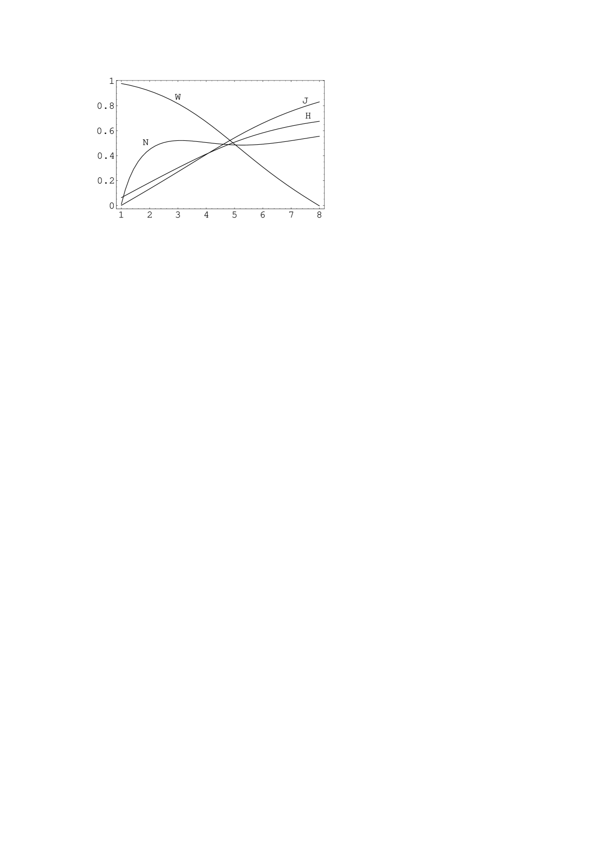
Figure 7: Black hole solution for $g=0,~{}~{}\alpha=1$ and $\beta=4$ with the horizon radius $r_{h}=.99$.

References

• [1]
• [2] R. Bartnik and J. McKinnon, Phys. Rev. Lett. 61 (1989) 141.
• [3] M. S. Volkov and D. V. Galtsov, hep-th/9810070.
• [4] M. S. Volkov and D. V. Galtsov JETP Lett. 50 (1989) 346.
• [5] H. P. Kunzle and A. K. M. Masood-ul-Alam, J. Math. Phys. 31 (1990) 928.
• [6] P. Bizon, Phys. Rev. Lett. 64 (1990) 2844.
• [7] P. Bizon and O. T. Popp, Class. Quantum Grav. 9 (1992) 193.
• [8] P. Breitenlohner, P. Forgace and D. Maison, Nucl. Phys. B 383 (1992) 357.
• [9] M. E. Ortiz, Phys. Rev. D 45 (1992) R2586.
• [10] P. Breitenlohner, P. Forgace and D. Maison, Nucl. Phys. B 442 (1995) 126.
• [11] A. Lue and E. J. Weinberg, hep-th/9905223.
• [12] G. ’t Hooft, Nucl. Phys. B 79 (1974) 276.
• [13] A. M. Polyakov, JETP Lett. 20 (1974) 194.
• [14] K. Lee, V. P. Nair and E. J. Weinberg, Phys. Rev. D 45 (1992) 2751.
• [15] P. C. Aichelburg and P. Bizon Phys. Rev. D 48 (1993) 607.
• [16] B. R. Greene, S. D. Mathur and C. M. O’Neill Phys. Rev. D 47 (1993) 2242.
• [17] Y. Brihaye, B. Hartmann and J. Kunz, Phys. Lett. B 441 (1998) 77.
• [18] Y. Brihaye, B. Hartmann, J. Kunz and N. Tell, hep-th/9904065.
• [19] K. Maeda, T. Tachizawa and T. Torii, Phys. Rev. Lett. 72 (1994) 450.
• [20] T. Torii, K. Maeda and T. Tachizawa, Phys. Rev. D 51 (1995) 1510.
• [21] T. Tachizawa, K. Maeda and T. Torii, Phys. Rev. D 51 (1995) 4054.
• [22] M. Born, Proc. R. Soc. London A 143 (1934) 410.
• [23] M. Born and M. Infeld, Proc. R. Soc. London A 144 (1934) 425.
• [24] J. Dai, R. G. Leigh and J. Polcinski, Mod. Phys. Lett. A 4 (1989) 2073
• [25] E. S. Fradkin and A. A. Tseytlin, Phys. Lett. B 163 (1985) 123.
• [26] A. A. Tseytlin, Nucl. Phys. B 276, (1986) 391.
• [27] R. G. Leigh, Mod. Phys. Lett. A 4 (1989) 2767.
• [28] C. G. Callan and J. M. Maldacena, Nucl. Phys. B 513 (1998) 198.
• [29] G. W. Gibbons, Nucl. Phys. B 514 (1998) 603.
• [30] P. S. Howe, N. D. Lambert and P. C. West, Nucl. Phys. B 515 (1998) 203.
• [31] D. Brecher, Phys. Lett. B 442 (1998) 117.
• [32] A. A. Tseytlin, Nucl. Phys. B 501 (1997) 41.
• [33] S. Gonorazky, F. A. Schaposnik and G. Silva, Phys. Lett. B 449 (1999) 187.
• [34] N. Grandi, E. F. Moreno and F. A. Schaposnik, Phys.Rev. D 59 (1999) 125014.
• [35] E.Moreno, C.Nu ez and F.A.Schaposnik, Phys.Rev. D 58 (1998) 025015.
• [36] P. K. Tripathy, Phys. Lett. B 458 (1999) 252.
• [37] P. G. Bergmann, M. Cahen and A. B. Komar, J. Math. Phys. 6 (1965) 1.
• [38] N. Grandi, R.L. Pakman, F.A.Schaposnik and G. Silva, hep-th/9906224
Refer to caption