DTP 99-47

EHU-FT/9911

hep-th/9906160

Black diholes

Roberto Emparan

Department of Mathematical Sciences
University of Durham, Durham DH1 3LE, UK
and

Departamento de Física Teórica
Universidad del País Vasco, Apdo. 644, E-48080, Bilbao, Spain

We present and analyze exact solutions of the Einstein–Maxwell and Einstein–Maxwell–Dilaton equations that describe static pairs of oppositely charged extremal black holes, i.e., black diholes. The holes are suspended in equilibrium in an external magnetic field, or held apart by cosmic strings. We comment as well on the relation of these solutions to brane–antibrane configurations in string and M-theory.

June 1999

Exact solutions of General Relativity describing multiple black holes are few and far between. Indeed one would expect such configurations to have in general a very complicated structure. Luckily, there exist some simple solutions exhibiting remarkable properties. For instance, the Majumdar–Papapetrou solutions [1] describe an arbitrary number of static extremal charged black holes, all with charges of the same sign. Equilibrium is possible due to the cancellation of the gravitational attraction against electric or magnetic repulsion. In other cases, such as in the multi-Schwarzschild solution in [2], the masses are arranged in a linear configuration, and since the gravitational attraction between them is unbalanced, conical singularities arise along the symmetry axis. Other solutions describe black holes in relative motion, such as in the cosmological multi-black hole solutions of [3], or in the C and Ernst metrics [4, 5], where two black holes accelerate apart. In this paper we want to report on a different class of solutions, which describe two static extremal magnetic black holes, this time with charges of opposite signs. The configuration therefore possesses a magnetic dipole moment, and can be appropriately called a dihole. In order to maintain the black holes in static equilibrium an external force has to be provided. This will appear in the form of a magnetic field aligned with the dihole. Otherwise, conical singularities (which may be interpreted as cosmic strings) will appear in the solution.

The diholes we will exhibit are solutions of Einstein–Maxwell theory, possibly coupled to a dilaton. The latter case includes in particular Kaluza–Klein theory, for which the dihole consists of a monopole–antimonopole pair described previously in [6]. Dipole configurations have become of recent interest also within the broader context of string and M-theory, as describing brane–antibrane configurations [7]. Near the end, we will explain that much of what we will describe below has direct relevance in that context. Other recent papers studying self–gravitating dipole solutions in string theory include [8].

The starting point in the construction of the new dihole solutions will be certain exact solutions that are known to carry magnetic dipole moment [9, 10]. We will see later that, even in the absence of an external magnetic field, these solutions admit an interpretation as dihole configurations, although conical singularities will be present in general. For simplicity of presentation, and also because it is presumably the most important case, we will study first the dihole in Einstein–Maxwell theory. The extension to dilaton theories will then be a rather straightforward task.

Several years ago [9] Bonnor constructed a solution of Einstein–Maxwell theory describing a magnetic dipole, with metric

$$ds^{2}=\left(1-{2Mr\over\Sigma}\right)^{2}\left[-dt^{2}+{\Sigma^{4}\over\left(\Delta+(M^{2}+a^{2})\sin^{2}\theta\right)^{3}}\left({dr^{2}\over\Delta}+d\theta^{2}\right)\right]+{\Delta\sin^{2}\theta\over\left(1-{2Mr\over\Sigma}\right)^{2}}d\varphi^{2}\ ,$$ (1)

and gauge potential

$$A={2aMr\sin^{2}\theta\over\Delta+a^{2}\sin^{2}\theta}\;d\varphi\ ,$$ (2)

with

$$\Delta = r^{2}-2Mr-a^{2}\ ,$$

$$\Sigma = r^{2}-a^{2}\cos^{2}\theta\ .$$ (3)

The solution is asymptotically flat, static and axially symmetric. From the asymptotic behavior of $g_{tt}$ it is easy to deduce that the mass of the solution is $2M$. The magnetic dipole moment of the solution, $\mu=2Ma$, becomes evident by examining the asymptotic form of the potential (2). Changing the sign of $a$ amounts simply to reversing the orientation of the dipole, so we will consider, without loss of generality, $a\geq 0$. For $M=0$ the solution is exactly flat. It was noticed in [9] that singularities occur at $r=r_{+}=M+\sqrt{M^{2}+a^{2}}$, where $\Delta$ vanishes. Our aim is, first, to study the structure of the singularity at $r=r_{+}$, and show that it can be removed by the introduction of an external magnetic field. Then, having the new solution with an external magnetic field, we will argue that at the endpoints of the $r=r_{+}$ line, i.e., at $(r=r_{+},\theta=0)$ and $(r=r_{+},\theta=\pi)$ lie two oppositely charged extremal Reissner-Nordström black holes, i.e., the solution describes a dihole. It will be clear then that the role played by the external magnetic field is to balance the attraction, gravitational and magnetic, between the black holes.

Let us then study the locus of $r=r_{+}$. Crucially, observe that the axial Killing vector $\partial_{\varphi}$ vanishes there. This means that $r=r_{+}$ is to be thought of as part of the symmetry axis of the solution. We are used to thinking of the lines $\theta=0,\pi$ as forming the axis of symmetry. However, in the present situation the endpoints of these two semi-axes do not come to join at a common point. Rather, the axis of symmetry is completed by the segment $r=r_{+}$. As $\theta$ varies from $0$ to $\pi$ we move along this segment from one endpoint to the other, see Fig. 1.

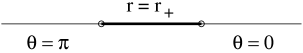
Figure 1: Axis of symmetry of the dipole solution. The lines $\theta=0,\pi$ run along $r_{+}<r<\infty$. The segment $r=r_{+}$ is parametrized by $\theta$ with range $0<\theta<\pi$.

The obvious thing to study now is whether conical singularities appear on the different portions of the symmetry axis. If $\cal C$ is the proper length of a circumference around the axis, and $\cal R$ is its proper radius, then the presence of a conical deficit $\delta$ means that $(d{\cal C}/d{\cal R})|_{{\cal R}\rightarrow 0}=2\pi-\delta$. Take $\varphi$ to be periodically identified with period $\triangle\varphi$. Then the conical deficit along the axes $\theta=0,\pi$ is

$$\delta_{(0,\pi)}=2\pi-\left|{\triangle\varphi\;d\sqrt{g_{\varphi\varphi}}\over\sqrt{g_{\theta\theta}}\;d\theta}\right|_{\theta=0,\phi}=2\pi-\triangle\varphi$$ (4)

and therefore would vanish with the standard choice $\triangle\varphi=2\pi$. However, the conical deficit along the line $r=r_{+}$,

$$\delta_{(r_{+})}=2\pi-\left|{\triangle\varphi\;d\sqrt{g_{\varphi\varphi}}\over\sqrt{g_{rr}}\;dr}\right|_{r=r_{+}}=2\pi-\left(1+{M^{2}\over a^{2}}\right)^{2}\triangle\varphi$$ (5)

does not cancel with that same choice for $\triangle\varphi$. In fact $\triangle\varphi=2\pi$ gives a conical excess. This is, there is a strut along the segment $r=r_{+}$. We can see the physical origin of the strut as providing the internal stress (pressure) needed to counterbalance the attraction between the poles.

Instead of eliminating the conical defect outside the dipole, the period $\triangle\varphi$ can be chosen to cancel the singularity along $r=r_{+}$. With such a choice one finds a conical deficit running along the axes $\theta=0,\pi$, from the endpoints of the dipole to infinity. We can view such defects as “cosmic strings,” with tension

$$T={\delta_{(0,\pi)}\over 8\pi}={1\over 4}\left[1-\left({a^{2}\over M^{2}+a^{2}}\right)^{2}\right]\ .$$ (6)

The dipole is then suspended by open cosmic strings that pull from its endpoints. The line $r=r_{+}$, $0<\theta<\pi$, joining these is now completely non-singular.

Although the proper length of the segment $r=r_{+}$, $0\leq\theta\leq\pi$ is infinite, the parameter $a$ gives, in a sense, an indication of the separation between the poles. For large values of $a$ the force required to keep the dipole static becomes $T\rightarrow{M^{2}\over 2a^{2}}$, which decreases as $a^{-2}$ as expected from a Newtonian approximation to the attraction between poles. Notice however that in the limit $a\rightarrow 0$ the tension tends to a finite limit $T\rightarrow 1/4$. In this limit the magnetic dipole moment of the solution vanishes but nevertheless one does not recover the Schwarzschild solution. Rather, a nakedly singular solution appears, with higher mass–multipoles [9].

The recourse to cosmic strings to account for the conical singularities of the metric might appear as a rather ad hoc prescription. From a physical standpoint it appears that an external magnetic field aligned with the dipole should be able to provide the necessary force to balance the attraction between the poles, by pulling apart the dipole endpoints. By adequately tuning the magnetic field, the stresses along the axis should be made to disappear.

It is indeed possible to introduce such a magnetic field by means of a Harrison transformation [11] on the solution. In doing so we proceed in a manner entirely analogous to Ernst’s elimination of the conical singularities of the C-metric [5]. The Harrison transformation of Einstein-Maxwell theory takes an axisymmetric solution to another solution containing a magnetic field that asymptotes to the Melvin magnetic universe [12]. This is a flux tube that provides the best possible approximation to a uniform magnetic field in General Relativity.

For an axisymmetric solution of the Einstein-Maxwell theory with $g_{i\varphi}=A_{i}=0$ for $i\neq\varphi$, the Harrison transformation acts as

$$g^{\prime}_{ij} = \lambda^{2}g_{ij}\quad{\rm for}\;\;i,j\neq\varphi\ ,\qquad g^{\prime}_{\varphi\varphi}=\lambda^{-2}g_{\varphi\varphi}\ ,$$

$$A^{\prime}_{\varphi} = {2\over\lambda B}\left(1+{BA_{\varphi}\over 2}\right)+k\ ,$$

$$\lambda = \left(1+{BA_{\varphi}\over 2}\right)^{2}+{B^{2}\over 4}g_{\varphi\varphi}\ ,$$ (7)

where $k$ is an arbitrary constant that can be chosen so as to remove Dirac strings.

We apply now this transformation to the Bonnor solution, eqs. (1) and (2), and obtain, after some algebra, and choosing $k=-2/B$,

$$ds^{2}=\Lambda^{2}\left[-dt^{2}+{\Sigma^{4}\over\left(\Delta+(M^{2}+a^{2})\sin^{2}\theta\right)^{3}}\left({dr^{2}\over\Delta}+d\theta^{2}\right)\right]+{\Delta\sin^{2}\theta\over\Lambda^{2}}d\varphi^{2}\ ,$$ (8)

and

$$A_{\varphi}=-{2Mra+{1\over 2}B[(r^{2}-a^{2})^{2}+\Delta a^{2}\sin^{2}\theta]\over\Lambda\Sigma}\sin^{2}\theta\ ,$$ (9)

where $\Delta$ and $\Sigma$ are as in (3) and

$$\Lambda={\Delta+a^{2}\sin^{2}\theta+2BMra\sin^{2}\theta+{1\over 4}B^{2}\sin^{2}\theta[(r^{2}-a^{2})^{2}+\Delta a^{2}\sin^{2}\theta]\over\Sigma}\ .$$ (10)

It is straightforward to see that as $r\rightarrow\infty$ the solution approaches the same limit as the Melvin universe with axial magnetic field $B$. Let us investigate now the conical structure along the symmetry axis. Along the outer semi-axes, $\theta=0,\pi$, we find the same value for the conical defect as in (4), so, in order to set $\delta_{(0,\pi)}=0$, we will choose $\triangle\varphi=2\pi$. On the other hand, along the inner segment of the axis, $r=r_{+}$, we find now

$$\delta_{(r_{+})}=2\pi-\left(1+{M^{2}\over a^{2}}\right)^{2}\left(1+{BMr_{+}\over a}\right)^{-4}\triangle\varphi\ ,$$ (11)

and with the choice $\triangle\varphi=2\pi$ we see that the conical defect can be cancelled if the magnetic field is chosen to be

$$B={\pm\sqrt{M^{2}+a^{2}}-a\over Mr_{+}}=\pm{2M\over(r_{+}\pm a)^{2}}\ .$$ (12)

There are two branches of solutions, one with $B>0$ and another one with $B<0$ (recall that we are taking $a\geq 0$). For the first branch, in the limit $a\rightarrow\infty$ the field goes to zero like $B\rightarrow{M\over 2a^{2}}$, whereas for $a\rightarrow 0$ the field tends to a non-zero value $B\rightarrow 1/(2M)$. In the second branch $B\rightarrow-2/M$ as $a\rightarrow\infty$. An analogous branch structure was found in [13] for the Ernst metric, where the second branch was found to be somewhat anomalous. We will not discuss that here, and in the following we will only consider the first branch of solutions (upper signs) in (12). Observe that values of $B$ larger than (12) would have yielded a cosmic string stretching along the dipole, a “dumbbell” configuration similar to that considered in [14].

We have therefore succeeded in removing the conical singularities of the Bonnor dipole solution. However, the metric still becomes singular at the endpoints of the dipole, $(r=r_{+},\theta=0)$ and $(r=r_{+},\theta=\pi)$. Remarkably, we can show that these singularities are merely artifacts of the coordinate system. In order to do so, let us study the geometry of the region very close to these points. To this effect, change the coordinates $(r,\theta)$ to $(\rho,{\bar{\theta}})$ as

$$r = r_{+}+{\rho\over 2}(1+\cos{\bar{\theta}})\ ,$$

$$\sin^{2}\theta = {1\over\sqrt{M^{2}+a^{2}}}\rho(1-\cos{\bar{\theta}})\ ,$$ (13)

and take $\rho$ to be much smaller than any other length scale involved so as to get near the poles. In this limit the solution becomes, near $(r=r_{+},\theta=0)$,

$$ds^{2}=-{\rho^{2}\over Q^{2}}dt^{2}+{Q^{2}\over\rho^{2}}d\rho^{2}+Q^{2}(d{\bar{\theta}}^{2}+\sin^{2}{\bar{\theta}}d\varphi^{2})\ ,$$ (14)

$$A_{\varphi}=-Q(1-\cos{\bar{\theta}})\ ,$$ (15)

where

$$Q={Mr_{+}\over\sqrt{M^{2}+a^{2}}}\ .$$ (16)

This is precisely the Bertotti–Robinson solution, AdS${}_{2}\times S^{2}$, which describes the near horizon limit of an extreme Reissner–Nordström black hole with charge $-Q$. In a similar way, at the other endpoint $(r=r_{+},\theta=\pi)$ we find the same geometry but this time with the opposite charge. Therefore, the solution contains regular horizons at the poles, and it can be continued beyond $\rho=0$.

Apparently, the field $B$ has no effect down the throat (14). But, crucially, realize that in order to arrive at (14) the field $B$ is required to take precisely the value (12). It is illuminating to see how things change for other values of $B$. If we keep $B$ arbitrary, then the limiting form of the solution near the poles is

$$ds^{2}=g^{2}({\bar{\theta}})\left[-{\rho^{2}\over Q^{2}}dt^{2}+{Q^{2}\over\rho^{2}}d\rho^{2}+Q^{2}d{\bar{\theta}}^{2}\right]+{Q^{2}\sin^{2}{\bar{\theta}}\over g^{2}({\bar{\theta}})}d\varphi^{2}\ ,$$ (17)

with $Q$ as in (16) above, and where

$$g({\bar{\theta}})={1\over 2}\left[1+\cos{\bar{\theta}}+\left({a\over\sqrt{M^{2}+a^{2}}}+BQ\right)^{2}(1-\cos{\bar{\theta}})\right]$$ (18)

is a function such that $g({\bar{\theta}})=1$ when the field $B$ is tuned to the value (12). The important point is that in general the surface $\rho=0$ is still a horizon, albeit not one of spherical symmetry. Instead, the horizon is a prolate spheroid, which is further distorted by a conical defect at either pole. We want to stress that the horizons are present even for the case of the Bonnor dipole ($B=0$). As far as we know, this crucial feature of the Bonnor solution (1) has gone unnoticed in all previous literature.

The gauge field near the horizon is also distorted from its monopolar form to

$$A_{\varphi}=-Q\left({a\over\sqrt{M^{2}+a^{2}}}+BQ\right){1-\cos{\bar{\theta}}\over g({\bar{\theta}})}\ .$$ (19)

The physical magnetic charge of the hole can now be computed using Gauss’s law, $\hat{Q}={1\over 4\pi}\int_{S^{2}}F$ ($S^{2}$ is any topological sphere surrounding the charge) so, in general, the actual physical charge of the hole is not $Q$, but rather

$$\hat{Q}={\triangle\varphi\over 4\pi}\left(A_{\varphi}({\bar{\theta}}=\pi)-A_{\varphi}({\bar{\theta}}=0)\right)={\triangle\varphi\over 2\pi}{Q\over{a\over\sqrt{M^{2}+a^{2}}}+BQ}\ .$$ (20)

The limiting geometries above were valid for arbitrary values of $a$, as long as we remain close enough to the pole. If, instead, we consider the limit of very large $a$, while keeping $r-r_{+}$ and $a\sin^{2}\theta$ finite, the solution (8) tends to

$$ds^{2}=-\left(1+{Q\over\rho}\right)^{-2}dt^{2}+\left(1+{Q\over\rho}\right)^{2}[d\rho^{2}+\rho^{2}(d{\bar{\theta}}^{2}+\sin^{2}{\bar{\theta}}d\varphi^{2})]\ ,$$ (21)

with $Q\rightarrow M$, and $A_{\varphi}$ as in (15). We recognize this as the extremal Reissner–Nordström black hole. In the limit $a\rightarrow\infty$ the magnetic field $B$ vanishes, consistently with the interpretation that the poles are “infinitely apart” from each other and the force between them goes to zero. Incidentally, note that if one wanted to consider an adiabatic process where the two black holes held in equilibrium are taken apart, then the magnetic field would obviously have to be adjusted at every moment in such a way that the field precisely balances the forces for fixed values of the charge of each hole (20).

So we conclude that our solution (8), (9) indeed describes a dihole. In general, for finite values of $a$, the geometry of the black holes is distorted from their asymptotically flat form (21), but, for the particular value of $B$ in (12), the distortion becomes inappreciable well down the throat, where we recover the near horizon geometry (14). Moreover, the infinite proper distance along the dipole line $r=r_{+}$ is now seen as a consequence of the infinite throat characteristic of extremal Reissner–Nordström black holes.

The dihole character of the dipole solution brings about some interesting consequences (now we restrict ourselves to the solution with $B$ given by the upper sign solution in (12)). There is a non–vanishing area associated to the horizon of each of the black holes, and therefore an entropy. This is easily obtained from (14) as $S={\cal A}_{h}/4=\pi Q^{2}$ for each hole.

In the limit of large separation between the holes we would expect a Newtonian approximation to become reasonable. Indeed, for large $a$, the magnetic field $B$ exerts the right force, $T\approx QB\approx Q^{2}/(2a^{2})$ to counterbalance the attraction between two particles at a distance of the order of $a$.

As $a\rightarrow 0$, though, there is the peculiarity that the black holes in (8) never appear to merge. For $a=0$ the solution is non–singular (outside the horizons), and is to be interpreted as the configuration of minimal separation between the black holes. It corresponds to a maximum value for $QB$, namely $(QB)_{\rm max}=1$.

We have mentioned that the mass of the dipole was, for Bonnor’s asymptotically flat solution, equal to $2M$. The solution (8), (9) is instead asymptotic to the Melvin universe, but it is still possible to compute its energy by taking the Melvin universe as the reference background, following [15]. The result is that the energy is still equal to $2M$. In the limit of large separation the mass of each black hole (21) is $M$, so the total energy is the sum of the energies of the separate black holes. Thus, for infinite separation the interaction energy vanishes, as could have been expected.

Now, at finite values of $a$ we would expect to find a non–vanishing interaction energy. Given that extremal black holes in isolation satisfy $M_{\rm bh}=Q$, we can estimate the interaction energy in the dipole as

$$E_{\rm int}=E_{\rm total}-2M_{\rm bh}=2M-2Q=-{2M^{2}\over\sqrt{M^{2}+a^{2}}}\ .$$ (22)

This is negative, reflecting the attraction between the black holes. For fixed black hole charge $Q$, this energy is minimized when $a=0$. Notice that the value as $a\rightarrow 0$ is $E_{\rm int}=-2M$.

Now let us turn to the generalization of these diholes to theories with a dilaton field $\phi$. The action we consider is

$$I={1\over 16\pi G}\int d^{4}x\;\sqrt{-g}\left(R-2(\partial\phi)^{2}-e^{-2\alpha\phi}F^{2}\right)\ .$$ (23)

For dilaton coupling $\alpha=0$ we will recover the results discussed above. The case of $\alpha^{2}=3$ corresponds to Kaluza–Klein theory, and in this case the solutions admit nice geometric interpretations. The Kaluza–Klein analog of the Bonnor dipole was identified in [16]. The introduction of the background magnetic field, together with a thorough analysis of the structure of the solutions and extensions to higher dimensions, was undertaken in [6].

For arbitrary values of the dilaton coupling, the counterparts of the Bonnor dipole were obtained in [10]. The conical singularity along the axis was correctly identified there. Indeed, a straightforward calculation like the one in (5) shows that the conical deficit is present for arbitrary values of $\alpha$. More importantly, we will find that the entire dihole structure reveals itself for any value of $\alpha$, in a manner entirely analogous to the Einstein–Maxwell dihole. This is at variance with the conclusions in [10], an issue we will return to below, after completing our analysis.

It is a straightforward matter to take the dipole solutions in [10] and subject them to a dilatonic Harrison transformation [17]. The resulting metric is

$$ds^{2}=\Lambda^{2\over 1+\alpha^{2}}\left[-dt^{2}+{\Sigma^{4\over 1+\alpha^{2}}\over\left(\Delta+(M^{2}+a^{2})\sin^{2}\theta\right)^{3-\alpha^{2}\over 1+\alpha^{2}}}\left({dr^{2}\over\Delta}+d\theta^{2}\right)\right]+{\Delta\sin^{2}\theta\over\Lambda^{2\over 1+\alpha^{2}}}d\varphi^{2}\ ,$$ (24)

the dilaton, $e^{-\phi}=\Lambda^{\alpha\over 1+\alpha^{2}}$, and the gauge potential,

$$A_{\varphi}=-{{2\over\sqrt{1+\alpha^{2}}}Mra+{1\over 2}B[(r^{2}-a^{2})^{2}+\Delta a^{2}\sin^{2}\theta]\over\Lambda\Sigma}\sin^{2}\theta\ ,$$ (25)

with

$$\Lambda={\Delta+a^{2}\sin^{2}\theta+2\sqrt{1+\alpha^{2}}BMra\sin^{2}\theta+{1+\alpha^{2}\over 4}B^{2}\sin^{2}\theta[(r^{2}-a^{2})^{2}+\Delta a^{2}\sin^{2}\theta]\over\Sigma}\ .$$ (26)

and $\Delta$ and $\Sigma$ still given by (3).

The analysis of these solutions can be carried out in the same manner as above for the Einstein–Maxwell dihole, only in this case at the poles we find extremal dilatonic holes, the horizons being replaced by null singularities. The solutions asymptote to the dilaton Melvin solutions of [18]. The value of the magnetic field that removes all conical singularities is

$$B={2\over\sqrt{1+\alpha^{2}}}{M\over(r_{+}+a)^{2}}$$ (27)

(a second branch also exists for these cases). The same coordinate change as in eq. (13) yields, for large $a$,

$$ds^{2}=-\left(1+{Q\over\rho}\right)^{-{2\over 1+\alpha^{2}}}dt^{2}+\left(1+{Q\over\rho}\right)^{2\over 1+\alpha^{2}}[d\rho^{2}+\rho^{2}(d{\bar{\theta}}^{2}+\sin^{2}{\bar{\theta}}d\varphi^{2})]\ ,$$ (28)

with a monopole potential $A_{\varphi}$ of charge $Q/\sqrt{1+\alpha^{2}}$, and dilaton $e^{\phi}=\left(1+{Q\over\rho}\right)^{\alpha\over 1+\alpha^{2}}$. These solutions are the extremal dilatonic holes of [18].

In the same manner as we have done before in the absence of dilaton, we can also keep $a$ finite, but go to small values of $\rho$. In this way we recover the geometry near the (singular) horizon $\rho=0$ of the extreme dilatonic hole, with the parameter $Q$ defined as in (16), and some angular distortion when $B$ takes values different from (27). This is,

$$ds^{2}\rightarrow g({\bar{\theta}})^{2\over 1+\alpha^{2}}\left[-\left({\rho\over Q}\right)^{2\over 1+\alpha^{2}}dt^{2}+\left({Q\over\rho}\right)^{2\over 1+\alpha^{2}}\left(d\rho^{2}+\rho^{2}d{\bar{\theta}}^{2}\right)\right]+\left({Q\over\rho}\right)^{2\over 1+\alpha^{2}}{\rho^{2}\sin^{2}{\bar{\theta}}\over g({\bar{\theta}})^{2\over 1+\alpha^{2}}d\varphi^{2}}\ ,$$ (29)

now with

$$g({\bar{\theta}})={1\over 2}\left[1+\cos{\bar{\theta}}+\left({a\over\sqrt{M^{2}+a^{2}}}+BQ\sqrt{1+\alpha^{2}}\right)^{2}(1-\cos{\bar{\theta}})\right]\ .$$ (30)

In these coordinates it is easy to compute the scalar curvature near the poles $r=r_{+}$, $\theta=0,\pi$ since these loci correspond to $\rho=0$. One finds

$$R\rightarrow{f({\bar{\theta}})\over\rho^{2\alpha^{2}\over 1+\alpha^{2}}}\ ,$$ (31)

where $f({\bar{\theta}})$ is a certain function which is regular for $0\leq{\bar{\theta}}\leq\pi$. We can see that the scalar curvature diverges at $\rho=0$ except when $\alpha=0$. Thus $\rho=0$ (i.e., $r=r_{+},\theta=0,\pi$) is, for $\alpha\neq 0$, a real singularity. But this is just the well-known null singularity of extremal dilatonic holes. These holes do not have any Bekenstein–Hawking entropy associated. The proper distance between the holes for $\alpha\neq 0$ is finite, since in that case the proper distance to the (singular) horizon of each hole (28) is known to be finite. Besides, for values of $B$ other than (27) the geometry around the singular horizon is angularly deformed in a manner similar to (17).

A very different interpretation of the geometry was proposed in [10], where it was claimed that for $\alpha=1$ (and only for that value) regular non-extremal horizons are present at the poles $r=r_{+}$, $\theta=0,\pi$. The analysis of [10] was based on a study of certain two-dimensional sections of the solution, in particular of the geometry of the two-dimensional section given by $r=r_{+}$, $\varphi={\rm constant}$. It was pointed out in that paper that the intrinsic curvature of this two-dimensional metric is divergent at $\theta=0,\pi$ unless $\alpha=1$. However, such a restricted two-dimensional study cannot be conclusive, if only for the fact that singularities of a submanifold do not in general correspond to singularities of the full manifold. The analysis is indeed misleading: The full four-dimensional structure of the solutions near the poles is manifested using the coordinates ($t$, $\rho$, ${\bar{\theta}}$, $\varphi$) as introduced in (13), and then eq. (31) explictly shows that only $\alpha=0$ yields a non-singular four-dimensional curvature at $\rho=0$. This is just as expected from the fact that we have recovered the geometries near the horizon of extremal charged dilatonic black holes, of which only the pure Einstein-Maxwell case possesses a regular horizon. The standard analysis of the structure near the horizon of the extremal Reissner-Nordstrom black hole and its limiting Bertotti-Robinson geometry can be equally well applied to (14). In particular, future directed geodesics can cross each of the horizons at each pole, so at both poles we have future horizons. Since the geometry is symmetric under time-reversal there are also past horizons. Also, the coordinates can be extended in the standard manner beyond the horizons. This forms the basis of our claim that the non-dilatonic solution describes a time-symmetric configuration with two extremal black holes, each with a future and a past horizon. This is obviously at variance with the claim in [10] of a non-extremal white hole (a past horizon) at one pole and a black hole (a future horizon) at the other pole for $\alpha=1$ (and a singularity for $\alpha\neq 1$). Actually, this time-asymmetric interpretation is another artifact of the restriction to the two-dimensional submanifold mentioned above. We would also like to stress that our interpretation is in consonance with the one given in [6] for the case $\alpha=\sqrt{3}$, and extends it in a natural way to other values of $\alpha$.

Let us now discuss some generic aspects of the dihole solutions we have constructed. First of all, we have shown that the solutions of [9] and [10] are properly interpreted, for arbitrary values of the dilaton coupling, as diholes, with the holes being kept in equilibrium by strings or struts. The horizon of each hole is deformed by the field created by the other hole, as well as by the conical defect. We have found that an external field can be applied and tuned so as to balance the system and remove the conical singularities. In that case, the external field precisely cancels the field created by the other hole, with the effect that the distortion disappears and the horizon is spherically symmetric.

On the other hand, the conical defects that pull apart the holes in the Bonnor dihole can be made more physical by regarding them as the limit of self–gravitating vortices that end on the black holes. Therefore they add to the catalog of solutions describing cosmic strings ending on black holes [20, 14].

Another aspect to note is that the configurations are expected to be unstable. On physical grounds it is clear that a slight deviation from the equilibrium configuration should set the black holes either in runaway motion away from each other, or collapsing onto one another. As a matter of fact, the instability of the dihole is known to be present for the $a=0$ solution in the Kaluza–Klein case $\alpha=\sqrt{3}$. In that case the solution can be related to the Euclidean Schwarzschild instanton, which is known to have an unstable mode [21].

Indeed, the instability of these solutions fits in nicely with the existence of instantons describing the pair creation of black holes in an external field [19] or in the breaking of a cosmic string [20]. The diholes are to be seen as the sphalerons sitting on top of the potential barrier, under which the tunneling process takes place. Thus, the dihole solutions in this paper are closely linked to the C and Ernst type of solutions that describe black holes accelerating apart [4, 5, 17].

We have mentioned as well that, when held in the external field, it does not appear to be possible to bring the black holes close enough to make them merge. Fixing the charge, there is an upper limiting value for the magnetic field, which is approached as $a\rightarrow 0$ for the branch with $B>0$. In this limit the two-black hole structure still persists. This might be seen as providing support for the cosmic censorship conjecture: the merging of the Reissner–Nordström black holes, which would imply the annihilation of charge and possibly a change in the spatial topology, might have led to a naked singularity. Nevertheless, notice that for the Bonnor dihole kept in equilibrium by cosmic strings, the black holes actually merge as $a\rightarrow 0$, and then form a singularity. However, these “tests” must be taken with a pinch of salt, since given the instability of the solutions, a gedanken experiment in which the black holes are slowly moved towards one another does not appear to be physically realizable. Related analyses of cosmic censorship can be found in [13].

Several extensions of the work presented in this paper seem possible. First of all, it is clear that electric diholes can be constructed simply by dualizing the magnetic field to an electric field. More interesting are generalizations to theories with a richer field content. Dilaton black holes with coupling $\alpha=0,1/\sqrt{3},1,\sqrt{3}$ are known to occur in the low energy description of string and M-theory compactified down to four dimensions. They admit an interpretation in terms of branes intersecting in higher dimensions, with all the longitudinal and relative transverse coordinates being compactified. As one example among many possible embeddings, the Reissner–Nordström black hole can be obtained as an intersection of e.g., four equally charged D3-branes [22]. We can lift our solution (8) to ten dimensions by suitably adding flat dimensions, and then interpret it as an intersecting brane-antibrane configuration. A similar lift can also be done for the solutions with the other three special values of $\alpha$.

Now, when the charges of the branes are not equal to one another, the four dimensional black holes appear as solutions to theories with four $U(1)$ gauge fields and three independent scalars [23]. It is likely that dihole solutions for these theories can be constructed. Indeed, the existence of C and Ernst–type metrics in such $U(1)^{4}$ theories, describing pairs of black holes accelerating apart [24] strongly suggests that it should be possible to construct their static dihole counterparts.

On the other hand, it is less clear how to obtain non-extreme diholes. Also, one might speculate on the possibility that the dihole be held in equilibrium not by an external magnetic field, but rather by the expansion produced by a positive cosmological constant. To our knowledge, such solutions have not been constructed yet.

References

- [1] S.D. Majumdar, Phys. Rev. 72, 390 (1947); A. Papapetrou, Proc. Roy. Irish. Acad. A51, 191 (1947).
- [2] W. Israel and K.A. Khan, Nuovo Cim. 33, 331 (1964).
- [3] D. Kastor and J. Traschen, Phys. Rev. D47, 5370 (1993) hep-th/9212035.
- [4] W. Kinnersley and M. Walker, Phys. Rev. D2, 1359 (1970).
- [5] F.J. Ernst, J. Math. Phys. 17 515 (1976).
- [6] F. Dowker, J.P. Gauntlett, G.W. Gibbons and G.T. Horowitz, Phys. Rev. D53, 7115 (1996) hep-th/9512154.
- [7] A. Sen, JHEP 10, 002 (1997) hep-th/9708002.
- [8] S. Mukherji, hep-th/9903012; B. Janssen and S. Mukherji, hep-th/9905153.
- [9] W.B. Bonnor, Z. Phys. 190, 444 (1966).
- [10] A. Davidson and E. Gedalin, Phys. Lett. B339, 304 (1994) gr-qc/9408006.
- [11] B.K. Harrison, J. Math. Phys. 9 1744 (1968).
- [12] M.A. Melvin, Phys. Lett. 8, 65 (1964).
- [13] G.T. Horowitz and H.J. Sheinblatt, Phys. Rev. D55, 650 (1997) gr-qc/9607027.
- [14] R. Emparan, Phys. Rev. Lett. 75, 3386 (1995) gr-qc/9506025.
- [15] S.W. Hawking and G.T. Horowitz, Class. Quant. Grav. 13, 1487 (1996) gr-qc/9501014.
- [16] D.J. Gross and M.J. Perry, Nucl. Phys. B226, 29 (1983).
- [17] F. Dowker, J.P. Gauntlett, D.A. Kastor and J. Traschen, Phys. Rev. D49, 2909 (1994) hep-th/9309075.
- [18] G.W. Gibbons and K. Maeda, Nucl. Phys. B298, 741 (1988).
- [19] D. Garfinkle and A. Strominger, Phys. Lett. B256, 146 (1991); D. Garfinkle, S.B. Giddings and A. Strominger, Phys. Rev. D49, 958 (1994) gr-qc/9306023.
- [20] M. Aryal, L.H. Ford and A. Vilenkin, Phys. Rev. D34, 2263 (1986); A. Achucarro, R. Gregory and K. Kuijken, Phys. Rev. D52, 5729 (1995) gr-qc/9505039; S.W. Hawking and S.F. Ross, Phys. Rev. Lett. 75, 3382 (1995) gr-qc/9506020; D.M. Eardley, G.T. Horowitz, D.A. Kastor and J. Traschen, Phys. Rev. Lett. 75, 3390 (1995) gr-qc/9506041; R. Gregory and M. Hindmarsh, Phys. Rev. D52, 5598 (1995) gr-qc/9506054; R. Emparan, Phys. Rev. D52, 6976 (1995) gr-qc/9507002.
- [21] D.J. Gross, M.J. Perry and L.G. Yaffe, Phys. Rev. D25, 330 (1982).
- [22] V. Balasubramanian and F. Larsen, Nucl. Phys. B478, 199 (1996) hep-th/9604189.
- [23] M. Cvetič and D. Youm, Phys. Rev. D53, 584 (1996) hep-th/9507090.
- [24] R. Emparan, Phys. Lett. B387, 721 (1996) hep-th/9607102; R. Emparan, Nucl. Phys. B490, 365 (1997) hep-th/9610170.
- [25] T. Ortín, Phys. Rev. Lett. 76, 3890 (1996) hep-th/9602067.