Effective Supergravity from Heterotic M–Theory and its Phenomenological Implications

Abstract:

In this talk I summarize several recent results concerning the four–dimensional effective supergravity obtained using a Calabi–Yau compactification of the $E_{8}\times E_{8}$ heterotic string from M–theory. A simple macroscopic study is provided expanding the theory in powers of two dimensionless variables. Higher order terms in the Kähler potential are identified and matched with the heterotic string corrections. In the context of this M–theory expansion, I discuss several phenomenological issues: universality of soft scalar masses, relations between the different scales of the theory (eleven–dimensional Planck mass, compactification scale and orbifold scale) in order to obtain unification at $3\times 10^{16}$ GeV or lower values, soft supersymmetry–breaking terms, and finally charge and colour breaking minima. The above analyses are also carried out in the presence of (non–perturbative) five–branes.

F FTUAM 99/19
IFT-UAM/CSIC-99-24
June 1999

1 Introduction and summary

One of the most exciting proposals of the last years in string theory, consists of the possibility that the five distinct superstring theories in ten dimensions plus supergravity in eleven dimensions be different vacua in the moduli space of a single underlying eleven–dimensional theory, the so–called M–theory [1]. In this respect, Hořava and Witten proposed that the strong–coupling limit of $E_{8}\times E_{8}$ heterotic string theory can be obtained from M–theory. They used the low–energy limit of M–theory, eleven-dimensional supergravity, on a manifold with boundary (a $S^{1}/Z_{2}$ orbifold), with the $E_{8}$ gauge multiplets at each of the two ten–dimensional boundaries (the orbifold fixed planes) [2].

In the present paper I will summarize several recent results concerning the four–dimensional implications of this so called heterotic M–theory. In particular, I will concentrate on the analysis of the effective supergravity obtained by compactifying heterotic M–theory on a six–dimensional Calabi–Yau manifold and its phenomenological consequences.

The effective action of this limit has been systematically analyzed in an expansion in powers of $\kappa^{2/3}$, where $\kappa^{2}$ denotes the eleven–dimensional gravitational coupling [3]. As was noticed in [4], this leads to an expansion parameter which scales as $\kappa^{2/3}\rho/V^{2/3}$, where $\pi\rho$ denotes the length of the eleventh segment and $V$ is the Calabi–Yau volume. At the leading order in this expansion, the Kähler potential, superpotential and gauge kinetic functions have been computed in [4, 5, 6, 7]. It is rather easy to determine the order $\epsilon_{1}$ correction to the leading order gauge kinetic functions [4, 8, 7, 9], while it is much more nontrivial to compute the order $\epsilon_{1}$ correction to the leading order Kähler potential, which was recently done by Lukas, Ovrut and Waldram [10]. It was argued in [11] that the holomorphy and Peccei–Quinn symmetries guarantee that there is no further correction to the gauge kinetic functions and the superpotential at any finite order in the M–theory expansion, similarly to the case of the perturbative heterotic string [12].

On the other hand, as is well known, the four–dimensional effective action of the weakly coupled heterotic string theory can be expanded in powers of the two dimensionless variables: the string coupling $\epsilon_{s}=e^{2\phi}/(2\pi)^{5}$ and the worldsheet sigma–model coupling $\epsilon_{\sigma}=4\pi\alpha^{\prime}/V^{1/3}$. It was suggested in [11] that the effective action of M-theory can be similarly analyzed by expanding it in powers of the two dimensionless variables: $\epsilon_{1}=\kappa^{2/3}\pi\rho/V^{2/3}$ and $\epsilon_{2}=\kappa^{2/3}/\pi\rho V^{1/3}$. The latter is the straightforward generalization of the string world–sheet coupling $\sim\alpha^{\prime}/V^{1/3}$ to the membrane world–volume coupling $\sim\kappa^{2/3}/\rho V^{1/3}$ since $\kappa^{2/3}$ may be identified as the inverse of the membrane tension. Note that in the M–theory limit, heterotic string corresponds to a membrane stretched along the eleventh dimension. In this framework the Kähler potential is expected to receive corrections which are higher order in $\epsilon_{1}$ or $\epsilon_{2}$. An explicit computation of these higher order corrections will be highly nontrivial since first of all the eleven–dimensional action is known only up to the terms of order $\kappa^{2/3}$ relative to the zeroth order action (except for the order $\kappa^{4/3}$ four-gaugino term) and secondly the higher order computation of the compactification solution and its Kaluza-Klein reduction are much more complicated.

In section 2, we will provide a simple macroscopic analysis of the four–dimensional effective supergravity action by expanding it in powers of $\epsilon_{1}$ and $\epsilon_{2}$. Possible higher order corrections in the Kähler potential are identified and matched with the heterotic string corrections, and their size is estimated for the physically interesting values of moduli [11]. The validity of this procedure has been explicitly checked in [15] in the case of M–theory compactified on $S^{1}/Z_{2}\times K3\times T^{2}$.

On the other hand, we will also discuss in detail how these effective supergravity models can be strongly constrained by imposing the phenomenological requirement of universal soft scalar masses, in order to avoid dangerous flavour changing neutral current phenomena. As pointed out in [13], there is a simple solution to avoid this problem: to work with Calabi–Yau spaces with one Kähler modulus $T$ only. Of course, the existence of such spaces, as e.g. the quintic hypersurface in $CP^{4}$, and their universality properties was also known in the context of the weakly–coupled heterotic string, however the novel fact in heterotic M–theory, is that model building is relatively easy. For example, in the presence of non–standard embedding and five–branes (non–perturbative objects located at points throughout the orbifold interval [3]) to obtain three–generation models with realistic gauge groups, as for example $SU(5)$, is not specially difficult [14].

Other phenomenological implications of heterotic M–theory, turn out to be also advantageous with respect to the ones of the perturbative heterotic–string theory. First of all, the resulting four–dimensional effective theory can reconcile the observed Planck scale $M_{Planck}=1.2\times 10^{19}$ GeV with the phenomenologically favored GUT scale $M_{GUT}\approx 3\times 10^{16}$ GeV in a natural manner, providing an attractive framework for the unification of couplings [3, 4]. This is to be compared to the weakly–coupled heterotic string where $M_{string}\approx 8.5\times 10^{17}$ GeV. Another phenomenological virtue of the M–theory limit is that there can be a QCD axion whose high energy axion potential is suppressed enough so that the strong CP problem can be solved by the axion mechanism [4, 8]. About the issue of supersymmetry breaking, the possibility of generating it by the gaugino condensation on the hidden boundary has been studied [16, 7, 17, 18, 19, 20] and also some interesting features of the resulting soft supersymmetry–breaking terms were discussed. In particular, gaugino masses turn out to be of the same order as squark masses [7]. This is welcome since gaugino masses much smaller than squark masses, as in the weakly–coupled heterotic string case, may give rise to a hierarchy problem [21]. For example, the experimental lower bound on gluino masses of $150$ GeV would imply scalar masses larger than $1$ TeV. Besides, the phenomenologically favored vacuum expectation values of the moduli can be obtained with several gaugino condensates with the appropriate hidden matter [20], similarly to the case of the weakly–coupled heterotic string [22]. However, it is fair to say that unlike the latter non–perturbative membrane instantons are also necessary in M–theory to obtain the desired minimum.

Several of the above mentioned phenomenological issues will be analyzed in the next sections. In section 3 we will concentrate in the case of standard and non–standard embedding vacua [23, 24, 25, 26], whereas in section 4 vacua in the presence of five–branes [26, 13] are studied. The latter are characterized basically by new moduli $Z_{n}$ associated with the five–brane positions in the orbifold dimension. In both cases we will perform a detailed study of the different scales of the theory, as well as a systematic analysis of the soft supersymmetry–breaking terms.

Concerning the former, the relations between the eleven–dimensional Planck mass, the Calabi–Yau compactification scale and the orbifold scale, taking into account higher order corrections to the leading order formulae, will be analyzed [27]. Identifying the compactification scale with the GUT scale, to obtain $M_{GUT}\approx 3\times 10^{16}$ GeV is simpler in non–standard embedding models than in standard ones. In the presence of five–branes, $M_{GUT}$ can be obtained more easily. On the other hand, going away from perturbative vacua, it was recently realized that the string scale may be anywhere between the weak scale and the Planck scale [28] and the size of the extra dimensions may be as large as a millimetre [29]. Whether or not all these scenarios are possible in the context of heterotic M–theory has been analyzed recently in [30] with interesting results: to lower the unification scale (and therefore the eleven–dimensional Planck scale which is around two times bigger) to intermediate values $\approx 10^{11}$ GeV or $1$ TeV values or to obtain the radius of the orbifold as large as a millimetre is in principle possible in some special limits. However, it has been pointed out in [27] that the necessity of a fine–tuning or the existence of a hierarchy problem renders these possibilities unnatural. Although new possibilities arise in the presence of five–branes in order to lower the scales, again at the cost of introducing a huge hierarchy problem.

We will also analyze the soft supersymmetry breaking terms under the general assumption that supersymmetry is spontaneously broken by the auxiliary components of the bulk moduli superfields (dilaton $S$ and modulus $T$) [11, 18, 31, 27]. It is examined in particular how the soft terms vary when one moves from the weakly–coupled heterotic string limit to the strongly–coupled limit. The presence of new parameters in the formulae gives rise to different pattern of soft terms. This is also the case of models with five–branes where at least a new goldstino angle, associated to a modulus $Z_{1}$, must be included in the computation [13, 32, 27]. Unlike the weakly–coupled case, scalar masses larger than gaugino masses can be obtained [27]. Low–energy ($\approx M_{W}$) sparticle spectra [33, 11, 34, 35, 27] are also discussed.

Finally, the existence of charge and colour breaking minima is analyzed. As is well known, the presence of scalar fields with colour and electric charge in supersymmetric theories induces the possible existence of dangerous charge and colour breaking minima, which would make the standard vacuum unstable [36]. They impose very strong constraints on supergravity models from heterotic M–theory [37, 38]. In particular, standard–embedding models turn out to be excluded on these grounds, similarly to the perturbative heterotic-string situation [38]. Possible solutions to this problem are discussed.

2 Four–dimensional effective supergravity

Here we will analyze the four–dimensional effective supergravity obtained by compactifying heterotic M–theory on a six–dimensional Calabi–Yau manifold.

2.1 Expansions

Let us first discuss possible perturbative expansions of the four–dimensional effective supergravity. As in the case of the weakly coupled heterotic string theory, the effective supergravity of compactified M–theory contains two model–independent moduli superfields $S$ and $T$ whose scalar components can be identified as

$${\rm Re}(S) = \frac{1}{2\pi(4\pi)^{2/3}}M_{11}^{6}V\ ,$$

$${\rm Re}(T) = \frac{6^{1/3}}{2(4\pi)^{4/3}}M_{11}^{3}V^{1/3}\pi\rho\ ,$$ (1)

with $M_{11}$ denoting the eleven–dimensional Planck mass, $\kappa^{2}=M_{11}^{-9}$. The above normalizations of $S$ and $T$ have been chosen to keep the conventional form of the gauge kinetic functions in the effective supergravity. (See (6) for our form of the gauge kinetic functions. Our $S$ and $T$ correspond to $\frac{1}{4\pi}S$ and $\frac{1}{8\pi}T$ of [8] respectively.)

The moduli $S$ and $T$ can be used to define various kind of expansions which may be applied for the low–energy effective action. For instance, in the weakly coupled heterotic string limit, we have

$${\rm Re}(S) = e^{-2\phi}\frac{V}{(2\alpha^{\prime})^{3}}\ ,$$

$${\rm Re}(T) = \frac{6^{1/3}}{32\pi^{3}}\frac{V^{1/3}}{2\alpha^{\prime}}\ ,$$ (2)

where $\phi$ and $\sqrt{2\alpha^{\prime}}$ denote the heterotic string dilaton and length scale respectively. One may then expand the effective action of the heterotic string theory in powers of the string loop expansion parameter $\epsilon_{s}$ and the world–sheet sigma model expansion parameter $\epsilon_{\sigma}$:

$$\epsilon_{s}=\frac{e^{2\phi}}{(2\pi)^{5}}\approx 0.3\frac{[4\pi^{2}{\rm Re}(T)]^{3}}{{\rm Re}(S)}\ ,$$

$$\epsilon_{\sigma}=\frac{4\pi\alpha^{\prime}}{V^{1/3}}\approx 0.5\frac{1}{4\pi^{2}{\rm Re}(T)}\ .$$ (3)

Here we are interested in the possible expansion in the M–theory limit of the strong heterotic–string coupling $\epsilon_{s}\gg 1$ for which $\pi\rho\mathrel{\hbox{\hbox to0.0pt{\hbox{\lower 4.0pt\hbox{$\sim$}}\hss}\hbox{$>$}}}M_{11}^{-1}$ and $V\mathrel{\hbox{\hbox to0.0pt{\hbox{\lower 4.0pt\hbox{$\sim$}}\hss}\hbox{$>$}}}M_{11}^{-6}$ and so the physics can be described by eleven–dimensional supergravity. Since we have two independent length scales, $\rho$ and $V^{1/6}$, there can be two dimensionless expansion parameters in the M–theory limit also. As discussed in the introduction there are two natural candidates, $\epsilon_{1}$ and $\epsilon_{2}$, to be the expansion parameters of the four–dimensional effective supergravity action of the Hořava-Witten M–theory. Using $\kappa^{2}=M_{11}^{-9}$ these can be written as

$$\epsilon_{1}=\frac{\pi\rho}{M_{11}^{3}V^{2/3}}\approx\frac{{\rm Re}(T)}{{\rm Re}(S)}\ ,$$

$$\epsilon_{2}=\frac{1}{M_{11}^{3}\pi\rho V^{1/3}}\approx\frac{1}{4\pi^{2}{\rm Re}(T)}\ ,$$ (4)

where (1) has been used to arrive at this expression of $\epsilon_{1}$ and $\epsilon_{2}$. Note that $\epsilon_{1}\epsilon_{2}\approx 1/[4\pi^{2}{\rm Re}(S)]\\ \approx\alpha_{GUT}/\pi$ which is essentially the four dimensional field theory expansion parameter. Thus if one goes to the limit in which one expansion works better while keeping the realistic value of $\alpha_{GUT}$, the other expansion becomes worse. Here we will simply assume that both $\epsilon_{1}$ and $\epsilon_{2}$ are small enough so that the double expansion in $\epsilon_{1}$ and $\epsilon_{2}$ provides a good perturbative scheme for the effective action of M–theory. As we will see later, it turns out that this expansion works well even when $\epsilon_{1}$ becomes of order one, which is in fact necessary to have $M_{GUT}\approx 3\times 10^{16}$ GeV.

To be explicit, let us consider a simple compactification on a Calabi-Yau manifold with the Hodge-Betti number $h_{1,1}=1$. In this model, the low–energy degrees of freedom include first the gravity multiplet and $S$ and $T$ which are the massless modes of the eleven–dimensional bulk fields. We also have gauge and charged matter superfields associated to the observable and hidden sector gauge groups, $G_{O}\times G_{H}\subset E_{8}\times E_{8}$, where $G_{O}$($G_{H}$) is located at the boundary $x^{11}=0$($x^{11}=\pi\rho$) with $x^{11}$ denoting the orbifold coordinate. From now on, we will use as our notation the subscript $O$($H$) for quantities and functions of the observable(hidden) sector.

It is then easy to compute the Kähler potential $K$, the observable and hidden sector gauge kinetic functions $f_{O}$ and $f_{H}$, and the superpotential $W$ at the leading order in the M–theory expansion. Obviously the leading contribution to the moduli Kähler metric is from the eleven–dimensional bulk field action which is of order $\kappa^{-2}$, while the charged matter Kähler metric, the gauge kinetic functions, and the charged matter superpotential receive the leading contributions from the ten–dimensional boundary action which is of order $\kappa^{-4/3}$. One finds [4, 5, 6, 7]

$$K=-\ln(S+\bar{S})-3\ln(T+\bar{T})+\frac{3}{T+\bar{T}}C^{p}{\bar{C}}^{p}$$

$$f_{O}=f_{H}=S\ ,$$

$$W=d_{pqr}C^{p}C^{q}C^{r}\ ,$$ (5)

where $d_{pqr}$ are constant coefficients and $C^{p}$ are the matter fields, i.e. the effective supergravity computed at the leading order in the M–theory expansion is the same as the effective supergravity of the weakly–coupled heterotic string computed at the leading order in the string loop and sigma model perturbation theory.

The holomorphy and the Peccei-Quinn symmetries imply that there is no correction to the superpotential at any finite order in the $S$ and $T$–dependent expansion parameters $\epsilon_{1}$ and $\epsilon_{2}$. However the gauge kinetic functions can receive a correction at order $\epsilon_{1}$ in a way consistent with the holomorphy and the Peccei-Quinn symmetries. This correction can be determined by a direct M–theory computation [3] or by matching the string loop threshold correction to the gauge kinetic function [4, 8, 9, 7]. The result is

$$f_{O}=S+\beta_{O}T\ ,\quad f_{H}=S+\beta_{H}T\ ,$$ (6)

where the model–dependent integer coefficients $\beta_{O,H}={1\over 8\pi^{2}}\int\omega\wedge[{\rm tr}(F_{O,H}\wedge F_{O,H})-\frac{1}{2}{\rm tr}(R\wedge R)]$, for the Kähler form $\omega$ normalized as the generator of the integer (1,1) cohomology, and they fulfil the following condition:

$$\beta_{O}+\beta_{H} = 0\ ,$$ (7)

with $\beta_{O}$ always positive in the case of the standard embedding of the spin connection into one of the $E_{8}$ gauge groups. Positive and negative values are possible for non–standard embedding cases [24, 25, 26].

Let us now consider the possible higher order corrections to the Kähler potential. With the Peccei-Quinn symmetries, the Kähler potential can be written as $K=\hat{K}(S+\bar{S},T+\bar{T})+Z(S+\bar{S},T+\bar{T})C^{p}{\bar{C}}^{p}$ with $\hat{K}=\hat{K}_{0}+\delta\hat{K}$, $Z=Z_{0}+\delta Z$. Here $\hat{K}_{0}=-\ln(S+\bar{S})-3\ln(T+\bar{T})$ and $Z_{0}=3/(T+\bar{T})$ denote the leading order results in (5), while $\delta\hat{K}$ and $\delta Z$ are the higher order corrections. Before going to the M–theory expansion of $\delta\hat{K}$ and $\delta Z$, it is useful to note that the bulk physics become blind to the existence of boundaries in the limit $\rho\rightarrow\infty$. However some of the boundary physics, e.g. the boundary Calabi-Yau volume, can be affected by the integral of the bulk variables over the eleventh dimension and then they can include a piece linear in $\rho$ [3]. This implies that $\delta\hat{K}/\hat{K}_{0}$, being the correction to the pure bulk dynamics, contains only a non-negative power of $1/\rho$ in the M–theory expansion, while $\delta Z/Z_{0}$ which concerns the couplings between the bulk and boundary fields can include a piece linear in $\rho$. Since $\epsilon_{1}^{n}\epsilon_{2}^{m}\sim\rho^{n-m}$, one needs $m\geq n$ for the expansion of $\delta\hat{K}/\hat{K}_{0}$ and $m\geq n-1$ for the expansion of $\delta Z/Z_{0}$. Taking account of these, the M–theory expansion of the Kähler potential is given by [11]

$$\delta\hat{K} = \sum_{(n+m\geq 1,m\geq n)}A_{nm}\epsilon_{1}^{n}\epsilon_{2}^{m}=\sum_{m\geq 1}\frac{A_{0m}}{[4\pi^{2}{\rm Re}(T)]^{m}}$$

$$+ \frac{A_{11}}{4\pi^{2}{\rm Re}(S)}\left[1+{\cal O}(\frac{1}{4\pi^{2}{\rm Re}(S)},\frac{1}{4\pi^{2}{\rm Re}(T)})\right]$$

$$\delta Z = \frac{3}{(T+\bar{T})}\sum_{(n+m\geq 1,m\geq n-1)}B_{nm}\epsilon_{1}^{n}\epsilon_{2}^{m}$$ (8)

$$= \frac{3}{(T+\bar{T})}\sum_{m\geq 1}\frac{B_{0m}}{[4\pi^{2}{\rm Re}(T)]^{m}}+\frac{3B_{10}}{2{\rm Re}(S)}$$

$$\times \left[1+{\cal O}(\frac{1}{4\pi^{2}{\rm Re}(S)},\frac{1}{4\pi^{2}{\rm Re}(T)})\right]$$

where the $n=0$ terms are separated from the other terms with $n\geq 1$.

The above expansion would work well in the M–theory limit: $[4\pi^{2}{\rm Re}(T)]^{3}\gg{\rm Re}(S)\gg{\rm Re}(T)\\ \gg\frac{1}{4\pi^{2}}$, while the heterotic string loop and sigma model expansions work well in the heterotic string limit: ${\rm Re}(S)\gg[4\pi^{2}{\rm Re}(T)]^{3},\quad{\rm Re}(T)\gg\frac{1}{4\pi^{2}}$. By varying ${\rm Re}(S)$ while keeping ${\rm Re}(T)$ fixed, one can smoothly move from the M–theory limit $\epsilon_{s}\gg 1$ to the heterotic string limit $\epsilon_{s}\ll 1$ (or vice versa) while keeping $\epsilon_{1}\approx{\rm Re}(T)/{\rm Re}(S)$ and $\epsilon_{2}\approx 1/[4\pi^{2}{\rm Re}(T)]$ small enough. Obviously then the M–theory Kähler potential expanded in $\epsilon_{1}$ and $\epsilon_{2}$ remains to be valid over this procedure, and thus is a valid expression of the Kähler potential even in the heterotic string limit. This means that, like the case of the gauge kinetic functions, one can determine the expansion coefficients in (8) by matching the heterotic string Kähler potential which can be computed in the string loop and sigma model perturbation theory. Since $\epsilon_{1}^{n}\epsilon_{2}^{m}\sim\epsilon_{s}^{n}\epsilon_{\sigma}^{m+2n}$, $(n,m)$-th order in the M–theory expansion corresponds to $(n,m+2n)$-th order in the string loop and sigma-model perturbation theory. Thus all the terms in the M–theory expansion have their counterparts in the heterotic string expansion. It appears that the converse is not true in general, for instance the term $\epsilon_{s}^{p}\epsilon_{\sigma}^{q}$ with $q<2p$ in the heterotic string expansion does not have its counterpart in the M–theory expansion. However all string one–loop corrections which have been computed so far lead to corrections which scale (relative to the leading terms) as $\epsilon_{s}\epsilon_{\sigma}^{2}$ or $\epsilon_{s}\epsilon_{\sigma}^{3}$, and thus have M–theory counterparts. This leads us to suspect that all the terms that actually appear in the heterotic string expansion have $q\geq 2p$ and thus have their counterparts in the M–theory expansion. Then there will be a complete matching, up to (nonperturbative) corrections which can not be taken into account by the M–theory expansion, of the Kähler potential between the M–theory limit and the heterotic string limit, like the case of the gauge kinetic function and superpotential. Collecting available informations on the coefficients in (8), either from the heterotic string analysis or from the direct M–theory analysis (see [11] and references therein) one obtains the following higher order corrections to the leading order Kähler potential in (5):

$$\delta\hat{K} = \frac{A_{03}}{[4\pi^{2}{\rm Re}(T)]^{3}}\left[1+{\cal O}(\frac{1}{4\pi^{2}{\rm Re}(T)})\right]$$

$$+ \frac{A_{11}}{4\pi^{2}{\rm Re}(S)}\left[1+{\cal O}(\frac{1}{4\pi^{2}{\rm Re}(S)},\frac{1}{4\pi^{2}{\rm Re}(T)})\right]$$

$$\delta Z = \frac{3}{(T+\bar{T})}\frac{B_{03}}{[4\pi^{2}{\rm Re}(T)]^{3}}\left[1+{\cal O}(\frac{1}{4\pi^{2}{\rm Re}(T)})\right]$$

$$+ \frac{\beta_{O}}{2{\rm Re}(S)}\left[1+{\cal O}(\frac{1}{4\pi^{2}{\rm Re}(S)},\frac{1}{4\pi^{2}{\rm Re}(T)})\right]$$

where $A_{03},A_{11}$ and $B_{03}$ are of order one.

As a phenomenological application of the M–theory expansion discussed so far, we are going to analyze in subsection 3.2 the soft supersymmetry–breaking terms under the assumption that supersymmetry is spontaneously broken by the auxiliary components $F^{S}$ and $F^{T}$ of the moduli superfields $S$ and $T$. We will see in subsection 3.1 how moduli values of order one are necessary in order to obtain $M_{GUT}\approx 3\times 10^{16}$ GeV. Clearly, if ${\rm Re}(T)$ is of order one, we are in the M–theory domain with $\epsilon_{s}\gg 1$. (See (3)). One may worry that the M–theory expansion (8) would not work in this case since $\epsilon_{1}={\rm Re}(T)/{\rm Re}(S)$ is of order one also. However as we have noticed, any correction which is $n$-th order in $\epsilon_{1}$ accompanies at least $(n-1)$-powers of $\epsilon_{2}$ and thus is suppressed by $(\epsilon_{1}\epsilon_{2})^{n-1}\approx(\alpha_{GUT}/\pi)^{n-1}$ compared to the order $\epsilon_{1}$ correction. This allows the M–theory expansion (8) to be valid even when $\epsilon_{1}$ becomes of order one. Obviously if ${\rm Re}(T)$ is of order one, only the order $\epsilon_{1}$ correction to $Z$, i.e. $\delta Z=\beta_{O}/2{\rm Re}(S)$, can be sizable. The other corrections are suppressed by either $\epsilon_{1}\epsilon_{2}\approx 1/4\pi^{2}{\rm Re}(S)$ or $\epsilon_{2}^{3}\approx 1/[4\pi^{2}{\rm Re}(T)]^{3}$ and thus smaller than the leading order results at least by ${\cal O}(\frac{\alpha_{GUT}}{\pi})$. Thus we will include only $\delta Z=\beta_{O}/2{\rm Re}(S)$ ($\delta Z=\beta_{H}/2{\rm Re}(S)$ for hidden matter) in the later analysis of soft terms, while ignoring the other corrections to the Kähler potential

Summarizing the above discussion, our starting point of the phenomenological analyses in next sections is the effective supergravity model given by

$$K = -\ln(S+\bar{S})-3\ln(T+\bar{T})$$ (10)

$$+ \frac{3}{T+\bar{T}}\left(1+\frac{1}{3}\epsilon_{O}\right)C_{O}^{p}\bar{C}_{O}^{p}$$

$$+ \frac{3}{T+\bar{T}}\left(1+\frac{1}{3}\epsilon_{H}\right)C_{H}^{p}\bar{C}_{H}^{p}\ ,$$

$$f_{O} = S+\beta_{O}T\ ,\quad f_{H}=S+\beta_{H}T\ ,$$ (11)

$$W_{O} = d_{pqr}C_{O}^{p}C_{O}^{q}C_{O}^{r}\ ,$$ (12)

with

$$\epsilon_{O}=\beta_{O}\frac{T+\bar{T}}{S+\bar{S}}\ ,\quad\epsilon_{H}=\beta_{H}\frac{T+\bar{T}}{S+\bar{S}}\ .$$ (13)

Notice that the parameter $\epsilon_{O}$ defined above is $\epsilon_{O}\approx\beta_{O}\epsilon_{1}$. Here the superpotential and gauge kinetic functions are exact up to nonperturbative corrections, while there can be small additional perturbative corrections to the Kähler potential which are of order $1/4\pi^{2}{\rm Re}(S)$ or $1/[4\pi^{2}{\rm Re}(T)]^{3}$.

2.2 Universality of soft terms

To carry out an exhaustive analysis of the phenomenology associated to heterotic M-theory compactified on a Calabi-Yau manifold one also should consider in principle models with more than one single $T$–modulus. However, models with several moduli $T_{i}$ has the potential problem of non–universal soft scalar masses [39]. The soft scalar masses are given in general by ${m}^{2}_{{p}{\bar{q}}}=m_{3/2}^{2}Z_{p\bar{q}}-{F}^{m}\left(\partial_{m}\partial_{\bar{n}}{Z_{{p}{\bar{q}}}}-{Z}^{r\bar{s}}\partial_{m}{Z}_{p\bar{s}}\partial_{\bar{n}}{Z}_{r\bar{q}}\right){\bar{F}}^{\bar{n}}$ [40], where $F^{m}=F^{S},F^{T_{i}}$ in our case, and $Z_{p\bar{q}}$ and $Z^{p\bar{q}}$ denote the Kähler metric and its inverse of the matter fields $C^{p}$. For example, in the case of the standard embedding the Kähler metric of the matter fields $C^{i}$ is given by $Z_{i\bar{j}}=({\partial}^{2}{\hat{K}}^{T}/\partial T_{i}\partial{\bar{T}}_{j})e^{-{\hat{K}}^{T}/3}\\ +\delta Z_{i\bar{j}}(S+\bar{S},T_{k}+\bar{T}_{k})$, where ${\hat{K}}^{T}=-\ln k_{ijk}(T_{i}+{\bar{T}}_{i})(T_{j}+{\bar{T}}_{j})(T_{k}+{\bar{T}}_{k})$ and $\delta Z_{i\bar{j}}$ corresponds to the $S$-dependent correction in the M–theory expansion (or the string-loop correction). After normalizing the fields to get canonical kinetic terms, although the first piece in $m_{i\bar{j}}^{2}$ above will lead to universal diagonal soft masses, the second piece will generically induce non–universal contributions, as in the case of the weakly–coupled limit of the heterotic string compactified on a Calabi–Yau [41], due to the presence of the off–diagonal Kähler metric $Z_{i\bar{j}}$ written above. This clearly implies that the scalar mass eigenvalues will be in general non–degenerate. If one ignores $\delta Z_{i\bar{j}}$, the matter Kähler metric is $S$-independent and, as a consequence, in the dilaton–dominated [42, 43] scenario with $F^{T_{i}}=0$ the normalized soft scalar masses are universal as $m_{i}=m_{3/2}$. However including the $S$-dependent $\delta Z_{i\bar{j}}$, one generically loses the scalar mass universality even in the dilaton–dominated case [11]. In fact, this was noted in [44] for the string–loop induced $\delta Z_{i\bar{j}}$ which is small in the weakly coupled heterotic string limit. The main point here is that in the M–theory limit $\delta Z_{i\bar{j}}$ can be as large as the leading order Kähler metric, and then there can be a large violation of the scalar mass universality even in the dilaton–dominated scenario [11]. An explicit computation of $\delta Z_{i\bar{j}}$ can be found in [46]. Clearly, multimoduli Calabi–Yau models have the potential problem of non–universal soft scalar masses. Of course this can be ameliorated taking into account the low–energy running of the scalar masses [43]. In particular, in the squark case, for gluino masses heavier than (or of the same order as) the squark masses at the boundary scale, there are large flavour-independent gluino loop contributions which are the dominant source of squark masses. However, to avoid the problem of non–universality from the beginning would be welcome. As pointed out in [13] there is the solution of working with Calabi–Yau spaces with one Kähler modulus $T$ ($h_{1,1}=1$). Clearly, supersymmetry breaking in the $S$ and/or $T$ direction in this case will give rise to universal soft terms.

Notice that this improvement with respect to the problem of non–universality is not possible in other compactifications. For example, although in most orbifolds the structure of soft scalar masses is simpler due to the existence of diagonal metrics $Z_{p{\bar{q}}}=\delta_{pq}\prod_{i}(T_{i}+\bar{T}_{i})^{n_{p}^{i}}$, still they show a lack of universality $m_{p}^{2}=m_{3/2}^{2}+\sum_{i}\frac{n_{p}^{i}}{(T_{i}+\bar{T}_{i})^{2}}|F^{T_{i}}|^{2}$ [47], due to the modular weight dependence $n_{p}^{i}$ [48]. Although the above formulae are valid for the weakly–coupled case, the result about non–universality of soft terms is not modified in the strongly–coupled case [11].

Summarizing the above discussions, due to the constraints that the universality of soft terms impose on effective supergravity models, our starting point for the phenomenological analyses in the next section is the model given by (10), (11) and (12), i.e. we will assume that the standard model arises from heterotic M–theory compactified on a Calabi–Yau manifold with only one modulus field $T$.

3 Phenomenology of standard and non–standard embedding vacua

Here we will summarize first results found in the literature about the standard and non–standard embedding cases, and then we will discuss in detail the issue of the scales in the theory as well as the pattern of soft terms.

Let us recall first that the form of the effective action is determined by (10), (11) and (12). This is also true for the non–standard embedding case although there is no requirement that the spin connection be embedded in the gauge connection [24, 25, 26]. Taking into account that the real parts of the gauge kinetic functions in (11) multiplied by $4\pi$ are the inverse gauge coupling constants $\alpha_{O}$ and $\alpha_{H}$, using (1) one can write [3, 5, 24]

$$\alpha_{O,H} = \frac{(4\pi)^{2/3}}{2M_{11}^{6}V_{O,H}}\ ,$$ (14)

with $V_{O,H}=V(1+\epsilon_{O,H})$ the observable(hidden) sector volume.

On the other hand, using $V_{O}$ as defined above, the M-theory expression of the four–dimensional Planck scale $M_{Planck}^{2}=16\pi^{2}\rho M_{11}^{9}<V>$ where $<V>$ is the average volume of the Calabi–Yau space $<V>=(V_{O}+V_{H})/2$, and (1) one finds

$$V_{O}^{-1/6} = \left(\frac{V}{<V>}\right)^{1/2}3.6\times 10^{16}\left(\frac{4}{S+\bar{S}}\right)^{1/2}$$ (15)

$$\times \left(\frac{2}{T+\bar{T}}\right)^{1/2}\left(\frac{1}{1+\epsilon_{O}}\right)^{1/6}{\rm GeV}\ ,$$

which is a very useful formula as we will see below in order to discuss whether or not the GUT scale or smaller scales are obtained in a natural way. In this respect, let us now obtain the connection between the different scales of the theory: the eleven–dimensional Planck mass, $M_{11}$, the Calabi–Yau compactification scale, $V_{O}^{-1/6}$, and the orbifold scale, $(\pi\rho)^{-1}$. It is straightforward to obtain from (14) the following relation:

$$\frac{M_{11}}{V_{O}^{-1/6}} = 2\ .$$ (16)

Likewise, using the above expression for $M_{Planck}$ and (14) we arrive at

$$\frac{V_{O}^{-1/6}}{(\pi\rho)^{-1}} = \left(\frac{V}{<V>}\right)\left(\frac{2.7\times 10^{16}{\rm GeV}}{V_{O}^{-1/6}}\right)^{2}$$ (17)

$$\times 7\ (1+\epsilon_{O})\ .$$

Notice that in (16) and (17) we have already assumed that the gauge group of the observable sector $G_{O}$ is the one of the standard model or some unification gauge group as $SU(5)$, $SO(10)$ or $E_{6}$, i.e. we are using $\left(2\pi\alpha_{O}\right)^{-1}=4$ in order to reproduce the LEP data about $\alpha_{GUT}$ ($\alpha_{O}$ in our notation).

Let us recall at this point that standard and non–standard embedding vacua fulfil the condition (7). Thus $\epsilon_{O}=-\epsilon_{H}$ in (13) implying that the average volume of the Calabi–Yau space turns out to be equal to the lowest order value $<V>=V$ and as a consequence (15) and (17) simplify. This will not be the case in the presence of five–branes as we will see in the next section.

Due also to eq.(7) the following bounds

$$-1<\epsilon_{O}<1\ ,$$ (18)

must be fulfilled in order to have positive values for $V_{O}$ and $V_{H}$. Besides, $\epsilon_{O}>0$ will imply that $V_{O}$ be larger than $V_{H}$ and therefore the gauge coupling of the observable sector will be weaker than the gauge coupling of the hidden sector (see(14)). The opposite situation $\epsilon_{O}<0$ may be obtained in non–standard embedding models. $V_{O}$ is now smaller than $V_{H}$ and therefore the gauge coupling of the observable sector will be stronger than the one of the hidden sector.

Notice that using (11) one can write $\epsilon_{O}$ as

$$\epsilon_{O}=\frac{4-(S+\bar{S})}{(S+\bar{S})}\ ,$$ (19)

where $\left(2\pi\alpha_{O}\right)^{-1}=4$ has been used. Thus with (18) and (13) one obtains that the dilaton and moduli fields are bounded. In particular,

$$0<\beta_{O}(T+\bar{T})<2\ ,\quad 2<(S+\bar{S})<4\ ,$$ (20)

for $0<\epsilon_{O}<1$ and

$$\beta_{O}(T+\bar{T})<0\ ,\quad(S+\bar{S})>4\ ,$$ (21)

for $-1<\epsilon_{O}<0$. Note that $\epsilon_{O}$ can approach the limit $-1$ only for very large values of ($S+\bar{S}$) and therefore of ($T+\bar{T}$).

With all these results we can start now the study of scales and soft terms in the theory.

3.1 Scales

We will discuss first how to obtain $M_{GUT}=3\times 10^{16}$ GeV in the four–dimensional effective theory from heterotic M–theory [3, 4] taking into account the higher order corrections studied above to the zeroth–order formulae [27]. On the other hand, we will analyze whether the special limits pointed out in [30], in order to lower the scales of the theory, even with the possibility of obtaining an extra dimension as large as a millimetre, may be obtained in a natural way [27].

Let us concentrate first in the case $\beta_{O}>0$, i.e. in the region $0<\epsilon_{O}<1$ in (18). Identifying $M_{GUT}$ with $V_{O}^{-1/6}$ one obtains from (17), and (16) (recall that $<V>=V$): $M_{11}\approx 6\times 10^{16}$ GeV and $(\pi\rho)^{-1}\approx(2.5-5.3)\times 10^{15}$ GeV, i.e. the following pattern $(\pi\rho)^{-1}<V_{O}^{-1/6}<M_{11}$. On the other hand, to obtain $V_{O}^{-1/6}=M_{GUT}$ when $\beta_{O}>0$ is quite natural. This can be seen from (15) since (20) implies that $T+\bar{T}$ and $S+\bar{S}$ are essentially of order one. Let us discuss this point in more detail. Using (13) and (19) it is interesting to write (15) as

$$V_{O}^{-1/6} = 3.6\times 10^{16}\left(\frac{\beta_{O}}{2\epsilon_{O}}\right)^{1/2}$$ (22)

$$\times \left(1+\epsilon_{O}\right)^{5/6}{\rm GeV}\ .$$

This is shown in Fig. 1 where $V_{O}^{-1/6}$ versus $\epsilon_{O}$ is plotted.

Figure 1: $\log M_{11}$, $\log V_{O}^{-1/6}$ and $\log(\pi\rho)^{-1}$ versus $\epsilon_{O}$. The straight line corresponds to $M_{GUT}=3\times 10^{16}$ GeV.

The r.h.s. of the figure ($0<\epsilon_{O}<1$) corresponds to the case $\beta_{O}>0$ whereas the l.h.s. ($-1<\epsilon_{O}<0$) corresponds to the case $\beta_{O}<0$ that will be analyzed below. For the moment we concentrate on the case $\beta_{O}>0$ and, in particular, in Fig. 1 we are showing an example with $\beta_{O}=1$. $(\pi\rho)^{-1}$ and $M_{11}$ are also plotted in the figure using (17) and (16) respectively. Most values of $\epsilon_{O}$ imply $V_{O}^{-1/6}\approx 5\times 10^{16}$ which is quite close to the phenomenologically favored value. For example, for $\epsilon_{O}=1/4$, which corresponds to $S+\bar{S}=16/5$ and $T+\bar{T}=4/5$, we obtain $V_{O}^{-1/6}=6.1\times 10^{16}$ GeV and for the limit $\epsilon_{O}=1$ (as discussed in subsection 2.1, the M–theory expansion will work even in this limit), which corresponds to $S+\bar{S}=T+\bar{T}=2$, we obtain the lowest possible value $V_{O}^{-1/6}=4.5\times 10^{16}$.

These qualitative results can only be modified in the limit $\epsilon_{O}\rightarrow 0$, i.e. $(T+\bar{T})\rightarrow 0$, since then $V_{O}^{-1/6}\rightarrow\infty$. Notice that in this case $(\pi\rho)^{-1}>V_{O}^{-1/6}$ (see Fig. 1). This limit is not interesting not only because $V_{O}^{-1/6}$ is too large but also because we are effectively in the weakly–coupled region with a very small orbifold radius.

The results for $\beta_{O}>1$ can easily be deduced from the figure and eq.(22). For those models we are in the limit of validity if we want to obtain $V_{O}^{-1/6}=M_{GUT}$. For example, For $\epsilon_{O}=1$ with $\beta_{O}=4$, $V_{O}^{-1/6}=9\times 10^{16}$ GeV.

Let us finally remark that, from the above discussion, it is straightforward to deduce that large internal dimensions, associated with the radius of the Calabi–Yau and/or the radius of the orbifold, are not allowed.

Let us now study the value of the scales in models with $\beta_{O}<0$. We can use again (22), but now with $-1<\epsilon_{O}<0$. This is shown in the l.h.s. of the Fig. 1. Unlike the previous models where always $V_{O}^{-1/6}$ was bigger than $M_{GUT}$ for any $\beta_{O}>0$, in these non–standard embedding models $M_{GUT}$ can be obtained. For example in the case shown in the figure, $\beta_{O}=-1$, with $\epsilon_{O}=-0.35$ which, using (19) and (13), corresponds to $S+\bar{S}=6.15$ and $T+\bar{T}=2.15$, we obtain $V_{O}^{-1/6}=3\times 10^{16}$ GeV. For other values of $\beta_{O}$ this is also possible. Notice that the figure for $V_{O}^{-1/6}$ will be the same adding the constant $\log|\beta_{O}|^{1/2}$ and therefore there will be lines, corresponding to $V_{O}^{-1/6}$, intersecting with the straight line corresponding to $M_{GUT}$. In this sense, if we want to obtain models with the phenomenologically favored GUT scale, non–standard embedding models with $\beta_{O}<0$ are more compelling than models with $\beta_{O}>0$.

On the other hand, for $\beta_{O}>0$ we obtained above the lower bound $\approx 10^{16}$ GeV for all scales of the theory (see the r.h.s. of Fig. 1), far away from any direct experimental detection. Now we want to study this issue in cases with $\beta_{O}<0$. From (22), clearly in the limit $\epsilon_{O}\rightarrow-1$ we are able to obtain $V_{O}^{-1/6}\rightarrow 0$ and therefore, given (17) also $(\pi\rho)^{-1}\rightarrow 0$ (see the l.h.s.of Fig. 1). Thus to lower the scale $V_{O}^{-1/6}$ down to the experimental bound (due to Kaluza–Klein excitations) of $1$ TeV is possible in this limit. However, this is true only for values of $\epsilon_{O}$ extremely close to $-1$. For example, for $\epsilon_{O}=-0.999999$ which, using (19) and (13), corresponds to $S+\bar{S}=4\times 10^{6}$ and $T+\bar{T}=4\times 10^{6}-4$, we obtain the intermediate scale $V_{O}^{-1/6}=2.5\times 10^{11}$ GeV, i.e. $M_{11}=5\times 10^{11}$ GeV, with $(\pi\rho)^{-1}=3\times 10^{6}$ GeV. This is an interesting possibility since an intermediate scale $\approx 10^{11}$ GeV was proposed in [30] in order to solve some phenomenological problems and in [49] in order to solve the $M_{W}/M_{Planck}$ hierarchy problem. In any case, it is obvious that the smaller the scale the larger the amount of fine–tuning becomes. The experimental lower bound for the scale $V_{O}^{-1/6}$, $1$ TeV, can be obtained with $\epsilon_{O}=10^{-16}-1$, i.e. $S+\bar{S}=4\times 10^{16}$ and $T+\bar{T}=4\times 10^{16}-4$. Then one gets $V_{O}^{-1/6}=1181.5$ GeV with $(\pi\rho)^{-1}=3.2\times 10^{-9}$ GeV. Since only gravity is free to propagate in the orbifold, this extremely small value is not a problem from the experimental point of view. In any case, it is clear that low scales are possible but the fine–tuning needed renders the situation highly unnatural. Another problem related with the limit $\epsilon_{O}\rightarrow-1$ will be found below when studying soft terms, since $|M|/m_{3/2}\rightarrow\infty$. Thus a extremely small gravitino mass is needed to fine tune the gaugino mass $M$ to the $1$ TeV scale in order to avoid the gauge hierarchy problem.

There is a value of $\beta_{O}$ which is in principle allowed and has not been analyzed yet. This is the case $\beta_{O}=0$. As we will see in a moment, to lower the scales a lot in this context is again possible. Since $\epsilon_{O}$ in (13) is vanishing and using (19), $S+\bar{S}=4$, eq. (15) can be written as

$$V_{O}^{-1/6}=3.6\times 10^{16}\left(\frac{2}{T+\bar{T}}\right)^{1/2}{\rm GeV}\ .$$ (23)

This is plotted in Fig. 2 together with $(\pi\rho)^{-1}$ and $M_{11}$. We see that the value $V_{O}^{-1/6}=3\times 10^{16}$ GeV is obtained for the reasonable value $T+\bar{T}=2.88$.

Figure 2: $\log M_{11}$, $\log V_{O}^{-1/6}$ and $\log(\pi\rho)^{-1}$ versus $\epsilon_{O}$. The straight line corresponds to $M_{GUT}=3\times 10^{16}$ GeV.

On the other hand, the larger $T+\bar{T}$ the smaller $V_{O}^{-1/6}$ becomes. The lower bound for $V_{O}^{-1/6}$ is obtained with $T+\bar{T}=4\times 10^{19}$ GeV. Then one gets $V_{O}^{-1/6}=8\times 10^{6}$ GeV and $(\pi\rho)^{-1}=10^{-13}$ GeV. Smaller values of $V_{O}^{-1/6}$ are not allowed since experimental results on the force of gravity constrain $(\pi\rho)$ to be less than a millimetre. Thus, although very low scales are allowed for the particular value $\beta_{O}=0$, clearly we introduce a hierarchy problem between $S+\bar{S}$ and $T+\bar{T}$.

3.2 Soft terms

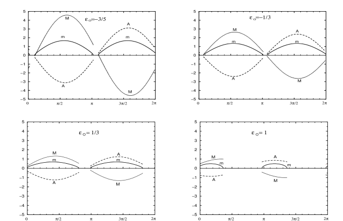
Figure 3: Soft parameters in units of $m_{3/2}$ versus $\theta$ for different values of $\epsilon_{O}$. Here $M$, $m$ and $A$ are the gaugino mass, the scalar mass and the trilinear parameter respectively.

Applying the standard (tree level) soft term formulae [40] for the above supergravity model given by (10), (11) and (12), one can compute the soft terms straightforwardly [11]

$$M = \frac{\sqrt{3}m_{3/2}}{1+\epsilon_{O}}\left(\sin\theta+\frac{1}{\sqrt{3}}\epsilon_{O}\cos\theta\right)\ ,$$

$$m^{2} = m_{3/2}^{2}-\frac{3m_{3/2}^{2}}{\left(3+\epsilon_{O}\right)^{2}}\left[\epsilon_{O}\left(6+\epsilon_{O}\right)sin^{2}\theta\right.$$

$$+ \left.\left(3+2\epsilon_{O}\right)\cos^{2}\theta-2\sqrt{3}\epsilon_{O}\sin\theta\cos\theta\right]\ ,$$

$$A = -\frac{\sqrt{3}m_{3/2}}{3+\epsilon_{O}}\left[\left(3-2\epsilon_{O}\right)\sin\theta+\sqrt{3}\epsilon_{O}\cos\theta\right]\ ,$$

where $m_{3/2}$ is the gravitino mass, and vanishing cosmological constant and phases are assumed, given the current experimental limits. Here $M$, $m$ and $A$ denote gaugino masses, scalar masses and trilinear parameters respectively. The bilinear $B$ parameter can be found in [34, 50, 27]. We are using here the parameterization introduced in [43] in order to know what fields, either $S$ or $T$, play the predominant role in the process of supersymmetry breaking $F^{S}=\sqrt{3}m_{3/2}(S+\bar{S})\sin\theta$ , $F^{T}=m_{3/2}(T+\bar{T})\cos\theta$.

As mentioned in the introduction, the structure of these soft terms is qualitatively different from that of a Calabi–Yau compactification of the (tree–level) weakly–coupled heterotic string found in [43] which can be recovered from (LABEL:softterms) by taking the limit $(T+\bar{T})\ll(S+\bar{S})$, i.e. $\epsilon_{O}\rightarrow 0$:

$$-A=M=\sqrt{3}m=\sqrt{3}m_{3/2}\sin\theta\ .$$ (25)

Clearly the M–theory result (LABEL:softterms) is more involved due to the additional dependence on $\epsilon_{O}$. Nevertheless we can simplify the analysis by taking into account the bounds (18).

We show in Fig. 3 the dependence on $\theta$ of the soft terms $M$, $m$, and $A$ in units of the gravitino mass for different values of $\epsilon_{O}$ [11, 31, 27]. Several comments are in order. First of all, some ranges of $\theta$ are forbidden by having a negative scalar mass-squared. In the weakly–coupled heterotic string case shown in Fig. 4, the forbidden region vanishes since the squared scalar masses are always positive (see (25)). About the possible range of soft terms, the smaller the value of $\epsilon_{O}$, the larger the range becomes. In the limit $\epsilon_{O}\rightarrow-1$, $0.3<|A|/m_{3/2}<4.58$, $0<m/m_{3/2}<2.26$ and $|M|\rightarrow\infty$.

In order to discuss the supersymmetric spectra further, it is worth noticing that gaugino masses are in general larger than scalar masses. This implies at low–energy ($\approx M_{W}$) the following qualitative result [11]: $M_{\tilde{g}}\approx m_{\tilde{q}}>m_{\tilde{l}}$, where $\tilde{g}$ denote the gluino, $\tilde{l}$ all the sleptons and $\tilde{q}$ first and second generation squarks. Other analyses taking into account the details of the electroweak radiative breaking can be found in [34, 35]. Only for values of $\epsilon_{O}$ approaching $-1$ the opposite situation, scalars heavier than gauginos, may occur. This is for two narrow ranges of values of $\theta$ as can be seen in Fig. 3 for $\epsilon_{O}=-3/5$. Let us remark that $M/m_{3/2}$ and $m/m_{3/2}$ are then very small and therefore $m_{3/2}$ must be large in order to fulfil e.g. the low–energy bounds on gluino masses. In this special limits $m\gg M$ is possible and then $M_{\tilde{g}}<m_{\tilde{q}}\approx m_{\tilde{l}}$ [27].

Notice that in the (tree–level) weakly–coupled heterotic string, the limit $\sin\theta\rightarrow 0$ is not well defined since all $M$, $A$, $m$ vanish in that limit. One then has to include the string one–loop corrections (or the sigma–model corrections) to the Kähler potential and gauge kinetic functions which would modify the boundary conditions (25). This is similar to what happens in orbifold compactifications where, at the end of the day, scalars are heavier than gauginos due to string loop corrections [43]. This problem is not present in the heterotic M–theory, as can be deduced from Fig. 3, except in models with $\beta_{O}=0$, i.e. $\epsilon_{O}=0$ and therefore with boundary conditions (25).

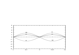
Figure 4: The same as Fig. 3 but for the weakly–coupled heterotic string limit.

3.3 Charge and colour breaking

Figure 5: Excluded regions of the parameter space.

We discussed in subsection 2.2 how effective supergravity models from heterotic M–theory can be strongly constrained by imposing the (experimental) requirement of universal soft scalar masses, in order to avoid dangerous flavour changing neutral current phenomena. We can go further and impose the (theoretical) constraint of demanding the no existence of low–energy charge and colour breaking minima deeper than the standard vacuum [36]. In this type of analysis, the form of the soft terms is crucial. In the case of the standard embedding, $0<\epsilon_{O}<1$, with soft terms given by (LABEL:softterms) the restrictions are very strong and the whole parameter space ($m_{3/2},\theta,\epsilon_{O},B$) turns out to be excluded on these grounds [37, 38]. This is shown in Fig. 5 [38] for a fixed value of $m_{3/2}$ (or, equivalently, of $m$) with $\epsilon_{O}=1$. Then we are left with two independent parameters $B$ and $\theta$. Whereas the black region is excluded because it is not possible to reproduce the experimental mass of the top, the rest is excluded by charge and colour breaking constraints. The small squares indicate regions excluded by the so–called UFB constraints and the circles indicate regions excluded by the so–called CCB constraints. Other values for $m$ and $\epsilon_{O}$ do not modify these conclusions.

Given these dramatic consequences, a way–out must be searched [51]. The first possibility is to consider the case of the non–standard embedding since although the formulae for the soft terms are the same (LABEL:softterms) the parameter space is different: $-1<\epsilon_{O}<0$. Another possible way–out is to consider the presence of five–branes in the vacuum, then the soft terms are different (see(27)) and new parameters, as e.g. the goldstino angles $\theta_{n}$ associated with $F$–terms of the five–branes, enter in the game. Possibly some regions in the parameter space will be allowed. Although now the situation is clearly more model dependent.

It is worth noticing that the situation in the perturbative heterotic string compactified on a Calabi–Yau is basically worst. There the whole parameter space ($m_{3/2},\theta,B$) is forbidden [38] and there is no the freedom of playing around with $\epsilon_{O}$ and/or $\theta_{n}$ from five–branes. Only in the limit $\sin\theta\rightarrow 0$, where one has to include loop corrections to the boundary conditions (25), small regions might be allowed. At least this is the case of orbifold compactifications with the same boundary conditions (i.e. models where all observable particles have modular weight $-1$) [38].

4 Vacua with five-branes

In the previous section, we studied the phenomenology of heterotic M–theory vacua obtained through standard and non–standard embedding. Here we want to analyze (non–perturbative) heterotic M–theory vacua due to the presence of five–branes.

4.1 Four–dimensional effective supergravity

As mentioned in the introduction, five–branes are non–perturbative objects, located at points, $x^{11}=x_{n}(n=1,...,N)$, throughout the orbifold interval. The modifications to the four–dimensional effective action determined by (10), (11) and (12), due to their presence, have recently been investigated by Lukas, Ovrut and Waldram [26, 13]. Basically, they are due to the existence of moduli, $Z_{n}$, whose ${\rm Re}(Z_{n})\equiv z_{n}=x_{n}/\pi\rho\in(0,1)$ are the five–brane positions in the normalized orbifold coordinates. Then, the effective supergravity obtained from heterotic M–theory compactified on a Calabi–Yau manifold in the presence of five–branes is now determined by

$$K = -\ln(S+\bar{S})-3\ln(T+\bar{T})+K_{5}$$

$$+ \frac{3}{T+\bar{T}}\left(1+\frac{1}{3}e_{O}\right)H_{pq}C_{O}^{p}\bar{C}_{O}^{q},$$

$$f_{O} = S+B_{O}T\ ,\quad f_{H}=S+B_{H}T\ ,$$

$$W_{O} = d_{pqr}C_{O}^{p}C_{O}^{q}C_{O}^{r}\ ,$$ (26)

with $e_{O}=b_{O}\frac{T+\bar{T}}{S+\bar{S}}$. Here $K_{5}$ is the Kähler potential for the five–brane moduli $Z_{n}$, $H_{pq}$ is some $T$–independent metric (see footnote 4) and $b_{O}=\beta_{O}+\sum_{n=1}^{N}(1-z_{n})^{2}\beta_{n}$, $B_{O}=\beta_{O}+\sum_{n=1}^{N}(1-Z_{n})^{2}\beta_{n}$, $B_{H}=\beta_{H}+\sum_{n=1}^{N}(Z_{n})^{2}\beta_{n}$, with $\beta_{O}$, $\beta_{H}$ the instanton numbers and $\beta_{n}$ the five–brane charges. The former, instead of condition (7), must fulfil now: $\beta_{O}+\sum_{n=1}^{N}\beta_{n}+\beta_{H}=0$.

4.2 Phenomenology

Assuming for simplicity that $<Z_{n}>=<z_{n}>$, i.e. $<B_{O}>=<b_{O}>$, (14) is still valid with the modification $\epsilon_{O,H}\rightarrow e_{O,H}$, where $e_{H}=b_{H}\frac{T+\bar{T}}{S+\bar{S}}$ with $b_{H}=\beta_{H}+\sum_{n=1}^{N}(z_{n})^{2}\beta_{n}$. Following the analysis of section 3 one can write $e_{O}$ as a function of $S+\bar{S}$ as in (19) and therefore the bounds for $S+\bar{S}$ in (20) and (21) are still valid if $-1<e_{O}<1$ is possible. In fact one can obtain different bounds on $e_{O}$ depending on the sign of both $b_{O}$ and $b_{H}$ [27]. For example, if $b_{H}\geq 0$ and $b_{O}\leq 0$, then $e_{H}$ is positive and $e_{O}$ negative. Since $V_{O}=V(1+e_{O})$ must be positive we need $-1<e_{O}\leq 0$. Another example is the case $b_{H}\geq 0$ and $b_{O}>0$. Now since $e_{O}$ is positive $V_{O}$ will always be positive and therefore the only bound is $e_{O}>0$. It is worth noticing that the values $0<(S+\bar{S})<2$, corresponding to $e_{O}>1$ are then possible. This was not the case in the absence of five–branes since $\epsilon_{O}>1$ was not allowed.

4.2.1 Scales

In the presence of five–branes $V=<V>$ as in section 3 is no longer true since $V_{O,H}=V(1+e_{O,H})$ with $e_{O}+e_{H}\neq 0$ in general. Therefore $\frac{V}{<V>}=\left[1+\frac{e_{O}}{2}\left(1+\frac{b_{H}}{b_{O}}\right)\right]^{-1}$ and the relevant formulae to study the relation between the different scales of the theory are (15) and (17) with the modification $\epsilon_{O}\rightarrow e_{O}$. Notice that (16) is not modified. Similarly to the case without five–branes, to obtain $V_{O}^{-1/6}\approx 3\times 10^{16}$ GeV when $T+\bar{T}$ and $S+\bar{S}$ are of order one is quite natural. To carry out the numerical analysis we can use (22) with the factor $\frac{V}{<V>}$ written above multiplying the r.h.s. and with the modifications $\epsilon_{O}\rightarrow e_{O}$, $\beta_{O}\rightarrow b_{O}$. Several examples were considered in [27]. Although the qualitative results are similar to those of Fig. 1 with $e_{O}$ instead of $\epsilon_{O}$, now the line corresponding to $V_{O}^{-1/6}$ in the r.h.s. of the figure may intersect the straight line corresponding to the GUT scale. Of course this effect, which is due essentially to the extra factor discussed above, is welcome.

Figure 6: $\log M_{11}$, $\log V_{O}^{-1/6}$ and $\log(\pi\rho)^{-1}$ versus $\log e_{O}$. The straight line corresponds to $M_{GUT}=3\times 10^{16}$ GeV.

Only in some special limits one may lower the scales. As in the case without five–branes, fine–tuning $e_{O}\rightarrow-1$ we are able to obtain $V_{O}^{-1/6}$ as low as we wish. The numerical results will be basically similar to the ones of subsection 3.1. Moreover, as discussed above, $e_{O}>1$ is possible in the presence of five–branes and therefore with $e_{O}$ sufficiently large we may get $V_{O}^{-1/6}$ very small. This is shown in Fig. 6 for the example $b_{O}=b_{H}=1/2$. For instance, with $\log e_{O}=56.1$ the experimental lower bound $(\pi\rho)^{-1}=10^{-13}$ GeV is obtained for $V_{O}^{-1/6}=8\times 10^{6}$ GeV, corresponding to $S+\bar{S}=3.1\times 10^{-56}$ and $T+\bar{T}=8$. Clearly we introduce a hierarchy problem.

Finally, the analysis of the special case $b_{O}=0$ will be similar to the one of the case $\beta_{O}=0$ without five–branes in subsection 3.1. We can use (23) with the average volume $[1+b_{H}(T+\bar{T})/8]^{-1/2}$ multiplying the r.h.s. Depending on the value of $b_{H}$ we obtain different results [27]. For example if $b_{H}>0$ the results are qualitatively similar to those of Fig. 2, the larger $T+\bar{T}$ the smaller $V_{O}^{-1/6}$ becomes. However, notice that now for large $T$ we have a factor $(T+\bar{T})^{-1}$ and then not so large values of $T+\bar{T}$ as in Fig. 2 are needed in order to lower the scales. For example, if $b_{H}=1$ then $V_{O}^{-1/6}=1$ TeV can be obtained for $T+\bar{T}=10^{14}$ with the size of the orbifold $(\pi\rho)^{-1}=5\times 10^{-12}$ GeV close to its experimental bound of $1$ millimetre. In any case, still a large hierarchy between $S+\bar{S}$ and $T+\bar{T}$ is needed.

4.2.2 Soft terms

Let us now concentrate on the computation of soft terms [13, 32, 27]. Due to the possible contribution of several $F$–terms associated with five–branes, which can have in principle off–diagonal Kähler metrics, the computation of the soft terms turns out to be extremely involved. In order to get an idea of their value and also to study the deviations with respect to the case without five–branes we can do some simplifications. One possibility is to assume that five–branes are present but only the $F$–terms associated with the dilaton and the modulus contribute to supersymmetry breaking, i.e. $F^{Z_{n}}=0$. Then, assuming as before $<Z_{n}>=<z_{n}>$, eq.(LABEL:softterms) is still valid with $e_{O}$ instead of $\epsilon_{O}$. Under these simplifying assumptions, Fig. 3 is also valid in this case since, as discussed above, the range of allowed values of $e_{O}$ includes those of $\epsilon_{O}$, i.e. $-1<e_{O}<1$. The relevant difference with respect to the case without five–branes is that now values with $e_{O}\geq 1$ are allowed. This possibility was studied in [27]. Although the soft terms are qualitatively different from those without five–branes analyzed in Fig. 3, the fact that always scalar masses are smaller than gaugino masses is still true for $e_{O}\geq 1$. As discussed below (25), we will obtain at low–energies, $M_{\tilde{g}}\approx m_{\tilde{q}}>m_{\tilde{l}}$.

Another possibility to simplify the computation of the soft terms is to assume that there is only one five–brane in the model. For example, parameterizing $F^{S}=\sqrt{3}m_{3/2}(S+\bar{S})\sin\theta\cos\theta_{1}$, $F^{T}=m_{3/2}(T+\bar{T})\cos\theta\cos\theta_{1}$, $F^{Z_{1}}=\sqrt{3}m_{3/2}\\ ({{\partial}_{1}{\partial}_{\bar{1}}K_{5}})^{-1/2}sin\theta_{1}$, where $\theta_{1}$ is the new goldstino angle associated to the $F$–term of the five–brane, one obtains [32, 27].

$$M = \frac{\sqrt{3}m_{3/2}}{\left(1+\frac{B_{O}T+\bar{B}_{O}\bar{T}}{S+\bar{S}}\right)}\left(\sin\theta\cos\theta_{1}\right.$$

$$+ \frac{1}{\sqrt{3}}B_{O}\frac{e_{O}}{b_{O}}\cos\theta\cos\theta_{1}$$

$$- \left.\frac{2T}{S+\bar{S}}(1-Z_{1})\beta_{1}({{\partial}_{1}{\partial}_{\bar{1}}K_{5}})^{-1/2}sin\theta_{1}\right)\ ,$$

$$m^{2} = m_{3/2}^{2}-\frac{3m_{3/2}^{2}}{(3+e_{O})^{2}}\left\{e_{O}(6+e_{O})\sin^{2}\theta\right.$$

$$\times \cos^{2}\theta_{1}+(3+2e_{O})\cos^{2}\theta\cos^{2}\theta_{1}$$

$$- 2\sqrt{3}e_{O}\sin\theta\cos\theta\cos^{2}\theta_{1}$$

$$+ ({{\partial}_{1}{\partial}_{\bar{1}}K_{5}})^{-1}\sin^{2}\theta_{1}\left((3+e_{O})\beta_{1}\frac{e_{O}}{2b_{O}}\right.$$

$$- \left.\left[(1-z_{1})\beta_{1}\frac{e_{O}}{b_{O}}\right]^{2}\right)+6(1-z_{1})\beta_{1}\frac{e_{O}}{b_{O}}$$

$$\times ({{\partial}_{1}{\partial}_{\bar{1}}K_{5}})^{-1/2}\sin\theta\sin\theta_{1}\cos\theta_{1}$$

$$- 2\sqrt{3}(1-z_{1})\beta_{1}\frac{e_{O}}{b_{O}}({{\partial}_{1}{\partial}_{\bar{1}}K_{5}})^{-1/2}$$

$$\times \left.\cos\theta\sin\theta_{1}\cos\theta_{1}\right\}\ ,$$

$$A = -\frac{\sqrt{3}m_{3/2}C}{3+e_{O}}\left\{(3-2e_{O})\sin\theta\cos\theta_{1}\right.$$ (27)

$$+ \sqrt{3}e_{O}\cos\theta\cos\theta_{1}-({{\partial}_{1}{\partial}_{\bar{1}}K_{5}})^{-1/2}\sin\theta_{1}$$

$$\times \left.\left[(3+e_{O}){{\partial}_{1}K_{5}}+3(1-z_{1})\beta_{1}\frac{e_{O}}{b_{O}}\right]\right\}$$

The formula for the $B$ parameter can be found in [27]. Unfortunately, the numerical analysis of this simplified case is not straightforward. All soft terms depend not only on the new goldstino angle $\theta_{1}$ in addition to $m_{3/2}$, $\theta$ and $e_{O}$, but also on other free parameters. For example, although gaugino masses can be further simplified with the assumption $<Z_{n}>=<z_{n}>$, i.e. $<B_{O}>=<\bar{B}_{O}>=<b_{O}>$ (and therefore $(B_{O}T+\bar{B}_{O}\bar{T})/(S+\bar{S})=e_{O}$), and $<T>=<\bar{T}>$ (and therefore $2T/(S+\bar{S})=e_{O}/b_{O}$), still they have an explicit dependence on $z_{1}$ and $\partial_{1}\partial_{\bar{1}}K_{5}$. Notice that, for a given model, $\beta_{O}$ and $\beta_{1}$ are known and therefore $b_{O}$ can be computed once $z_{1}$ is fixed. Something similar occurs for the $A$ parameter, where $z_{1}$, $\partial_{1}K_{5}$ and $\partial_{1}\partial_{\bar{1}}K_{5}$ appear explicitly, and for the scalar masses, where $z_{1}$ and $\partial_{1}\partial_{\bar{1}}K_{5}$ also appear. Thus in order to compute soft terms when a five–brane is present and contributing to supersymmetry breaking we have to input these values. Fortunately, $z_{1}$ is in the range $0<z_{1}<1$ and, although $K_{5}$ is not known, since it depends on $z_{1}$, we expect $\partial_{1}K_{5}$, $\partial_{1}\partial_{\bar{1}}K_{5}={\cal O}(1)$. So we can consider the following representative case: $z_{1}=1/2$ and $\partial_{1}K_{5}=\partial_{1}\partial_{\bar{1}}K_{5}=1$. Since, still we have to input the value of $b_{O}$, we choose an example with $\beta_{O}=1$ and $\beta_{1}=-2$ which implies $b_{O}=b_{H}=1/2$. Then all positive values of $e_{O}$ are allowed. We show in Fig. 7 the soft terms for the value $e_{O}=3/5$ with $\theta_{1}=\pi/3$.

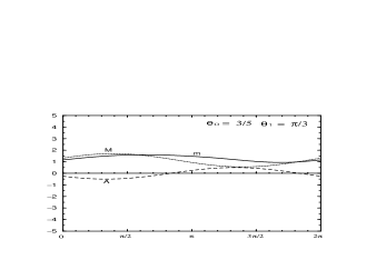
Figure 7: Soft parameters in units of $m_{3/2}$ versus $\theta$ when one five–brane is contributing to supersymmetry breaking.

Unlike Fig. 3 without five–branes, we see now a remarkable fact: scalar masses larger than gaugino masses can easily be obtained. This happens not only for narrow ranges of $\theta$. For example, for $e_{O}=1/3$ and $\theta_{1}=\pi/3$, $\theta\approx 3\pi/2$ one obtains $m/|M|\approx 10$. This result implies a relation of the type $m_{\tilde{l}}\approx m_{\tilde{q}}\approx 3.5M_{\tilde{g}}$. An exhaustive analysis of other examples can be found in [27].

Acknowledgments

This work has been supported in part by the CICYT, under contract AEN97-1678-E, and the European Union, under TMR contract ERBFMRX-CT96-0090.

References

- [1] For a review, see e.g.: J.H. Schwarz, hep-th/9807135, and references therein.
- [2] P. Hořava and E. Witten, Nucl. Phys. B460, 506 (1996); Nucl. Phys. B475, 94 (1996).
- [3] E. Witten, Nucl. Phys. B471, 135 (1996).
- [4] T. Banks and M. Dine, Nucl. Phys. B479, 173 (1996).
- [5] T. Li, J. L. Lopez and D. V. Nanopoulos, Phys. Rev. D56, 2602 (1997).
- [6] E. Dudas and C. Grojean, Nucl. Phys. B507, 553 (1997).
- [7] H. P. Nilles, M. Olechowski and M. Yamaguchi, Phys. Lett. B415, 24 (1997); Nucl. Phys. B530, 43 (1998).
- [8] K. Choi, Phys. Rev. D56, 6588 (1997).
- [9] H. P. Nilles and S. Stieberger, Nucl. Phys. B499, 3 (1997).
- [10] A. Lukas, B. A. Ovrut and D. Waldram, Nucl. Phys. B532, 43 (1998).
- [11] K. Choi, H.B. Kim and C. Muñoz, Phys. Rev. D57, 7521 (1998).
- [12] H.P. Nilles, Phys. Lett. B180, 240 (1986).
- [13] A. Lukas, B.A. Ovrut and D. Waldram, JHEP 9904, 009 (1999).
- [14] R. Donagi, A. Lukas, B.A. Ovrut and D. Waldram, JHEP 9905, 015 (1999); hep-th/9901009.
- [15] N. Wyllard, JHEP 9804, 009 (1998).
- [16] P. Hořava, Phys. Rev. D54, 7561 (1996).
- [17] Z. Lalak and S. Thomas, Nucl. Phys. B515, 55 (1998).
- [18] A. Lukas, B.A. Ovrut and D. Waldram, Phys. Rev. D57, 7529 (1998).
- [19] I. Antoniadis and M. Quiros, Phys. Lett. B416, 327 (1998); Nucl. Phys. B505, 109 (1997).
- [20] K. Choi, H.B. Kim and H. Kim, Mod. Phys. Lett. A14, 125 (1999).
- [21] B. de Carlos, J.A. Casas and C. Muñoz, Phys. Lett. B299, 234 (1993).
- [22] B. de Carlos, J. A. Casas and C. Muñoz, Nucl. Phys. B399, 623 (1993).
- [23] S. Stieberger, Nucl. Phys. B541, 109 (1999).
- [24] K. Benakli, Phys. Lett. B447, 51 (1999).
- [25] Z. Lalak, S. Pokorski and S. Thomas, hep-ph/9807503.
- [26] A. Lukas, B.A. Ovrut and D. Waldram, Phys. Rev. D59, 106005 (1999).
- [27] D.G. Cerdeño and C. Muñoz, hep-ph/9904444.
- [28] J. Lykken, Phys. Rev. D54, 3693 (1996).
- [29] I. Antoniadis, N. Arkani–Hamed, S. Dimopoulos and G. Dvali, Phys. Lett. B436, 257 (1998).
- [30] K. Benakli, hep-ph/9809582.
- [31] T. Li, hep-ph/9903371.
- [32] T. Kobayashi, J. Kubo and H. Shimabukuro, hep-ph/9904201.
- [33] T. Li, J.L. Lopez and D.V. Nanopoulos, Mod. Phys. Lett. A12, 2647 (1997).
- [34] D. Bailin, G.V. Kraniotis and A. Love, Phys. Lett. B432, 90 (1998); hep-ph/9812283.
- [35] Y. Kawamura, H.P. Nilles, M. Olechowski and M. Yamaguchi, JHEP 9806, 008 (1998).
- [36] For a review, see: C. Muñoz, hep-ph/9709329, and references therein.
- [37] S.A. Abel and C.A. Savoy, Phys. Lett. B444, 119 (1998).
- [38] J.A. Casas, A. Ibarra and C. Muñoz, hep-ph/9810266, to appear in Nucl. Phys. B.
- [39] For a review, see: C. Muñoz, hep-ph/9710388, and references therein.
- [40] For a review, see: A. Brignole, L.E. Ibanez and C. Muñoz, hep-ph/9707209, and references therein.
- [41] H.B. Kim and C. Muñoz, Z. Phys. C75, 367 (1997).
- [42] V.S. Kaplunovsky and J. Louis, Phys. Lett. B306, 269 (1993).
- [43] A. Brignole, L. E. Ibanez and C. Muñoz, Nucl. Phys. B422, 125 (1994)
- [44] J. Louis and Y. Nir, Nucl. Phys. B447, 18 (1995).
- [45] K. Choi, J.S. Lee and C. Muñoz, Phys. Rev. Lett. 80, 3686 (1998).
- [46] A. Lukas, B.A. Ovrut, K.S. Stelle and D. Waldram, hep-th/9806051.
- [47] A. Brignole, L. E. Ibanez, C. Muñoz and C. Scheich, Z. Phys. C74, 157 (1997).
- [48] L.E. Ibañez and D. Lüst, Nucl. Phys. B382, 1992 (305).
- [49] C. Burgess, L.E. Ibañez and F. Quevedo, Phys. Lett. B447, 257 (1999).
- [50] C. Kokorelis, hep-th/9810187.
- [51] J.A. Casas, A. Ibarra and C. Muñoz, in preparation.