NSF-ITP-99-040

OHSTPY-HEP-T-99-012

hep-th/9906087

Can DLCQ test the Maldacena Conjecture?

Francesco Antonuccio^a, Akikazu Hashimoto^b, Oleg Lunin^a, and Stephen Pinsky^a

^aDepartment of Physics

Ohio State University, Columbus, Ohio 43210

^bInstitute for Theoretical Physics

University of California, Santa Barbara, CA 93106

We consider the Maldacena conjecture applied to the near horizon geometry of a D1-brane in the supergravity approximation and consider the possibility of testing the conjecture against the boundary field theory calculation using DLCQ. We propose the two point function of the stress energy tensor as a convenient quantity that may be computed on both sides of the correspondence. On the supergravity side, we may invoke the methods of Gubser, Klebanov, Polyakov, and Witten. On the field theory side, we derive an explicit expression for the two point function in terms of data that may be extracted from a DLCQ calculation at a given harmonic resolution. This gives rise to a well defined numerical algorithm for computing the two point function, which we test in the context of free fermions and the ’t Hooft model. For the supersymmetric Yang-Mills theory with 16 supercharges that arises in the Maldacena conjecture, the algorithm is perfectly well defined, although the size of the numerical computation grows too fast to admit any detailed analysis at present, and our results are only preliminary. We are, however, able to present more detailed results on the supersymmetric DLCQ computation of the stress energy tensor correlators for two dimensional Yang Mills theories with (1,1) and (2,2) supersymmetries.

June 1999

1 Introduction

There has been a great deal of excitement during this past year following the realization that certain field theories admit concrete realizations as a string theory on a particular background [1]. By now many examples of this type of correspondence for field theories in various dimensions with various field contents have been reported in the literature (for a comprehensive review and list of references, see [2]). However, attempts to apply these correspondences to study the details of these theories have only met with limited success so far. The problem stems from the fact that our understanding of both sides of the correspondence is limited. On the field theory side, most of what we know comes from perturbation theory where we assume that the coupling is weak. On the string theory side, most of what we know comes from the supergravity approximation where the curvature is small. There are no known situations where both approximations are simultaneously valid. At the present time, comparisons between the dual gauge/string theories have been restricted to either qualitative issues or quantities constrained by symmetry. Any improvement in our understanding of field theories beyond perturbation theory or string theories beyond the supergravity approximation is therefore a welcome development.

In this note we raise the Supersymmetric Discrete Light Cone Quantization (SDLCQ) of field theories [3, 4, 5] to the challenge of providing quantitative data which can be compared against the supergravity approximation on the string theory side of the correspondence. We will work in two space-time dimensions where the SDLCQ approach provides a natural non-perturbative solution to the theory. In general, attempts to improve the field theory side beyond perturbation theory seem like a promising approach in two space-time dimensions where a great deal is already known about field theories beyond perturbation theory.

We will study the field theory/string theory correspondence motivated by considering the near-horizon decoupling limit of a D1-brane in type IIB string theory [6]. The gauge theory corresponding to this theory is the Yang-Mills theory in two dimensions with 16 supercharges. Its SDLCQ formulation was recently reported in [7]. This is probably the simplest known example of a field theory/string theory correspondence involving a field theory in two dimensions with a concrete Lagrangian formulation.

A convenient quantity that can be computed on both sides of the correspondence is the correlation function of gauge invariant operators [8, 9]. We will focus on two point functions of the stress-energy tensor. This turns out to be a very convenient quantity to compute for many reasons that we will explain along the way. Some aspects of this as it pertains to a consideration of black hole entropy was recently discussed in [10]. There are other physical quantities often reported in the literature. In the DLCQ literature, the spectrum of hadrons is often reported. This would be fine for theories in a confining phase. However, we expect the SYM in two dimension to flow to a non-trivial conformal fixed point in the infra-red [6, 11]. The spectrum of states will therefore form a continuum and will be cumbersome to handle. On the string theory side, entropy density [12] and the quark anti-quark potential [12, 13, 14] are frequently reported. The definition of entropy density requires that we place the field theory in a space-like box which seems incommensurate with the discretized light cone. Similarly, a static quark anti-quark configuration does not fit very well inside a discretized light-cone geometry. The correlation function of point-like operators do not suffer from these problems. We should mention that there exists interesting work on computing the QCD string tension [15, 16] directly in the field theory. These authors find that the QCD string tension vanishes in the supersymmetric theories which is consistent with the power law quark anti-quark potential found on the supergravity side.

2 Correlation functions from supergravity

Let us begin by reviewing the computation of the correlation function of stress energy tensors on the string theory side using the supergravity approximation. The computation is essentially a generalization of [8, 9]. The main conclusion on the supergravity side was reported recently in [10] but we will elaborate further on the details. The near horizon geometry of a D1-brane in string frame takes the form

$$ds^{2} = \alpha^{\prime}\left({U^{3}\over\sqrt{64\pi^{3}g_{YM}^{2}N}}dx_{\parallel}^{2}+{\sqrt{64\pi^{3}g_{YM}^{2}N}\over U^{3}}dU^{2}+\sqrt{64\pi^{3}g_{YM}^{2}N}Ud\Omega_{8-p}^{2}\right)$$

$$e^{\phi} = 2\pi g_{YM}^{2}\left({64\pi^{3}g_{YM}^{2}N\over U^{6}}\right)^{{1\over 2}}.$$ (1)

In order to compute the two point function, we need to know the action for the diagonal fluctuations around this background to the quadratic order. What we need is an analogue of [17] for this background which unfortunately is not currently available in the literature. Fortunately, some diagonal fluctuating degrees of freedom can be identified by following the early work on black hole absorption cross-sections [18, 19]. In particular, we can show that the fluctuations parameterized according to

$$ds^{2} = \left(1+f(x^{0},U)+g(x^{0},U)\right)g_{00}(dx^{0})^{2}+\left(1+5f(x^{0},U)+g(x^{0},U)\right)g_{11}(dx^{1})^{2}$$

$$+\left(1+f(x^{0},U)+g(x^{0},U)\right)g_{UU}dU^{2}+\left(1+f(x^{0},U)-{5\over 7}g(x^{0},U)\right)g_{\Omega\Omega}d\Omega_{7}^{2}$$

$$e^{\phi} = \left(1+3f(x^{0},U)-g(x^{0},U)\right)e^{\phi_{0}}$$ (2)

will satisfy the equations of motion

$$f^{\prime\prime}(U)+{7\over U}f^{\prime}(U)-{64\pi^{3}g_{YM}^{2}Nk^{2}\over U^{6}}f(U) = 0$$

$$g^{\prime\prime}(U)+{7\over U}g^{\prime}(U)-{72\over U^{2}}g(U)-{64\pi^{3}g_{YM}^{2}Nk^{2}\over U^{6}}g(U) = 0$$ (3)

by direct substitution into the equations of motion in 10 dimensions. We have assumed without loss of generality that these fluctuation vary only along the $x^{0}$ direction of the world volume coordinates like a plane wave $e^{ikx^{0}}$. The fields $f(U)$ and $g(U)$ are scalars when the D1-brane is viewed as a black hole in 9 dimensions; in fact there are the minimal and the fixed scalars in this black hole geometry. In 10 dimensions, however, we see that they are really part of the gravitational fluctuation. We expect therefore that they are associated with the stress-energy tensor in the operator field correspondence of [8, 9]. In the case of the correspondence between ${\cal N}=4$ SYM and $AdS_{5}\times S_{5}$, superconformal invariance allowed the identification of operators and fields in short multiplets [20]. For the D1-brane, we do not have superconformal invariance and this technique is not applicable. In fact, we expect all fields of the theory consistent with the symmetry of a given operator to mix. The large distance behavior should then be dominated by the contribution with the longest range. The field $f(k^{0},U)$ appears to be the one with the longest range since it is the lightest field.

The equation (3) for $f(U)$ can be solved explicitly in terms of the Bessel’s function

$$f(U)=U^{-3}K_{3/2}(\sqrt{16\pi^{3}g_{YM}^{2}N}U^{-2}k).$$ (4)

By thinking of $f(U)$ in direct analogy with the minimally coupled scalar as was done in [8, 9], we can compute the flux factor

$${\cal F}=\lim_{U_{0}\rightarrow\infty}\left.{1\over 2\kappa_{10}^{2}}\sqrt{g}g^{UU}e^{-2(\phi-\phi_{\infty})}\partial_{U}\log(f(U))\right|_{U=U_{0}}={NU_{0}^{2}k^{2}\over 2g_{YM}^{2}}-{N^{3/2}k^{3}\over 4g_{YM}}+\ldots$$ (5)

up to a numerical coefficient of order one which we have suppressed. We see that the leading non-analytic (in $k^{2}$) contribution is due to the $k^{3}$ term, whose Fourier transform scales according to

$$\langle{\cal O}(x){\cal O}(0)\rangle={N^{{3\over 2}}\over g_{YM}x^{5}}.$$ (6)

This result passes the following important consistency test. The SYM in 2 dimensions with 16 supercharges have conformal fixed points in both UV and IR with central charges of order $N^{2}$ and $N$, respectively. Therefore, we expect the two point function of stress energy tensors to scale like $N^{2}/x^{4}$ and $N/x^{4}$ in the deep UV and IR, respectively. According to the analysis of [6], we expect to deviate from these conformal behavior and cross over to a regime where supergravity calculation can be trusted. The cross over occurs at $x=1/g_{YM}\sqrt{N}$ and $x=\sqrt{N}/g_{YM}$. At these points, the $N$ scaling of (6) and the conformal result match in the sense of the correspondence principle [21].

3 Correlation functions from DLCQ

The challenge then is to attempt to reproduce the scaling relation (6), fix the numerical coefficient, and determine the detail of the cross-over behavior using SDLCQ. Ever since the original proposal [22], the question of equivalence between quantizing on a light-cone and on a space-like slice have been discussed extensively. This question is especially critical whenever a massless particle or a zero-mode in the quantization is present. It is generally believed that the massless theories can be described on the light-cone as long as we take $m\rightarrow 0$ as a limit. The issue of zero mode have been examined by many authors. Some recent accounts can be found in [23, 24, 25, 26, 27]. Generally speaking, supersymmetry seems to save SDLCQ from complicated zero-mode issues. We will not contribute much to these discussions. Instead, we will formulate the computation of the correlation function of stress energy tensor in naive DLCQ. To check that these results are sensible, we will first do the computation for the free fermions and the ’t Hooft model. Extension to SYM with 16 supercharges will be essentially straightforward, except for one caveat. In order to actually evaluate the correlation functions, we must resort to numerical analysis at the last stage of the computation. For the SYM with 16 supercharges, this problem grows too big too fast to be practical on desk top computer where the current calculations were performed. We can only provide an algorithm, which, when executed on an much more powerful computer, should reproduce (6). Nonetheless, the fact that we can define a concrete algorithm seems to be a progress in the right direction. One potential pit-fall is the fact that the computation may not show any sign of convergence. If this is the case, or if it converges to a result at odds with (6), we must go back and re-examine the issue of equivalence of forms and the issue of zero modes.

The technique of DLCQ is reviewed by many authors [5, 28] so we will be brief here. The basic idea of light-cone quantization is to parameterize the space using light cone coordinates $x^{+}$ and $x^{-}$ and to quantize the theory making $x^{+}$ play the role of time. In the discrete light cone approach, we require the momentum $p_{-}=p^{+}$ along the $x^{-}$ direction to take on discrete values in units of $p^{+}/k$ where $p^{+}$ is the conserved total momentum of the system and $k$ is an integer commonly referred to as the harmonic resolution. One can think of this discretization as a consequence of compactifying the $x^{-}$ coordinate on a circle with a period $2L={2\pi k/p^{+}}$. The advantage of discretizing the light cone is the fact that the dimension of the Hilbert space becomes finite. Therefore, the Hamiltonian is a finite dimensional matrix and its dynamics can be solved explicitly. In SDLCQ one makes the DLCQ approximation to the supercharges and these discrete representations satisfy the supersymmetry algebra. Therefore SDLCQ enjoys the improved renormalization properties of supersymmetric theories. Of course, to recover the continuum result, we must send $k$ to infinity and as luck would have it, we find that SDLCQ usually converges faster than the naive DLCQ. Of course, in the process, the size of the matrices will grow, making the computation harder and harder.

Let us now return to the problem at hand. We would like to compute a general expression of the form

$$F(x^{-},x^{+})=\langle{\cal O}(x^{-},x^{+}){\cal O}(0,0)\rangle\ .$$ (7)

In DLCQ, where we fix the total momentum in the $x^{-}$ direction, it is more natural to compute its Fourier transform

$$\tilde{F}(P_{-},x^{+})={1\over 2L}\langle{\cal O}(P_{-},x^{+}){\cal O}(-P_{-},0)\rangle\ .$$ (8)

This can naturally be expressed in a spectrally decomposed form

$$\tilde{F}(P_{-},x^{+})=\sum_{i}{1\over 2L}\langle 0|{\cal O}(P_{-})|i\rangle e^{-iP_{+}^{i}x^{+}}\langle i|{\cal O}(-P_{-},0)|0\rangle\ .$$ (9)

3.1 Free Dirac Fermions

Let us first consider evaluating this expression for the stress-energy tensor in the theory of free Dirac fermions as a simple example. The Lagrangian for this theory is

$${\cal L}=i\bar{\Psi}\partial\!\!\!/\,\Psi-m\bar{\Psi}\Psi$$ (10)

where for concreteness, we take $\gamma^{0}=\sigma^{2},\gamma^{1}=i\sigma^{1}$ and we take $\Psi=2^{-1/4}({\psi\atop\chi})$. In terms of the spinor components, the Lagrangian takes the form

$${\cal L}=i\psi^{*}\partial_{+}\psi+i\chi^{*}\partial_{-}\chi-{im\over\sqrt{2}}(\chi^{*}\psi-\psi^{*}\chi)\ .$$ (11)

Since we treat $x^{+}$ as time and since $\chi$ does not have any derivatives with respect to $x^{+}$ in the Lagrangian, it can be eliminated from the equation of motion, leaving a Lagrangian which depends only on $\psi$:

$${\cal L}=i\psi^{*}\partial_{+}\psi+i{m^{2}\over 2}\psi^{*}{1\over\partial_{-}}\psi\ .$$ (12)

We can therefore express the canonical momentum and energy as

$$P_{-} = \int dx^{-}\,i\psi^{*}\partial_{-}\psi$$

$$P_{+} = \int dx^{-}\,-{im^{2}\over 2}\psi^{*}{1\over\partial_{-}}\psi\ .$$ (13)

In DLCQ, we compactify $x^{-}$ to have period $2L$. We can then expand $\psi$ and $\psi^{*}$ in modes

$$\psi={1\over\sqrt{2L}}\left(b(n)e^{-{in\pi\over L}x^{-}}+d(-n)e^{{in\pi\over L}x^{-}}\right)$$

$$\psi^{*}={1\over\sqrt{2L}}\left(b(-n)e^{{in\pi\over L}x^{-}}+d(n)e^{-{in\pi\over L}x^{-}}\right)\ .$$ (14)

Operators $b(n)$ and $d(n)$ with positive and negative $n$ are interpreted as a destruction and creation operators, respectively. In a theory with only fermions, it is customary to take anti-periodic boundary condition in order to avoid zero-mode issues. Therefore, $n$ will take on half-integer values. They satisfy the anticommutation relation

$$\{b(n),b(-m)\}=\{d(n),d(-m)\}=\delta_{n,m}\ .$$ (15)

Now we are ready to evaluate (9) in DLCQ. As a simple and convenient choice, we take

$${\cal O}(-k)={1\over 2}\int dx^{-}\,\left(i\psi^{*}\partial_{-}\psi-i(\partial_{-}\psi^{*})\psi\right)e^{-{ik\pi\over L}x^{-}}.$$ (16)

which is the Fourier transform of the local expression for $P_{-}$ with the total derivative contribution adjusted to make this operator Hermitian. Therefore, this should be thought of as the $T^{++}$ component of the stress energy tensor. For reasons that will become clear as we go on, this turns out to be one of the simplest things to compute. When acted on the vacuum, this operator creates a state

$$T^{++}(-k)|0\rangle={\pi\over L}\left({k\over 2}-n\right)b(-k+n)d(-n)|0\rangle\ .$$ (17)

Since the fermions in this theory are free, the plane wave states

$$|n\rangle=b(-k+n)d(-n)|0\rangle$$ (18)

constitute an eigenstate. The spectrum can easily be determined by commuting these operators:

$$M^{2}_{n}|n\rangle=2P_{-}P_{+}|n\rangle={m^{2}}\left({k\over n}+{k\over k-n}\right)|n\rangle$$ (19)

which is simply the discretized version of the spectrum of a two body continuum. All that we have to do now is calculate eigenstates of the actual theory we are interested in and to assemble these pieces into (9), but we can do a little more to make the result more presentable. The point is that since (9) is expressed in mixed momentum/position space notation in Minkowski space, the answer is inherently a complex quantity that is cumbersome to display. For the computation of two point function, however, we can go to position space by Fourier transforming with respect to the $L$ variable. After Fourier transforming, it is straight forward to Euclideanize and display the two point function as a purely real function without loosing any information. To see how this works, let us write (9) in the form

$$\tilde{F}(P_{-},x^{+})=\left|{L\over\pi}\langle 0|T^{++}(k)|n\rangle\right|^{2}{1\over 2L}{\pi^{2}\over L^{2}}e^{-iM^{2}_{n}\over 2({k\pi\over L})x^{+}}\ .$$ (20)

The quantity inside the absolute value sign is designed to be independent of $L$. Now, to recover the position space form of the correlation function, we inverse Fourier transform with respect to $P_{-}=k\pi/L$.

$$F(x^{-},x^{+})=\left|{L\over\pi}\langle 0|T^{++}(k)|n\rangle\right|^{2}\int{d\left({k\pi\over L}\right)\over 2\pi}{1\over 2L}{\pi^{2}\over L^{2}}e^{-i{M^{2}_{n}\over 2({k\pi\over L})}x^{+}-i{k\pi\over L}x^{-}}.$$ (21)

The integral over $L$ can be done explicitly and gives

$$F(x^{-},x^{+})=\left|{L\over\pi}\langle 0|T^{++}(k)|n\rangle\right|^{2}\left({x^{+}\over x^{-}}\right)^{2}{M_{n}^{4}\over 8\pi^{2}k^{3}}K_{4}\left(M_{n}\sqrt{2x^{+}x^{-}}\right)$$ (22)

where $K_{4}(x)$ is the 4-th modified Bessel’s function. We can now continue to Euclidean space by taking $r^{2}=2x^{+}x^{-}$ to be real and considering the quantity

$$\left({x^{-}\over x^{+}}\right)^{2}F(x^{-},x^{+})=\left|{L\over\pi}\langle 0|T^{++}(k)|n\rangle\right|^{2}{M_{n}^{4}\over 8\pi^{2}k^{3}}K_{4}(M_{n}r)\ .$$ (23)

This is a fundamental result which we will refer to a number of times in this paper. It has explicit dependence on the harmonic resolution parameter $k$, but all dependence on unphysical quantities such as the size of the circle in the $x^{-}$ direction and the momentum along that direction have been canceled. For the free fermion model, (23) evaluates to

$$\left({x^{-}\over x^{+}}\right)^{2}F(x^{-},x^{+})={N\over k}\sum_{n}{M_{n}^{4}\over 32\pi^{2}}{(k-2n)^{2}\over k^{2}}K_{4}(M_{n}r)$$ (24)

with $M_{n}^{2}$ given by (19). The large $k$ limit can be gotten by replacing $n\rightarrow kx$ and ${1\over k}\sum_{n}\rightarrow\int_{0}^{1}dx$. We recover the identical result using Feynman rules. For $r\ll m^{-1}$, this behaves like

$$\left({x^{-}\over x^{+}}\right)^{2}F(x^{-},x^{+})={N\over k}\sum_{n}{3(k-2n)^{2}\over 2\pi^{2}k^{2}r^{4}}\rightarrow{N\over 2\pi^{2}r^{4}}\ .$$ (25)

3.2 ’t Hooft Model

Let us now turn to a slightly more interesting problem of computing the correlation function of $T^{++}$ in ’t Hooft’s model of two dimensional QCD [29] in the large $N$ limit. This theory has two characteristic scales, one determined by the mass of the quarks and the other by the strength of the gauge coupling $g_{YM}^{2}N$. To a large extent, this is a solvable model. The spectrum and the wave function of the hadrons are encoded in a one parameter integral equation that can be handled in many ways. A thorough analysis of this model including the discussion of asymptotic behavior of certain correlation functions can be found in [30]. This is clearly a very mature subject.

Applying DLCQ to the ’t Hooft model is tantamount to placing ’t Hooft’s integral equation for the meson spectrum on a lattice. The lattice is in the light-cone momentum space, which is precisely what is expected when the light-cone is compactified on a circle. The DLCQ of the ’t Hooft model was analyzed in detail by [31, 32].

Our goal here is to show that the computation of (9) is straight forward and that it generates sensible answers. In fact, nothing could be simpler. The ’t Hooft model is nothing more than a gauged version of the free fermion model. The Lagrangian for this theory is simply

$${\cal L}=-{1\over 4g_{YM}^{2}}F^{2}+i\bar{\Psi}D\!\!\!\!/\,\Psi-m\bar{\Psi}\Psi\ .$$ (26)

We choose the light cone gauge $A^{+}=0$ which is customary. One then finds that the $A^{-}$ component of the gauge field is non-dynamical and can be eliminated using the equation of motion, just like the $\chi$ component of the spinor in the free fermion model. Expressing everything in terms of the only dynamical field in this theory which is $\psi$, one finds the canonical energy and momentum operators to take the form

$$P_{-} = \int dx^{-}\,i\psi^{*}\partial_{-}\psi$$

$$P_{+} = \int dx^{-}\,\left(-{im^{2}\over 2}\psi^{*}{1\over\partial_{-}}\psi-{g_{YM}^{2}\over 2}J_{-}{1\over\partial_{-}^{2}}J_{-}\right)$$ (27)

where $J_{-}=\psi\psi^{*}$. All that changed in comparison to the free fermion model is the addition of a current exchange term in the light-cone Hamiltonian. Therefore, all we have to do here is to perform the identical computation specified by (23), but using the modified Hamiltonian, and letting $M^{2}_{n}$ and $|n\rangle$ be the spectrum and the wavefunction of the $n$-th meson state in the spectrum. Since in DLCQ we are always working with a finite dimensional representation of the Hamiltonian dynamics, a small change in the form of the Hamiltonian matrix causes no particular difficulty. Let us discuss the result of such a computation. We will consider the case when $g_{YM}^{2}N\gg m^{2}$ so that the effect of the gauge interaction is strong. The spectrum can be computed reliably for large $k$ and is in agreement with the results reported in [29] (see figure 1.a). Since the state (17) created by operator (16) is odd under parity $n\leftrightarrow k-n$, only parity odd states contribute in the spectral decomposition. For $r\ll 1/g_{YM}\sqrt{N}$, we expect the correlation function to behave just like the free fermion. The lightest meson in the parity odd sector has a mass of order $g_{YM}\sqrt{N}$. Due to the presence of this mass-gap, for $r\gg 1/g_{YM}\sqrt{N}$, we expect to see an exponential damping of the correlation function.

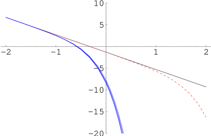
(a)	(b)

Figure 1: (a) Mass spectrum in units of $g_{YM}^{2}N/\pi$ as a function of $1/k$ and (b) Log-Log plot of the Correlation function ${1\over N}\langle T^{++}(r)T^{++}(0)\rangle$ as a function of $r$ for ’t Hooft model computed using DLCQ with $k=5$, $k=10$, $k=50$, and $k=100$ in the units where $g_{YM}\sqrt{N/\pi}=10^{1}$ and $m=10^{-1}$. The dotted line is for the free fermions with the same mass.

This is precisely the behavior we seem to be finding. In figure 1.b, we illustrate the result of computing (23) by first constructing the mass matrix $M^{2}$ symbolically, then evaluating the spectrum and the eigenfunctions numerically and assembling the pieces. We have chosen to set $g_{YM}\sqrt{N/\pi}=10^{1}$ and $m=10^{-1}$. We have tried harmonic resolutions $k=5$, $k=10$, $k=50$, and $k=100$. Remarkably, the computation at a low harmonic resolution $k$ seems not to be so far off from the result found using larger values of $k$. The correlation function appears to have more or less converged by the time we reach $k=100$. We have also included a plot for $g_{YM}^{2}N=0$ with the same mass for comparison.

One of the reasons why the convergence is relatively rapid is the fact that the matrix element $\langle 0|T^{++}(k)|n\rangle$ in (23) is not sensitive to the structure of the ’t Hooft wave function at the boundaries. To see this more clearly, recall that in the continuum limit, we expect the eigenfunctions $|n\rangle$ to behave as $x^{\beta}$ near $x=0$ where $\beta$ is determined by

$$0={m^{2}\over g_{YM}^{2}N/\pi}+\pi\beta\cot(\pi\beta)-1\approx{m^{2}\over g_{YM}^{2}N/\pi}-{\pi^{2}\beta^{2}\over 3}$$ (28)

for small $m^{2}/g_{YM}^{2}N$ [29]. When we compute matrix elements in DLCQ approximation, we are effectively exchanging integral expression like

$$\int_{0}^{1}dx\,ax^{a-1}=1$$ (29)

by a discretized sum

$$\sum_{k=1}^{n}{ak^{a-1}\over n^{a}}\sim 1+{a\zeta(1-a)\over n^{a}}+{\cal O}(n^{-1})$$ (30)

whose leading correction for $a>1$ is dominated by the terms of order $1/n$. For $a$ less than one, however, the leading correction is controlled by terms of order $({1\over n})^{a}$. In computing the form factor for $T^{++}(k)$, we were fortunate to have only encountered an integral whose end point behavior went as $x^{1+\beta}$. Had we instead chosen to compute two point function of a scalar operators like $\bar{\psi}\psi$ or $\bar{\psi}\gamma^{5}\psi$, we would have considered states

$$\int dx^{-}\,\bar{\psi}\psi(x^{-})e^{-{ik\pi\over L}x^{-}}|0\rangle = \sum_{n}{mL\over 2\pi}\left({1\over n}-{1\over k-n}\right)b(-n)d(-k+n)|0\rangle$$

$$\int dx^{-}\,\bar{\psi}\gamma^{5}\psi(x^{-})e^{-{ik\pi\over L}x^{-}}|0\rangle = \sum_{n}{mL\over 2\pi}\left({1\over n}+{1\over k-n}\right)b(-n)d(-k+n)|0\rangle$$ (31)

which gives rise to a pole near $x=0$ and $x=1$ in the continuum limit. Therefore, the matrix element in the continuum limit behaves near $x=0$ as $x^{\beta}$. To control the error in this case, we must take

$${\beta\over n^{\beta}}\ll\epsilon$$ (32)

or equivalently

$$n\gg\left(\beta\over\epsilon\right)^{1/\beta}$$ (33)

which grows exponentially with respect to $\beta^{-1}$. We would have had to work much harder if we had sent $m/g_{YM}\sqrt{N}$ to zero. Luckily, this is not the case for with the $T^{++}$ operator.

3.3 Supersymmetric Yang-Mills theory with 16 supercharges

Finally, let us turn to the problem of computing the two point function of the $T^{++}$ operator for the SYM with 16 supercharges. Just as in the ’t Hooft model, adopting light-cone coordinates and choosing the light-cone gauge will eliminate the gauge boson and half of the fermion degrees of freedom. The most significant change comes from the fact that the fields in this theory are in the adjoint rather than the fundamental representations and the theory is supersymmetric. This does not cause any fundamental problem in the DLCQ formulation of these theories. Indeed, the SDLCQ formulation of this [7] as well as many other related models with adjoint fields have been studied in the literature. The main difficulty comes from the fact that in supersymmetric theories low mass states such as ${\rm tr}[b(-n_{1})b(-n_{2})b(-k+n_{1}+n_{2})]|0\rangle$ with an arbitrary number of excited quanta, or “bits,” appear in the spectrum. This means that for a given harmonic resolution $k$, the dimension of the Hilbert space grows like $\exp(\sqrt{k})$, which is roughly the number of ways to partition $k$ into sums of integers.

The fact that the size of the problem grows very fast is somewhat discouraging from a numerical perspective. Nevertheless, it is interesting to note that DLCQ provides a well defined algorithm for computing a physical quantity like the two point function of $T^{++}$ that can be compared with the prediction from supergravity. In the following, we will show that this can be computed for the SYM theory by a straight forward application of (23), just as we saw in the case of the ’t Hooft model.

The authors of [7] have shown that the momentum operator $P^{+}$ is given by

$$P^{+}=\int dx^{-}{\rm tr}\left[(\partial_{-}X_{I})^{2}+iu_{\alpha}\partial_{-}u_{\alpha}\right].$$ (34)

The local Hermitian form of this operator is given by

$$T^{++}(x)={\rm tr}\left[(\partial_{-}X^{I})^{2}+{1\over 2}\left(iu^{\alpha}\partial_{-}u^{\alpha}-i(\partial_{-}u^{\alpha})u^{\alpha}\right)\right],\qquad I=1\ldots 8,\quad\alpha=1\ldots 8$$ (35)

where $X$ and $u$ are the physical adjoint scalars and fermions respectively, following the notation of [7]. When discretized, these operators have the mode expansion

$$X_{i,j}^{I} = {1\over\sqrt{4\pi}}\sum_{n=1}^{\infty}{1\over\sqrt{n}}\left[A^{I}_{ij}(n)e^{-i\pi nx^{-}/L}+A^{I}_{ji}(-n)e^{i\pi nx^{-}/L}\right]$$

$$u_{i,j}^{\alpha} = {1\over\sqrt{4L}}\sum_{n=1}^{\infty}\left[B^{\alpha}_{ij}(n)e^{-i\pi nx^{-}/L}+B^{\alpha}_{ji}(-n)e^{i\pi nx^{-}/L}\right].$$ (36)

In terms of these mode operators, we find

$$T^{++}(-k)|0\rangle={\pi\over 2L}\sum_{n=1}^{k-1}\left[-\sqrt{n(k-n)}A_{ij}(-k+n)A_{ji}(-n)+\left({k\over 2}-n\right)B_{ij}(-k+n)B_{ji}(-n)\right]|0\rangle.$$ (37)

Therefore, $(L/\pi)\langle 0|T^{++}(-k)|n\rangle$ is independent of $L$ and can be substituted directly into (23) to give an explicit expression for the two point function.

We see immediately that (37) has the correct small $r$ behavior, for in that limit, (37) asymptotes to (assuming $n_{b}=n_{f}$)

$$\left({x^{-}\over x^{+}}\right)^{2}F(x^{-},x^{+})={N^{2}\over k}\sum_{n}\left({3(k-2n)^{2}n_{f}\over 4\pi^{2}k^{2}r^{4}}+{3n(k-n)n_{b}\over\pi^{2}k^{2}r^{4}}\right)={N^{2}(2n_{b}+n_{f})\over 4\pi^{2}r^{4}}\left(1-{1\over k}\right)$$ (38)

which is what we expect for the theory of $n_{b}$ free bosons and $n_{f}$ free fermions in the large $k$ limit.

Computing this quantity beyond the small $r$ asymptotics, however, represents a formidable technical challenge. The authors of [7] were able to construct the mass matrix explicitly and compute the spectrum for $k=2$, $k=3$, and $k=4$. Even for these modest values of the harmonic resolution, the dimension of the Hilbert space was as big as 256, 1632, and 29056 respectively (the symmetries of the theory can be used to reduce the size of the calculation somewhat). In figure 2, we display results that parallel those obtained for the ’t Hooft model earlier (figure 1) with the currently available values of $k$, except for the fact that we display the correlation function multiplied by a factor of $4\pi^{2}r^{4}/N^{2}(2n_{b}+n_{f})$, so that it now asymptotes to 1 (or 0 in the logarithmic scale) in the $k\rightarrow\infty$ limit. In this way any deviation from the asymptotic behavior $1/r^{4}$ is made more transparent. Note that with the values of the harmonic resolution $k$ obtained at present, the spectrum in figure 2.a is far from resembling a dense continuum near $M=0$. Clearly, we must probe much higher values of $k$ before we can sensibly compare our field theory results with the prediction from supergravity.

(a)	(b)

Figure 2: (a) The spectrum as a function of $1/k$ and (b) the Log-Log plot of the correlation function $\langle T^{++}(x)T^{++}(0)\rangle\left({x^{-}\over x^{+}}\right)^{2}{4\pi^{2}r^{4}\over N^{2}(2n_{b}+n_{f})}$ v.s. $r$ in the units where $g_{YM}^{2}N/\pi=1$ for $k=3$ and $k=4$.

3.4 Supersymmetric Yang-Mills theory with less than 16 supercharges

The computation of the correlator for the stress energy tensor in the (8,8) model is limited by our inability to carry out the computation for large enough harmonic resolution. It is the (8,8) model which we are ultimately interested in solving in order to compare against the prediction of Maldacena’s conjecture in the supergravity limit. Nevertheless, the computation of the correlation function can just as well be applied to models with less supersymmetry. We will conclude by reporting the results of such a computation.

First, let us consider the theory with supercharges (1,1). This theory is argued not to exhibit dynamical supersymmetry breaking in [33, 34]. We can also provide a physicist’s proof that supersymmetry is not spontaneously broken for this theory by adopting the argument of Witten for the 2+1 dimensional SYM with Chern-Simons interaction [35]. In [35], the index of 2+1 dimensional SYM with gauge group $SU(N)$ and 2 supercharges on $R\times T^{2}$ was computed and was found to be non-vanishing for Chern-Simons coupling $k_{3}>N/2$. If the period $L$ of one of the circles in $T^{2}$ is sufficiently small, this theory is approximately the 2-dimensional SYM with (1,1) supersymmetry with gauge coupling $g_{2}^{2}=g_{3}^{2}/L$ and BF coupling $k_{2}=k_{3}L$ [36]. Imagine approaching this theory by taking $L\rightarrow 0$ keeping $g_{2}$ and $k_{3}$ fixed. In this limit, $k_{2}\rightarrow 0$ in the units of $g_{2}$ so the limiting theory is that of pure SYM with (1,1) supersymmetry and a vanishing BF coupling. Choosing different values of $k_{3}$ corresponds to a different choice in the path of approach to this limit. If we chose $k_{3}>N/2$, we are guaranteed to have a non-zero index for finite $L$. This means that there will be a state with zero mass in the $L\rightarrow 0$ limit also, indicating that supersymmetry is not spontaneously broken in this limit. On the other hand, the index is not a well defined quantity in the $L\rightarrow 0$ limit, as a different choice of $k_{3}$ will lead to a different value of the index in the $L\rightarrow 0$ limit. In fact, the index can be made arbitrarily large by taking $k_{3}$ to be also arbitrarily large. This suggests that there are infinitely many states forming a continuum near $m=0$. The index is therefore an ill defined quantity, akin to counting the number of exactly zero energy states on a periodic box as one takes the volume to infinity.

This theory is also believed not to be confining [15, 16] and is therefore expected to exhibit non-trivial infra-red dynamics.

The SDLCQ of the 1+1 dimensional model with (1,1) supersymmetry was solved in [37, 38], and we apply these results directly in order to compute (23). For simplicity, we work to leading order in the large $N$ expansion. The spectrum of this theory for various values of $k$, and the subsequent computation of (23) is illustrated in figure 3.a.

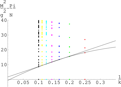
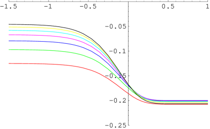
(a)	(b)

Figure 3: (a) The spectrum as a function of $1/k$ and (b) the Log-Log plot of the correlation function $\langle T^{++}(x)T^{++}(0)\rangle\left({x^{-}\over x^{+}}\right)^{2}{4\pi^{2}r^{4}\over N^{2}(2n_{b}+n_{f})}$ v.s. $r$ in the units where $g_{YM}^{2}N/\pi=1$ for $k=4\ldots 10$.

The spectrum of this theory at finite $k$, illustrated in figure 3.a, consists of $2k-2$ exactly massless states, accompanied by large numbers of massive states separated by a gap. The gap appears to be closing in the limit of large $k$ however. We have tried extrapolating the mass of the lightest massive state as a function of $1/k$ by performing a least square fit to a line and a parabola, giving the extrapolated value of $M^{2}\pi/g_{YM}^{2}N=1.7$ and $M^{2}\pi/g_{YM}^{2}N=-0.6$, suggesting indeed that at large $k$, the gap is closed. This is consistent with the expectation that the spectrum is that of a continuum starting at $M=0$ discussed earlier, although one must be careful when the order of large $N$ and large $k$ limits are exchanged. At finite $N$, we expect the degeneracy of $2k-2$ exactly massless states to be broken, giving rise to precisely a continuum of states starting at $M=0$ as expected.

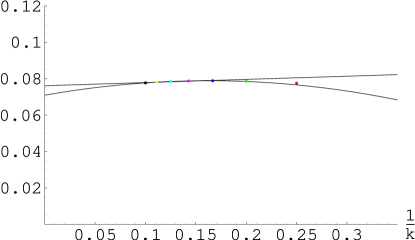
Figure 4: ${1\over k^{3}}\sum_{n}|{L\over\pi}\langle 0|T^{++}(k)|n\rangle|^{2}$ v.s. $k$ from states with $M|n\rangle=0$. This quantity determines the coefficient of the $1/r^{4}$ asymptotic tail of the correlation function in the large $r$ limit for the (1,1) model.

In the computation of the correlation function illustrated in figure 3.b, we find a curious feature that it asymptotes to the inverse power law $c/r^{4}$ for large $r$. This behavior comes about due to the coupling $\langle 0|T^{++}|n\rangle$ with exactly massless states $|n\rangle$. The contribution to (23) from strictly massless states are given by

$$\left(x^{-}\over x^{+}\right)^{2}F(x^{-},x^{+})=\left.\left|{L\over\pi}\langle 0|T^{++}(k)|n\rangle\right|^{2}{M_{n}^{4}\over 8\pi^{2}k^{3}}K_{4}(M_{n}r)\right|_{M_{n}=0}=\left|{L\over\pi}\langle 0|T^{++}(k)|n\rangle\right|^{2}_{M_{n}=0}{6\over k^{3}\pi^{2}r^{4}}.$$ (39)

We have computed this quantity as a function of $1/k$ and extrapolated to $1/k\rightarrow 0$ by fitting a line and a parabola to the computed values for finite $1/k$. The result of this extrapolation is illustrated in figure 4. The data currently available suggests that the non-zero contribution from these massless states persists in the large $k$ limit.

Let us now turn to the model with (2,2) supersymmetry. The SDLCQ version of this model was solved in [39]. The result of this computation can be applied to (23). The result is summarized in figure 5. This model appears to exhibit the onset of a gapless continuum of states more rapidly than the (1,1) model as the harmonic resolution $k$ is increased. Just as we found in the (1,1) model, this theory contains exactly massless states in the spectrum. These massless states appear to couple to $T^{++}|0\rangle$ only for $k$ even, and the overlap appears to be decreasing as $k$ is increased. We believe that this model is likely to exhibit a power law behavior $c/r^{\gamma}$ for $\gamma>4$ for the $T^{++}$ correlator for $r\gg g_{YM}\sqrt{N}$ in the large $N$ limit. Unfortunately, the existing numerical data do not permit the reliable computation of the exponent $\gamma$.

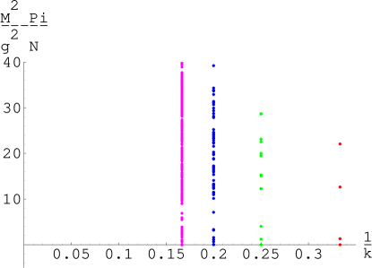
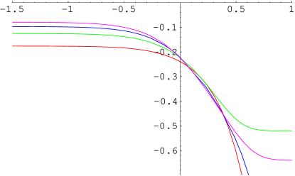
(a)	(b)

Figure 5: (a) The spectrum as a function of $1/k$ and (b) the Log-Log plot of the correlation function $\langle T^{++}(x)T^{++}(0)\rangle\left({x^{-}\over x^{+}}\right)^{2}{4\pi^{2}r^{4}\over N^{2}(2n_{b}+n_{f})}$ v.s. $r$ in the units where $g_{YM}^{2}N/\pi=1$ for $k=3\ldots 6$.

4 Conclusion

In this article, we have provided a prescription for computing the correlation function of the stress energy tensor $T^{++}$ in the SDLCQ formalism, which may be readily compared with predictions provided by a supergravity analysis following the conjecture of Maldacena. Such a comparison requires non-perturbative methods on the field theory side, and the SDLCQ approach appears at first sight to be particularly well suited to this task. Unfortunately, at the present time, high enough resolution calculation have not been made to evaluate expression (23) accurately enough in the case of SYM with 16 supercharges to reproduce (6). Significant progress is expected however when these calculation are moved from desk top computers to a supercomputer. Ultimately the main obstacle will be that the number of allowed states in the SDLCQ wavefunctions grows exponentially with the resolution. Nevertheless, a concrete well defined algorithm is a great starting point for further investigations, and additional insight may be gained by studying models with less supersymmetry, as we have done here.

Thus, the answer to the question posed in the title is a qualified “yes.” Equation (23) may be compared against (6) using SDLCQ, and unless other computational approaches such as the lattice technique catches up, the SDLCQ approach remains the most viable option.

References

- [1] J. Maldacena, “The Large N limit of superconformal field theories and supergravity,” Adv. Theor. Math. Phys. 2 (1998) 231, hep-th/9711200.
- [2] O. Aharony, S. S. Gubser, J. Maldacena, H. Ooguri, and Y. Oz, “Large N field theories, string theory and gravity,” hep-th/9905111.
- [3] T. Maskawa and K. Yamawaki, “The problem of mode in the null plane field theory and Dirac’s method of quantization,” Prog. Theor. Phys. 56 (1976) 270.
- [4] H. C. Pauli and S. J. Brodsky, “Discretized light cone quantization: solution to a field theory in one space one time dimensions,” Phys. Rev. D32 (1985) 2001.
- [5] S. J. Brodsky, H.-C. Pauli, and S. S. Pinsky, “Quantum chromodynamics and other field theories on the light cone,” Phys. Rept. 301 (1998) 299, hep-ph/9705477.
- [6] N. Itzhaki, J. M. Maldacena, J. Sonnenschein, and S. Yankielowicz, “Supergravity and the large N limit of theories with sixteen supercharges,” Phys. Rev. D58 (1998) 046004, hep-th/9802042.
- [7] F. Antonuccio, O. Lunin, S. Pinsky, H. C. Pauli, and S. Tsujimaru, “The DLCQ spectrum of N=(8,8) superYang-Mills,” Phys. Rev. D58 (1998) 105024, hep-th/9806133.
- [8] S. S. Gubser, I. R. Klebanov, and A. M. Polyakov, “Gauge theory correlators from noncritical string theory,” Phys. Lett. B428 (1998) 105, hep-th/9802109.
- [9] E. Witten, “Anti-de Sitter space and holography,” Adv. Theor. Math. Phys. 2 (1998) 253, hep-th/9802150.
- [10] A. Hashimoto and N. Itzhaki, “A Comment on the Zamolodchikov c function and the black string entropy,” hep-th/9903067.
- [11] R. Dijkgraaf, E. Verlinde, and H. Verlinde, “Matrix string theory,” Nucl. Phys. B500 (1997) 43, hep-th/9703030.
- [12] A. Brandhuber, N. Itzhaki, J. Sonnenschein, and S. Yankielowicz, “Wilson loops, confinement, and phase transitions in large N gauge theories from supergravity,” JHEP 06 (1998) 001, hep-th/9803263.
- [13] S.-J. Rey and J. Yee, “Macroscopic strings as heavy quarks in large N gauge theory and anti-de Sitter supergravity,” hep-th/9803001.
- [14] J. Maldacena, “Wilson loops in large N field theories,” Phys. Rev. Lett. 80 (1998) 4859, hep-th/9803002.
- [15] A. Armoni, Y. Frishman, and J. Sonnenschein, “Screening in supersymmetric gauge theories in two- dimensions,” Phys. Lett. B449 (1999) 76, hep-th/9807022.
- [16] A. Armoni, Y. Frishman, and J. Sonnenschein, “The String tension in two-dimensional gauge theories,” hep-th/9903153.
- [17] H. J. Kim, L. J. Romans, and P. van Nieuwenhuizen, “Mass spectrum of chiral ten-dimensional supergravity on ,” Phys. Rev. D32 (1985) 389–399.
- [18] M. Krasnitz and I. R. Klebanov, “Testing effective string models of black holes with fixed scalars,” Phys. Rev. D56 (1997) 2173–2179, hep-th/9703216.
- [19] S. S. Gubser, A. Hashimoto, I. R. Klebanov, and M. Krasnitz, “Scalar absorption and the breaking of the world volume conformal invariance,” Nucl. Phys. B526 (1998) 393, hep-th/9803023.
- [20] S. Ferrara, C. Fronsdal, and A. Zaffaroni, “On N=8 supergravity on AdS(5) and N=4 superconformal Yang- Mills theory,” Nucl. Phys. B532 (1998) 153, hep-th/9802203.
- [21] G. T. Horowitz and J. Polchinski, “A Correspondence principle for black holes and strings,” Phys. Rev. D55 (1997) 6189–6197, hep-th/9612146.
- [22] P. A. M. Dirac, “Forms of relativistic dynamics,” Rev. Mod. Phys. 21 (1949) 392.
- [23] S. Hellerman and J. Polchinski, “Compactification in the lightlike limit,” Phys. Rev. D59 (1999) 125002, hep-th/9711037.
- [24] M. Burkardt, F. Antonuccio, and S. Tsujimaru, “Decoupling of zero modes and covariance in the light front formulation of supersymmetric theories,” Phys. Rev. D58 (1998) 125005, hep-th/9807035.
- [25] F. Antonuccio, S. Pinsky, and S. Tsujimaru, “A Comment on the light cone vacuum in (1+1)-dimensional superYang-Mills theory,” hep-th/9810158.
- [26] F. Antonuccio, O. Lunin, S. Pinsky, and S. Tsujimaru, “The Light cone vacuum in (1+1)-dimensional superYang-Mills theory,” hep-th/9811254.
- [27] K. Yamawaki, “Zero mode problem on the light front,” hep-th/9802037.
- [28] K. Demeterfi and I. R. Klebanov, “Matrix models and string theory,”. Lectures given at Spring School on String Theory, Gauge Theory and Quantum Gravity, Trieste, Italy, 19-27 Apr 1993.
- [29] G. ’t Hooft, “A Two-Dimensional Model for Mesons,” Nucl. Phys. B75 (1974) 461.
- [30] C. G. Callan, N. Coote, and D. J. Gross, “Two-Dimensional Yang-Mills Theory: A Model of Quark Confinement,” Phys. Rev. D13 (1976) 1649.
- [31] K. Hornbostel, S. J. Brodsky, and H. C. Pauli, “Light Cone Quantized QCD in (1+1)-Dimensions,” Phys. Rev. D41 (1990) 3814.
- [32] K. Hornbostel, “The Application of Light Cone Quantization to Quantum Chromodynamics in (1+1)-Dimensions,”. PhD Thesis, SLAC-0333.
- [33] M. Li, “Large N solution of the 2-d supersymmetric Yang-Mills theory,” Nucl. Phys. B446 (1995) 16–34, hep-th/9503033.
- [34] H. Oda, N. Sakai, and T. Sakai, “Vacuum structures of supersymmetric Yang-Mills theories in (1+1)-dimensions,” Phys. Rev. D55 (1997) 1079–1090, hep-th/9606157.
- [35] E. Witten, “Supersymmetric index of three-dimensional gauge theory,” hep-th/9903005.
- [36] D. Birmingham, M. Blau, M. Rakowski, and G. Thompson, “Topological field theory,” Phys. Rept. 209 (1991) 129–340.
- [37] Y. Matsumura, N. Sakai, and T. Sakai, “Mass spectra of supersymmetric Yang-Mills theories in (1+1)-dimensions,” Phys. Rev. D52 (1995) 2446–2461, hep-th/9504150.
- [38] F. Antonuccio, O. Lunin, and S. Pinsky, “Nonperturbative spectrum of two-dimensional (1,1) superYang-Mills at finite and large N,” Phys. Rev. D58 (1998) 085009, hep-th/9803170.
- [39] F. Antonuccio, H. C. Pauli, S. Pinsky, and S. Tsujimaru, “DLCQ bound states of N=(2,2) super Yang-Mills at finite and large N,” Phys. Rev. D58 (1998) 125006, hep-th/9808120.