EFI-99-26

hep-th/9906044

Black Holes and Thermodynamics
of Non-Gravitational Theories

Vatche Sahakian

Enrico Fermi Inst. and Dept. of Physics

University of Chicago

5640 S. Ellis Ave., Chicago, IL 60637, USA

Abstract

This is a thesis/review article that combines some of the results of [2, 3, 4] with a short discussion of introductory background material; an attempt has been made to present the work in a self-contained manner. The first chapter mostly targets readers who are vaguely familiar with traditional and contemporary string theory. Chapter two discusses in detail the thermodynamics of the $0+1$ dimensional Super Yang-Mills (SYM) theory as an illustrative example of the main ideas of the work. The third chapter outlines the phase structures of $p+1$ dimensional SYM theories on tori for $1\leq p\leq 5$, and that of the D1D5 system; we avoid presenting the technical details of the construction of these phase diagrams, focusing instead on the physics of the final results. The last chapter discusses the dynamics of the formation of boosted black holes in strongly coupled SYM theory.

Acknowledgments

The work presented in this thesis is a compilation of the papers [2, 3, 4]; it was submitted to the division of Physical Sciences at the University of Chicago as a PhD thesis. I thank my collaborators Emil Martinec and Miao Li for many fruitful discussions and a pleasant atmosphere of collaboration. In particular, I am grateful to my advisor Emil Martinec for teaching me physics, for encouragement, for guidance, and for support; all these despite having spilled on him hot coffee.

I am grateful to Peter Freund and Robert Geroch for raising my appreciation for teaching physics. I thank my office-mates Bruno Carneiro da Cunha, Cristián García, Ajay Gopinathan, Julie and Scott Slezak and Li-Sheng Tseng for company and for many pleasant, as well as sometimes very strange, discussions. As for people from the world outside the office, I thank Aleksey Nudelman for many interesting conversations, and Emil Yuzbashyan for genetic company.

Last but not least, I thank my family for support and encouragement.

April 19, 1999

Chapter 1 Introduction

1.1 Motivation

There are two main frameworks through which laws of physics can be studied. The first is a microscopic setting; one arranges a few asymptotic states in a given theory, throws them at each other, and observes the outcome. The dynamics of the theory can in principle be decoded out of such experiments. Another platform of exploration is thermodynamics; one takes a large number of degrees of freedom, prepares a thermodynamic phase, and traces the system as a function of the thermodynamic parameters. In this latter setting, the important attributes of the dynamics manifest themselves via critical phenomena. For example, the transition between the normal and superconductive phases in a metal is the thermodynamic signature of the bound state formation phenomena between pairs of electrons. Phase transitions are typically reflections of some of the most interesting characteristics of the underlying microscopic physics. Furthermore, the concepts of critical phenomena and thermodynamic phase structure are fundamentally related to our modern understanding of the hierarchy and connections between physical theories.

It is now believed that the proper framework to correctly formulate a quantum theory of gravity has been identified. As the most significant recent evidence in support of this view has been the accounting for the degrees of freedom responsible for the entropy of black holes  [5, 6]. These ideas have emerged by embedding general relativity into the low energy regime of a new theory of string theoretical origin. While a great deal remains to be understood about this theory, significant progress in unraveling its intricacies has been achieved in the past few years [7, 8, 9, 10]. The focus of this thesis is to study thermodynamics and critical phenomena in this fundamental theory.

Let us shift the discussion away from gravitational physics and consider what appears to be the unrelated topic of the thermodynamics of non-gravitational theories. Consider a gas of non-gravitating but otherwise weakly interacting particles in a square $p$ dimensional box at fixed and high temperature. Accord $g$ degrees of freedom for each cell of the phase space of each particle. The interactions being very weak, the equation of state can be sketched easily. The entropy must be extensive, so it is proportional to the volume of the box $\Sigma^{p}$, where $\Sigma$ is the length of a side of the box. Assuming Boltzmann statistics at high enough temperatures, the entropy is proportional to $g$. Finally, the power of the temperature is determined by dimensional analysis

$$S\sim g\Sigma^{p}T^{p}\ ,$$ (1.1)

while the energy scales as $E\sim TS$. Putting these together, we write the energy as a function of the entropy as

$$E=\frac{S^{\frac{p+1}{p}}}{N^{\frac{2}{p}}\Sigma}\ ,$$ (1.2)

where, for future reference, we have set $g=N^{2}$. This equation of state may get subleading corrections due to the interactions between the constituents of the gas; for weak coupling, a perturbative expansion in the coupling constant can in principle be written. As we cool the system, the interactions may become strong, correlations between various parts of the gas may grow stiffer, and a new phase may emerge after the crossing of a point of phase transition. All of this may happen in a non-perturbative regime of the theory; questions regarding the state of the system then generically become intractable by conventional physics. The focus of this thesis is to study such phenomena in a certain class of non-gravitational theories.

The intended implication of our last comment is that the two separate issues that we raised, thermodynamics of a gravitational theory and that of certain non-gravitational ones, are related. Recent progress in string theory indicates that gravity can be encoded in non-perturbative regimes of certain non-gravitational theories [9, 11, 10, 12, 13]; in particular, supersymmetric Yang-Mills theories, at strong coupling and for large ranks of the gauge group, appear to describe elaborate quantum theories of gravity [10, 14]. This revelation can be qualified nothing less than remarkable. It is leading to a fundamental reassessment of our understanding of gravity, space-time and quantum field theories. In the forthcoming sections of this chapter, we intend to systematically review these ideas.

An attempt has been made to present most of the necessary background physics in a self-contained manner. The casual reader may focus on reading Chapters 1, 2, and Sections 3.1, 3.2, 4.1, and 4.2. Further background material can be found in Appendices A and B. Beyond this, the discussion may become considerably less entertaining for the non-specialist.

1.2 Basics

Generically, a theory of particle physics identifies a set of degrees of freedom, and proposes a prescription for their dynamics and interactions. In practice, this setting is often a low energy approximation of more fundamental physics. Beyond the domain of relevance associated with the theory, new degrees of freedom may enter the game, modify the dynamics, and the emerging picture may be endowed with a fundamentally different character. It is proposed that string theory is a description of physics at the most fundamental level. The degrees of freedom and their dynamics form a correct account of “reality” at the smallest possible length scales. Simpler, less fundamental but not necessarily uninteresting physics is to emerge from string theory at progressively lower energies.

Consider an eleven dimensional supersymmetric theory, which we will refer to as M theory, entailing the dynamics of certain flavors of extended objects. The dimensionful parameters of M theory consist of $\hbar$, $c$, and the gravitational coupling in eleven dimensions ${2\kappa_{11}^{2}}$. We choose units such that $\hbar=c=1$, and all dimensionful observables are henceforth measured in units of length set by the Planck scale ${2\kappa_{11}^{2}}=(2\pi)^{8}{\it l}_{{\rm pl}}^{9}$. The regime of low energy (with respect to the Planck scale) of this theory is ${\cal N}=1$, $11$d supergravity, a well known and relatively simple supersymmetric theory of gravity. The high energy dynamics of M theory is considerably better understood when it is compactified to lower dimensions. Particularly, compactifying on a circle of sub-Planckian size leads to a ten dimensional theory known as the type IIA string theory. The latter is parameterized by the string length scale ${\it l}_{{{\it str}}}$, and a dimensionless coupling constant $g_{s}<1$. These two variables are related to the parameters of the M theory from which the IIA theory descends by

$${\it l}_{{{\it str}}}^{2}\equiv{\alpha^{\prime}}=\frac{{\it l}_{{\rm pl}}^{3}}{R_{11}}\ ,\ \ \ g_{s}^{2}=\left(\frac{R_{11}}{{\it l}_{{\rm pl}}}\right)^{3}\ ,$$ (1.3)

where $2\pi R_{11}$ is the circumference of the compactified dimension. The gravitational constant in ten dimensions is then given by

$${2\kappa_{10}^{2}}=\frac{{2\kappa_{11}^{2}}}{2\pi R_{11}}=(2\pi)^{7}g_{\it str}^{2}{\it l}_{{{\it str}}}^{8}\ .$$ (1.4)

The degrees of freedom of the IIA string theory consist of:

• A one dimensional extended object, the closed string (F1); its tension is defined by

  $$T_{F1}=\frac{1}{2\pi{\alpha^{\prime}}}\ .$$ (1.5)

• The magnetic dual of this string; this is a five dimensional extended object referred to as the Neveu-Schwartz five brane (NS5). Its tension is given by

  $$T_{NS5}=\frac{1}{(2\pi)^{5}g_{s}^{2}{{\alpha^{\prime}}}^{3}}\ .$$ (1.6)

• Various $p$ dimensional extended objects referred to as $Dp$ branes (Dp). Their tension is

  $$T_{Dp}=\frac{1}{(2\pi)^{p}g_{s}{\alpha^{\prime}}^{(p+1)/2}}\ ,$$ (1.7)

  with $p$ an even integer for the type IIA theory.

All of these objects of the IIA string theory originate from two objects in M theory; a membrane (M2), and its magnetic dual, a five brane (M5). Their tension is set by the eleven dimensional Planck scale. These are the only objects allowed in eleven dimensional M theory by symmetry considerations.

F1 strings, NS5 branes and Dp branes interact with each other in various well understood, as well as sometimes ill-understood, ways. The F1 string mediates some of the interactions between the other types of objects, in addition to interacting with other F1 strings. The strength of all these processes is tuned by $g_{s}\ll 1$. In this setting, the NS5 and Dp branes are heavy compared to the fundamental string as can be seen from the tension formulae above. The dynamics is therefore dominated by that of the string, and the physics is described by a perturbative expansion in the string coupling $g_{s}$.

The closed strings of the IIA theory can break upon collision with the surface of a Dp brane. The result of such a process is an open string with its endpoints confined to the surface; this is “the ripple” created on the surface of the brane as a result of the collision. More generally, the fluctuations of the surface of excited Dp branes are described through the dynamics of a gas of such open strings. The time reversed version of the collision process just depicted represents “the evaporation” from an excited Dp brane.

A fundamental characteristic of string theory, non-local dynamics, is due to the fact that closed and open strings are extended objects that can vibrate. At $g_{s}=0$, the spectrum of a vibrating string is like that of the quantized harmonic oscillator, with each level representing a quantum degree of freedom propagating in ten dimensional space-time. The spacing of the energy levels is set by the string tension $T_{F1}$; the ground state has zero energy, i.e. it corresponds to massless quanta. The polarizations of the vibrational modes encode the spin of the quanta. String theory thus involves an infinite number of flavors of particles with arbitrarily large mass and spin. At low energies with respect to the string scale, the degrees of freedom consist of massless particles, the ground state modes of the string spectrum, with the maximum bosonic spin being two.

String theory is endowed with a myriad of symmetries. In addition to the ten dimensional Lorentz symmetry, supersymmetry assures that the quanta associated with the spectrum of string excitations fall into supersymmetry multiplets, with a pairing between bosonic and fermionic degrees of freedom. Furthermore, there exists strong evidence for another class of symmetries underlying the theory. These are the so called dualities [8, 15, 16]. These symmetries are of fundamental importance since they have lead to an understanding of the theory beyond the perturbative expansion in $g_{s}$. Furthermore, the five known flavors of string theories, of which we have only described the IIA theory above, transform into each other under the action of these duality transformations. These connections between the various theories become richer in structure as we compactify the string theories to lower dimensions. The global picture that emerges suggests the existence of a single theory underlying M theory and all five flavors of string theory. A slightly more detailed account of this subject is given in Appendix B which the reader is encouraged to consult. For the casual reader, we briefly state the duality nomenclature we will make use of. S duality relates a weakly coupled regime of a theory to a strongly coupled regime by inverting the string coupling $g_{\it str}\rightarrow 1/g_{\it str}$. T duality relates a theory compactified on a circle of size $R$ to one compactified on the dual circle of size ${\alpha^{\prime}}/R$. M-IIA duality identifies the strongly coupled regime of IIA theory with eleven dimensional M theory as described above.

The previous discussion, presented as such, may appear as a particularly imaginative excerpt from a fairy tale. It is important to emphasize that the structure of the theory we outlined is severely restricted by various mathematical and physical considerations. A handful of fundamental physical principles and a few intuitively motivated postulates can be identified as the foundations of this elaborate theory.

1.3 Closed strings and gravity

The spectrum of a free closed string consists of an infinite tower of string vibrational modes, the levels separated by $1/{\it l}_{{{\it str}}}$. Focusing on dynamics at large distances with respect to the string scale simplifies the theory dramatically. A low energy effective description of a closed string theory is given by the dynamics of the quanta corresponding to the zero energy ground states of the free string spectrum. Hence we have a quantum field theory of massless quanta propagating in ten (or lower) dimensions and arranged into representations of the Lorentz and supersymmetry algebras. The symmetries typically uniquely determine the field content of these quantum field theories.

It is found that the low energy regime of closed string theories always yields a gravitational theory. It is then implied that the diseases of quantum gravity at small length scales are cured by the emergence of the additional degrees of freedom that one carelessly truncates away in the low energy approximation. A simplified and generic form for the bosonic part of the low energy effective action that one encounters in a closed string theory is [17, 18]

$$S=\frac{1}{{2\kappa_{10}^{2}}}\int\ d^{10}x\ \sqrt{-g}\left\{e^{-2\phi}\left[R+4\nabla_{\mu}\phi\nabla^{\mu}\phi-\frac{1}{12}{H_{(3)}}^{2}\right]-\frac{1}{2(p+2)!}{F_{(p+2)}}^{2}\right\}+\cdots\ .$$ (1.8)

The massless fields in this action are the graviton $g_{\mu\nu}$, the dilaton $\phi$, a $3$-form field strength $H_{(3)}$ of a $2$-form gauge field coupling to the fundamental string, and a $p+2$-form field strength $F_{(p+2)}$ of a $p+1$-form gauge field coupling to Dp brane charge. $R$ is the Ricci scalar constructed from the metric $g_{\mu\nu}$. Shifting the dilaton in this action corresponds to rescaling $g_{s}$ in ${2\kappa_{10}^{2}}$. The string coupling can hence be thought of as a dynamical variable of the theory, $e^{\phi}\rightarrow g_{\it str}$. In this thesis, we will adopt the convention of absorbing the asymptotic value of the dilaton field in the definition of the string coupling; i.e. the dilaton $\phi$ will always go to zero at large distances away from a source.

The action (1.8) admits classical solutions describing the geometry and gauge fields cast about various objects that can arise in string theory. Solutions describing black holes, fundamental strings, Dp branes and NS5 branes are known and have been extensively studied. In writing (1.8), it is assumed that scales of curvatures under consideration are much smaller than the string scale so that the low energy truncation is consistent; and that the string coupling, i.e. the dilaton, is small enough for perturbative string theory to make sense. Classical solutions are then required to respect these conditions.

Consider the solution to the equations of motion of (1.8) describing the fields about $N$ excited Dp branes  [19, 20]

$$ds^{2}=H^{-1/2}\left(-hdt^{2}+d{\vec{y}}_{p}^{2}\right)+H^{1/2}\left(h^{-1}dr^{2}+r^{2}d\Omega_{8-p}^{2}\right)\ ,$$ (1.9)

$$e^{\phi}=H^{(3-p)/4}\ ,$$ (1.10)

$$F_{rty_{1}\ldots y_{p}}=\partial_{r}H^{-1}\ \ \ \mbox{with the other components equal to 0}\ .$$ (1.11)

where

$$h\equiv 1-\left(\frac{r_{0}}{r}\right)^{7-p}\ ,\ \ \ \ H\equiv 1+\left(\frac{q}{r}\right)^{7-p}\ .$$ (1.12)

$r=r_{0}$ denotes the location of the horizon; the Dp branes are siting at $r=0$. This horizon has finite area, and hence it is associated with finite entropy; the corresponding geometry is referred to as “black” to remind us of the thermodynamic nature of the state being described, reminiscent of black hole geometries. Setting $r_{0}\rightarrow 0$ yields the geometry of extremal Dp branes, i.e.  it is the zero temperature limit. It can be shown that half of the supersymmetry generators leave this state unchanged; the $r_{0}\neq 0$ solution however breaks all supersymmetries. The variable $q^{7-p}\propto N$ measures the amount of charge $N$ carried by the solution under the corresponding field strength. We will often compactify the $p$ space coordinates parallel to the surface of the Dp branes, denoted in (1.9) by $y_{(p)}$, on a torus $T^{p}$ of equal cycle sizes $\Sigma$. The space transverse to the Dp branes is mapped by the radial coordinate $r$ and the $8-p$ angular coordinates parameterizing an $8-p$ dimensional sphere; the metric on this sphere is denoted by $d\Omega_{8-p}^{2}$. A pictorial representation of this Dp brane geometry is shown in Figure 1.1.

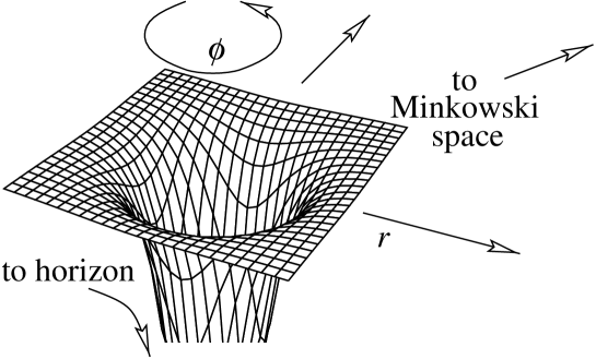
Figure 1.1: A cross section of the metric (1.9) in the $r-\phi$ plane, where $\phi$ is the lateral polar angle in the transverse sphere. The local extrinsic curvature is an approximate representation of the curvature scale appearing in the original metric at the corresponding point in space. Far way from the center, the geometry becomes flat.

By standard techniques of general relativity, one can calculate the entropy of (1.9), as well as its energy content as measured by an observer at infinity. The reader is referred to Appendix A for some of the technical details regarding such computations. We find that the equation of state for the thermodynamic state comprised of $N$ non-extremal Dp branes is given by [14, 21, 22]

$$E\sim\left(\frac{S^{2}}{N}\right)^{\frac{7-p}{9-p}}\left(\frac{\Sigma^{p(p-5)}g_{\it str}^{3-p}}{{\alpha^{\prime}}^{\frac{(p-3)^{2}}{2}}}\right)^{\frac{1}{9-p}}\ .$$ (1.13)

Here $E$ is the energy measured above the mass of the extremal branes, and $S$ is the entropy. The specific heat for this geometry is positive for $p<6$. The system is metastable in the sense that it evaporates slowly through Hawking radiation.

The solution given in (1.9)-(1.11) is a faithful description of the Dp branes for regions of space where the local curvature scale is small relative to the string scale, and the string coupling $g_{s}e^{\phi}<1$. Elsewhere, the original Lagrangian is corrected by new physics of string theoretical origin. Particularly, the size of these two observables, curvature and coupling, as measured at the horizon $r=r_{0}$ determine the window of validity of the equation of state (1.13), since the latter is a statement extracted from geometrical information at the horizon. These two restrictions are found to be

$$\left(g_{\it str}^{-1}\left(\frac{\Sigma^{2}}{{\alpha^{\prime}}}\right)^{\frac{p-3}{2}}\right)^{p(p-7)}<\left(N^{8-p}S^{p-7}\right)^{p-3}\ ,$$ (1.14)

for the condition $g_{s}e^{\phi}|_{hor}<1$, and

$$g_{\it str}^{p}\left(\frac{\Sigma^{2}}{{\alpha^{\prime}}}\right)^{p\frac{3-p}{2}}>S^{3-p}N^{p-6}\ ,$$ (1.15)

for the curvature scale at the horizon to be small with respect to $1/{\alpha^{\prime}}$; we will refer to this latter criterion as the Horowitz-Polchinski correspondence point. We thus have a gravitational description of the thermodynamic state of $N$ excited Dp branes for certain entropies $S$, asymptotic string coupling $g_{\it str}$, and torus size $\Sigma$.

1.4 Open strings and Yang-Mills theories

We concluded the previous section by describing Dp branes as seen by the low energy dynamics of closed string theory. In this section, we focus on Dp brane physics as emerging from the dynamics of the open strings propagating on their surfaces.

As in the closed string sector, open string dynamics is simplified by studying the low energy regime, truncating away the degrees of freedom associated with the vibrational modes of the open strings. This is again a quantum field theory of massless fields, quanta corresponding to the ground states of the open string spectrum. It is not however a gravitational theory. We further restrict to the regime where the interactions of these quanta with the gravitational closed string sector in the geometry projected by the Dp branes is negligible; this is achieved by requiring that the gravitational coupling is small. For $N$ Dp branes, the resulting theory is the dimensional reduction of ${\cal N}=1$ $U(N)$ ten dimensional Super Yang Mills (SYM) theory to the $p+1$ dimensional world-volume of the $N$ branes [17, 23, 24]

$$S=-\frac{1}{4g_{Y}^{2}}\int\ d^{p+1}y\ \mbox{Tr}\left(F_{\mu\nu}^{2}+2D_{\mu}X_{i}D^{\mu}X^{i}-[X_{i},X_{j}]^{2}\right)$$

$$+2i\mbox{Tr}\left(\overline{\lambda}\Gamma^{\mu}D_{\mu}\lambda+i\overline{\lambda}\Gamma^{i}[X_{i},\lambda]\right)\ .$$ (1.16)

All fields are $N\times N$ hermitian matrices in the adjoint of $U(N)$. Throughout this thesis, we will assume that $N\gg 1$ for reasons that will become evident in the next Chapter. $D_{\mu}\equiv\partial_{\mu}-i[A_{\mu},\ ]$ is the standard covariant derivative. We have the gauge field strength $F_{\mu\nu}$, where $\mu,\nu$ run over the $p+1$ coordinates parameterizing the world-volume of the Dp branes; the scalars $X^{i}$, where $i$ runs over the space dimensions transverse to the branes; and the sixteen “gaugino” field $\lambda^{\alpha}$ as Majorana Weyl spinors of $SO(9,1)$. The Yang-Mills coupling $g_{Y}$ is given by

$$g_{Y}^{2}=(2\pi)^{p-2}g_{\it str}{\alpha^{\prime}}^{\frac{p-3}{2}}\ .$$ (1.17)

We will also take the coordinates $y_{\mu}$ that parameterize the world-volume of the branes to live on a torus with cycle circumferences equal to $\Sigma$, i.e. the Dp branes are wrapped on a torus of size $\Sigma$.

An intuitive insight can be obtained as to the meaning of the scalar fields in the SYM action as follows. Expanding around a background consisting of diagonal scalar matrices $X^{i}$, $g_{Y}^{2}$ is found to tune the masses of the off-diagonal modes of the scalar matrices. For the branes separated from each other by super-Planckian distances, the diagonal elements of these matrices can be thought of as representing the positions of the $N$ branes in the transverse space to their worldvolumes. The massive off-diagonal elements may then be integrated out in an adiabatic approximation scheme to yield an effective description of the dynamics of the diagonals. Remarkably, the resulting potential between the diagonal modes is found to be of gravitational character. This is suggesting that closed string physics and space-time are encoded in the low energy open string dynamics. For sub-Planckian brane separations, this natural division of roles between diagonal and off-diagonal matrix elements cannot be made. The physics is more complex, and our intuitive picture of a smooth fabric for space falters. Suggestions have been made that this is indicative of a non-commutative structure of space-time at the eleven dimensional Planck scale.

The action (1.4) receives corrections as we probe physics at string scale energies due to the effect of the stringy vibrational modes of the open strings. Interactions with the closed string sector further alter the dynamics. Processes involving closed strings from the surrounding bulk space breaking on the surface of the branes, and open strings evaporating to closed strings, are tuned by the strength of the gravitational coupling. The action (1.4) however becomes progressively better reflection of the correct Dp brane physics in the limit

$${\alpha^{\prime}}\rightarrow 0\ \ \mbox{with}\ \ g_{Y}^{2},\ \Sigma,\ E\ \mbox{held fixed,}$$ (1.18)

henceforth referred to as the Maldacena limit. $E$ here is the energy scale of an excitation in the field theory. The gravitational coupling is given by

$${2\kappa_{10}^{2}}\sim g_{Y}^{4}{\alpha^{\prime}}^{7-p}\rightarrow 0\ \ \mbox{for $p<7$}\ .$$ (1.19)

However, we need to be careful before we conclude that all is well for $p<7$. This is because equation (1.17) implies that in the Maldacena limit $g_{\it str}\rightarrow\infty$ for $p>3$. This means that, for $p$ odd, we need to look at the S dual picture; for $p$ even, we need to look at the gravitational coupling in eleven dimensions. As discussed in Appendix B, equation (1.19) is invariant under S and T duality transformations. Hence, we only have to look at the $p=4$ and $p=6$ cases more carefully. For $p$ even and $p>3$, the eleven dimensional M theory gravitational coupling is

$${2\kappa_{11}^{2}}\sim{2\kappa_{10}^{2}}R_{11}\sim\left(g_{Y}^{2}{\alpha^{\prime}}^{\frac{6-p}{2}}\right)^{3}\rightarrow 0\ \ \mbox{for $p<6$.}$$ (1.20)

Combining these observations, we conclude that, for $p<6$ and in the Maldacena limit (1.18), both gravitational and stringy effects are scaled out, while the parameters of the field theory are held fixed. This statement defines a certain regime of energy and string coupling of interest from the perspective of our field theory.

We define the effective dimensionless coupling at large $N$, with ’t Hooft-like scaling, by

$$g_{\rm eff}^{2}\equiv g_{Y}^{2}NT^{p-3},$$ (1.21)

where $T$ is the substringy energy scale at which we study a given process with the action (1.4). We see three different scenarios arising as a function of $p$ that need to be distinguished:

• For $p<3$, the theory is super-renormalizable and well defined in the UV . The effective Yang-Mills coupling increases at low energies.

• For $p=3$, we have $3+1$d ${\cal N}=4$ SYM theory. This is a superconformal theory; its beta function vanishes.

• For $3<p<6$, the Yang-Mills coupling is irrelevant; it blows up at high energies, indicating an ill-defined theory at small length scales. A non-renormalizable theory arising at low energies may be thought of as a descendent from an otherwise more elaborate but well-defined theory in the UV; at higher energies, the degrees of freedom of the UV theory set in and regularize the dynamics. It is believed that the SYM theories for $3<p<6$ are connected in the UV to theories describing the dynamics of the NS5 branes of string theory. These connections will be tackled at slightly greater length in Section 1.5.

• For $6\leq p\leq 9$, the situation is more complicated. As we saw above, the gravitational coupling does not vanish indicating that the closed string sector does not decouple from the open string dynamics. Except for $p=6$, these cases will be omitted from the discussion in this thesis.

Consider exciting a gas of quanta in these SYM theories. The variable $T$ in equation (1.21) denotes then the temperature. For $g_{\rm eff}\ll 1$, we have a weakly interacting gas of bosons and fermions. As discussed in the Introduction, the equation of state of the finite temperature vacuum in this regime is given by equation (1.2). Perturbation theory can be applied to refine this free gas picture. As the temperature is tuned past $g_{\rm eff}\sim 1$, our understanding of the dynamics via standard field theoretical means breaks down. The physics of the theory beyond this point is then a mystery. A mystery, that is, until the advent of Maldacena’s conjecture.

1.5 Comments on five brane theories

We observed in the previous section that $p+1$ dimensional SYM theories for $3<p<6$ are non-renormalizable; i.e. they are low energy effective descriptions of physics of possibly different character that is well defined at short length scales. This UV physics can be unraveled by making use of some of the special symmetries arising in string theories. Particularly, it is known that certain duality transformations of string theories shuffle D4 branes with M5 branes, D5 branes with NS5 branes, and NS5 branes with M5 branes (see Appendix B). This suggests that $4+1$d and $5+1$d SYM theories may connect in the UV with theories describing the dynamics of five-branes. These theories are not very well understood; we will try to outline in this section a few facts known about them  [25, 26, 27, 28, 29].

We remind the reader that the NS5 brane is a five dimensional extended object that arises in string theories as the magnetic dual of the F1 string. Its dynamics appears to be fundamentally different from that of Dp branes. In particular, one does not have a picture of open strings propagating on the NS5 brane surface describing ripples of excitations. There exists however a less understood picture of closed strings living in the $5+1$d world-volume of the NS5 brane; their dynamics is presumably describing the fluctuations of the brane. This “little closed string theory” is not gravitational and is necessarily a non-local theory.

There are two flavors of NS5 branes; the one in IIA theory and the one in IIB theory, related to each other by T duality transformations. The NS5 brane of the IIA theory (NS5A) descends from the M theory five brane, the magnetic dual of the M theory membrane. The 6d string theory on its surface has $(2,0)$ supersymmetry with sixteen supersymmetry generators. Compactifying this theory on a substringy circle (i.e. wrapping the NS5A on the circle) yields $4+1$d SYM theory. The uncompactified theory appears at low energies and for well-separated branes as a $5+1$d field theory of free massless fields forming a tensor multiplet of supersymmetry. The bosonic field content of this theory is given by five scalars and an anti-selfdual two-form. The tension of the little strings is set by the tension of a membrane wrapping the M theory circle and ending on the five brane. We will see that it is held fixed in the Maldacena limit, signaling that the infinite tower of little string vibrational modes does not decouple in the energy regime of interest; this signals that we will be dealing with non-local theories arising in the UV of certain local SYM theories. The NS5 brane of the IIB theory (NS5B) is a 6d $(1,1)$ conformal field theory related to the $(2,0)$ theory by an odd number of T dualities. At low energies, it is described by $5+1$d SYM theory.

Figure 1.2 is a schematic diagram summarizing our comments in this section.

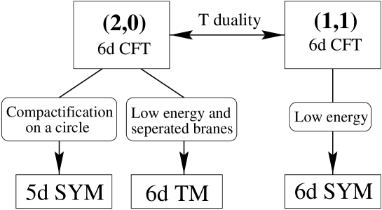
Figure 1.2: Five brane theories and their connections to various quantum field theories; TM stands for Tensor Multiplet .

When we will be studying the thermodynamics of $4+1$d and $5+1$d SYM theories, it will be appropriate to label the discussion as an analysis of the thermodynamics of five brane theories.

1.6 Maldacena’s conjecture

In the previous sections, we outlined two different descriptions for a configuration of excited Dp branes. One is through gravity, a picture consisting of a space-time curved by the energy content of the branes; the other is through the finite temperature vacuum of a non-gravitational SYM or little string theory. In the Maldacena limit, which defines a certain low energy regime, the latter picture is in focus. There are two questions that arise after these observations. First, what does Maldacena’s energy regime correspond to in the geometrical picture? And second, how does this energy regime relate to the one encountered on the geometry side in equations (1.13),  (1.14) and  (1.15)?

Consider perturbations propagating in the extremal background geometry given by the metric (1.9) with $r_{0}=0$. We may for example consider excitations in the supergravity fields, or stringy modes beyond the supergravity multiplet. The background geometry typically enforces a dispersion relation relating the energy of the perturbation as measured by an observer at infinity and the region of the background geometry where the field of the perturbation is predominantly supported. Consider for instance exciting the extremal state by knocking out one of the $N$ Dp branes of the bound system away from $r=0$. A measure of the energy of this excitation can be obtained by taking a snapshot of projected Dp brane at its maximum radial extent $r$ from the rest of the system. In the SYM, this corresponds to giving a pronounced vev to a diagonal entry in the scalar matrices. On the geometry side, we have a string radially stretched from the extremal zero area horizon at $r=0$ to a coordinate distance $r$ away. Using the metric (1.9), one finds that the energy of this stretched string as measured at infinity is proportional to $r/{\alpha^{\prime}}$. If we identify this with the energy of the excitation in the field theory, we see that that lower energy excitations tend to sit closer to the center of the geometry. Crudely put, the higher the energy of a perturbation of the extremal state, the farther is the extent in the transverse space of the “jet” or ripple produced on the Dp branes. The Maldacena energy regime (1.18) then corresponds to focusing on physics near the core of the Dp brane geometry. Equation (1.18) essentially establishes a UV cutoff on the open string theory, and corresponds to restricting dynamics in the closed string sector to the background geometry of the near horizon region of the extremal Dp brane solution. This close-up geometry of the horizon that corresponds to the Maldacena energy regime (1.18) is easily obtained from the metric (1.9) by dropping the $1$ in the harmonic function $H$ of (1.12). Having made these observations, Maldacena proposed the following [10, 30]:

Maldacena’s conjecture: String theory in the background geometry of the near horizon region of the extremal Dp branes is encoded in the corresponding SYM theory.

By this it is meant that the partition functions given by the two pictures are equal. The conjecture suggests a one to one correspondence between excitations of the background geometry and excitations in the SYM quantum field theory. This is essentially an equivalence between closed string theory (the gravitational side) and open string theory (the SYM side). Note that one is to truncate the open string dynamics to the ground states, while one is to keep the infinite tower of closed string excitations propagating in the Dp brane background. This is because, in the Maldacena limit, the ratio of string scale proper energy of a perturbation in the bulk space to its energy measured at infinity (i.e. the energy in the open string sector) is finite, i.e. independent of ${\it l}_{{{\it str}}}$.

We focus on perturbations of the extremal background that form metastable configurations corresponding to the black solutions (i.e. $r_{0}\neq 0$) of equation (1.9)  [14]. This amounts to exciting the extremal Dp branes to finite temperature, and therefore corresponds to studying a certain thermodynamic phase of the SYM theory. Maldacena’s limit zooms onto physics in the near horizon region $r=r_{0}$. Our previous picture of a Dp brane projected from the core as describing an excitation of the extremal state suggests the following: in this finite temperature scenario, the horizon $r=r_{0}$ may denote, roughly, the extent in the transverse space of a halo due to a gas of ripples on the surface of the Dp branes. This observation may indicate that the standard classical procedure to analytically continue the black geometry smoothly past the horizon is not necessarily well justified. The equation of state of this phase of the SYM theory is given by equation (1.13)

$$E\sim\left(\frac{S^{2}}{N}\right)^{\frac{7-p}{9-p}}\left(\Sigma^{p(p-5)}(g_{Y}^{2})^{3-p}\right)^{\frac{1}{9-p}}\ ,$$ (1.22)

where we have written it in terms of the field theory parameters. We see that, in the Maldacena energy regime (1.18), this energy scale is kept in focus. Equation (1.22) can be trusted for a window of entropies such that the curvature scale and the dilaton measured at the horizon are small, as we saw in equations (1.14) and (1.15). In the field theory variables, these become respectively

$$\left(N^{8-p}S^{p-7}\right)^{3-p}\left(\frac{\Sigma^{p-3}}{g_{Y}^{2}}\right)^{p(p-7)}<1\ ,$$ (1.23)

and

$$g_{Y}^{2p}\Sigma^{p(3-p)}N^{6-p}>S^{3-p}\Rightarrow g_{\rm eff}>1\ .$$ (1.24)

We see that this entropy/energy window is a subset of Maldacena’s energy regime, and that the geometrical phase arises in a non-perturbative regime of the SYM theory. Within this window, the equation of state of the black geometry then describes a certain phase of the SYM theory. The conjecture implies that the analysis of the stability of such black geometries can be translated to an analysis of critical phenomema in the SYM theory.

We thus have a powerful geometrical tool to explore the thermodynamics of SYM or little string theories beyond the confines of pertubration theory. We will make use of it to systematically map out the thermodynamic phase diagrams of these theories.

1.7 The Matrix conjecture

Prior to Maldacena’s conjecture, another proposal suggested a correspondence between gravitational and SYM theories. The Matrix conjecture [9, 11] proposed that Discrete Light Cone Quantized (DLCQ) M theory on a $p$ dimensional torus is encoded in $p+1$d SYM theory. Our thermodynamic analysis will lead to a better understanding of this statement; we will conclude that the content of this conjecture is a subset of Maldacena’s proposal. We here briefly review the Matrix conjecture for future reference. The casual reader may quickely browse through this section only to get accustomed to some of the nomenclature we will make use of later.

A convenient way to summarize the Matrix theory conjecture is to say that DLCQ M-theory on $T^{p}$ with $N$ units of longitudinal momentum is a particular regime of an auxiliary ‘${\overline{\rm M}}$-theory’ which freezes the dynamics onto a subsector of that theory. Consider such an ${\overline{\rm M}}$-theory, with eleven-dimensional Planck scale $\overline{{\it l}}_{{\rm pl}}$ (which we denote (${\overline{\rm M}}$,$\overline{{\it l}}_{{\rm pl}}$)) on a $p+1$d dimensional torus of radii ${\bar{R}}_{i}$, $i=1\ldots p$, and $\bar{R}$ the ‘M-theory circle’ of reduction to type $\overline{\rm IIA}$ string theory, in the limiting regime

$$\overline{{\it l}}_{{\rm pl}}\rightarrow 0,\ \ \ \mbox{with }x\equiv\frac{\overline{{\it l}}_{{\rm pl}}^{2}}{\bar{R}}\ \ \ \mbox{and }y_{i}\equiv\frac{\overline{{\it l}}_{{\rm pl}}}{\bar{R}_{i}}\ \ \ \mbox{fixed},$$ (1.27)

and $N$ units of momentum along $\bar{R}$. It is proposed that [9, 11]

• This theory is equivalent to an ($M$,${\it l}_{{\rm pl}}$) theory on the DLCQ background we denote by $D^{1,1}\times T^{p}\times{\bf R}^{9-p}$, where $D^{1,1}$ is a $1+1$ dimensional subspace compactified on a lightlike circle of radius $R_{+}$, and the torus $T^{p}$ has radii $R_{i}$ ($i=1\ldots p$). The map between the two theories is given by

  $$x=\frac{{\it l}_{{\rm pl}}^{2}}{R_{+}},\ \ \ y_{i}=\frac{{\it l}_{{\rm pl}}}{R_{i}},$$ (1.28)

  with $N$ units of momentum along $R_{+}$.

• The dynamics of the ${\overline{\rm M}}$ theory in the above limit can be described by a subset of its degrees of freedom, that of $N$ D0 branes of the $\overline{\rm IIA}$ theory.

The two propositions above, in conjunction, are referred to as the Matrix conjecture  [9, 11].

T-dualizing on the $\bar{R}_{i}$’s, we describe the D0 brane physics by the $p+1$d SYM of N D$p$ branes wrapped on the dualized torus. The dictionary needed in this process is

$$\bar{R}= ~{}\bar{g}_{s}^{\prime}{\it l}_{{{\it str}}}\ \ \ \overline{{\it l}}_{{\rm pl}}^{3}= \bar{g}_{s}^{\prime}{\it l}_{{{\it str}}}^{3}\ ,$$

$$\bar{g}_{s}= ~{}\bar{g}_{s}^{\prime}\frac{{\bar{\it l}}_{{{\it str}}}^{p}}{\Pi\bar{R}_{i}}\ \ \ \Sigma_{i}= \frac{{\bar{\it l}}_{{{\it str}}}^{2}}{\bar{R}_{i}}\ .$$ (1.29)

The first line is the ${\overline{\rm M}}-\overline{\rm IIA}$ relation, the second that of T-duality. The limit (1.27) then translates in the new variables to

$$\bar{\alpha}^{\prime}\rightarrow 0\quad,\quad\quad\mbox{with }\ \ g_{Y}^{2}=(2\pi)^{p-2}\bar{g}_{s}{{\bar{\alpha}}}^{\prime\frac{p-3}{2}}\ \ \ \mbox{and }\Sigma_{i}\ \ \ \mbox{fixed}\ ,$$ (1.30)

where the nomenclature $g_{Y}^{2}$ and $\Sigma_{i}$ refers to the coupling and radii of the corresponding $p+1$d $U(N)$ SYM theory. This is simply the Maldacena limit (1.18).

Chapter 2 A simple phase diagram

We concluded in the previous chapter that the thermodynamic state described by the Dp brane geometry given by (1.9) with equation of state (1.13) corresponds to a certain phase in the thermodynamic phase diagram of $p+1$d SYM. This is obviously a different phase than the one accesible by perturbation theory, whose equation of state scales as (1.2). In this chapter, we focus on the case of D0 branes ($p=0$), and we investigate the transition between the perturbative and geometrical phases. In the process, we will map the thermodynamic phase diagram of the $0+1$d SYM theory well into non-perturbative regimes. We will present a relatively detailed analysis since this simple case can be used to illustrate some of the basic ideas involved in the more elaborate thermodynamic phase diagrams we will encounter in the next chapter.

2.1 Thermodynamics of D0 branes

We are considering $0+1$d SYM theory which describes the dynamics of D0 branes in IIA string theory. We take the number of D0 branes $N$ to be much greater than one. The effective Yang-Mills coupling is given by equation (1.21); using equation (1.22) and $E\sim TS$ with $p$ set to zero, this yields

$$g_{\rm eff}^{2}\sim\left(\frac{N^{2}}{S}\right)^{5/3}\ ,$$ (2.1)

At entropies much greater than $N^{2}$, we see that the system is in a weakly coupled phase. We have a quantum mechanical system with $N^{2}$ weakly interacting particles propagating in an infinite volume; this is because we have not restricted the SYM scalars, the coordinates of the particles, to live within a confined region. As such, the stability of such a phase is at issue; the physics of this phase will be discussed in greater detail below. As the interactions become strong at $S\sim N^{2}$, the dynamics becomes more interesting; we expect to form a ball of strongly interacting particles that are confined to a region of space by virtue of these strong interactions. Putting the system in a box is not necessary anymore if we are content to describe metastable phases that evaporate slowly.

We lower the entropy of our system past $S\sim N^{2}$, venturing into non-perturbative dynamics $g_{\rm eff}^{2}\gg 1$. Consider the near horizon geometry of $N$ excited D0 branes given by (1.9) with $p=0$

$$ds_{10}^{2}=-H^{-1/2}hdt^{2}+H^{1/2}\left(h^{-1}dr^{2}+r^{2}d\Omega_{8}^{2}\right)\ ,$$ (2.2)

$$H\sim g_{\it str}{\it l}_{{{\it str}}}^{7}\frac{N}{r^{7}}\ .$$ (2.3)

$r_{0}$ is related to the entropy by the Hawking area law

$$r_{0}^{9}\sim g_{\it str}^{3}{\it l}_{{{\it str}}}^{9}\frac{S^{2}}{N}\ .$$ (2.4)

The equation of state is given by (1.13) with $p=0$

$$E\sim\frac{g_{\it str}^{1/3}}{{\it l}_{{{\it str}}}}\left(\frac{S^{2}}{N}\right)^{7/9}\ .$$ (2.5)

Maldacena’s conjecture states that this is a phase in $0+1$d SYM quantum mechanics. It is a long-lived, metastable thermodynamic phase that evaporates slowly by Hawking radiation. Let us next look closer to the criteria making this geometrical picture a physically consistent one. Its curvature scale is set by the angular part of the metric. We require that this scale, as measured at the horizon $r_{0}$, be less than $1/{\alpha^{\prime}}$. This yields the condition

$$\left.H^{1/2}r^{2}\right|_{r=r_{0}}>{\alpha^{\prime}}\Rightarrow S<N^{2}\ .$$ (2.6)

We see that the geometrical phase complements the perturbative regime; for $S>N^{2}$, we have the phase described by perturbation theory and for $S<N^{2}$, strongly coupled dynamics forces the system into another phase with equation of state  (2.5). The point $S\sim N^{2}$ is most likely a phase transition line, but our analysis is crude enough not to allow us to study the details of this transition. Our entire discussion in this thesis will suffer from this deficiency. We will be able to track the bulk phase structure of the phase diagrams and the rough scaling of the critical curves. We will make no attempt at going into a more detailed analysis of these critical phenomena.

The next task is to determine what happens to the strongly coupled phase as we decrease the entropy further. To answer this, we need to look at the dilaton

$$e^{\phi}=H^{3/4}\ .$$ (2.7)

As discussed in the previous chapter, consistency of the geometrical description requires us to assure that $\left.g_{\it str}e^{\phi}\right|_{r=r_{0}}\ll 1$; i.e. perturbative string theory was assumed in deriving the low energy supergravity action. This yields the condition

$$S>N^{8/7}\ .$$ (2.8)

For lower entropies, the size of the eleventh dimension of M theory is of super-Planckian size (c.f. equation (1.3)). The full eleven dimensional nature of the underlying dynamics must be taken into account. The connection between M and IIA theories at the low energy supergravity level is simply through the prescription of dimensional reduction that is commonly used in the compactification of supergravity theories. A few technical details can be found in Appendix B. The eleven dimensional metric from which our IIA metric (2.2) descends is found to be

$$ds_{11}^{2}=H(dx_{11}-dt)^{2}+dx_{11}^{2}-dt^{2}+H^{-1}(1-h)dt^{2}+h^{-1}dr^{2}+r^{2}d\Omega_{8}^{2}\ .$$ (2.9)

Here $x_{11}$ lives on a circle of size $2\pi R_{11}$, and the M theory Planck scale is denoted by ${\it l}_{{\rm pl}}$. This is simply a black wave propagating along $x_{11}$ (we label it W11 for future reference). D0 branes of IIA theory map onto gravitational waves in M theory. The equation of state is unchanged; we are describing the same physics using a new setting whose low energy dynamics we can trust beyond the perturbative string theory regime.

The question now becomes what happens to this eleven dimensional geometry as we lower the entropy further. This is answered by studying the stability of the black wave geometry. It is known that a black wave in a box is unstable toward collapse into a boosted black hole localized in the box; the transition occurs at the point where the boosted black hole has less free energy. As we lower the entropy, we cool the black wave enough that the preferred configuration is one which is localized in the box along the direction of wave propagation. Alternatively, a boosted black hole in a box can be said to smear itself into a black wave geometry as the entropy is raised past the point where the size of the horizon is the size of the box. This process is sketched in Figure 2.1.

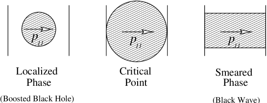
Figure 2.1: The transition between a localized boosted black hole and a black wave. The horizontal axis in these pictures is the M theory cycle of size $R_{11}$ .

The boosted black hole geometry is obtained by applying the appropriate Lorentz boost transformation on a Schwarzchild black hole (see Appendix A). The equation of state of a black hole of mass $M$ boosted to a large momentum $p_{11}=N/R_{11}=N/(g_{\it str}{\it l}_{{{\it str}}})$ is given by

$$E\sim\frac{g_{\it str}^{1/3}}{{\it l}_{{{\it str}}}}\frac{S^{16/9}}{N}\ ,$$ (2.10)

following the comments in the footnote of Section 1.7. Note that we are identifying the SYM Hamiltonian with the Light Cone energy in M theory. We can find the transition point between this phase and the black wave phase by either minimizing the Gibbs energies between (2.10) and (2.5), or by equating the size of the box $x_{11}$ as measured at the horizon to the size of the horizon. This yields the point of transition at

$$S\sim N\ .$$ (2.11)

The conclusion is that, at $S\sim N$, there is a transition between the phase described by the equation of state (2.5), and the phase of a boosted black hole described by the equation of state (2.10). For $S<N$, the $0+1$d SYM theory is in a thermodynamic state which is a boosted black hole, with the boost momentum related to the rank of the gauge group. This phase, unlike that of a stationary black hole, has positive specific heat. Figure 2.2 depicts graphically the phase diagram we have been constructing.

Figure 2.2: The thermodynamic phase diagram of $0+1$d SYM. The dotted line represents the lift to M theory. We have a total of three phases: a perturbative quantum mechanics phase, a phase of black D0 branes (comprised of two geometrical patches), and a phase of a boosted eleven dimensional black hole .

This simple example illustrates the basic idea we will make use of in the next chapter in mapping the thermodynamic phase diagrams of more elaborate cases. We use Maldacena’s conjecture to identify phases in SYM theories which have strongly coupled dynamics with Dp brane geometries; we analyze the stability and validity of these geometrical phases, using the duality symmetries if needed, and import the conclusions to SYM thermodynamics. We will be able to systematically chart in this manner the phase diagrams of SYM and little string theories on tori.

A few more comments regarding the role of the vevs of the scalars in the dynamics are in order. We saw that the perturbative $0+1$d SYM phase consists of a gas of $N^{2}$ weakly coupled particles in infinite volume. As such, its thermodynamics is well defined provided that the kinetic energy content of the zero modes of this gas is comparable to the potential energy content; we then can expect that a long lived metastable phase exists, a ball of a gas confined to a region of space by virtue of the weak interactions between the constituents. The existence of a potential strong enough to bind the zero modes is crucial in the $0+1$d case since the only dynamics available is one that can probe the infinite extent of the space. Whether a stable or metastable phase sits on the left of Figure 2.2 is then in principle left as an open issue. We focus instead on the $p+1$d SYM theories with $p\neq 0$, where this problem will be considerably milder. These cases involve the physics of Dp branes wrapped on a torus. The difference between the two scenarios is analoguous to the following more mundane situations: on the one hand, consider a gas of a certain number of particles propagating on the infinite two dimensional plane; on the other hand, consider a vibrating rubber band wrapping a cylinder. The thermodynamics of the former case is similar to the $0+1$d SYM case we discussed. In the rubber band scenario however, the physics involves in addition the thermodynamics of the vibrational modes, quanta propagating along the band (modding out the dynamics of the center of mass of the rubber band, which readily explores the longitudinal infinite extent of the cylinder). The contribution to the free energy of this sector of the dynamics dominates the thermodynamics; by increasing the temperature in the $p+1$d SYM case with $p\neq 0$, we will see that one transfers dynamics to the fluctuations on the surface of the wrapped Dp branes; this phenomena will happen at $S\sim N^{2}$. The perturbative $p+1$d SYM phases for $p\neq 0$ will be better defined in this sense; for scaling purposes, they can be readily approximated by systems of free particles living on a torus.

Typically, phases involving weakly interacting dynamics, such as the perturbative SYM gas or, more interestingly, the Matrix string, abut black geometrical phases on our phase diagrams. We expect that the vevs of the scalars in the weakly coupled phases explore the extent of the non-compact space for arbitrarily high temperatures. It is not obvious that, starting from such a phase and moving toward strongly coupled dynamics, we are guaranteed to collapse the system into one of the black geometries we encounter along the traced path. The system may have spread itself into large volumes of the transverse space (or an infinite volume in the pathological $0+1$d SYM case) such that the interactions, which generically fall in strength with distance, are effectively too weak to lead to a collapse at the point identified on the phase diagram. This phenomena will be explored in detail in Chapter 4. Our phase diagrams are faithful representation of the physics if we trace paths starting from black objects and moving toward weakly coupled phases; such paths are not necessary reversible. In Chapter 4, we map out a thermodynamic phase diagram which can be navigated with reversible processes. Note that this physics is again intimately tied with our choice not to restrict the scalar vevs to a finite region of space.

Before we conclude this chapter, let us reflect on the boosted M theory phases (the wave W11 and the black hole) that arose at low entropies. Using the M-IIA relations (1.3), we cast the Maldacena limit in the parameters of this M theory; this yields

$${\it l}_{{\rm pl}}\rightarrow 0\ \ \mbox{with}\ \ \frac{{\it l}_{{\rm pl}}^{2}}{R_{11}}\ \ \mbox{held fixed.}$$ (2.12)

We see that this is identical to the energy regime of the Matrix conjecture (1.27); i.e. the Matrix regime is a statement dual to the Maldacena limit, where the duality at play here is the M theory-IIA connection. Another map between the two limits (involving a T duality transformation) was given in the case of $p+1$d SYM with $p\neq 0$ in Section 1.7. We will see how this relation gets embedded in the phase diagrams of the next Chapter. The conclusion is the same: the Maldacena and Matrix energy regimes are dual to each other. The low entropy phases of our diagrams live in DLCQ M theory. The charge $N$ carried by the D0 branes is mapped onto the momentum in the Light-Cone direction. In this sense, Maldacena’s conjecture leads to the Matrix proposal.

Given the elaborate web of dualities between the various string theories that connect vacua of the underlying theory, a conjecture relating a field theory to string theory in a given background vacuum is naturally extended to a statement relating this field theory to string/M theory on any dual background. Given that one typically needs to accord a window of energy or of the thermodynamic parameter space to a given background vacuum, the field theory encodes naturally string/M theory in different backgrounds for different regimes of energy or temperature. A thermodynamic phase diagram constructed in this manner paints a global picture of the thermodynamic vacuum of a single theory; the role of the web of dualities in patching various string theories into one big theory metamorphoses into the role of combining various thermodynamical vacua of a single SYM theory into a single phase diagram. We see in the $0+1$d SYM phase diagram a very simple realization of these ideas.

2.2 The Matrix black hole

We saw in the previous sections that a boosted black hole, or a black hole in DLCQ M theory, is a thermodynamic phase of $0+1$d SYM theory. We will find it a generic phase arising at low entropies in $p+1$d SYM theories with $p\leq 6$. The question then arises as to how this phase is realized as excitations of the SYM fields at fixed temperature or entropy. A model for this was proposed in [32, 33, 34] which we now summarize.

At low entropies $S<N$, consider the scenario where the SYM dynamics is dominated by that of the zero modes of the fields with the effective Yang-Mills coupling being large. Assuming that the diagonal elements of the scalars $X^{i}$ do not take degenerate values, the off-diagonal modes are massive with the mass scale tuned by the Yang-Mills coupling. For large coupling, these degrees of freedom can be integrated out to yield an effective low energy potential between the diagonal elements. The latter represent, as discussed earlier, the coordinates of $N$ D0 branes, each with mass $1/R_{11}$ (c.f. equations (1.3) and (1.7)). So, we have a gas of $N$ D0 branes interacting with some effective potential. It is proposed that, for $S<N$, there is a stable thermodynamic state in the SYM that can be modelled as a gas of $K$ clusters of D0 branes, each with $N/K$ D0 branes. It is assumed that the physics of this model is dominated by the center of mass dynamics of these clusters of D0 branes. The clustering phenomena of the D0 branes into nuclei with $N/K$ partons is in principle an unknown, an assumption that will be justified in the analysis of Chapter 4. The scaling of the kinetic energy content of this gas can be read off the Langangian 1.4

$${\cal K}\sim KM_{clst}v^{2}\sim K\left(\frac{N}{KR_{11}}\right)v^{2}\ ,$$ (2.13)

where $v$ is the velocity of a cluster. The potential energy content of the gas due to the interactions between two clusters is found to be

$${\cal V}\sim\frac{\kappa_{11-p}^{2}}{R_{11}}\frac{N}{K}\frac{\left(M_{clst}v^{2}\right)^{2}}{r^{7-p}}\sim\frac{{\it l}_{{\rm pl}}^{9}}{R_{11}R^{p}}\left(\frac{N}{K}\right)\left(\frac{N}{KR_{11}}v^{2}\right)^{2}\frac{1}{r^{7-p}}\ ,$$ (2.14)

where $r$ is the typical seperation between the clusters, or the size of the system. We are considering a boosted black hole in M theory on a $p$ dimensional torus $T^{p}$ of equal cycle sizes $R$; this changes the gravitational coupling and the power of the cluster seperation distance $r$ as shown. We have also enhanced the interaction by a factor $N/K$. At this stage, this is an assumption; it will be justified in Chapter 4 and Appendix F.

We now make use of three additional ingredients. We assume that the clusters are distinguishable from each other. We then have the entropy of the gas scaling as $S\sim K$. We assume that the wavefunctions of the clusters saturate the quantum mechanical uncertainty bound

$$p\ r\sim 1\Rightarrow\frac{N}{KR_{11}}v\ r\sim 1$$ (2.15)

Furthermore, the virial theorem dictates

$${\cal K}\sim S^{2}{\cal V}\Rightarrow r^{9-p}\sim\frac{{\it l}_{{\rm pl}}^{9}}{R^{p}}S\ .$$ (2.16)

Puting things together in equation (2.13) or (2.14), we get that the total energy for this gas scales as

$$E\sim\frac{R_{11}}{N}\left(S^{\frac{8-p}{9-p}}\left(\kappa_{11-p}^{2}\right)^{\frac{1}{p-9}}\right)^{2}\sim\frac{M^{2}}{p_{11}}\ ,$$ (2.17)

where we have assumed in the last step that the SYM Hamiltonian is the Light-Cone energy as in equation (1.25). The mass $M$ obtained in this equation, up to numerical coefficients, is that of a Schwarzchild black hole in an eleven dimensional space-time compactified on a torus $T^{p}$ of size $R$. The proposed model then reproduces black hole physics from SYM theory. Various assumptions made in constructing this model will be justified in the analysis of Chapter 4.

2.3 The Matrix string

Another phase that we will encounter in the various phase diagrams is that of the Matrix string. This is a highly excited string in DLCQ string theory with entropy $S\gg 1$. Its equation of state has the Light-Cone structure (1.25)

$$E=\frac{M^{2}}{2p_{+}}\ ,$$ (2.18)

where $M^{2}$ is the mass of a free string at a level of degeneracy $e^{S}$

$$M^{2}\sim\frac{S^{2}}{{\alpha^{\prime}}}\ .$$ (2.19)

This phase arises, for example, in the IR of $1+1$d SYM theory where a free conformal field theory is believed to sit. An explicit realization of the free string as excitations in this theory was given [35, 36]. We summarize briefly this proposal.

In the IR, the relevant Yang-Mills coupling is large; this makes the commutator terms in the action (1.4) costly in energy. Configurations where all matrix fields are diagonal are energetically favoured. Consider diagonal matrix configurations for the scalars $X^{i}$; we ignore the gauge fields on the world-sheet, even though these have interesting roles to play in the dynamics and the spectrum [37, 38, 39, 40]. Gauge transformations that permute the diagonal elements form a symmetry of this setup. In general, we need to consider boundary conditions on the scalar matrices allowing for such discrete gauge transformations

$$X^{i}(y+\Sigma)=gX^{i}(y)g^{-1}\ ,$$ (2.20)

where $g$ is an $N\times N$ matrix permuting the diagonal elements. All such matrices $g$ can be decomposed into transformations involving the operation of cycling acting on subsets of the diagonal elements. Without loss of generality, we consider $g$ as a cyclic transformation in $Z_{N}$; the boundary condition above then sews the various diagonal elements together into one ‘long string’ with world-sheet length $N\Sigma$, instead of the periodicity $\Sigma$ that one obtains from the simpler condition $X^{i}(y+\Sigma)=X^{i}(y)$. This is a basic technique known, for example, from string theory on orbifolds. The picture depicts a IIA string encoded in the IR of the $1+1$d SYM as a D string wrapping, like a ‘slinky’, $N$ times a circle which is seen as the M cycle from which the IIA string theory descends. Note that the $SO(8)$ symmetry of the scalar fields is precisely the corresponding symmetry of IIA string theory in the Light-Cone frame. It is then easy to show that the quantized Hamiltonian of (1.4) leads to the free Light-Cone string spectrum (2.18) with $p_{+}=N/R_{+}$.

The appearance of a Matrix string with $S\gg 1$ in our phase diagrams implies that there exists rich dynamics that seeds a certain ordering, a $Z_{N}$ holonomy, in the SYM excitations as we navigate past certain critical curves. The closest analogy may be a gas-solid phase transition, where the symmetries of the emerging lattice encode characteristics of the underlying microscopic dynamics. The picture of the Matrix string we outlined here will be an integral part of our discussion in Chapter 4.

Chapter 3 More Thermodynamics

3.1 Strategy

In this chapter, we investigate phase diagrams of $p+1$d SYM theories on tori for $0<p<7$; we also study the phase diagram for a system of intersecting D1 and D5 branes. Unlike the $p=0$ case, we will deal with finite size effects resulting from the torus on which the thermodynamics lives. In the D1D5 system, the role of angular momentum in criticality will be one of the new ingredients.

The basic idea is a systematic analysis of various black supergravity vacua; the underlying strategy goes as follows: A $10$D or lower-dimensional near-extremal supergravity solution must satisfy the following restrictions:

• The dilaton at the horizon must be small. Otherwise, in a IIA theory, we need to lift to an $11$D M-theory; in a IIB theory, we need to go to the S-dual geometry. This amounts to a change of description – a reshuffling of the dominant degrees of freedom – without any change in the equation of state.

• The curvature at the horizon must be smaller than the string scale. Otherwise, the dynamics of massive string modes becomes relevant. By the Horowitz-Polchinski correspondence principle [41], as in equation (1.15), a string theory description emerges – an excited string, or a perturbative SYM gas reflecting weakly coupled D-brane dynamics. This is generally associated with a change of the equation of state; in the thermodynamic limit, we may expect critical behavior associated with a phase transition. This criterion can easily be estimated for various cases when one realizes that the curvature scale is set by the horizon area divided by cycle sizes measured at the horizon; i.e. the localized horizon area should be greater than order one in string units.

• Cycles of tori on which the geometry may be wrapped, as measured at the horizon, must be greater than the string scale [42]. Otherwise, light winding modes become relevant and the T-dual vacuum describes the proper physics [43]. We expect no critical behavior in the thermodynamic limit, since the duality is merely a change of description.

• The horizon size of the geometry must be smaller than the torus cycles as measured at the horizon [44, 45]. Otherwise, the vacuum smeared on the cycles is entropically favored. We expect this to be associated with a phase transition, one due to finite size effects, and it is associated generally with a change of the equation of state. However, it is also possible that there is no such entropically favored transition by virtue of the symmetry structure of a particular smeared geometry, so we expect no change of phase. Intuitively, a system would only localize itself in a more symmetrical solution to minimize free energy. We saw a manifestation of this transition mechanism already in the D0 phase diagram, where the black wave W11 smeared along the longitudinal direction localized into a boosted black hole (see Figure 2.1). In addition to this longitudinal localization transition, this phenomena is now to appear in the context of localization along the transverse compactified dimensions.

On the other hand, given an $11$D supergravity vacuum, a somewhat different set of restrictions applies:

• The curvature near the horizon must be smaller than the Planck scale. By the criterion outlined above, we see that, for unsmeared geometries, this is simply the statement that $S>1$; i.e. quantum gravity effects are relevant for low entropies. For large enough longitudinal momentum $N$, this region of the phase diagram is well away from the region of interest. This is one of the reasons for taking throughout this thesis $N\gg 1$.

• The size of cycles of the torus as measured at the horizon must be greater than the Planck scale. Otherwise, we need to go to the IIA solution descending from dimensional reduction on a small cycle. We expect no change of equation of state or critical behavior.

• The size of the M-theory cycles, including the Light-Cone longitudinal box, as measured at the horizon, must be bigger than the horizon size. Otherwise, the geometry gets smeared along the small cycles. This is expected to be a phase transition due to finite size physics.

Applying these criteria, we then select the near extremal geometry dual to a phase in SYM theory on the torus, and navigate the phase diagram via duality transformations suggested by the various restrictions. We will then be charting the phase diagram of SYM quantum field theories or little string theories. Alternatively, we are tracing through the phases visited by a DLCQ M theory black hole, the latter being a phase that arises on all our diagrams for low entropies; the Schwarzchild black hole being a generic state in M theory, we may propose that we are mapping the thermodynamic phase diagram of DLCQ M theory.

We will avoid presenting the calculations that lead to the construction of the upcoming phase diagrams. The details can be found in [3, 4]. The basic idea was illustrated in the previous chapter. Further background material needed to decode the physics of the phase diagrams can be found in Appendix B. The details of the scaling of the various transition curves and the equations of state of the bulk phases for all our phase diagrams are tabulated in Appendix C. Note also that the structure of all the diagrams can be checked by minimizing the Gibbs energies between the various phases.

3.2 Phase diagrams of Super Yang-Mills on tori

The phase diagrams for Dp branes on tori have a number of common features. We focus on these aspects first; the reader is referred to, for example, Figure 3.1 throughout the first part of this discussion. The vertical axis of the diagrams will be entropy; for the horizontal axis we take the size $V$ of cycles on the torus $T^{p}$, in eleven dimensional Planck units, as measured in the Light-Cone M-theory phase appearing in the lower right corner (the phase of boosted 11d black holes). $N$ is the charge carried by the system: brane number in the high entropy regimes and longitudinal momentum in the low-energy, Light-Cone M-theory phase. The SYM torus radii $\Sigma$ and the effective SYM coupling for large $N$ can be written in terms of the parameters of the boosted black hole phase

$$\Sigma=\frac{{\it l}_{{\rm pl}}^{2}}{R_{11}V}\quad,\qquad g_{\rm eff}^{2}\sim g_{Y}^{2}NT^{p-3}\sim V^{-p}N\left(\frac{T{\it l}_{{\rm pl}}^{2}}{R_{11}}\right)^{p-3}$$ (3.1)

($T\sim E/S$ is the temperature). The unshaded areas are described by various supergravity solutions, while the shaded regions do not have dual geometrical descriptions. Throughout the various phases, the corresponding gravitational couplings vanish in the Maldacena limit (except for $p=6$, where the limit keeps the Planck scale of the high-entropy phase held fixed), implying the decoupling of gravity for the dual dynamics. Solid lines on the diagrams denote thermodynamic transitions separating distinct phases, while dotted lines represent symmetry transformations which change the appropriate low-energy description. We do not expect sharp phase transitions along these dotted curves since the scaling of the equations of state is unchanged across them. This, does not in principle exclude the possibility of smoother (i.e. higher order) transitions.

The structure of the phase diagram for $V>1$ is identical in all the cases we encounter. At high entropies and large M theory torus, we have a perturbative p+1d SYM gas phase. Its Yang-Mills coupling $g_{Y}$ increases toward the left. The effective dimensionless coupling is of order one on the double lines bounding this phase, which are Horowitz-Polchinski correspondence curves. As the entropy decreases at large $V$, there is a D0 brane phase arising at $S\sim N^{2}$ on the right and middle of the diagrams. From the perturbative SYM side, this is where the thermal wavelength becomes of order the size of the box dual to $V$, $T_{c}\sim\Sigma^{-1}$; from the D0 phase side, it is a Horowitz-Polchinski correspondence curve. This transition may be associated with rich microscopic physics. From the thermodynamic perspective, as the transition is crossed, dynamics is transferred from local excitations in $p+1$d SYM to that of its zero modes; and Dp brane charge of the perturbative SYM is traded for longitudinal momentum charge of Light-Cone M-theory. This process is one of several paths on the phase diagram relating the Maldacena and Matrix conjectures.

The description of the D0 phase within strongly coupled SYM theory would be highly interesting. We see that this phase localizes into a Light-Cone 11d black hole phase for entropies $S<N$. This region of the phase diagram is then a reproduction of Figure 2.2; i.e. for $V\rightarrow\infty\Rightarrow\Sigma\rightarrow 0$, we connect to the $0+1$d SYM physics. The line $S\sim N$ separates the 11d phases that are localized on the M-theory circle (whose coordinate size is $R_{11}$) from those that are delocalized, uniformly across the diagram  [46, 33, 32, 47]. The 11d black hole phase at small entropy becomes smeared across the $T^{p}$ when the horizon size becomes smaller than the torus scale $V$; we denote generally such smeared phases by an overline (in this case $\overline{11D}$). This (de)localization transition of the horizon on the compact space extends above the $S\sim N$ transition, separating the black Dp brane phase from the black $D0$ brane phase. Initially, the $D0$ brane phase becomes smeared to $\overline{D0}$; as the entropy increases, the effective geometry of the latter patch becomes substringy at the horizon, and one should T-dualize into the black Dp brane patch. Both the $\overline{D0}$ and $Dp$ patches have the same equation of state, since they are related by a symmetry transformation of the theory; they are different pieces of the same phase. The localization transition line runs into the correspondence curve separating the SYM gas phase from the geometrical phases at $S\sim N^{2}$. Thus as we move to the left (decreasing $V$, i.e. increasing bare SYM coupling) at high entropy $S>N^{2}$, the SYM gas phase reaches a correspondence point; on the other side of the transition is the phase of black Dp-branes.

A further common feature of the diagrams is a ‘self-duality’ point at

$$V\sim 1\ \ \mbox{and}\ \ S\sim N^{\frac{8-p}{7-p}}\ ,$$ (3.2)

where a number of U-duality curves meet. That the various patches do not overlap is a self-consistency check on the logical structure of the picture. Basically, there is always only one set of degrees of freedom that dictate the low energy dynamics in a given window of the thermodynamic parameter space.The duality transformation that patch the various string theories together now mold various thermodynamical vacua into one phase diagram for the SYM theory. We also note the following connections to previous work. For high entropies, localization effects are circumvented and the phases are the ones studied in [14]; the triple point on the upper right corner was the one studied in [42].

On the diagram, the behavior of the effective SYM coupling depends on the equation of state governing a given region under consideration. We find the equipotentials of the effective coupling in the Dp phase

$$g_{\rm eff}^{2}\sim\left(N^{6-p}S^{p-3}V^{-3p}\right)^{\frac{5-p}{9-p}}\ .$$ (3.3)

For $p<4$ and in the Dp phase domain, the effective coupling increases diagonally on the diagrams as we move toward lower entropies and smaller volumes $V^{p}$. Using the equation of state of the localized D0 phase, we obtain the equipotentials in the D0 phase for all diagrams

$$g_{\rm eff}^{2}\sim\left(\frac{N^{2}}{S}\right)^{5/3}\ ,$$ (3.4)

i.e. equation (2.1). The coupling increases from one at $S\sim N^{2}$ as we lower the entropy toward the $11$D black hole phase. From SYM physics, both correspondence curves are where the effective coupling is of order one; the localization effect at $S\sim N^{2}$ changes this effective coupling appropriately.

In contrast, the structure of the phase diagrams for $V<1$ depends very much on the specific case at hand. The $p=1,2,3$ diagrams will be displayed and discussed next. The $p=4,5,6$ cases will be tackled in the next section.

Figure 3.1 depicts the thermodynamic phase diagram of SYM theory

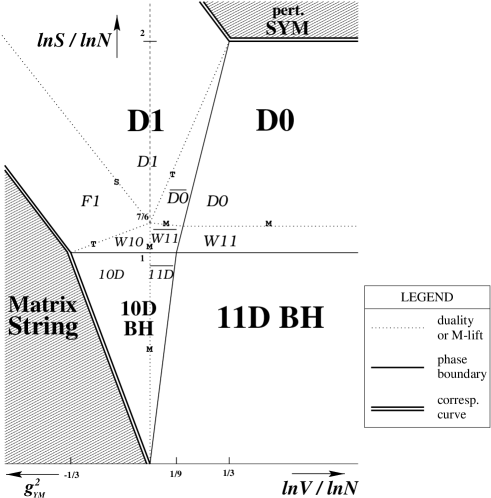
Figure 3.1: Phase diagram of SYM theory on $T^{1}$; $S$ is entropy, $V$ is the radius of the circle in Planck units, $N$ is the longitudinal momentum. The geometry label dictionary is as follows: D0: black D0; $\overline{D0}$: black D0 smeared on $V$; D1: black D1; F1: black IIB string; W10: black IIA wave; W11: $11$D black wave; $\overline{W11}$: $11$D black wave smeared on $V$; $10$D BH: IIA Light-Cone black hole; $11$D BH: Light-Cone M-theory black hole; $\overline{11D}$ BH: Light-Cone M-theory BH smeared on $V$. $M$, $T$ and $S$ stand for respectively an M-duality (such as reduction, lift or M flip on $T^{3}$), a T-duality curve, and an S duality transition.

on the circle. In total, we have six different thermodynamic phases. The salient feature of this diagram is the Matrix string phase, characterized by $Z_{N}$ order, appearing in the IR of the SYM on the left and at strong coupling. This phase is an interesting platform to explore some of the phase transitions through a statistical mechanical setting. Note that the dynamics is such that the Matrix string will emerge from the adjacent black geometrical phases as we move toward the left of the diagram; this path is however not reversible as discussed earlier. The physics of this phenomena will be explored in Chapter 4 in detail.

Figure 3.2: Phase diagram of SYM theory on $T^{2}$. The geometry label dictionary is as follows: D0: black D0; $\overline{D0}$: black D0 smeared on $V$; D2: black D2; M2: black membrane; $\overline{M2}$: black membrane smeared on a dual circle; WB: black IIB wave; $\overline{WB}$: black IIB wave smeared on a dual circle; W11: $11$D black wave; $\overline{W11}$: $11$D black wave smeared on $V$; $11$D BH: Light-Cone M-theory black hole; $\overline{11D}$ BH: Light-Cone M-theory black hole smeared on $V$; $10$D BH: IIB Light-Cone black hole; $\overline{10D}$ BH: IIB Light-Cone black hole smeared on a dual circle.

Figures (3.2) and (3.3) depict the phase diagrams

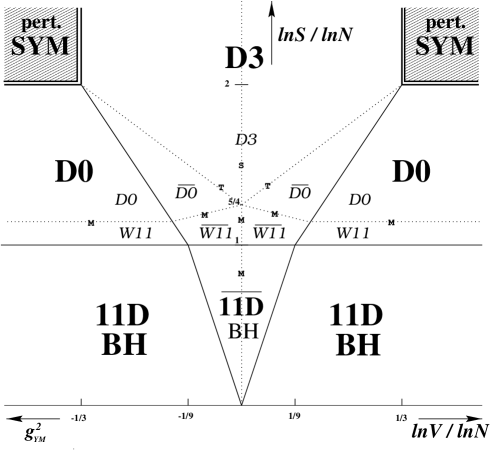
Figure 3.3: Phase diagram of SYM theory on $T^{3}$. D0: black D0; $\overline{D0}$: black D0 smeared on $V$; D3: black D3; W11: $11$D black wave; $\overline{W11}$: $11$D black wave smeared on $V$; $11$D BH: Light-Cone M-theory black hole; $\overline{11D}$ BH: Light-Cone M-theory black hole smeared on $V$.

for SYM theory on $T^{2}$ and $T^{3}$; $V$ here is again the radius of the cycles (which are chosen to be equal) measured in Planck units. In the strong coupling region of SYM on $T^{2}$, the SYM dynamics approaches the infrared fixed point governing the dynamics of M2 branes – the conformal field theory dual to M-theory on $AdS_{4}\times S^{7}$ (in ‘Poincare’ coordinates). The proper size of the $T^{2}$ shrinks toward the origin; at high entropy, the black M2 geometry accurately describes the low-energy physics, while at low entropy the near-horizon geometry is best described in terms of the IIB theory dual to M-theory on $T^{2}$ [48]. In the $T^{3}$ case, the diagram reflects the self-duality of the D3 branes and M-theory on $T^{3}$ as reflection symmetry about $V\sim 1$. The ’t Hooft scaling limit, $g_{Y}^{2}N$ fixed with $N\rightarrow\infty$, focusses in on the neighborhood of the vertical line at $\ln\,V/\ln\,N\rightarrow\pm\frac{1}{3}$.

Finally, we conclude by restating a previous observation. Starting with a thermodynamic phase in Light-Cone M-theory, say for example the lower right corner phase of the $11$D boosted black hole, using geometrical considerations, the duality symmetries of M-theory, and the Horowitz-Polchinski correspondence with the perturbative SYM phase, we would be led to conclude that Light-Cone M-theory thermodynamics is encoded in the thermodynamics of SYM QFT. We saw that the DLCQ limit is dual to the Maldacena energy regime; this mapping is depicted on the phase diagrams by the two dotted curves on the right half of the figures converging to the self-duality point. Maldacena’s conjecture asserts that underlying all these phases is super Yang-Mills theory in various regimes of its parameter space. Having not known the Matrix conjecture, we would then have been led to it from Maldacena’s proposal. The Matrix conjecture is a special realization of the more general statement of Maldacena. Correspondingly, our ability to discover the low-energy theories that yield Matrix theory on some background depends on our ability to understand duality structures with less supersymmetry in sufficient detail to construct the phase diagram analogous to figures 3.1-3.3.

3.3 Phase diagrams of Five Brane Theories

In this section, we extend our analysis to $p+1$d SYM theories for $p=4,5$, where the relevant theories involve the dynamics of five-branes [49, 29, 31, 50]; and $p=6$, where the decoupling issue is problematic [31, 50, 51, 52, 53]. In the process of generating the phase diagrams, we will rediscover the known prescriptions for generating Matrix theory compactifications on $T^{4}$, $T^{5}$, and $T^{4}/Z_{2}$; we will also comment on the difficulties encountered for $p=6$.

In addition, we will analyze the phase diagram of the D1D5 system, which arises in diverse contexts:

• It has played a central role in our understanding of black hole thermodynamics [5];

• It is a prime example of Maldacena’s conjecture, due to the rich algebraic structure of 1+1d superconformal theories which are proposed duals to string theory on $AdS_{3}\times S^{3}\times{\cal M}_{4}$ [10, 54, 55, 56];

• It describes the little string theory of fivebranes  [29, 27], where the little strings carry both winding and momentum charges.

• It is related to the DLCQ description of fivebrane dynamics [57, 58, 59, 60].

The analysis will clarify the relation of the D-brane description of the system to one in terms of NS fivebranes and fundamental strings [56], as low-energy descriptions of different regions of the phase diagram (for earlier work, see [61]).

3.3.1 Phase diagrams for $T^{4}$, $T^{5}$, and $T^{6}$

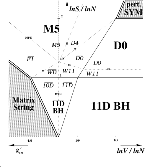
Figure 3.4: Phase diagram of the six-dimensional $(2,0)$ theory on $T^{4}\times S^{1}$. $V=R/{\it l}_{{\rm pl}}$ is the size of a cycle on the $T^{4}$ of light-cone M theory. The dashed line is the extension of the axis $V=1$, and is merely included to help guide the eye. The label dictionary is as follows: $D0$: black D0 geometry; $W11$: black 11D wave geometry; $11DBH$: 11D Light-Cone black hole; $\overline{D0}$: black smeared D0 geometry; $\overline{W11}$: black smeared 11D wave geometry; $\overline{11D}BH$: 11D smeared Light-Cone black hole; $D4$: black D4 geometry; $M5$: black M5 geometry; $\overline{F1}$: black smeared fundamental string geometry; $\overline{WB}$: black smeared IIB wave geometry; $\overline{10D}BH$: IIB boosted black hole. The phase diagram can also be considered that of the $(2,0)$ theory on $T^{4}/Z_{2}\times S^{1}$ by reinterpreting the $\overline{F1}$, $\overline{WB}$, $\overline{10D}$ phases, and the Matrix string phase as those of a Heterotic theory. .

Figure 3.4 is the phase diagram of $T^{4}$ compactification. There are six different phases, several of which – the 11d and $\overline{11d}$ black hole, black $D0$ and $Dp$ brane, and SYM gas phases – were discussed above. In a slight shift of emphasis, we have relabeled the black $D4$ brane phase as the black $M5$ brane phase, since its description in terms of the latter object extends to the region $V<1$ (in fact, even for a patch of $V>1$ the D4 brane becomes strongly coupled and must be lifted to M-theory). The appropriate dual non-gravitational description involves the six-dimensional $(2,0)$ theory on $T^{4}\times S^{1}$, where the last factor is the M-theory circle; the scale of Kaluza-Klein excitations given by the size of this circle (times the number of branes) sets the transition point between the $(2,0)$ and SYM descriptions. This $M5$ phase consists of six patches that we cycle through via duality transformations required to maintain a valid low-energy description. The energy per entropy increases toward the left and toward higher entropies; this is to be contrasted with the cases analyzed above where the IR limit appears toward the left of the diagrams. This behavior is a consequence of the reversal of the direction of RG flow between $p<3$ and $p>3$. As we continue to the left and/or down on the figure at small volume $V<1$, the $T^{4}$ is small while the M-theory circle remains large; eventually one reduces to string theory along the cycles of the $T^{4}$, and the M5-brane dualizes into a string. Somewhat further in this direction, we encounter a Horowitz-Polchinski correspondence curve, and a transition to a phase consisting of a Matrix String [35, 36, 62] with effective string tension set by the adjacent geometries. Using Maldacena’s conjecture, we thus validate earlier suggestions to describe Matrix strings using the $(2,0)$ theory [49, 29, 31]. This Matrix string phase has a correspondence curve also for low entropies, now with respect to a phase of smeared Light-Cone M theory black holes (or equivalently boosted IIB holes).

Figure 3.4 is trivially modified to give the phase diagram of the $(2,0)$ theory on $T^{4}/Z_{2}\times S^{1}$. The additional structure does not affect the critical behavior of the diagram. The change appears in the chain of dualities we perform on the dotted lines of the diagram. Appendix D contains the details. The orbifold quotient metamorphoses into world-sheet parity, and the fundamental string patch (labeled $\overline{F1}$) becomes that of the Heterotic string. The emerging Matrix string phase at the correspondence point is then that of a Heterotic theory. We thus confirm the suggestion [63, 64] to describe Heterotic Matrix strings via the $(2,0)$ theory on $T^{4}/Z_{2}\times S^{1}$. One can also propose to extend the dual theory of an intermediate state obtained in the chain of dualities between the $M5$ and the $\overline{F1}$ patches into the Matrix string regime; we then have Heterotic Matrix strings encoded in the $O(N)$ theory of type I D strings, as suggested in [65, 66, 67]. Similar statements can be made about Matrix theory orbifolds/orientifolds in other dimensions.

Figure 3.5: Phase diagram of little string theory on $T^{5}$. $D0$: black D0 geometry; $W11$: black 11D wave geometry; $11DBH$: 11D Light-Cone black hole; $\overline{D0}$: black smeared D0 geometry; $\overline{W11}$: black smeared 11D wave geometry; $\overline{11D}BH$: 11D smeared Light-Cone black hole; $D5$: black D5 geometry; $NS5B$: black five branes in IIB theory; $NS5A$: black five branes in IIA theory; $M5$: black M5 brane geometry; $\widetilde{M5}$: black smeared M5 brane geometry; $\widehat{M}\overline{W11}$: black smeared wave geometry in $\widehat{M}$ theory; $\widehat{M}W11$: black smeared wave geometry in the $\widehat{M}$ theory; $\widehat{11D}BH$: smeared boosted black holes in the $\widehat{M}$ theory.

The thermodynamic phase diagram of fivebranes (sometimes called the theory of little strings  [26, 29, 27]) on $T^{5}$ is shown in Figure 3.5. We have a total of seven distinct phases. We again shift the notation somewhat, relabeling the black $D5$ phase as a black $\widetilde{M5}$ phase, since the latter extends the validity of the description to $V<1$ . The equation of state of this high-entropy regime is

$$S\sim EN^{\frac{1}{2}}\left(\frac{{\it l}_{{\rm pl}}^{2}}{R_{11}}\right)V^{-\frac{5}{2}}\ ,$$ (3.5)

characteristic of a string in its Hagedorn phase. We have a patch of black NS5 branes in the middle of the diagram. They appear near the $V\sim 1$ line, at which point a T duality transformation exchanges five branes in IIA and IIB theories. The IIB $NS5$ patch connects to a $D5$ brane patch via S-duality. The IIA $NS5$ patch lifts to a patch of $M5$ branes on $T^{5}\times S^{1}$ at strong coupling on the left. The extra circle is the M-circle transverse to the wrapped $M5$-branes; the horizon undergoes a localization transition on this circle at lower entropy and/or smaller $V$ to a phase whose equation of state is that of a 5+1d gas. It is interesting that the Hagedorn transition is seen here as a localization/delocalization transition in the black geometry. Yet further in this direction, the system localizes at $N\sim S$ to a dual Light-Cone $\widehat{M}$ theory on a $T^{4}\times S^{1}\times S^{1}$; here the horizon is smeared along the square $T^{4}$, localized along both $S^{1}$ factors, and carrying momentum along the last $S^{1}$. This $\widehat{M}$ phase on the lower left is U-dual to the Light-Cone M-theory on the lower right.

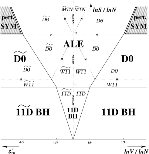
Figure 3.6: Phase diagram of the $D6$ system. The label dictionary is as follows: $\overline{M}TN$,$\widehat{M}TN$: black Taub-NUT geometry; $D6$,$\widetilde{D6}$: black D6 geometry; $D0$,$\widetilde{D0}$: black D0 geometry; $W11$,$\widetilde{W11}$: black 11D wave geometry; $11DBH$,$\widetilde{11D}BH$: 11D Light-Cone black hole; $\overline{D0}$,$\widetilde{\overline{D0}}$: black smeared D0 geometry; $\overline{W11}$,$\widetilde{\overline{W11}}$: black smeared 11D wave geometry; $\overline{11D}BH$,$\widetilde{\overline{11D}}BH$: 11D smeared Light-Cone black hole.

The $D6$ phase diagram has two important features (see Figure 3.6). First of all, the Maldacena limit keeps fixed the Planck scale ${\tilde{{\it l}}_{{\rm pl}}}\sim\frac{{\it l}_{{\rm pl}}^{2}}{R_{11}}V^{-2}$ of the high-entropy black Taub-NUT geometry [14]. Thus, gravity does not decouple, and the limit does not lead to a non-gravitational dual system that would serve as the definition of M-theory in such a spacetime. A symptom of this lack of decoupling of gravity is the negative specific heat $S\propto E^{3/2}$ of the high-entropy equation of state. This property is related to the breakdown of the usual UV-IR correspondence of Maldacena duality [68, 69]. The energy-radius relation of [69] determined by an analysis of the scalar wave equation in the relevant supergravity background, is in fact the relation between the horizon radius and the Hawking temperature of the associated black geometry; thus, for $p=6$ decreasing energy of the Hawking quanta is correlated to increasing radius of the horizon, as a consequence of the negative specific heat. This is to be contrasted with the situation for $p<5$, where the positive specific heat means increasing horizon radius correlates to increasing temperature; and $p=5$, where the Hawking temperature is independent of the horizon radius in the high-entropy regime. Now, temperature in any dual description must be the same as in the supergravity description. For $p<5$, the dual is a field theory; high temperature means UV physics dominates the typical interactions, leading to the UV-IR correspondence. For $p=5$, the dual is a little string theory; the temperature is unrelated to the horizon radius (and thus the total energy) on the gravity side, and unrelated to short-distance physics in the dual little string theory (since high-energy collisions of strings do not probe short distances). Hence the UV-IR correspondence already breaks down at this point. For $p=6$, there is nothing to say – large radius (large total energy) corresponds to low temperature of probes (Hawking quanta); and any dual description could not have high energy/temperature related to short distance physics, since it is a theory that contains gravity (so high energy makes big black holes).

A second key feature is the duality symmetry (c.f. [70]) $V\rightarrow V^{-1}$ of the diagram relating the $V<1$ structure to that discussed above for $V>1$. Note that this duality symmetry inverts the $T^{6}$ volume as measured in Planck units rather than string units. The duality interchanges momentum modes with fivebrane wrapping modes, while leaving membrane wrapping modes fixed; in other words, the dual space is that seen by the $M5$ brane.

3.3.2 The D1D5 system

As a further example of our methods, we have examined the D1D5 system on $T^{4}\times S^{1}$, which as we mentioned above can be considered as the little string theory of $Q_{5}$ fivebranes, with $Q_{1}$ units of string winding along the $S^{1}$.

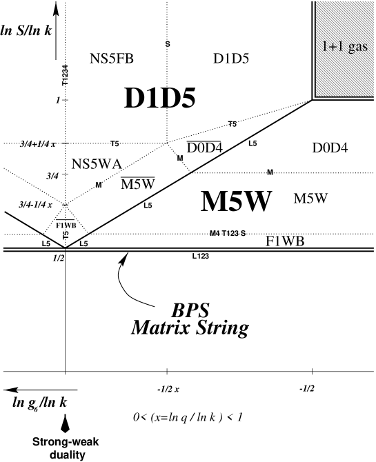
Figure 3.7: Thermodynamic phase diagram of little strings wound on the $S^{1}$ of $T^{4}\times S^{1}$, with $Q_{1}$ units of winding and $Q_{5}$ five branes. $k\equiv Q_{1}Q_{5}$ and $1<q\equiv Q_{1}/Q_{5}<k$. $g_{6}$ is the six dimensional string coupling of the $D1D5$ phase. The label dictionary is as follows: $D1D5$: black $D1D5$ geometry; $NS5FB$: black NS5 geometry with fundamental strings in IIB theory; $D0D4$: black D0D4 geometry; $\overline{D0D4}$: black smeared D0D4 geometry; $M5W$: black boosted M5 brane geometry; $\overline{M5W}$: black smeared boosted M5 brane geometry; $NS5WA$: black boosted NS5 branes in IIA theory; $F1WB$: black boosted fundamental strings in IIB theory; $\overline{F1WB}$: black smeared and boosted fundamental strings in IIB theory; L: localization transitions.

Figure 3.7 shows the thermodynamic phase diagram. In the Maldacena limit, this theory is a representation of the algebra of ${\cal N}=(4,4)$ superconformal transformations in 1+1d [10, 72, 73, 54, 55, 56]. We have defined $k\equiv Q_{1}Q_{5}$ and $q\equiv Q_{1}/Q_{5}$. We keep $k$ fixed, but $q$ may be viewed as a variable ranging between $1<q<k$, thus moving some of the dotted curves of duality transformation, but not altering phase transition curves. For $q\sim 1$, we can exchange the roles of $Q_{1}$ and $Q_{5}$ via duality transformations across the diagram; the structure is unchanged. The other limit, $q=k$, is the $Q_{5}=1$ bound. The vertical axis on the diagram is again the entropy, while the horizontal axis is the six-dimensional string coupling $g_{6}\equiv g_{s}/\sqrt{v}$ of the $D1D5$ patch, where $v=V_{4}/{\alpha^{\prime}}^{2}$ is the volume of the $T^{4}$ in string units (equivalently $g_{6}^{-2}$ is the volume of the $T^{4}$ in appropriate string units of the NS5FB phase). The phase diagram has a symmetry $g_{6}\rightarrow 1/g_{6}$ (inversion of the torus in the NS5FB phase); this is the T-duality symmetry of the little string theory. From the perspective of the $D1D5$ patch, we can consider the entire phase diagram as that of the 1+1d conformal theory that arises in the IR of this gauge theory, which is conjectured to be dual to the near-horizon geometry $AdS_{3}\times S^{3}\times T^{4}$ of the $D1D5$ system. In this patch, the D strings are wrapped on a cycle of size $R_{5}$. This parameter is absent from the scaling relations of all curves because of conformal symmetry. Analogous to the singly-charged brane systems we have been discussing, at high entropies there is a ‘1+1d gas’ phase at small $g_{6}$ (large effective $V_{4}$), which passes across a correspondence curve to the black brane phase as the coupling increases. Being determined by conformal symmetry and quantization of the central charge, the equation of state does not change across this ‘phase transition’. Starting in the ‘1+1d gas’ phase and decreasing the entropy, $S\sim k$ corresponds to the point where the thermal wavelength in the 1+1d conformal theory becomes of order the size of the box $R_{5}$. This is again a Horowitz-Polchinski correspondence curve from the side of lower entropies, analogous to the SYM theories at $S\sim N^{2}$ . There is a localization transition on the $R_{5}$ cycle cutting obliquely across the diagram. The localized phase can be interpreted as that of $M5$ branes with a large boost, thus connecting with the proposal of [57] for a Matrix theory of this system. The lower boundary of this phase occurs at entropies of order $S\sim\sqrt{k}$, where a BPS Matrix string phase emerges and the diagram is truncated at finite entropy. We find agreement with Vafa’s argument [74] that the BPS spectrum in the R sector of the D1D5 system is that of fundamental IIB strings carrying winding and momentum (sometimes called Dabholkar-Harvey states [75]). Similarly, chasing through the sequence of dualities for the D1D5 system on $K3\times S^{1}$, one finds the BPS spectrum consists of Dabholkar-Harvey states of the heterotic string.

For simplicity, we have restricted the set of parameters we have considered in the phase diagram to the entropy and the coupling $g_{6}$. It is straightforward to see what will happen as other moduli of the near-horizon geometry are varied. Consider for instance decreasing one of the $T^{4}$ radii keeping the total volume fixed. At some point, the appropriate low energy description will require T-duality on this circle, shifting from $D1$-branes dissolved into $D5$-branes, to $D2$-branes ending on $D4$-branes. One can then chase this duality around the diagram: The $NS5FB$ phase becomes $M2$-branes ending on $M5$-branes; the $NS5WA$, $\overline{D0D4}$, and $D0D4$ phases become $D1$-branes ending on $D3$-branes; and the $\overline{M5W}$ and $M5W$ phases become those of fundamental strings ending on $D3$ branes. The near-extremal $F1WB$ phase is unaffected. One can also imagine replacing the $T^{4}$ by K3. Moving around the K3 moduli space, when a two-cycle becomes small, a $D3$-brane wrapping the vanishing cycle becomes light; one should consider making a duality transformation that turns $Q_{1}$ or $Q_{5}$ into the wrapping number on this cycle.

Thus the D1D5 system appears to have a remarkably varied life. On the one hand, it can describe low-energy supergravity on a 6d space, namely $AdS_{3}\times S^{3}$; the common coordinate of the branes is the angle coordinate on $AdS_{3}$. This space parametrizes physics of the Coulomb branch of the gauge theory. On the other hand, the same system describes the ‘decoupled’ dynamics of the five-brane, another 6d system – except that the spatial coordinates are now $T^{4}\times S^{1}$, with the $T^{4}$ apparently related to the physics of the Higgs branch of the gauge theory, and the $S^{1}$ the dimension common to the branes. In the Maldacena limit, the theory is a representation of the 1+1d superconformal group.

Chapter 4 Black hole formation from Super Yang-Mills

4.1 Summary

A characteristic of the SYM phase diagrams we encountered in the previous chapters was the emergence, at strong Yang-Mills coupling and low entropies, of a Light-Cone black hole phase. We also encountered in the analysis for the phase diagram for the D1 system a phase describing a highly excited Matrix string. Both Matrix black hole and Matrix string have explicit realizations as excitations in the SYM fields as discussed in Sections 2.2 and 2.3. It would then be interesting to study the microscopic dynamics of the formation of the Light-Cone black hole phase as the string coupling of the Matrix string is tuned up. Previous analysis [76] of the collapse of a gravitationally interacting string into a black hole has yielded the conclusion that such a collapse accurs at weak string coupling provided that the system is compactified to low enough dimensions. This is because gravitational forces fall Coulombically as a power of the distance between the interacting objects and this power is smaller when the system is embedded in lower dimensions. Hence, the gravitational forces become stronger when we compactify to lower dimensions. The purpose of this chapter is to arrange a setting in the SYM theory where a Matrix string-Matrix black hole transition occurs readily; we then try to analyze the statistical mechanics of the formation of the black hole from SYM physics.

We would like $1+1$d SYM dynamics and a space-time compactified to low enough dimensions. We can achieve this dynamical setting by considering $p+1$d SYM theory compactified on a skewed torus $T^{p}$; i.e. $p-1$ radii of this torus will be accorded a different size from the $p$th radius. We consider Light-Cone M theory compactified on this torus, and we descend from it along the $p$th torus cycle to Light-Cone IIA theory; this cycle then gives us the string coupling $g_{\it str}$. The longitudinal boost direction is accorded radius size $R_{+}$. The remaining $p-1$ cycles fo the torus are tuned to the string scale. Our SYM theory then describes DLCQ IIA theory parametrized by $g_{\it str}$, ${\it l}_{{{\it str}}}$, $N$ and $R_{+}$. We pick an object in this IIA theory, a black hole or a highly excited string, and trace its history on a thermodynamic phase diagram.

Figure 4.1 is the phase diagram for the system of interest. We choose to work on a two dimensional cross section in the entropy-string coupling $S$-$g_{s}$ plane, with fixed longitundinal momentum $N\gg 1$. In principle, one is to take the thermodynamic limit $N\rightarrow\infty$ with $N/S$ fixed, to see criticality; transition between phases at finite but large $N$ are smooth crossovers. It is expected that, in the infinite $N$ limit, the physics tends to the appropriate critical behavior.

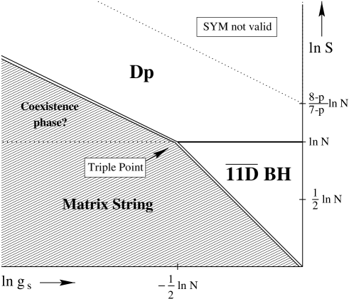
Figure 4.1: The proposed thermodynamic phase diagram for the $p+1$d SYM on the skewed torus for $p=4,5$. Equivalently, this is the phase diagram for DLCQ IIA theory on $T^{p-1}$. On the horizontal axis is the IIA string coupling, which is the aspect ratio of the SYM torus. The vertical axis is entropy.

The figure is a correct representation of physics for compactifications on $T^{4}$ or $T^{5}$, i.e. for $p=4,5$; these are the scenarios where the transverse non-compact space is small enough in dimensions for a black to form, while the torus is of low enough in dimensions for gravity to decouple from the SYM theory. The limit of validity of the SYM description for the DLCQ string theory is determined by the upper right curve. Above this line, the physics is not accurately described by super Yang-Mills theory; rather, one must pass to the six-dimensional little string theory as was done in the previous chapter. We will see that the dynamics of interest to us occurs outside this region. We identify several phases in this setting; a smeared black hole phase ($\overline{10D}$ BH), a Matrix string phase, a phase of $p+1$ dimensional strongly interacting SYM (i.e. the phase described by black Dp branes), and perhaps a ‘coexistence phase’ of a Matrix string with SYM vapor. There is a ‘triple point’, a thermodynamic critical point of the DLCQ string theory where three transition manifolds coincide.

A brief description of the physics of the diagram is as follows: In type IIA DLCQ string theory on $T^{p-1}$, with $p=4,5$, there exists a (longitudinally wrapped) D$p$-brane phase; it is unstable at $S\sim N$ to the formation of a black hole because of longitudinal localization effects. Along another critical curve (the diagonal line above $S\sim N$), the D$p$ brane freezes its strongly coupled excitations onto a single direction of the torus, making a transition to a perturbative string through the Horowitz-Polchinski correspondence principle. In this regime, the thermodynamics is that of a near-extremal fundamental (IIB) string supergravity solution, with curvature at the horizon becoming of order the string scale. The correspondence mechanism also applies on the other side of the $S\sim N$ transition; in this case, a Matrix black hole makes a transition to a Matrix string when it acquires string scale curvature at the horizon. A coexistence phase, where both Matrix string and SYM gas excitations contribute strongly to the thermodynamics, may exist in the region indicated on the diagram; this depends on the extent to which the object persists long enough to treat it using the methods of equilibrium thermodynamics.

Our second set of results concerns the dynamics that leads to the correspondence transitions, and is summarized by Figure 4.2. The plot depicts the mutual gravitational interaction energy between a pair of points on a typical (thermally excited) macroscopic Matrix string, as a function of the world-sheet distance $x$ along the string separating the two points.

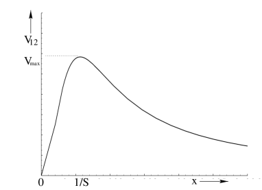
Figure 4.2: The string self-interaction potential as a function of relative separation $x$ along the string, for $p=4,5$.

This potential governs the dynamics of the Matrix string near a black hole or black brane transition, as it is approached from the weak string coupling side. A bump in the potential occurs at the thermal wavelength $N/S$ for $p=4,5$ (five or four noncompact spatial directions); in these dimensions, the correspondence transition to a black hole is indeed caused by the string’s self-interaction, as discussed in [76]. For smaller $p$ (more noncompact spatial directions), there is no bump; similarly, in [76] the self-interactions could not cause a spontaneous collapse to a black object. We will see that the height of the bump is proportional to the gravitational coupling, such that it ‘confines’ excitations of the string on the strong-coupling side of the correspondence transition.

This result supports the suggestion [34] to describe the black hole phase as clustered Matrix SYM excitations of size $N/S$. These correlated clusters were invoked in order that the object with $N>S$ can be localized in the longitudinal direction. Such a localization necessarily involves the longitudinal momentum physics of Matrix theory. We find that a plausible argument for the dynamics with this potential gives the two correspondence curves as the boundaries of validity of the Matrix string phase: for $N<S$, one finds the transition to the Dp brane phase shown in Figure (4.1); while for $N>S$, one finds the transition to the Matrix black hole phase. Accounting for the latter transition requires taking into consideration longitudinal momentum transfer effects as in [34]; we justify this by a string theory amplitude calculation involving winding number exchange in a dual picture given in Appendix F. We thus conclude that we have identified the characteristics of the microscopic mechanism of black hole formation from the SYM point of view.

In the next section, we map the phase diagram in the region of the thermodynamic parameter space of interest to us. In Section 4.3, we analyze the statistical mechanics of the SYM theory near the triple point.

4.2 The phase structure

4.2.1 Preliminaries

A DLCQ IIA theory descends from the DLCQ $M$ theory described above; we choose string scale compactification

$$R_{i}\sim{\it l}_{{{\it str}}}\ \ \ \mbox{for }i=1\ldots p-1\ ,$$ (4.1)

with

$$R_{p}=g_{s}{\it l}_{{{\it str}}}\ \ \ {\it l}_{{\rm pl}}^{3}=g_{s}{\it l}_{{{\it str}}}^{3}\ ,$$ (4.2)

and a perturbative IIA regime

$$g_{s}\ll 1\ .$$ (4.3)

We can in principle relax (4.1) at the expense of introducing new state variables, and a more complicated (and richer) phase diagram; for simplicity, we will stick to this ‘IIA regime’. We write the dictionary between our IIA theory and the Matrix SYM

$$g_{Y}^{2} = ~{}(2\pi)^{p-2}(ag_{s})^{p-3}\ ,$$

$$\Sigma_{i} = ~{}g_{s}a\ \ \ \mbox{for }i=1\ldots p-1\ ,$$

$$\Sigma_{p} = ~{}a\ ,$$ (4.4)

$$V \equiv ~{}\Sigma_{i}^{p-1}\Sigma_{p}=g_{s}^{p-1}a^{p}\ ,$$

with

$$a\equiv\frac{{\alpha^{\prime}}}{R_{+}}\ .$$ (4.5)

We chose (4.3) so that we have $\Sigma_{i}\ll\Sigma_{p}$, simplifying our analysis later. Note that $V$ here stands for the volume of the SYM torus.

We study finite temperature physics of this IIA theory with the finite temperature vacuum of the corresponding SYM.

4.2.2 The phase diagram

Given that we are working with Matrix theory on $T^{4}$ and $T^{5}$, the first question that must be addressed concerns the validity of the description, given that SYM 4+1d and 5+1d are non-renormalizable. New degrees of freedom are required to make sense of the SYM dynamics as we probe it in the UV, i.e. as we navigate outward in the corresponding supergravity solution. These new degrees of freedom for SYM 4+1d and 5+1d are associated with the onset of strong coupling dynamics; the validity of the theories at different energy scales is then determined by looking at the size of the dilaton vev at different locations in the supergravity solution. For finite temperatures, physics at the thermal wavelength of the SYM is identified with physics at the horizon of the near extremal solution (1.9). The finite temperature vacuum of the $4+1$d and $5+1$d SYM is a valid thermodynamic description of the DLCQ IIA theory when

$$\left.e^{\phi}\right|_{r_{o}}\ll 1\Rightarrow S\ll N^{\frac{8-p}{7-p}}g_{s}^{-1}\ .$$ (4.6)

This is a purely geometric statement, in terms of the horizon area and string coupling. For entropies satisfying this bound, the SYM statistical mechanics obeys the equation of state

$$\left(aE\right)^{p-9}\sim\left(\frac{S^{2}}{N}\right)^{p-7}g_{\it str}^{4}\ .$$ (4.7)

From our discussion in the earlier chapters, we know that this phase will localize into a black hole for $S<N$. This is a $11$D Schwarzchild hole smeared over $T^{p}$; it appears as a black hole living in DLCQ IIA theory smeared on $T^{p-1}$. Its equation of state is

$$E^{p-9}_{bh}\sim E_{int}^{p-9}\left(\frac{N}{S}\right)^{2}\ .$$ (4.8)

The Schwarzschild black hole geometry will become stringy when its curvature near the horizon becomes of the order of the string scale; the emerging state is a Matrix string in the Matrix conjecture language, i.e. a $1+1$d dynamics with $Z_{N}$ holonomy on $\Sigma_{p}$. Minimizing the Gibbs energy between the Matrix string

$$E\sim a^{-1}\frac{S^{2}}{N}$$ (4.9)

and the Matrix black hole phases leads to the Horowitz-Polchinski correspondence curve [41, 76]

$$S\sim g_{s}^{-2}\ .$$ (4.10)

This is a statement independent of $N$ and $p$. At $g_{c}\sim N^{-1/2}\sim N_{\rm\scriptscriptstyle osc}^{-1/4}$, where $N_{\rm\scriptscriptstyle osc}$ is the string oscillator level, there exists an interesting critical point.

We next deal with finite size effects in the Dp brane phase which are due to the other radii $\Sigma_{i}$. Because the torus is skewed, the thermal wavelength probes a $p-1$ dimensional torus. We expect a localization transition to a phase consisting of the geometry of D1 branes. Equating the energies of (4.7) for $p=1$ and for general $p$, we get the transition point

$$S\sim\sqrt{N}g_{s}^{-1}\ .$$ (4.11)

We find however that, near this transition point, the D1 vacuum is strongly coupled at the horizon; the S-dual geometry is that of black fundamental strings in IIB theory. No change of equation of state occurs through this duality transformation. The curvature at the horizon of the black IIB string solution is found to become of order the string scale at precisely (4.11), beyond which a Matrix string description emerges. Our analysis leading to (4.11) is then valid. We can further check the correctness of this conclusion by matching the equation of state (4.7) with that of the Matrix string (4.9), the latter being the dominant phase on the other side of this correspondence curve. The result is again (4.11). We conclude that the Dp brane phase makes a transition to a Matrix String at (4.11).

Finally, we note that we assumed above that there exists a well defined Matrix string description for $N<S$. In this regime, the thermal wavelength on the Matrix string is smaller than the UV cutoff imposed by the discretized nature of the matrices. Our procedure may be equivalent to an analytical continuation of the Matrix string phase into a regime where the description may not be fully justified; this is in the same spirit as the extension of the Van der Waals equation of state into the gas-liquid coexistence region, which one uses to identify the emergence of the liquid phase[77]. Furthermore, the regime $N<S$ is similar to the Hagedorn regime [78, 79], in that the temperature remains constant as the system absorbs heat. We speculate that the $N<S$ regime of the Matrix string near the triple point is characterized by a coexistent phase of a string with SYM vapor.

As a unifying probe for all the transitions, we observe that the ‘mass per unit charge’ $q$ defined by

$$q\equiv\frac{M}{N}$$ (4.12)

scales on the various transition curves as

Matrix String-Dp brane transition	$\rightarrow$	$q^{-1}\sim h_{\rm eff}{\it l}_{{{\it str}}}$
Matrix String-Coexistence Phase Transition	$\rightarrow$	$q^{-1}\sim{\it l}_{{{\it str}}}$
Matrix String-Black Hole Transition	$\rightarrow$	$q^{-1}\sim h_{\rm eff}^{2}{\it l}_{{{\it str}}}$
Black Hole-Dp brane transition	$\rightarrow$	$q^{-1}\sim h_{\rm eff}^{2/(9-p)}{\it l}_{{{\it str}}}$

with the effective coupling

$$h_{\rm eff}^{2}\equiv g_{s}^{2}N\ .$$ (4.13)

From the point of view of the DLCQ string theory characterized by the parameters $g_{s}$, ${\it l}_{{{\it str}}}$ and $N$, this scaling on the transition curves is a non-trivial signature of a unifying framework underlying the physics of criticality of the theory. Note also that the $g_{s}^{2}N$ combination is not the ’t Hooft coupling of the SYM description; recall that $g_{s}$ is a modulus of the torus compactification. From the point of view of field theory, the various transitions that we have identified are predictions about the thermodynamics of 4+1d, 5+1d SYM on the torus well into non-perturbative field theory regimes.

4.3 The interacting Matrix string

In this section, we study the dynamics near the triple point in greater detail from the side of the Matrix string. In Section 2.2, it was argued that the Matrix black hole phase, as a configuration of the SYM fields, can be thought of as a gas of $S$ distinguishable clusters of D0 branes, each cluster consisting of $N/S$ partons. The system is self-interacting through the $v^{4}/r^{7}$ interaction, or its smeared form on the torus. This phase of clustered D0 branes may be an effective description, i.e. thermodynamically strongly correlated regions of a metastable state; or more optimistically, it might be a microscopic description associated with formation of bound states like in BCS theory. We will try here to investigate the Matrix string dynamics so as to reveal the signature of the clusters as we approach the correspondence curve. The aim is to identify a possible dynamical mechanism for black hole formation, and determine the correspondence curve from such a microscopic consideration.

In Section 4.3.1, we derive the potential between two points on the Matrix string; in view of the Matrix conjecture, we can do this by expanding the Dirac-Born-Infeld (DBI) action of a D-string in the background of a D-string. We then evaluate the expectation value of this potential in the free string ensemble at fixed temperature. In Sections 4.3.2 and 4.3.3, we analyze the characteristic features of the potential, particularly noting the bump for $p=4,5$ that we alluded to in the Introduction. In Section 4.3.4, we comment on the dynamics implied by the potential, particularly in regard to the phase diagram derived earlier.

4.3.1 The potential

In this section, we derive the potential between two points on the Matrix string by expanding the DBI action for a D-string probe in the background geometry of a D-string. We then check the validity of the DBI expansion, and evaluate the expectation value of the potential in the thermal ensemble of highly excited Matrix strings. The details of the finite temperature field theory calculations are collected in Appendix E.

A IIA string in Matrix string theory is constructed in a sector of field configurations described by diagonal matrices, with a holonomy in $Z_{N}$; a nonlocal gauge transformation converts this into ’t Hooft-like twisted boundary conditions on the transverse excitations of the eigenvalues of the matrices, as described in detail in [36, 62, 80, 35]. The conclusion is that the eigenvalues are sewn together into a long string, and a IIA string emerges as an object looking much like a coil or ‘slinky’ wrapped on $\Sigma_{p}$. The self-interactions of this string are described by integrating out off-diagonal modes between the well-separated strands. Alternatively, making use of the Matrix conjecture, this effective action can be obtained from supergavity, by expanding the Born-Infeld action of a D-string in the background of a D-string . We will follow this prescription to calculate the gravitational self-interaction potential between two points on a highly excited Matrix string.

The Born-Infeld action for N D-strings is given by [24]

$$S=-\frac{1}{2\bar{\alpha}^{\prime}\bar{g}_{s}}\left[\int d^{2}\sigma e^{-\phi}\mbox{Tr}\mbox{Det}^{1/2}\left(G_{ab}+B_{ab}+2\pi{\alpha^{\prime}}F_{ab}\right)-N\int C_{RR}^{(2)}\right],$$ (4.14)

where we have assumed commuting matrices so that there is no ambiguity in matrix orderings in the expansion, and $\bar{g}_{s}$ is the dilaton vev at infinity. We choose $\sigma^{1}$ to have radius $\Sigma_{p}$, turn off gauge and NS-NS fluxes,

$$B_{ab}=F_{ab}=0\ ,$$ (4.15)

and choose the static gauge

$$X^{0} = ~{}\sigma^{0}\mbox{1}\ ,$$ (4.16)

$$X^{1} = ~{}\sigma^{1}\mbox{1}\ .$$

A single D-string background in the string frame is given by [81]

$$ds_{10}^{2} = ~{}h^{-1/2}(-dt^{2}+dx^{2})+h^{1/2}(d\vec{x})^{2}$$

$$\vskip 6.0pt plus 2.0pt minus 2.0pte^{\phi} = ~{}h^{1/2}\hfill$$ (4.17)

$$C_{01} = ~{}h^{-1}\hfill$$

$$h = ~{}\left(\frac{r_{0}}{r}\right)^{7-p}\ ,$$

(recall $p$ is the torus dimension) and we define $D\equiv 7-p$. The string is taken to have no polarizations on the torus, nor any Kaluza-Klein charges. Here, we have followed the prescription in [82, 83], where we T-dualized the D-string solution to a D0 brane, lifted to 11 dimensions, compactified on a lightlike direction, and T-dualized the solution to the one above. The only change is in replacing $1+(r_{0}/r)^{7-p}\rightarrow(r_{0}/r)^{7-p}$. By Gauss’ law,

$$r_{0}^{D} = ~{}c_{D}\frac{g_{s}^{2}}{R_{+}^{2}}{\it l}_{{{\it str}}}^{9-p}\ ,$$ (4.18)

$$c_{D} \equiv ~{}\frac{(2\pi)^{7}}{2\pi^{D/2}}\Gamma(D/2)\ ,$$

where we have made use of the needed dualities to express things in our IIA description. Putting in the background, we have

$$S = ~{}-\frac{1}{{\alpha^{\prime}}}\int^{\Sigma_{p}N}\ h^{-1}\left(1+hK+h^{2}V\right)^{1/2}-h^{-1}$$ (4.19)

$$K \equiv ~{}{X^{\prime}}^{2}-{\dot{X}}^{2}=4\partial_{+}X.\partial_{-}X$$

$$\vskip 6.0pt plus 2.0pt minus 2.0ptV \equiv ~{}4((\partial_{+}X.\partial_{-}X)^{2}-(\partial_{+}X)^{2}(\partial_{-}X)^{2})\ .$$

We note that, as the limit of the action indicates, we have made use of the $Z_{N}$ holonomy that sews the rings of the slinky together. Expanding the square root yields the Hamiltonian

$$H = \int^{\Sigma_{p}N}\frac{1}{2{\alpha^{\prime}}}({\dot{X}}^{2}+{X^{\prime}}^{2})+c_{D}^{\prime}\frac{g_{s}^{2}{\it l}_{{{\it str}}}^{7-p}}{R_{+}^{2}r^{7-p}}\times$$ (4.20)

$$\left\{(\partial_{+}X)^{2}(\partial_{-}X)^{2}-\left[(\partial_{+}X)^{2}+(\partial_{-}X)^{2}\right](\partial_{+}X.\partial_{-}X)\right\}\ .$$

Let us check the validity of the DBI expansion we have performed. We would like to study dynamics of the string squeezed at most up to the string scale, the correspondence point; setting $r\sim{\it l}_{{{\it str}}}$ in $h$, we get

$$h\sim\left(\frac{g_{s}{\it l}_{{{\it str}}}}{R_{+}}\right)^{2}\ .$$ (4.21)

From elementary string dynamics, we have

$$\langle K\rangle\sim\left(\frac{R_{+}S}{{\it l}_{{{\it str}}}N}\right)^{2}\ ,$$ (4.22)

where brackets indicate thermal averaging at fixed entropy $S$. It can be shown from the results of the next section that

$$\langle V\rangle_{max}\sim\langle K\rangle^{2}\ ,$$ (4.23)

and that $\langle V\rangle$ will have a definite maximum for all $p$. We now see from (4.19), (4.21), (4.22), and (4.23), that our DBI expansion is a perturbative expansion in

$$\varepsilon=g_{s}\frac{S}{N}\ .$$ (4.24)

We then need

$$S\ll Ng_{s}^{-1}\ .$$ (4.25)

A glance at Figure 4.1 reveals that we are well within the region of interest.

The potential in this expression is the interaction energy between a D-string probe and a D-string source. Using the residual Galilean symmetry in the DLCQ, and assuming string thermal wavelengths $>\Sigma_{p}$ (the ‘slinky regime’), we deduce that the potential between two points on the Matrix strings denoted by the labels $1$ and $2$ is

$$V_{12}={K}_{D}\frac{g_{s}^{2}{\it l}_{{{\it str}}}^{5-p}}{R_{+}}\frac{\left\{(\partial_{+}X_{r})^{2}(\partial_{-}X_{r})^{2}-\left[(\partial_{+}X_{r})^{2}+(\partial_{-}X_{r})^{2}\right](\partial_{+}X_{r}.\partial_{-}X_{r})\right\}}{\left(X_{r}^{2}\right)^{D/2}}\ ,$$ (4.26)

where

$$X_{r}\equiv X_{2}-X_{1}.$$ (4.27)

and $K_{D}$ is a horrific numerical coefficient we are not interested in.

Ideally, one should self-consistently determine the shape distribution of the string in the presence of this self-interaction; however, this is rather too complicated to actually carry out. To first order in small $g_{s}$, the effect of the potential is to weigh different regions of the energy shell in phase space [84] by a factor derived from its expectation value in the free string ensemble. We will discuss the dynamics in the presence of the potential in somewhat more detail below. For now, in light of this weak-coupling approximation scheme, we would like to calculate the expectation value of the potential in a thermodynamic ensemble consisting of a highly excited free string with fixed entropy $S$. From the Matrix string theory point of view, this is essentially a problem in finite temperature field theory, where we will deal with a two dimensional Bose gas (ignoring supersymmetry; the fermion contribution is similar) on a torus with sides $\Sigma_{p}N$ and $\beta=1/T$, $\beta$ being the period of the Euclidean time. Using Wick contractions, we can then express the potential in terms of the free Green’s functions; we defer the details to Appendix E. We get

$$V_{12}=\alpha_{D}g_{s}^{2}\frac{{\it l}_{{{\it str}}}^{5-p}}{R_{+}}\frac{K^{zz}_{12}K^{\bar{z}\bar{z}}_{12}}{\left(-K_{12}\right)^{D/2}},$$ (4.28)

where $\alpha_{D}$ is a dimension dependent numerical coefficient,

$$K_{12}\equiv K_{\Delta}\equiv-{\alpha^{\prime}}\left<X_{1}X_{2}\right>\equiv-{\alpha^{\prime}}G_{12}\ ,$$ (4.29)

is the Green’s function of the two dimensional Laplacian on the torus, and $K^{zz}_{12}$ is its double derivative with respect to the $z$ complex coordinate of the Riemann surface representing the Euclideanized world-sheet.

4.3.2 The thermal free string

The thermodynamic properties of the Matrix string at inverse temperature $\beta$ are determined by the Green’s function of the Laplacian on the worldsheet torus of sides $(\Sigma,\beta)$, where $\Sigma\equiv\Sigma_{p}N$. It is known from CFT on the torus that this is given by[85, 86]

$$G_{12}=-\frac{1}{2\pi}\ln\left|\frac{\theta_{1}\left(\frac{z}{\Sigma}|\tau\right)}{\theta^{\prime}_{1}\left(0|\tau\right)}\right|+\frac{1}{2\tau_{2}}\left(\mbox{Im}\frac{z}{\Sigma}\right)^{2},$$ (4.30)

where

$$\tau\equiv i\frac{\beta}{\Sigma}\equiv i\tau_{2}=\frac{i}{S}.$$ (4.31)

Here $\beta$ can be obtained from free string thermodynamics. All correlators and their derivatives must eventually be evaluated on a time slice corresponding to the real axis in the $z$ plane.

Divergences will be seen in correlators due to infinite zero point energies. The conventional approach is to introduce a normal ordering scheme giving the vacuum zero expectation value in such situations, i.e. throwing away disconnected vacuum bubbles. In our case, the string has a classical background due to its thermal excitation. To renormalize finite $T$ correlators, we subtract the zero temperature limit from each propagator. This corresponds to

$$\mbox{$\langle{f(X)}\rangle$}\sim f({\textstyle{\delta\over\delta J}})\ln Z_{T}[J]\rightarrow f({\textstyle{\delta\over\delta J}})\ln Z_{T}[J]-f({\textstyle{\delta\over\delta J}})\ln Z_{T=0}[J]=f({\textstyle{\delta\over\delta J}})\ln\Bigl{(}\frac{Z_{T}[J]}{Z_{T=0}[J]}\Bigr{)}.$$ (4.32)

From the expression for $Z[J]$, we see that this amounts to correcting the Green’s functions as

$$K\rightarrow K_{T}-K_{T=0}.$$ (4.33)

This subtraction removes the divergent zero-point fluctuations of nearby points on the string, while leaving the effects due to thermal fluctuations.

Defining

$$x\equiv\frac{z}{\Sigma}\ ,$$ (4.34)

we then have, subtracting the zero temperature part,

$$K_{\Delta}\rightarrow{\alpha^{\prime}}\left(\frac{1}{4\pi}\ln g\bar{g}+\frac{1}{8\tau_{2}}\left(x-\bar{x}\right)^{2}\right),$$ (4.35)

with

$$\ln g=\sum_{n=1}\ln\left(\frac{1-2q^{n}\cos(2\pi x)+q^{2n}}{\left(1-q^{n}\right)^{2}}\right).$$ (4.36)

We can now make use of $\tau_{2}\ll 1$ for $S\gg 1$, to write this sum as an integral

$$\ln g=\frac{1}{2\pi\tau_{2}}\int_{0}^{e^{-2\pi\tau_{2}}}\frac{dv}{v}\ \ \ln\left(\frac{1-2v\cos(2\pi x)+v^{2}}{\left(1-v\right)^{2}}\right).$$ (4.37)

This integral can be evaluated to yield

$$\ln g=\frac{1}{2\pi\tau_{2}}\left(2Li_{2}e^{-2\pi\tau_{2}}-Li_{2}e^{-2\pi\tau_{2}+2\pi xi}-Li_{2}e^{-2\pi\tau_{2}-2\pi xi}\right),$$ (4.38)

where $Li_{2}$ is the PolyLog function of base 2, related to the Lerch $\Phi$ function [87]. We then have

$$K_{\Delta}=\frac{{\alpha^{\prime}}}{2\pi}\ln g\ ,$$ (4.39)

with $x$ here being real, and representing the equal-time separation between two points on the string, $x=x_{1}-x_{2}$, as a fraction of the total length $\Sigma$ ($0<x<1$). The asymptotics are

$$K_{\Delta}\simeq\left[\begin{array}[]{cl}{\alpha^{\prime}}Sx&\mbox{ for }\tau_{2}\ll 1\\ \frac{{\alpha^{\prime}}}{\pi}S^{2}x^{2}&\mbox{ for }2\pi x\ll 1\end{array}\right.,$$ (4.40)

The first line is a well-known result of Mitchell and Turok [88] calculated originally using the microcanonical ensemble. It shows random walk scaling $\sqrt{\mbox{$\langle{R^{2}}\rangle$}}\sim N_{\rm\scriptscriptstyle osc}^{1/4}x^{1/2}$. The second line is new and valid for small separations on the string; it is the statement that within the thermal wavelength $\beta$ of the the excited string, the string is stretched, scaling as $\sqrt{\mbox{$\langle{R^{2}}\rangle$}}\sim N_{\rm\scriptscriptstyle osc}^{1/2}x$. This is intuitively expected, as regions on the string within the typical thermal wavelength will be strongly correlated in the thermodynamic sense. This change in the scaling is crucial to what we will soon see in the behavior of the potential between strands. $-K_{\Delta}$ is plotted in Figure 4.3.

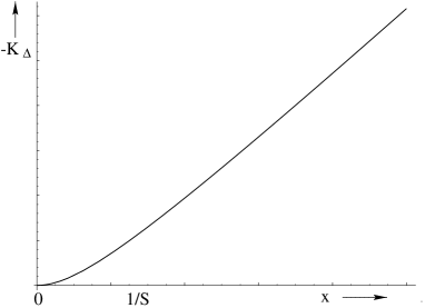
Figure 4.3: $-K_{\Delta}$ as a function of the string separation parameter $x$; we see the change of scaling from $x^{2}$ to $x$.

Next, consider the derivatives of the correlators, evaluated on the real axis. We have

$$\partial_{x}K_{\Delta}=\partial_{\bar{x}}K_{\Delta}=\frac{-i{\alpha^{\prime}}}{2(2\pi)^{2}\tau_{2}}\ln\left(\frac{1-e^{-2\pi\tau_{2}-2\pi ix}}{1-e^{-2\pi\tau_{2}+2\pi ix}}\right).$$ (4.41)

We also have

$$\partial_{x}\partial_{\bar{x}}K_{\Delta}=\frac{-{\alpha^{\prime}}}{4\tau_{2}},$$ (4.42)

or

$$K^{z\bar{z}}_{\Delta}\rightarrow 0,$$ (4.43)

since we subtract the zero temperature result. The most relevant term is

$$\partial_{x}^{2}K_{\Delta}=\partial_{\bar{x}}^{2}K_{\Delta}=-\frac{{\alpha^{\prime}}}{\tau_{2}}\frac{1-e^{2\pi\tau_{2}}\cos(2\pi x)}{e^{4\pi\tau_{2}}-2e^{2\pi\tau_{2}}\cos(2\pi x)+1}+\frac{{\alpha^{\prime}}}{4\tau_{2}},$$ (4.44)

or

$$\Sigma^{2}K^{zz}_{\Delta}=\Sigma^{2}K^{\bar{z}\bar{z}}_{\Delta}\rightarrow-\frac{{\alpha^{\prime}}}{\tau_{2}}\frac{1-e^{2\pi\tau_{2}}\cos(2\pi x)}{e^{4\pi\tau_{2}}-2e^{2\pi\tau_{2}}\cos(2\pi x)+1}-\frac{{\alpha^{\prime}}}{\tau_{2}}\frac{1}{e^{2\pi\tau_{2}}-1}$$ (4.45)

(again we subtract the zero temperature part).

This yields the asymptotics

$$(N\Sigma_{p})^{2}K^{zz}_{\Delta}\simeq\left[\begin{array}[]{cl}{\alpha^{\prime}}S^{2}+\frac{\pi}{12}(5+\cos(2\pi x))(\csc(\pi x))^{2}+O(\tau_{2}^{2})\rightarrow{\alpha^{\prime}}S^{2}&\mbox{ for }\tau_{2}\ll 1\\ {\alpha^{\prime}}S^{4}x^{2}&\mbox{ for }2\pi x\ll 1\end{array}\right..$$ (4.46)

$K^{zz}_{\Delta}$ is plotted in Figure 4.4 as a function of $x$.

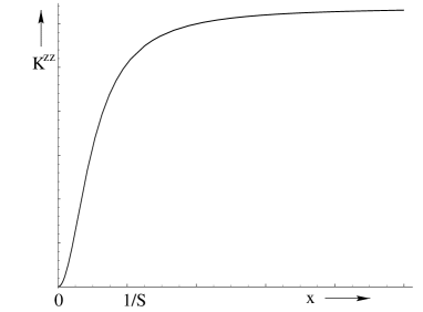
Figure 4.4: $K^{zz}_{\Delta}$ as a function of the string separation parameter $x$; we see the flattening of the correlation at large $x$. For small $x$, small relative stretching or motion is implied; for larger $x$, the flattening indicates a constant correlation in the relative stretching of the string.

4.3.3 The bump potential

We now put together equations (4.39) and (4.45) in the potential of (4.28) to get the asymptotics

$$V_{12}\simeq g_{s}^{2}\frac{R_{+}^{3}}{{\alpha^{\prime}}^{3}N^{4}}\left[\begin{array}[]{cl}S^{(8-D)/2}x^{-D/2}&\mbox{ for }\tau_{2}\ll 1\\ S^{8-D}x^{4-D}&\mbox{ for }2\pi x\ll 1\end{array}\right..$$ (4.47)

For $p>3$, $V_{12}\rightarrow 0$ as $x\rightarrow 0$; at larger $x$, it decays as $x^{-D/2}$. At the thermal wavelength $x\sim 1/S$, both expressions give

$$V_{max}\simeq g_{s}^{2}\frac{R_{+}^{3}}{{\alpha^{\prime}}^{3}N^{4}}S^{4}.$$ (4.48)

Note that in this expression the dimension dependence in the power of $S$ conspires to vanish. For $p=3$, $V_{12}\sim S^{4}$ for $x\rightarrow 0$, while for $p<3$, $V_{12}\rightarrow\infty$ for $x\rightarrow 0$; in both of these latter cases, the potential decays as $x^{-D/2}$ for larger $x$.

The conclusion can be summarized as follows. For $p=4$ and $p=5$, there exists a bump in the potential of height proportional to $S^{4}$ at the thermal wavelength on the string; for $p=3$, the bump smoothes to a flat configuration where the difference between the potential at the thermal wavelength separation and at $x=0$ is of order unity. Finally, for $p<3$, the bump disappears altogether and the potential blows up at the origin signaling the breakdown of the description. This potential is plotted in various cases in Figure 4.2 of the Introduction and Figure 4.5.

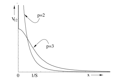
Figure 4.5: The potential as a function of $x$ for dimensions $p=3$ and $p=2$.

The presence or absence of the bump is a result of two competing effects: First of all, the increasingly singular short-distance behavior of the Coulomb potential (4.26) with increasing dimension $D$; and secondly, the strong correlation of neighboring points on the string, which makes $(\partial X_{1}-\partial X_{2})$ decrease as the separation along the string decreases (inside a thermal wavelength).

We observe that:

• The bump occurs at separations of $1/S$ of a fraction of the whole length of the string; in the Matrix theory language, this corresponds to a bump about matrices of size $N/S$.

• The presence or absence of the bump as a function of the number of non-compact space dimensions correlates with the observations of [76], given that in the DLCQ, the light-like direction reduces the number of non-compact dimensions by one. In [76], considering the gravitational self-interactions of a highly excited string, the authors demonstrated that the string collapses into a black hole at weak string coupling (4.10) provided that there are less than six non-compact space dimensions. Correspondingly, we observe the bump in the potential for the scenarios where we have four or five non-compact space dimensions in Light-Cone IIA theory.

• As described in [34], a Matrix black hole can be described by SYM excitations clustered within matrices of size $N/S$, the location of the bump. Furthermore, we will shortly reproduce, from scaling arguments regarding the dynamics of this potential, the two correspondence lines determined from thermodynamic considerations above.

We then conclude that we have identified the characteristic signature of black hole formation in the Matrix SYM.

4.3.4 Dynamical issues and black hole formation

The dynamics of this potential near a phase transition point is certainly complicated. Intuitively, we expect that as we approach a critical point, instabilities develop, an order parameter fluctuates violently, perhaps related to some measure of the $Z_{N}$ symmetry; it is reasonable to expect the characteristic feature of the potential, the confining bump, plays a crucial role in the dynamics of the emerging phase. Let us try to extract from these results the scaling of the correspondence curves.

First let us motivate the use of the expectation value of the potential in the free string ensemble. We indicated earlier that this quantity is qualitatively related to the effect of the interactions, assuming they are weak enough, on the energy shell in phase space covered by the free string. The partition function becomes, schematically

$$Z\sim\mbox{Tr }e^{H_{0}+V}\sim e^{\left<V\right>_{0}}\mbox{Tr }e^{H_{0}}\ ,$$ (4.49)

so that phase space is weighed by an additional factor related to the expectation value of the potential in the free ensemble $\left<V\right>_{0}$. This is also similar to the RG procedure applied to the 2d Ising model, where the context and interpretation is slightly different [84].

Using equation (4.28), the potential energy content of the Matrix string is given by

$$V\sim\int_{0}^{N\Sigma_{p}}d\sigma_{-}\ \left(S^{4}g_{s}^{2}\frac{R_{+}^{3}}{{\alpha^{\prime}}^{3}N^{4}}\right)\left(N\Sigma_{p}\right)v_{12}\ ,$$ (4.50)

where we have integrated over one of the two intergals of the translationally invariant two-body potential, and scaled $v_{12}$ such that its maximum is of order 1, independent of any state variables; however, the shape of $v_{12}$ still depends on $N$ and $S$. This expression represents the interaction energy between two points on the coiled Matrix string at fixed separation $\sigma_{-}$. From the point of view of Matrix theory physics, the string’s fundamental dynamical degrees of freedom are the windings on the coil; we expect a transition in the dynamics of the object when there is a competition between forces on an individual winding. In the present case, the two forces are nearest neighbor elastic interaction and the gravitational interaction. A single string winding being wrapped on $\Sigma_{p}$ worth of world-sheet, the maximum potential energy it feels can be read from equation (4.50)

$$v_{max}\sim S^{4}g_{s}^{2}\frac{R_{+}^{3}}{{\alpha^{\prime}}^{3}N^{4}}N\Sigma_{p}^{2}\ ,$$ (4.51)

and is due to its interaction with strands a thermal wavelength away. Its thermal energy caused by nearest neighbour interactions is read off equation (4.22)

$$\kappa\sim\frac{\left<K\right>}{{\alpha^{\prime}}}\Sigma_{p}\ .$$ (4.52)

The two forces compete when

$$S\sim\sqrt{N}g_{s}^{-1}\ .$$ (4.53)

At stronger coupling, the forces due to the gravitational interaction dominate those of the nearest neighbor stretching and decohere neighboring strands’ velocities. The free string evaluation of the interaction, equation (4.28), is no longer valid; one expects a phase transition to occur. Equation (4.53) is our matching result of (4.11) between the string and $p+1$d interacting SYM phase. Here, we are assuming an analytical continuation of the Matrix string phase to the region $N<S$ in the phase diagram; our suggestion that this region is associated with a coexistence phase is consistent with this procedure.

To account for the correspondence curve for $N>S$, we now recall that in the discussion of clustered D0 branes of [34], the virial treatment of the $v^{4}/r^{7}$ interaction had to be corrected by a factor in order to reproduce the black hole equation of state; the origin of this correction was argued to be interaction processes between the clusters involving the exchange of longitudinal momentum. Under the assumption that these effects are of the same order as zero momentum transfer processes, a correction factor of $N/S$ was applied. Using a chain of dualities, we can quantify the effect of longitudinal momentum transfer physics by studying the scattering amplitude in IIB string theory with winding number exchange. We do this in Appendix F, where we find that, for exchanges of windings up to order $N/S$, the winding exchange generates an interaction identical to that of zero longitudinal momentum exchange; for higher winding exchanges, the interactions are much weaker. These winding modes, represent the sections of the Matrix string within the thermal wavelength, $N/S$ worth of D-string windings. Thus we modify the $v_{12}$ potential above by the factor $N/S$, which accounts in the scaling analysis for the effect of longitudinal momentum transfer physics in the Matrix string self-interaction potential. Applying the virial theorem between equation (4.52) and $N/S$ times equation (4.51) yields the Matrix string-Matrix black hole correspondence point at

$$S\sim g_{s}^{-2}\ ,$$ (4.54)

as needed.

We can now interpret our results as follows. The bump potential accounts for the matching of the string phase onto both $N<S$ and $N>S$ phases, one involving partons interacting without longitudinal momentum exchange (the Matrix string-Dp brane curve in Figure 4.1), and the other being the Matrix black hole phase of parton clusters of size $N/S>1$ interacting in addition by exchange of longitudinal momentum (the Matrix string/Matrix black hole correspondence curve of Figure 4.1). In the latter case, the location of the confining bump correlates with matrices of size $N/S$. In the former case, the correlations are finer than the UV matrix cutoff; a better understanding of this latter issue obviously needs a more quantitative analysis of the $N<S$ Matrix string regime. This analysis further substantiates the identification of the bump potential as the signature of black hole formation from Matrix SYM, as well as justifying the new Matrix string-Dp brane transition microscopically.

Appendix A A few words about black holes

We review in this appendix some background material relevant to black hole physics. Black holes appear to obey the four laws of thermodynamics with the following identifications: the area of the horizon $A$ is mapped to the entropy $S$ of the black hole

$$S\sim\frac{A}{2\kappa_{D}^{2}}\ ,$$ (A.1)

where $D$ is the space-time dimension, and $2\kappa_{D}^{2}$ is the gravitational coupling; the temperature is given by the surface gravity ; and the mass is identified with the energy of the given thermodynamic state.

A geometry in general relativity is accorded a mass or energy by studying probe dynamics at large distances away from the source responsible for the curving of the space-time. This gives a measure for the energy content of the system as seen by an observer at infinity. For a metric of the form [89]

$$ds^{2}=-A(r)dt^{2}+B(r)dr^{2}+r^{2}C(r)d\Omega_{D-p-2}^{2}+D(r)dy^{i}\ dy^{i}\ ,$$ (A.3)

$i$ running over $p$ space coordinates, the mass per unit $p$ dimensional volume is given by

$$M = -\frac{\Omega_{D-p-2}}{2\kappa_{D}^{2}}\left[(D-p-2)r^{D-p-2}\partial_{r}C+pr^{D-p-2}\partial_{r}D\right.$$ (A.4)

$$- \left.(D-p-2)r^{D-p-3}(B-C)\right]_{r\rightarrow\infty}\ ,$$

where $\Omega_{D-p-2}$ is the surface area of the unit $D-p-2$-sphere. Using equations (A.1) and (A.4), we can write an equation of state for a black geometry. The simplest example is that of a Schwarzchild black hole in $D$ space-time dimensions. The metric is

$$ds^{2}=-fdt^{2}+f^{-1}d{{r}}^{2}+{{r}}^{2}d\Omega_{D-2}^{2}\ ,$$ (A.5)

with $f\equiv 1-\left(\frac{r_{0}}{{r}}\right)^{D-3}$. The equation of state is then given by

$$M\sim S^{\frac{D-3}{D-2}}\left(2\kappa_{D}^{2}\right)^{\frac{1}{2-D}}\ .$$ (A.6)

We will often need to consider boosted black holes. For this, we change to isotropic coordinates [3], and apply a large boost to the corresponding geometry. The Light-Cone energy of a boosted black hole then becomes $E_{LC}=M^{2}/p_{11}$, where $M$ is the mass of the black hole given in equation (A.6).

We say a geometry localizes on a torus parametrized by the coordinates $y_{(p)}$ when the following transition in the metric

$$d{\vec{y}}_{p}^{2}+h^{-1}dr^{2}+r^{2}d\Omega_{D-p-2}^{2}\rightarrow h^{-1}dr^{2}+r^{2}d\Omega_{D-2}$$ (A.7)

minimizes the free energy. Here $h$ is a harmonic function whose scaling changes accordingly

$$h=1-\frac{q}{r^{D-p-3}}\rightarrow 1-\frac{qV}{r^{D-3}}\ ,$$ (A.8)

where $V$ is the volume of the torus.

When dealing with string theoretical geometries, care must be taken to convert the string frame metric to the Einstein frame metric $ds_{E}^{2}=e^{-\phi/2}ds_{str}^{2}$ before applying the formulae (A.1) and (A.4). This puts the supergravity action in the canonical form $\int\sqrt{-g}\ R$. The Dp brane metrics given in the text are written in the string frame.

Appendix B A few comments about dualities

We briefly review in this appendix the various duality transformations we make use of in the text. The reader is referred, for example,to [43, 81, 90, 91, 92, 93] for more elaborate expositions to this subject.

B.1 T duality

T duality relates a string theory compactified on a radius of size $R$ to another string theory compactified on the dual radius ${\alpha^{\prime}}/R$. The origin of this symmetry has to do with the fact that string theories describe extended objects that can wrap compact cycles of the background geometry. In a local field theory, excitations carrying $n$ integer units of momentum along a cycle of compactification of size $R$ appear in the transverse non-compact space as quanta with mass $n/R$. As $R\rightarrow 0$, only field excitations constant along the cycle, i.e. having $n=0$, survive the dynamics. In the opposite decompactification limit $R\rightarrow\infty$, an infinite number of flavors of particles with masses given by $n/R$ enter the spectrum of the compactified dynamics. Generically, the emergence, as a function of a modulus in the theory, of such an infinite tower of states is the signature of a new dimension opening up. In string theory, as we compactify on a vanishingly small circle of size $R$, while quanta carrying momenta along this cycle are scaled out of the dynamics, strings winding the cycle $w$ times get their masses $w(2\pi R)/{\alpha^{\prime}}$ progressively smaller; as $R\rightarrow 0$, a tower of winding string states comes into focus, indicating that the theory being compactified may be equivalent to one decompactifying with a cycle of size ${\alpha^{\prime}}/R$. Indeed, the equivalence between such “T dual” theories has been established even at non-zero string coupling. It is now believed that T duality is an exact symmetry of string theories.

T duality transformations relate the various known string theories to each other. IIA and IIB string theories are interchanged under T-duality on an odd number of circles. Similarly, the two Heterotic theories, $SO(32)$ and $E_{8}\times E_{8}$, are transformed into each other under T duality. A T duality is also involved in a relation between the IIA theory on the orbifold $T^{4}/Z_{2}$ (or on K3 more generally) and the Heterotic theory on $T^{4}$.

The string coupling transforms under T duality as

$$g_{\it str}\rightarrow g_{\it str}\frac{{\it l}_{{{\it str}}}}{R}\ ,$$ (B.1)

while the string tension is unchanged; these imply that the gravitational coupling is invariant. As argued above, the cycle of interest gets inverted $R\rightarrow{\alpha^{\prime}}/R$. We will also need the transformation that the low energy supergravity fields undergo. We quote here only the forms relevant to our discussion:

$$g_{aa} \rightarrow\frac{1}{g_{aa}}\ ,\ \ g_{ax}\rightarrow\frac{B_{ax}}{g_{aa}}\ ,\ \ g_{xy}\rightarrow g_{xy}-\frac{g_{xa}g_{ay}+B_{xa}B_{ay}}{g_{aa}}\ ,$$ (B.2)

$$B_{ax} \rightarrow\frac{g_{ax}}{g_{aa}}\ ,\ \ B_{xy}\rightarrow B_{xy}-\frac{g_{xa}B_{ay}+B_{xa}g_{ay}}{g_{aa}}\ ,\ \ \phi\rightarrow\phi-\frac{1}{2}g_{aa}\ .$$

Here $a$ is the direction along which we apply the T duality, $x$ and $y$ are directions transverse to this, $g_{\mu\nu}$ is the metric, $B_{\mu\nu}$ is the gauge field of the field strength $H_{(3)}=dB_{(2)}$ that appears in equation (1.8), and $\phi$ is the dilaton. Note the mixing of the metric with the gauge field.

As the different string theories are transformed into each other by the action of T duality, the degrees of freedom of the theories are shuffled amongst each other. Let us denote by $D^{p}_{xy\ldots}$ a Dp brane streched in the $x,y,\ldots$ directions; similarly, for an NS5 brane in the IIA or the IIB theory, we write $NS5(A/B)_{xy\ldots}$, for the F1 string we write $F1_{x}$, and for a wave we write $W_{x}$. We denote a T duality transformation along cycles $a,b,\ldots$ by $T_{ab\ldots}$. We chart some of the flavor mixings under T duality; note that the condition of nilpotency $T_{ab\ldots}\times T_{ab\ldots}=1$ complements the transformations listed below.

$T_{x}\left(D^{p}_{xy\ldots}\right)$	$\rightarrow D^{p-1}_{y}\ldots$
$T_{a}\left(F1_{a}\right)$	$\rightarrow W_{a}$
$T_{x}\left(F1_{a}\right)$	$\rightarrow F1_{a}$
$T_{x}\left(W_{a}\right)$	$\rightarrow W_{a}$
$T_{x}\left(NS5A_{xy\ldots}\right)$	$\rightarrow NS5B_{xy\ldots}$
$T_{a}\left(NS5A_{xy\ldots}\right)$	$\rightarrow NS5B_{xy\ldots}$

Typically, the full group structure of T dualities for a $D$ dimensional IIA or IIB string theory is given by the orthogonal group over the integers $O(10-D,10-D;{\bf Z})$. This group for the Heterotic theories is $O(26-D,10-D;{\bf Z})$.

B.2 S duality

S duality relates a theory at weak coupling to a theory at strong coupling. This can be a symmetry within a single theory; this is the case for type IIB string theory, which is said to be self-dual. The Heterotic and type I string theories on the other hand transform into each other under S duality. The action on the string coupling and tension is given by

$$g_{\it str}\rightarrow 1/g_{\it str}\ ,$$ (B.3)

$${\alpha^{\prime}}\rightarrow{\alpha^{\prime}}g_{\it str}\ ,$$ (B.4)

which implies that the gravitational coupling is invariant. The action on the low energy supergravity fields relevant to our discussion is given by

$$\phi\rightarrow-\phi\ ,\ \ H_{(3)}\rightarrow F_{(3)}\ ,\ \ F_{(3)}\rightarrow-H_{(3)}\ .\ .$$ (B.5)

$F_{(3)}$ is the field strength coupling to the D1 or D5 branes (see equation (1.8)). Charting the mapping of some of the states as was done in the previous section, we have (note that $S^{2}=1$ as in the case of T duality):

In IIB theory
$S\left(D^{3}_{xyz}\right)$	$\rightarrow D^{3}_{xyz}$
$S\left(D^{5}_{xy\ldots}\right)$	$\rightarrow NS5B_{xy\ldots}$
In the IIB, and type I-Het. cases
$S\left(D^{1}_{x}\right)$	$\rightarrow F1_{x}$
$S\left(W_{x}\right)$	$\rightarrow W_{x}$

Strictly speaking, S duality is still a conjectured symmetry. Compelling evidence exists in favor of it being an exact symmetry of string theories. The full group structure is typically $SL(2,Z)$.

B.3 M duality

M duality is the relation between the strong coupling regime of IIA theory and M theory which we discussed in the Introduction at some length. The map between the parameters of the two theories was given in equation (1.3). The low energy fields are related to each other via the standard Kaluza-Klein dimensional reduction prescription; the metric in eleven dimensions is

$$ds_{11}^{2}=e^{-2\phi/3}ds_{10}^{2}+e^{4\phi/3}\left(dx_{11}+A_{\mu}dx^{\mu}\right)^{2}\ ,$$ (B.6)

where $ds_{10}^{2}$ is the ten dimensional metric in the string frame, and $A_{\mu}$ is the gauge field of the field strength $F_{(2)}$ coupling to D0 branes (see equation (1.8)). We remind the reader the relation between gravitational couplings that arises in this procedure

$$2\kappa_{D}^{2}=2\kappa_{D-1}^{2}(2\pi R)\ ,$$ (B.7)

where $R$ is the cycle size, i.e. $R_{11}$ in the case of M duality.

Finally, we chart the table of state mapping for this duality:

$M\left(D^{0}\right)$	$\rightarrow W11$
$M\left(D^{2}_{xy}\right)$	$\rightarrow M2_{xy}$
$M\left(D^{4}_{xy\ldots}\right)$	$\rightarrow M5_{xy11\ldots}$
$M\left(D^{6}_{xy\ldots}\right)$	$\rightarrow\$KK Monopole (ALE space)
$M\left(F1_{x}\right)$	$\rightarrow M2_{x11}$
$M\left(W_{x}\right)$	$\rightarrow W_{x}$
$M\left(NS5A_{xy\ldots}\right)$	$\rightarrow M5_{xy\ldots}$

Figure B.1 summarizes pictorially some of the various duality connections we make use of in the text.

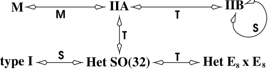
Figure B.1: Some of the dualities among the various string theories and M theory.

Appendix C Scaling of transition curves and equations of states

C.1 Summary

In the subsequent sections, we will tabulate the scaling of the transition curves and equations of states for the phase diagrams studied in the text. The systematic derivation of these formulae can be found in [2, 3, 4]. Note that we use a uniform labeling scheme across the SYM diagrams.

C.2 SYM 1+1

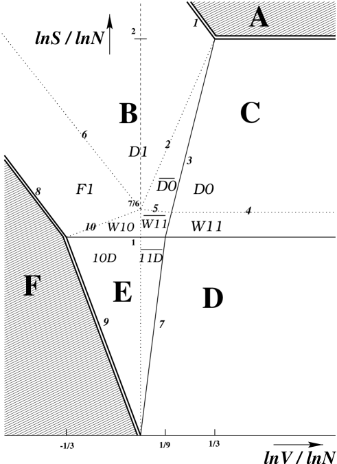
Figure C.1: The thermodynamic phase diagram of $1+1$d SYM. .

Equations of state of bulk phases for $1+1$d ($p=1$) SYM (Figure C.1)

Phase A:	$E\sim\left(\frac{R_{11}}{N}\frac{1}{{\it l}_{{\rm pl}}^{2}}\right)VN^{(p-2)/p}S^{(p+1)/p}\ .$
Phase B:	$E\sim\frac{R_{11}}{{\it l}_{{\rm pl}}^{2}}\left(\frac{S^{2}}{N}\right)^{(7-p)/(9-p)}V^{2p/(9-p)}\ .$
Phase C:	$E\sim\left(\frac{R_{11}}{N}\frac{1}{{\it l}_{{\rm pl}}^{2}}\right)S^{14/9}N^{2/9}\ .$
Phase D:	$E\sim\left(\frac{R_{11}}{N}\frac{1}{{\it l}_{{\rm pl}}^{2}}\right)S^{16/9}\ .$
Phase E:	$E\sim\left(\frac{R_{11}}{N}\frac{1}{{\it l}_{{\rm pl}}^{2}}\right)V^{2p/(9-p)}S^{2(8-p)/(9-p)}\ .$
Phase F:	$E\sim\left(\frac{R_{11}}{N}\frac{1}{{\it l}_{{\rm pl}}^{2}}\right)VS^{2}\ .$

Scaling of transition curves for $1+1$d ($p=1$) SYM

Curve 1:	$S\sim N^{(6-p)/(3-p)}V^{-3p/(3-p)}\ .$
Curve 2:	$S\sim N^{(8-p)/(7-p)}V^{3(6-p)/(7-p)}\ .$
Curve 3:	$S\sim V^{9/2}N^{1/2}\ .$
Curve 4:	$S\sim N^{8/7}\ .$
Curve 5:	$S\sim N^{(8-p)/(7-p)}V^{p/(p-7)}\ .$
Curve 6:	$S\sim N^{(8-p)/(7-p)}V^{3p/(p-3)}\ .$
Curve 7:	$S\sim V^{9}\ .$
Curve 8:	$S\sim V^{-3/2}N^{1/2}\ .$
Curve 9:	$S\sim V^{-3}\ .$
Curve 10:	$S\sim V^{1/2}N^{7/6}\ .$

C.3 SYM 2+1

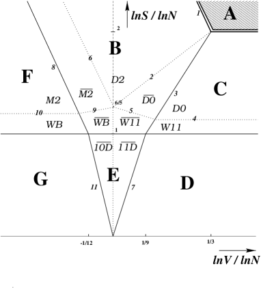
Figure C.2: The thermodynamic phase diagram of $2+1$d SYM. .

Equations of state of bulk phases for $2+1$d SYM (Figure C.2)

Phases A-E:	As in Section C.2 with $p=2$
Phase F:	$E\sim\left(\frac{R_{11}}{N}\frac{1}{{\it l}_{{\rm pl}}^{2}}\right)VS^{3/2}N^{1/4}\ .$
Phase G:	$E\sim\left(\frac{R_{11}}{N}\frac{1}{{\it l}_{{\rm pl}}^{2}}\right)VS^{7/4}\ .$

Scaling of transition curves for $2+1$d SYM

Curves 1-7:	As in Section C.2 with $p=2$
Curve 8:	$S\sim V^{-6}N^{1/2}\ .$
Curve 9:	$S\sim V^{3/10}N^{6/5}\ .$
Curve 10:	$S\sim N^{7/6}\ .$
Curve 11:	$S\sim V^{-12}\ .$

C.4 SYM 3+1

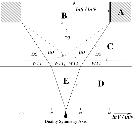
Figure C.3: The thermodynamic phase diagram of $3+1$d SYM. .

Equations of states and scaling of transition curves for $3+1$d SYM (see Figure C.3) are tabulated in Section C.2 with $p=3$.

C.5 $(2,0)$ on $T^{4}\times S^{1}$

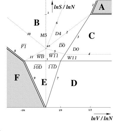
Figure C.4: The thermodynamic phase diagram of the $(2,0)$ on $T^{4}\times S^{1}$. .

Equations of states of bulk phases for $4+1$d SYM (Figure C.4)

Phases A-E:	As in Section C.2 with $p=4$
Phase F:	$E\sim\frac{R_{11}}{{\it l}_{{\rm pl}}^{2}}N^{-1}S^{2}V^{4}\ .$

Scaling of transition curves for $4+1$d SYM

Curves 1-7:	As in Section C.2 with $p=4$
Curve 8:	$S\sim V^{-3}N^{1/2}\ .$
Curve 9:	$S\sim V^{-6}\ .$
Curve 10:	$S\sim V^{-3}N^{4/3}\ .$
Curve 11:	$S\sim V^{2}N^{4/3}\ .$

C.6 $(2,0)$ on $T^{5}$

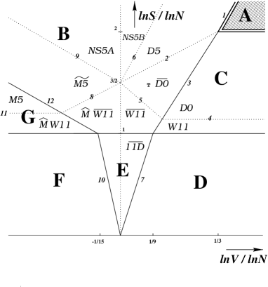
Figure C.5: The thermodynamic phase diagram of the $(2,0)$ on $T^{5}$. .

Equations of states of bulk phases for $5+1$d SYM (Figure C.5)

Phases A-E:	As in Section C.2 with $p=5$
Phase F:	$E\sim\frac{R_{11}}{{\it l}_{{\rm pl}}^{2}}N^{-1}V^{4}S^{8/5}\ .$
Phase G:	$E\sim\frac{R_{11}}{{\it l}_{{\rm pl}}^{2}}S^{6/5}V^{4}N^{-3/5}\ .$

Scaling of transition curves for $5+1$d SYM

Curves 1-7:	As in Section C.2 with $p=5$
Curve 8:	$S\sim V^{3/2}N^{3/2}\ .$
Curve 9:	$S\sim V^{-15/2}N^{3/2}\ .$
Curve 10:	$S\sim V^{-15}\ .$
Curve 11:	$S\sim N^{4/3}\ .$
Curve 12:	$S\sim V^{-15/2}N^{1/2}\ .$

C.7 SYM 6+1

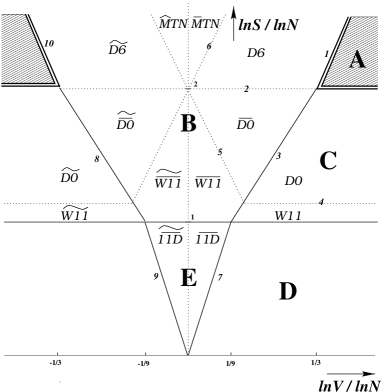
Figure C.6: The thermodynamic phase diagram of the D6 system. .

Equations of states of bulk phases for $6+1$d SYM (Figure C.4) are as in Section C.2 with $p=6$.

Scaling of transition curves for $6+1$d SYM

Curves 1-7:	As in Section C.2 with $p=6$
Curve 8:	$S\sim V^{-9/2}N^{1/2}\ .$
Curve 9:	$S\sim V^{-9}\ .$
Curve 10:	$S\sim V^{-6}\ .$

C.8 Little strings with winding charge

Figure C.7: The thermodynamic phase diagram of D1D5 system. .

Equations of states of bulk phases for D1D5 system (Figure C.7)

Phases A and B:	$E=\frac{S^{2}}{8\pi^{2}kR_{5}}\ .$
Phase C:	$E\sim\frac{g_{6}}{R_{5}}\left(\frac{S}{k^{1/2}}\right)^{3}\ .$

Scaling of transition curves for the D1D5 system

Curve 1:	$S\sim g_{6}^{-1/2}k^{3/4}\ .$
Curve 2:	$S\sim g_{6}^{1/2}k^{3/4}q^{1/2}\ .$
Curve 3:	$S\sim k^{2/3}q^{1/3}\ .$
Curve 4:	$S\sim k^{2/3}q^{-1/6}\ .$
Curve 5:	$S\sim g_{6}^{1/2}k^{3/4}q^{-1/4}\ .$
Curve 6:	$S\sim g_{6}^{-1}k^{3/4}q^{-1/4}\ .$
Curve 7:	$S\sim g_{6}^{-1}k^{1/2}\ .$

Appendix D The $(2,0)$ theory on $T_{4}/Z_{2}\times S^{1}$

Inspired by the discussion regarding the phase structure of the $(2,0)$ on $T^{4}\times S^{1}$, we further consider the phase structure of this theory on $T^{4}/Z_{2}\times S^{1}$. This corresponds to a corner in the moduli space of $K3\times S^{1}$; particularly, in addition to considering a square $T^{4}$, we will be ignoring phase dynamics associated with the $16\times 4$ moduli that blow up the fixed points [94]. Our parameter space is again two dimensional, entropy $S$ and the volume of the $T^{4}$. There are only two novelties that arise, both leaving the global structure of the phase diagram unchanged, modifying only the interpretation of the various patches of geometry.

The first change arises from the effect of the orbifold on the duality transformations; we will obviously be driven into the other branch of the web of dualities that converge onto M theory (c.f. [95]). We proceed from the $\overline{11D}$ phase of the previous discussion, upward and counter- clockwise on the phase diagram. We have M theory on a light-cone circle times $T^{4}/Z_{2}$. We reduce on $R_{11}$ to D0 branes in IIA living on the $T^{4}/Z_{2}$. Under this orbifold, the massless spectrum has positive parity eigenvalue. We T dualize on $T^{4}$, getting to the patch of $D4$ branes in IIA wrapped on $T^{4}/Z_{2}$. We remind the reader of the transformation

$$T_{(4)}\beta_{(4)}T_{(4)}^{-1}=\beta_{(4)}\ ,$$ (D.1)

where we have used the properties of the reflection operator on the spinors

$$\beta_{i}=\Gamma\Gamma^{i}\quad,\qquad\beta_{i}^{2}=(-1)^{F_{L}}\quad,\qquad\left\{\beta_{i},\beta_{j}\right\}=0\ ,$$ (D.2)

with the T duality operation reflecting the left moving spinors only. Here, $(-1)^{F_{L}}$ is the left moving fermion operator. We then M lift to M5 branes in $\widetilde{M}$ theory on $T^{4}/Z_{2}\times S^{1}$. Next, we have to apply the chain of dualities $M,T_{(3)},S$. From the M reduction we obtain $\widetilde{D4}$ branes on $T^{3}/(-1)^{F_{L}}\Omega$. This is because the M reduction along an orbifold direction yields the twist eigenvalues for the massless spectrum

$$g_{\mu\nu}\ +;\ \ \phi\ +;\ \ B_{\mu\nu}\ -;\ \ C^{(1)}\ -;\ \ C^{(3)}\ +\ ,$$ (D.3)

while the world-sheet parity operator $\Omega$ acts on this spectrum as

$$g_{\mu\nu}\ +;\ \phi+;\ B_{\mu\nu}\ -;\ C^{(1),(2),(5),(6)}\ +;\ C^{(0),(3),(4),(7),(8)}\ -\ ,$$ (D.4)

and the action of $(-1)^{F_{L}}$ yields

$$\rm NSNS\ +\quad;\qquad RR-\ .$$ (D.5)

The T duality on $T^{3}$ brings us to $D1$ branes in IIB theory on $S^{1}\times T^{3}/\Omega$, which is type I theory on $S^{1}\times T^{3}$. This is because

$$T_{(3)}\beta_{(3)}(-1)^{F_{L}}\Omega T_{(3)}^{-1}=(-1)^{F_{L}}\Omega\ .$$ (D.6)

Finally, the S duality culminates in the geometry of $N$ black Heterotic strings smeared on the $T^{3}$. The Horowitz-Polchinski correspondence curve patches this phase onto that of the Heterotic Matrix string phase. We thus verify the following previous suggestions [63, 64, 65, 96] from the perspective of Maldacena’s conjecture:

• Heterotic Matrix string theory emerges in the UV of the $(2,0)$ theory.

• Heterotic Matrix strings can be described via the $O(N)$ SYM of type I D strings

The structure of the phase diagram has not changed, but the labeling of some of the phases has. The additional symmetry structure of the orbifold background entered our discussion trivially; the critical behaviors are unaffected.

To complete the discussion, we need to address a second change to the $T^{4}$ compactification. The localization transitions are of a somewhat different nature than the ones encountered earlier. Localized black geometries on orbifold backgrounds are unstable toward collapse toward the nearest fixed point; by virtue of being above extremality, there are static forces, and by virtue of the symmetry structure of the orbifold, there is no balance of forces as in the toroidal case. It is then most probable that the localized D0 branes sit at the orbifold points, with their black horizons surrounding the singularity. The most natural geometry is the one corresponding to 16 black D0 geometries distributed among the singularities, yielding a non-singular geometry outside the horizons.

Appendix E Calculation of the Potential

We need to evaluate

$$\mathcal{V}\equiv\left<\frac{\left\{(\partial_{+}X_{r})^{2}(\partial_{-}X_{r})^{2}-\left[(\partial_{+}X_{r})^{2}+(\partial_{-}X_{r})^{2}\right](\partial_{+}X_{r}.\partial_{-}X_{r})\right\}}{\left(X_{r}^{2}\right)^{D/2}}\right>\ ,$$ (E.1)

in the finite temperature vacuum of the SYM. Let subscripts $(123456)$ denote the argument of $X$, e.g. $X_{1}\equiv X(\sigma_{1})$. Writing $X_{r}\equiv X_{5}-X_{6}$, we will encounter in the numerator only factors of the form

$$\partial_{\alpha}X^{i}_{1}\partial_{\alpha}X^{i}_{2}\partial_{\beta}X^{j}_{3}\partial_{\gamma}X^{j}_{4}\ ,$$ (E.2)

with the target indices $i$, $j$ summed over; $\alpha$, $\beta$, $\gamma$ are worldsheet indices $\pm$; and the labels $(1234)$ are set equal to $5$ and $6$ in various ways. By expanding the numerator of equation (E.1), we get $3\times 16$ terms of the form claimed. We can write our desired ‘monomial’ (E.2) as

$$\partial_{\alpha}^{1}\partial_{\alpha}^{2}\partial_{\beta}^{3}\partial_{\gamma}^{4}\left<\frac{X_{1}^{i}X_{2}^{i}X_{3}^{j}X_{4}^{j}}{((X_{5}-X_{6})^{2})^{D/2}}\right>\ .$$ (E.3)

Consider

$$\left<\frac{X_{1}^{i}X_{2}^{i}X_{3}^{j}X_{4}^{j}}{((X_{5}-X_{6})^{2})^{D/2}}\right> = \frac{\pi^{-d/2}}{\Gamma(D/2)}\int_{0}^{\infty}ds\ \int d^{d}p\ s^{(D/2)-1}e^{-p^{2}}\delta_{1}^{i}\delta_{2}^{i}\delta_{3}^{j}\delta_{4}^{j}\left<e^{\int\tilde{J}.X}\right>$$ (E.4)

$$= \frac{\pi^{-d/2}}{\Gamma(D/2)}\int_{0}^{\infty}ds\ \int d^{d}p\ s^{(D/2)-1}e^{-p^{2}}\delta_{1}^{i}\delta_{2}^{i}\delta_{3}^{j}\delta_{4}^{j}e^{\Delta}$$

where

$$\tilde{J^{i}}\equiv J^{i}+2i\sqrt{s}(\delta(\sigma-\sigma_{5})-\delta(\sigma-\sigma_{6}))p^{i}$$ (E.5)

and

$$\Delta\equiv\frac{1}{4}\int\tilde{J}K\tilde{J}=\frac{1}{4}\int JKJ+i\sqrt{s}\int J.pK_{x}-2sp^{2}f^{2}$$ (E.6)

We have defined

$$K_{x}\equiv K_{x5}-K_{x6}$$ (E.7)

$$f^{2}\equiv K-K_{56}$$ (E.8)

Here $K_{ab}$ means $K(a-b)$, the Green’s function of the two dimensional Laplacian

$$K_{ab}\equiv-{\alpha^{\prime}}\langle X_{a}X_{b}\rangle\ ,$$ (E.9)

and $K\equiv K_{aa}$. The rest is an exercise in combinatorics, making use of

$$\delta_{a}^{i}e^{\Delta}=\left[\frac{1}{2}\int G_{ax}J^{i}+i\sqrt{s}p^{i}K_{a}\right]e^{\Delta}$$ (E.10)

where the $x$ subscript is integrated over and it is implied to be the argument of the $J$ as well. Denoting the number of polarizations in the Lorentz indices by $d$, we get

$$\left<\frac{X_{1}^{i}X_{2}^{i}X_{3}^{j}X_{4}^{j}}{((X_{5}-X_{6})^{2})^{D/2}}\right> = \frac{\pi^{-d/2}}{\Gamma(D/2)}\int ds\int d^{d}p\ e^{-p^{2}}e^{-2sp^{2}f^{2}}$$ (E.11)

$$\times \left[T_{1}s^{(D/2)-1}-\frac{1}{2}p^{2}s^{D/2}T_{2}+(p^{2})^{2}s^{(D/2)+1}T_{4}\right]$$

where we have defined

$$T_{1}\equiv\frac{d^{2}}{4}K_{12}K_{34}+\frac{d}{4}K_{13}K_{24}+\frac{d}{4}K_{23}K_{14}$$ (E.12)

$$T_{2}\equiv dK_{1}K_{2}K_{34}+dK_{3}K_{4}K_{12}+K_{1}K_{3}K_{24}+K_{1}K_{4}K_{23}+K_{2}K_{3}K_{14}+K_{2}K_{4}K_{13}$$ (E.13)

$$T_{4}\equiv K_{1}K_{2}K_{3}K_{4}$$ (E.14)

Evaluating the $s$ integral, we get

$$\left<\frac{X_{1}^{i}X_{2}^{i}X_{3}^{j}X_{4}^{j}}{((X_{5}-X_{6})^{2})^{D/2}}\right>=\frac{\pi^{-d/2}}{2^{D/2}(f^{2})^{D/2}}\int d^{d}p\ e^{-p^{2}}(p^{2})^{-D/2}\left[T_{1}-\frac{D}{8f^{2}}T_{2}+\frac{(D+2)D}{16(f^{2})^{2}}T_{4}\right]$$ (E.15)

Evaluating the $p$ integrals, we get

$$\left<\frac{X_{1}^{i}X_{2}^{i}X_{3}^{j}X_{4}^{j}}{((X_{5}-X_{6})^{2})^{D/2}}\right>=\frac{\pi^{-d/2}}{2^{(D/2)+1}(f^{2})^{D/2}}\Omega_{d-1}\Gamma\left(\frac{d-D}{2}\right)\left[T_{1}-\frac{D}{8f^{2}}T_{2}+\frac{(D+2)D}{16(f^{2})^{2}}T_{4}\right]$$ (E.16)

where $\Omega_{d-1}$ is the volume of the $d-1$ unit sphere.

Going back to (E.3), we need to differentiate $T_{1}$, $T_{2}$ and $T_{4}$, according to the map $1234\rightarrow\alpha\alpha\beta\gamma$. Let us denote the derivatives by superscripts on the $K$’s. We then have

$$T_{1}^{\alpha\alpha\beta\gamma}=\frac{d^{2}}{4}K_{12}^{\alpha\alpha}K_{34}^{\beta\gamma}+\frac{d}{4}K_{13}^{\alpha\beta}K_{24}^{\alpha\gamma}+\frac{d}{4}K_{23}^{\alpha\beta}K_{14}^{\alpha\gamma}\ ,$$ (E.17)

$$T_{2}^{\alpha\alpha\beta\gamma} = dK_{1}^{\alpha}K_{2}^{\alpha}K_{34}^{\beta\gamma}+dK_{3}^{\beta}K_{4}^{\gamma}K_{12}^{\alpha\alpha}+K_{1}^{\alpha}K_{3}^{\beta}K_{24}^{\alpha\gamma}$$ (E.18)

$$+ K_{1}^{\alpha}K_{4}^{\gamma}K_{23}^{\alpha\beta}+K_{2}^{\alpha}K_{3}^{\beta}K_{14}^{\alpha\gamma}+K_{2}^{\alpha}K_{4}^{\gamma}K_{13}^{\alpha\beta}\ ,$$

$$T_{4}^{\alpha\alpha\beta\gamma}=K_{1}^{\alpha}K_{2}^{\alpha}K_{3}^{\beta}K_{4}^{\gamma}\ .$$ (E.19)

We have used here the translational invariance and evenness of the Green’s function to interpret the derivatives as differentiations with respect to the argument $i-j$ of the Green’s functions (and therefore note some flip of signs); furthermore, we assume that $K$, $K^{\alpha}$ and $K^{\alpha\beta}$ are zero, i.e. because of subtraction of the zero temperature limits, or throwing away bubble diagrams. This, it turns out, is not necessary for the potential we calculate, since all expressions would have come out as differences, say $K^{\alpha\beta}_{12}-K^{\alpha\beta}$; it is just convenient for notational purposes to throw them out from the start. We also note the identities $K^{\alpha\beta}_{12}=K^{\alpha\beta}_{21}$ and $K^{\alpha}_{5}=-K_{56}^{\alpha}=K^{\alpha}_{6}$. For each term in equations (E.17)-(E.19), we have 16 terms associated with taking a map from $(1234)$ to a sequence of $5$’s and $6$’s. This combinatorics yields

$$\left<\frac{\partial_{\alpha}X_{r}^{i}\partial_{\alpha}X_{r}^{i}\partial_{\beta}X_{r}^{j}\partial_{\gamma}X_{r}^{j}}{\left(X_{r}^{2}\right)^{D/2}}\right>\simeq\frac{K_{56}^{\alpha\beta}K_{56}^{\alpha\gamma}+\frac{d}{2}K_{56}^{\alpha\alpha}K_{56}^{\beta\gamma}}{(-K_{56})^{D/2}}\ .$$ (E.20)

Note that $T_{2}$ and $T_{4}$ cancelled; we have also dropped numerical coefficients. There are three terms in (E.1) of this type; this yields

$$\mathcal{V}\simeq\frac{K_{56}^{+-}K_{56}^{+-}+\frac{d}{2}K_{56}^{++}K_{56}^{--}-\left(\frac{d}{2}+1\right)\left(K_{56}^{++}K_{56}^{+-}+K_{56}^{--}K_{56}^{+-}\right)}{(-K_{56})^{D/2}}\ .$$ (E.21)

Using the equation of motion (delta singularity subtracted) $K_{56}^{+-}=0$, we get

$$\mathcal{V}\simeq\frac{K_{56}^{++}K_{56}^{--}}{(-K_{56})^{D/2}}\ .$$ (E.22)

Using Euclidean time $i\tau=t$, we have $\sigma^{\pm}=\sigma\pm t=z,\bar{z}$; finally, we get for equation (4.26)

$$V_{12}=\alpha_{D}g_{s}^{2}\frac{{\it l}_{{{\it str}}}^{5-p}}{R_{+}}\frac{K^{zz}_{12}K^{\bar{z}\bar{z}}_{12}}{\left(-K_{12}\right)^{D/2}}.$$ (E.23)

Appendix F Longitudinal momentum transfer effects

Consider the scattering of two wound strings in IIB theory with winding number exchange. We will find that, in the regime of small momentum transfer, the interaction is Coulombic for resonances involving low enough winding number exchange, and much weaker otherwise; furthermore, the Coulombic interaction is winding number independent, and the cumulative strength of this potential suggests modifying the Matrix string potential by a factor of $N/S$ for $N>S$.

For simplicity, consider the polarizations of the external states to be that of the dilaton, and T-dualize the momentum in the compact direction to winding number. The resulting four string amplitude is given by [97]

$$A_{m}\sim K_{\alpha\beta\gamma\delta}K^{\alpha\beta\gamma\delta}\frac{\Gamma(-S{\alpha^{\prime}}/4)\Gamma(-T{\alpha^{\prime}}/4)\Gamma(-U{\alpha^{\prime}}/4)}{\Gamma(1+S{\alpha^{\prime}}/4)\Gamma(1+T{\alpha^{\prime}}/4)\Gamma(1+U{\alpha^{\prime}}/4)}\ ,$$ (F.1)

where $S\equiv-(k_{1}+k_{2})^{2}$, $T\equiv-(k_{2}+k_{3})^{2}$, $U\equiv-(k_{1}+k_{3})^{2}$, with $S+T+U=0$, and

$$K^{\alpha\beta\gamma\delta} = -\frac{1}{2}\left(ST\eta^{\alpha\gamma}\eta^{\beta\delta}+SU\eta^{\beta\gamma}\eta^{\alpha\delta}+TU\eta^{\alpha\beta}\eta^{\gamma\delta}\right)$$ (F.2)

$$+ S\left(k_{4}^{\alpha}k_{2}^{\gamma}\eta^{\beta\delta}+k_{3}^{\beta}k_{1}^{\delta}\eta^{\alpha\gamma}+k_{3}^{\alpha}k_{2}^{\delta}\eta^{\beta\gamma}+k_{4}^{\beta}k_{1}^{\gamma}\eta^{\alpha\delta}\right)$$

$$+ T\left(k_{4}^{\gamma}k_{2}^{\alpha}\eta^{\beta\delta}+k_{3}^{\delta}k_{1}^{\beta}\eta^{\alpha\gamma}+k_{4}^{\beta}k_{3}^{\alpha}\eta^{\gamma\delta}+k_{1}^{\gamma}k_{2}^{\delta}\eta^{\alpha\beta}\right)$$

$$+ U\left(k_{2}^{\alpha}k_{3}^{\delta}\eta^{\beta\gamma}+k_{4}^{\gamma}k_{1}^{\beta}\eta^{\alpha\delta}+k_{4}^{\alpha}k_{3}^{\beta}\eta^{\gamma\delta}+k_{2}^{\gamma}k_{1}^{\delta}\eta^{\alpha\beta}\right)\ .$$

This gives the amplitude

$$A_{m}\sim\left[(S+T)^{4}+S^{4}+T^{4}\right]\frac{\Gamma(-S{\alpha^{\prime}}/4)\Gamma(-T{\alpha^{\prime}}/4)\Gamma(-U{\alpha^{\prime}}/4)}{\Gamma(1+S{\alpha^{\prime}}/4)\Gamma(1+T{\alpha^{\prime}}/4)\Gamma(1+U{\alpha^{\prime}}/4)}\ .$$ (F.3)

We want to accord winding $n_{1}$, $n_{2}$, $n_{3}$ and $n_{4}$ to the four strings, on a circle of radius $R$; without any momenta along this cycle, we can extract easily this process from the amplitude above by

$$s=S+M^{2}\ ,$$ (F.4)

$$t=T+m^{2}\equiv-q^{2}\ ,$$ (F.5)

with

$$M^{2}\equiv\left(\frac{R(n_{1}+n_{2})}{{\alpha^{\prime}}}\right)^{2}\ ,$$ (F.6)

$$m^{2}\equiv\left(\frac{R(n_{3}-n_{2})}{{\alpha^{\prime}}}\right)^{2}\ .$$ (F.7)

For large $m_{1},m_{2}$, and small $m$, $q^{2}$ is the spatial momentum transfer between the strings in the center-of-mass frame. Thus $M\gg m$, and we are in the non-relativistic regime $E_{cm}^{2}\gg q^{2}$. From equations (F.4) and (F.5), we see that $S\gg T$. Using this and the identities $\Gamma(z)\Gamma(1-z)\sin(\pi z)=\pi$ and $\Gamma(1+z)=z\Gamma(z)$, one obtains the amplitude

$$A_{m}\sim(s-M^{2})^{2}\sin\left(\pi(q^{2}+m^{2}){\alpha^{\prime}}/4\right)\left(\Gamma((q^{2}+m^{2}){\alpha^{\prime}}/4)\right)^{2}\ .$$ (F.8)

In the energetic regime considered,

$$s-M^{2}\sim m_{1}m_{2}v_{rel}^{2}\equiv\sqrt{{\cal T}}\ ,$$ (F.9)

where $v_{rel}$ is the relative velocity of strings $1$ and $2$ in the lab frame.

Equation (F.8) has poles at $q^{2}+m^{2}=4n/{\alpha^{\prime}}$ with $n\leq 0$. We consider scattering processes probing distances $r$ much larger than the string scale, $q_{max}\sim 1/r\ll 1/{\it l}_{{{\it str}}}$; we also assume that it is possible to have $R\ll{\it l}_{{{\it str}}}$, which we will see is necessary. Given that these poles space the masses of the resonances by the string scale, the dominant term to the amplitude is the one corresponding to the exchange of a wound ground state, i.e. the $n=0$ pole. Measuring quantities in string units, the amplitude then becomes

$$A_{m}\sim{\cal T}\frac{\sin(q^{2}+m^{2})}{\left(q^{2}+m^{2}\right)^{2}}\ .$$ (F.10)

The effective potential between the strings is the Fourier transform of this expression with respect to $q$. Let us consider various limits. Take $m\ll q$; we then have $m\ll 1$. The amplitude becomes

$$A_{m}^{(1)}\sim\frac{{\cal T}}{q^{2}}\ .$$ (F.11)

Next consider $m\gg q$, but $m\ll 1$. The amplitude becomes

$$A_{m}^{(2)}\sim\frac{{\cal T}}{q^{2}+m^{2}}\ .$$ (F.12)

Finally, for $m\gg q$ and $m\gg 1$, we have a constant

$$A_{m}^{(3)}\sim{\cal T}\frac{\sin m^{2}}{m^{4}}\ .$$ (F.13)

The effective potentials are then ($d\equiv 9-p$)

$$V_{eff}^{(1)}\sim\int d^{d}q\ e^{iq.x}A_{m}^{(1)}\sim\frac{T}{r^{d-2}}\ .$$ (F.14)

The result is a Coulomb potential, independent of $m$. The second case gives

$$V_{eff}^{(2)}\sim T\left(2\pi\right)^{d/2}\left(\frac{m}{r}\right)^{d/2-1}\sqrt{\frac{\pi}{2mr}}e^{-mr}\ ,$$ (F.15)

which is weaker than $V_{eff}^{(1)}$ since we have $mr\gg 1$. Finally, we have

$$V_{eff}^{(3)}\sim T\frac{\sin m^{2}}{m^{4}}\frac{1}{r^{d}}\ .$$ (F.16)

In addition to a larger power in $r$, we have $m\gg 1$; this interaction is much weaker than (F.14),(F.15), especially after averaging over a range of winding transfers $m$.

We conclude that, for $mr=Rr(n_{3}-n_{2})/{\alpha^{\prime}}\ll 1$, we have a Coulombic potential independent of the winding exchange $m$; for $mr\gg 1$, we have much weaker potentials. This implies that in a gas of winding strings bound in a ball of size at most of order the string scale, the dominant potential is Coulombic with a multiplicative factor given by $w_{0}\equiv{\alpha^{\prime}}/(Rr)$, provided a mechanism restricts winding exchange processes to $n_{3}-n_{2}\ll n_{1}+n_{2}$.

The S-dual of this amplitude describes the scattering of wound D-strings at strong coupling, with winding number exchange. Under a further T duality, and lifting to M theory, this amplitude encodes a good measure of the effects of longitudinal momentum exchange in the problem of a self-interacting Matrix string. The bound on the winding number translates in our language to

$$w_{0}=\frac{{\bar{\alpha}}^{\prime}\bar{g}_{s}}{\Sigma r}=\frac{R_{11}}{r}\sim\frac{N}{S}\ ,$$ (F.17)

i.e. the resolution in the longitudinal direction. We also note that, under this chain of dualities, the string scale used to set a bound on the impact parameter $r$ transforms as ${\alpha^{\prime}}\rightarrow{\alpha^{\prime}}$, where the latter string scale is that of the Matrix string. This justifies our implied equivalence between the scale of $r$ and that of the size of the black hole.

In the single Matrix string case we study, we saw that regions of size $N/S$ were strongly correlated and ‘rigid’ in a statistical sense. The self-interaction of the large string will then involve processes of coherent exchange of D-string winding up to the winding number $N/S\ll N$. For larger winding, the D-string is not coherent; one expects a suppression both from the emission vertex and from the highly off-shell propagator. We saw above that all such processes, up to $N/S$, are of equal strength and scale Coulombically. This implies that the potential between the string strands calculated from the DBI expansion must be enhanced by a factor of $N/S$ for $N>S$, and justifies the scaling arguments used in Section 4.3.4.

Bibliography

- [1]
- [2] M. Li, E. Martinec, and V. Sahakian, “Black holes and the SYM phase diagram,” hep-th/9809061.
- [3] E. Martinec and V. Sahakian, “Black holes and the Super Yang-Mills phase diagram. 2,” hep-th/9810224.
- [4] E. Martinec and V. Sahakian, “Black holes and five-brane thermodynamics,” hep-th/9901135.
- [5] A. Strominger and C. Vafa, “Microscopic origin of the Bekenstein-Hawking entropy,” Phys. Lett. B379 (1996) 99–104, hep-th/9601029.
- [6] J. M. Maldacena, “Black holes in string theory,” hep-th/9607235.
- [7] E. Witten, “String theory dynamics in various dimensions,” Nucl. Phys. B443 (1995) 85–126, hep-th/9503124.
- [8] C. M. Hull and P. K. Townsend, “Unity of superstring dualities,” Nucl. Phys. B438 (1995) 109–137, hep-th/9410167.
- [9] T. Banks, W. Fischler, S. H. Shenker, and L. Susskind, “M theory as a Matrix model: A conjecture,” Phys. Rev. D55 (1997) 5112–5128, hep-th/9610043.
- [10] J. Maldacena, “The large N limit of superconformal field theories and supergravity,” hep-th/9711200.
- [11] L. Susskind, “Another conjecture about M(atrix) theory,” hep-th/9704080.
- [12] E. Witten, “Anti-de Sitter space and holography,” hep-th/9802150.
- [13] S. S. Gubser, I. R. Klebanov, and A. M. Polyakov, “Gauge theory correlators from noncritical string theory,” Phys. Lett. B428 (1998) 105, hep-th/9802109.
- [14] N. Itzhaki, J. M. Maldacena, J. Sonnenschein, and S. Yankielowicz, “Supergravity and the large N limit of theories with sixteen supercharges,” Phys. Rev. D58 (1998) 046004, hep-th/9802042.
- [15] A. Sen, “Unification of string dualities,” Nucl. Phys. Proc. Suppl. 58 (1997) 5, hep-th/9609176.
- [16] A. Sen, “An introduction to nonperturbative string theory,” hep-th/9802051.
- [17] F. Gliozzi, J. Scherk, and D. Olive, “Supergravity and the spinor dual model,” Phys. Lett. 65B (1976) 282.
- [18] C. G. Callan, E. J. Martinec, M. J. Perry, and D. Friedan, “Strings in background fields,” Nucl. Phys. B262 (1985) 593.
- [19] G. T. Horowitz and A. Strominger, “Black strings and p-branes,” Nucl. Phys. B360 (1991) 197–209.
- [20] M. J. Duff, R. R. Khuri, and J. X. Lu, “String solitons,” Phys. Rept. 259 (1995) 213–326, hep-th/9412184.
- [21] I. R. Klebanov and A. A. Tseytlin, “Entropy of near extremal black p-branes,” Nucl. Phys. B475 (1996) 164–178, hep-th/9604089.
- [22] M. J. Duff, H. Lu, and C. N. Pope, “The black branes of M theory,” Phys. Lett. B382 (1996) 73–80, hep-th/9604052.
- [23] L. Brink, J. H. Schwarz, and J. Scherk, “Supersymmetric Yang-Mills theories,” Nucl. Phys. B121 (1977) 77.
- [24] J. Polchinski, “Tasi lectures on D-branes,” hep-th/9611050.
- [25] A. Strominger, “Open p-branes,” Phys. Lett. B383 (1996) 44–47, hep-th/9512059.
- [26] R. Dijkgraaf, E. Verlinde, and H. Verlinde, “5-d black holes and Matrix strings,” Nucl. Phys. B506 (1997) 121, hep-th/9704018.
- [27] R. Dijkgraaf, E. Verlinde, and H. Verlinde, “BPS spectrum of the five-brane and black hole entropy,” Nucl. Phys. B486 (1997) 77–88, hep-th/9603126.
- [28] O. Ganor and L. Motl, “Equations of the (2,0) theory and knitted five-branes,” JHEP 05 (1998) 009, hep-th/9803108.
- [29] N. Seiberg, “New theories in six-dimensions and Matrix description of m theory on t**5 and t**5 / z(2),” Phys. Lett. B408 (1997) 98–104, hep-th/9705221.
- [30] O. Aharony, S. S. Gubser, J. Maldacena, H. Ooguri, and Y. Oz, “Large N field theories, string theory and gravity,” hep-th/9905111.
- [31] N. Seiberg, “Why is the Matrix model correct?,” Phys. Rev. Lett. 79 (1997) 3577–3580, hep-th/9710009.
- [32] G. T. Horowitz and E. J. Martinec, “Comments on black holes in Matrix theory,” Phys. Rev. D57 (1998) 4935–4941, hep-th/9710217.
- [33] I. R. Klebanov and L. Susskind, “Schwarzschild black holes in various dimensions from Matrix theory,” Phys. Lett. B416 (1998) 62, hep-th/9709108.
- [34] M. Li and E. Martinec, “Probing Matrix black holes,” hep-th/9801070.
- [35] L. Motl, “Proposals on nonperturbative superstring interactions,” hep-th/9701025.
- [36] R. Dijkgraaf, E. Verlinde, and H. Verlinde, “Matrix string theory,” Nucl. Phys. B500 (1997) 43, hep-th/9703030.
- [37] E. Witten, “Bound states of strings and p-branes,” Nucl. Phys. B460 (1996) 335–350, hep-th/9510135.
- [38] Z. Guralnik and S. Ramgoolam, “Torons and D-brane bound states,” Nucl. Phys. B499 (1997) 241, hep-th/9702099.
- [39] O. J. Ganor, S. Ramgoolam, and I. Washington Taylor, “Branes, fluxes and duality in M(atrix) theory,” Nucl. Phys. B492 (1997) 191–204, hep-th/9611202.
- [40] V. Sahakian, “On the bound states of Matrix strings,” hep-th/9710242.
- [41] G. T. Horowitz and J. Polchinski, “A correspondence principle for black holes and strings,” Phys. Rev. D55 (1997) 6189–6197, hep-th/9612146.
- [42] J. L. F. Barbon, I. I. Kogan, and E. Rabinovici, “On stringy thresholds in SYM/AdS thermodynamics,” hep-th/9809033.
- [43] A. Giveon, M. Porrati, and E. Rabinovici, “Target space duality in string theory,” Phys. Rept. 244 (1994) 77–202, hep-th/9401139.
- [44] R. Gregory and R. Laflamme, “The instability of charged black strings and p-branes,” Nucl. Phys. B428 (1994) 399–434, hep-th/9404071.
- [45] R. Gregory and R. Laflamme, “Black strings and p-branes are unstable,” Phys. Rev. Lett. 70 (1993) 2837, hep-th/9301052.
- [46] T. Banks, W. Fischler, I. R. Klebanov, and L. Susskind, “Schwarzschild black holes from Matrix theory,” Phys. Rev. Lett. 80 (1998) 226–229, hep-th/9709091.
- [47] T. Banks, W. Fischler, I. R. Klebanov, and L. Susskind, “Schwarzschild black holes in Matrix theory. 2,” J. High Energy Phys. 01 (1998) 008, hep-th/9711005.
- [48] W. Fischler, E. Halyo, A. Rajaraman, and L. Susskind, “The incredible shrinking torus,” Nucl. Phys. B501 (1997) 409, hep-th/9703102.
- [49] M. Berkooz, M. Rozali, and N. Seiberg, “Matrix description of M theory on and ,” Phys. Lett. B408 (1997) 105–110, hep-th/9704089.
- [50] A. Sen, “D0-branes on and Matrix theory,” Adv. Theor. Math. Phys. 2 (1998) 51, hep-th/9709220.
- [51] I. Brunner and A. Karch, “Matrix description of M theory on ,” Phys. Lett. B416 (1998) 67, hep-th/9707259.
- [52] A. Hanany and G. Lifschytz, “M(atrix) theory on and a M(atrix) theory description of KK monopoles,” Nucl. Phys. B519 (1998) 195, hep-th/9708037.
- [53] A. Losev, G. Moore, and S. L. Shatashvili, “M and m’s,” Nucl. Phys. B522 (1998) 105, hep-th/9707250.
- [54] J. Maldacena and A. Strominger, “AdS(3) black holes and a stringy exclusion principle,” JHEP 12 (1998) 005, hep-th/9804085.
- [55] E. J. Martinec, “Matrix models of AdS gravity,” hep-th/9804111.
- [56] A. Giveon, D. Kutasov, and N. Seiberg, “Comments on string theory on AdS(3),” Adv. Theor. Math. Phys. 2 (1998) 733–780, hep-th/9806194.
- [57] O. Aharony, M. Berkooz, S. Kachru, N. Seiberg, and E. Silverstein, “Matrix description of interacting theories in six dimensions,” Adv. Theor. Math. Phys. 1 (1998) 148–157, hep-th/9707079.
- [58] N. Seiberg and S. Sethi, “Comments on Neveu-Schwarz five-branes,” Adv. Theor. Math. Phys. 1 (1998) 259, hep-th/9708085.
- [59] S. Sethi, “The Matrix formulation of type IIB five-branes,” Nucl. Phys. B523 (1998) 158, hep-th/9710005.
- [60] O. J. Ganor and S. Sethi, “New perspectives on Yang-Mills theories with sixteen supersymmetries,” JHEP 01 (1998) 007, hep-th/9712071.
- [61] C. V. Johnson, “More superstrings from supergravity,” Nucl. Phys. B537 (1999) 129, hep-th/9805047.
- [62] T. Banks and N. Seiberg, “Strings from matrices,” Nucl. Phys. B497 (1997) 41–55, hep-th/9702187.
- [63] M. Berkooz and M. Rozali, “String dualities from Matrix theory,” Nucl. Phys. B516 (1998) 229, hep-th/9705175.
- [64] D.-E. Diaconescu and J. Gomis, “Matrix description of heterotic theory on K3,” Phys. Lett. B433 (1998) 35–42, hep-th/9711105.
- [65] T. Banks and L. Motl, “Heterotic strings from matrices,” JHEP 12 (1997) 004, hep-th/9703218.
- [66] D. A. Lowe, “Heterotic Matrix string theory,” Phys. Lett. B403 (1997) 243–249, hep-th/9704041.
- [67] P. Horava, “Matrix theory and heterotic strings on tori,” Nucl. Phys. B505 (1997) 84, hep-th/9705055.
- [68] L. Susskind and E. Witten, “The holographic bound in Anti-de Sitter space,” hep-th/9805114.
- [69] A. W. Peet and J. Polchinski, “UV / IR relations in AdS dynamics,” hep-th/9809022.
- [70] A. Sen, “T duality of p-branes,” Mod. Phys. Lett. A11 (1996) 827–834, hep-th/9512203.
- [71] E. Martinec and V. Sahakian, work in progress.
- [72] A. Strominger, “Black hole entropy from near horizon microstates,” JHEP 02 (1998) 009, hep-th/9712251.
- [73] J. D. Brown and M. Henneaux, “Central charges in the canonical realization of asymptotic symmetries: An example from three-dimensional gravity,” Commun. Math. Phys. 104 (1986) 207.
- [74] C. Vafa, “Gas of D-branes and Hagedorn density of BPS states,” Nucl. Phys. B463 (1996) 415–419, hep-th/9511088.
- [75] A. Dabholkar and J. A. Harvey, “Nonrenormalization of the superstring tension,” Phys. Rev. Lett. 63 (1989) 478.
- [76] G. T. Horowitz and J. Polchinski, “Selfgravitating fundamental strings,” Phys. Rev. D57 (1998) 2557–2563, hep-th/9707170.
- [77] F. Reif, Statistical Mechanics. McGraw-Hill, 1965.
- [78] R. Hagedorn, “Statistical thermodynamics of strong interactions at high energies,” Nuovo Cim. Suppl. 3 (1965) 147–186.
- [79] J. J. Atick and E. Witten, “The Hagedorn transition and the number of degrees of freedom of string theory,” Nucl. Phys. B310 (1988) 291.
- [80] T. Wynter, “Gauge fields and interactions in Matrix string theory,” Phys. Lett. B415 (1997) 349, hep-th/9709029.
- [81] J. H. Schwarz, “An SL(2,Z) multiplet of type IIB superstrings,” Phys. Lett. B360 (1995) 13–18, hep-th/9508143.
- [82] K. Becker, M. Becker, J. Polchinski, and A. Tseytlin, “Higher order graviton scattering in M(atrix) theory,” Phys. Rev. D56 (1997) 3174–3178, hep-th/9706072.
- [83] E. Keski-Vakkuri and P. Kraus, “Born-Infeld actions from Matrix theory,” Nucl. Phys. B518 (1998) 212, hep-th/9709122.
- [84] N. Goldenfeld, Lectures on phase transitions and the renormalization group. Addison Wesley, 1995.
- [85] P. D. Francesco, P. Mathieu, and D. Senechal, Conformal Field Theory. Springer Verlag, 1997.
- [86] E. Kiritsis, Introduction to Superstring Theory. Leuven University Press, 1998.
- [87] I. S. Gradshteyn and I. M. Ryzhik, Table of integrals, series and products. Academic Press, 1994.
- [88] D. Mitchell and N. Turok, “Statistical mechanics of cosmic strings,” Phys. Rev. Lett. 58 (1987) 1577.
- [89] J. X. Lu, “ADM masses for black strings and p-branes,” Phys. Lett. B313 (1993) 29–34, hep-th/9304159.
- [90] K. S. Narain, “New heterotic string theories in uncompactified dimensions ¡ 10,” Phys. Lett. 169B (1986) 41.
- [91] K. S. Narain, M. H. Sarmadi, and E. Witten, “A note on toroidal compactification of heterotic string theory,” Nucl. Phys. B279 (1987) 369.
- [92] J. H. Schwarz and A. Sen, “Duality symmetries of 4-d heterotic strings,” Phys. Lett. B312 (1993) 105–114, hep-th/9305185.
- [93] J. H. Schwarz and A. Sen, “Duality symmetric actions,” Nucl. Phys. B411 (1994) 35–63, hep-th/9304154.
- [94] P. S. Aspinwall, “K3 surfaces and string duality,” hep-th/9611137.
- [95] J.Polchinski, String Theory, Vol. 2. Cambridge University Press, 1998.
- [96] L. Motl and L. Susskind, “Finite N heterotic Matrix models and discrete light cone quantization,” hep-th/9708083.
- [97] M. Green, J. Schwarz, and E. Witten, Superstring Theory, Vol. I and II. Cambridge University Press, 1987.