DTP 99-37

EHU-FT/9909

hep-th/9906040

AdS/CFT Duals of Topological Black Holes and the Entropy of Zero–Energy States

Roberto Emparan

Department of Mathematical Sciences
University of Durham, Durham DH1 3LE, UK
and

Departamento de Física Teórica
Universidad del País Vasco, Apdo. 644, E-48080, Bilbao, Spain

The horizon of a static black hole in Anti-deSitter space can be spherical, planar, or hyperbolic. The microscopic dynamics of the first two classes of black holes have been extensively discussed recently within the context of the AdS/CFT correspondence. We argue that hyperbolic black holes introduce new and fruitful features in this respect, allowing for more detailed comparisons between the weak and strong coupling regimes. In particular, by focussing on the stress tensor and entropy of some particular states, we identify unexpected increases in the entropy of Super–Yang–Mills theory at strong coupling that are not accompanied by increases in the energy. We describe a highly degenerate state at zero temperature and zero energy density. We also find that the entanglement entropy across a Rindler horizon in exact AdS₅ is larger than might have been expected from the dual SYM theory. Besides, we show that hyperbolic black holes can be described as thermal Rindler states of the dual conformal field theory in flat space.

May 1999

1 Introduction

The correspondence between string theory in Anti-deSitter (AdS) space and conformal field theory (CFT) [1, 2, 3] provides a powerful basis for the study of the microscopic statistical mechanics of black holes. In this framework, a black hole in AdS is described as a thermal state of the dual conformal field theory. The latter is defined on a background geometry that is conformally related to the geometry at the boundary of the AdS space. If we want to work in a regime where the supergravity approximation to string theory is reliable, then the dual CFT has to be strongly coupled. The aim of this paper is to develop the duality for a class of black holes peculiar to AdS space, that will exhibit new and remarkable features.

It is known that the presence of a negative cosmological constant allows for more varied types of horizon geometries than in asymptotically flat situations. In AdS the horizon of a black hole can have positive, zero, or negative curvature. These are spherical, planar or hyperbolic black holes, respectively. In four dimensions it is possible to construct horizons of arbitrary topology by modding out discrete isometry groups. This is the origin of the name “topological black holes.” We keep this name, even if it will be somewhat of a misnomer since we will not be considering identifications under discrete isometries. Nevertheless, that is something that could be implemented in a straightforward manner.

The microscopic study of planar black holes within string theory can be traced back to the discussion in [4] of the statistical mechanics of black D3-branes. As this system is understood now, the planar black hole in AdS₅ is dual to a thermal state of ${\cal N}{=}4$ supersymmetric Yang–Mills (SYM) theory in four dimensional Minkowski space, with gauge group $SU(N)$, in the large $N$ limit and at a large value of the ‘tHooft coupling $g^{2}_{YM}N$. We have very limited knowledge of gauge theory in such a strong coupling regime, but the results that follow from calculations using AdS supergravity appear to be remarkably close to what we are able to compute using free field theory. The AdS₅/SYM pair is the most studied case, but for other dimensions we know that the temperature dependence of the dual field theories is determined by conformal invariance, and this behavior is indeed reproduced by planar black holes [5, 6].

Spherical black holes, on the other hand, present a different qualitative feature, namely, a phase transition at finite temperature [7]. As observed in [3, 6] this phase transition fits in nicely with our expectations of a confining phase at low temperatures for large $N$ theory on a spatial sphere. This is remarkable. Confinement, however, is a phenomenon well beyond the reach of perturbative field theory. In the present paper, instead, we will be more interested in situations where we can have some hope of connecting the weak and strong coupling regimes.

Hyperbolic black holes in the AdS/CFT context have received comparatively little attention. It was observed from their thermodynamics that the dual field theories, defined on a spatial hyperboloid, should have no phase transitions as a function of temperature [8, 9]. At any non–zero temperature the theory is in a deconfined phase, and would appear to be free from drastic changes of degrees of freedom as the coupling is increased. On the other hand, the presence of the length scale coming from the curvature of the hyperbolic space introduces a structure richer than in the case of flat space. There are two additional features of interest. One of them is the fact that the ground state is in general different from the solution that is locally isometric to AdS. In fact, the latter is a solution at finite temperature, with non vanishing entropy, whose origin is due to the presence of a non–degenerate (bifurcate) acceleration horizon in AdS. A second aspect of interest is that the boundary geometry is conformal to Rindler space. It follows that hyperbolic black holes admit a dual description as thermal Rindler states of the CFT in flat space.

Perhaps the most startling consequence of our study will be that in the strong coupling regime we are able to identify larger entropies than would be expected from the CFT side. The first example of this is the ground state in the infinite coupling regime, which is shown to possess a large degeneracy, even if it is a zero–temperature, zero–energy density state. The next example we describe is a supergravity state that is locally isometric to AdS₅, with an entropy that turns out to be larger than expected from the calculation at weak coupling. Moreover, the increase in the entropy is not accompanied by an increase in the energy of the state. We therefore find a common thread in these results, which would appear to point to the possibility that SYM theory requires the presence of states that can give rise to an entropy, but do not contribute to the local energy density. Curiously, states with precisely these properties have been postulated from a different analysis of the AdS/CFT correspondence [10], where the issue of causality in scattering processes was studied. Although it is probably to soon to discard other alternatives, it would be really exciting if the two phenomena were related.

The layout of the paper is as follows: Section 2 introduces the black holes under consideration, and their quasilocal stress-energy tensor and entropy are presented. Part of these results had been obtained in [9, 11]. In section 3 we provide a review of the dual CFT description of planar and spherical black holes with the focus on the aspects that will change when we look at hyperbolic black holes. The supergravity and field theoretical descriptions of the latter are the subject of detailed comparison in section 4. Section 5 develops the description of hyperbolic black holes as Rindler states of the dual CFT in flat spacetime. In section 6 we address the issue of finite coupling corrections. Finally, we discuss in section 7 the possible identification of exotic states from this analysis.

2 Topological black holes

Our subject in this paper will be the following black hole solutions in AdS_n+1:

$$ds^{2}=-V_{k}(r)dt^{2}+{dr^{2}\over V_{k}(r)}+{r^{2}\over l^{2}}d\Sigma^{2}_{k,n-1}\ ,$$ (1)

with

$$V_{k}(r)=k-{\mu\over r^{n-2}}+{r^{2}\over l^{2}}\ ,$$ (2)

where the $(n{-}1)$ dimensional metric $d\Sigma^{2}_{k,n-1}$ is

$$d\Sigma^{2}_{k,n-1}=\left\{\begin{array}[]{ll}\vphantom{\sum_{i=1}^{n-1}}l^{2}d\Omega^{2}_{n-1}&{\rm for}\;k=+1\\ \sum_{i=1}^{n-1}dx_{i}^{2}&{\rm for}\;k=0\\ \vphantom{\sum_{i=1}^{n-1}}l^{2}dH^{2}_{n-1}&{\rm for}\;k=-1\ ,\end{array}\right.$$ (3)

where $d\Omega^{2}_{n-1}$ is the unit metric on $S^{n-1}$. By $dH^{2}_{n-1}$ we mean the “unit metric” on the $(n{-}1)$–dimensional hyperbolic space $H^{n-1}$.

The solutions for $k=+1$ are sometimes called “Schwarzschild-AdS” solutions: They reduce to the standard Schwarzschild solution when the cosmological constant vanishes, $l\rightarrow\infty$, and to AdS in global coordinates when $\mu=0$. Moreover, their topology is ${\hbox{{\rm I}\kern-1.99997pt\hbox{\rm R}}}^{2}\times S^{n-1}$, and the horizon is the sphere $S^{n-1}$, like that of the Schwarzschild solution. The case $k=0$ makes appearance when considering the near–horizon limit of (non–dilatonic) $p$-branes. Their horizon has the geometry of ${\hbox{{\rm I}\kern-1.99997pt\hbox{\rm R}}}^{n-1}$, which can be periodically identified to give horizons of toroidal topology, although we will not consider such possibilities. Both the $k=+1$ and the $k=0$ cases have been extensively studied recently in the context of the AdS/CFT correspondence.

By contrast, the class of hyperbolic solutions $k=-1$ have received comparatively less attention. They have been studied mostly in four dimensions, where, together with the other two classes, they can be used to construct black holes with horizons of arbitrary topology: if the hyperbolic space $H^{2}$ is identified under appropriate discrete subgroups of the isometry group, then all the closed Riemann surfaces of genus higher than 1 can be generated [12]. A similar result holds for five-dimensional black holes [9], as follows from the fact that an arbitrary compact three-manifold of constant curvature can be constructed as a quotient of a universal covering space of positive, zero or negative curvature. This is the origin of their denomination as “topological black holes.” Their appearance in M-theory and in the context of the AdS/CFT correspondence was first discussed, in four dimensions, in [8]. In higher dimensions they have been studied first in [9].

The temperature of these black holes is determined in the standard (Euclidean) manner as

$$\beta={4\pi l^{2}r_{+}\over nr_{+}^{2}+k(n-2)l^{2}}\ ,$$ (4)

where $r_{+}$ is the horizon radius. This relation can be inverted to find

$$r_{+}={2\pi l^{2}\over n\beta}\left[1+\sqrt{1-k{n(n-2)\beta^{2}\over 4\pi^{2}l^{2}}}\;\right]$$ (5)

which allows us to take $\beta$ as the parameter that determines the solution. Notice that in the limit where $r_{+}\gg l$ the $k=\pm 1$ classes of solutions approach the planar black hole class $k=0$. This admits an interpretation in terms of an “infinite volume” limit, in which the curvature radius of $S^{n-1}$ or $H^{n-1}$ is much larger than the thermal wavelength of the system [6].

At this point it is worth recalling that the solutions for $\mu=0$ are all isometric to AdS_n+1, and therefore can be locally transformed into one another by a simple redefinition of coordinates. However, there are non–trivial differences between these parametrizations. The metric with $\mu=0$, $k=+1$ describes AdS in global coordinates, whereas $k=0$ describes the Poincaré (or horospheric) parametrization of AdS. The latter describes a wedge of AdS, since the coordinate system breaks down at $r=0$, see Fig. 1a. This coordinate singularity corresponds to a degenerate Killing horizon. This means that, in contrast to bifurcate Killing horizons, there is no temperature associated to it. Besides, its area vanishes. Then, a common feature of AdS in both its $k=+1$ and $k=0$ forms is the vanishing of entropy and temperature. They are to be thought of as the ground states of their respective classes of solutions.

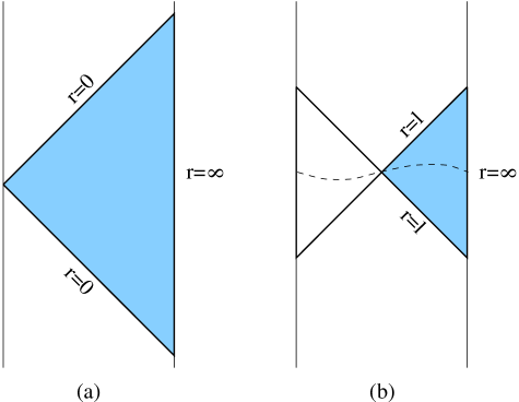
Figure 1: Regions of Anti-deSitter space covered by the parametrizations $k=+1,0,-1$ ($\mu=0$ in eq. (2)). With $k=+1$ all of AdS (the entire strip) is covered. (a) Portion covered in Poincaré (or horospheric) coordinates, $k=0$. (b) Portion covered by the hyperbolic slicing $k=-1$. Shown as a dashed line is a Cauchy surface.

The solution with $\mu=0$, $k=-1$, introduces a difference here. While isometric as well to AdS, it covers a smaller portion of the entire manifold, as the coordinate patch breaks down at $r=r_{+}=l$, see Fig. 1b. However, in contrast to the horizon in Poincaré coordinates, the horizon in this case is analogous to a Rindler horizon. There is an associated inverse temperature, $\beta=2\pi l$, and it has non–vanishing area. One should note that, among the $k=-1$ class of black hole solutions, the one that is isometric to AdS is not properly a black hole. It is completely non–singular, and in the absence of identifications it does not possess an event horizon. By contrast, the solutions with $\mu\neq 0$ possess a singularity at $r=0$.

For the $k=-1$ class of black holes, and in contrast to the $k=+1,0$ classes, the zero temperature solution is different from the one that is isometric to AdS. In fact, for $k=-1$ there is a range of negative values for $\mu$ such that the solutions still possess regular horizons. The minimum values of $\mu$ and $r_{+}$ that are compatible with cosmic censorship, for which the horizon is degenerate, are

$$\mu_{\rm ext}=-{2\over n-2}\left({n-2\over n}\right)^{n/2}l^{n-2}\ ,\qquad r_{\rm ext}=\sqrt{n-2\over n}l\ ,$$ (6)

and, in particular,

$$\mu_{\rm ext}=-{l^{2}\over 4}\ ,\qquad r_{\rm ext}={l\over\sqrt{2}},\qquad{\rm for\;}n=4\ .$$ (7)

For these values of the parameters, the black hole is extremal. The Penrose diagram for a hyperbolic black hole with negative $\mu$ is like that of a Reissner-Nordström-AdS black hole. For positive $\mu$ it is instead like that of a Schwarzschild-AdS black hole [12].

We now want to evaluate the thermodynamic functions for the solutions (1). In particular, if we have the quasilocal stress-energy tensor, which is defined on the boundary of a region of spacetime [15], as a function of the temperature then we can compute all other thermodynamic functions such as the energy or entropy. Recently, a prescription for computing the quasilocal stress tensor of a solution in AdS space has been proposed which appears to capture all of the information relevant to the dual field theory [16]. In this prescription, regularization does not proceed by the traditional subtraction of similar divergences from a reference state to which the solution is asymptotically matched. Instead, in the regularization proposed in [16] divergences are removed by subtraction of local counterterms at the boundary, in a manner closely analogous to the subtraction of divergences in field theory in curved spacetimes. As such, it appears to be particularly suitable for constructing the stress tensor of the dual CFT starting from a supergravity solution (see also [17]). This technique has been extended and generalized in [11] to all the dimensions of relevance for string/M-theory.

The metric on the boundary of AdS, $h_{\mu\nu}$ ($\mu,\nu=0,\dots,n-1$), is conformally related to the background metric of the field theory $\gamma_{\mu\nu}$. The conformal factor diverges near the boundary. By the AdS/CFT correspondence, the quasilocal stress tensor for AdS supergravity $\tau_{\mu\nu}$ can be translated into the expectation value of the stress tensor of the dual field theory $\langle T_{\mu\nu}\rangle$, in the strong coupling regime, as [17]

$$\langle{T_{\mu}}^{\nu}[\gamma_{\kappa\lambda}]\rangle=\left({h\over\gamma}\right)^{1/2}{\tau_{\mu}}^{\nu}[h_{\kappa\lambda}]\ ,$$ (8)

where the limiting approach to the boundary is assumed.

For the cases at hand the calculation of ${\tau_{\mu}}^{\nu}$ is straightforward. The appropriate conformal factor is $(h/\gamma)^{1/2}=(r/l)^{n}$ (see eq. (14) below) and we obtain

$$\langle{T_{\mu}}^{\nu}\rangle = {1\over 16\pi Gl}\left({2\epsilon^{0}_{k}\over n-1}+{\mu\over l^{n-2}}\right){\rm diag}(1-n,1,\dots,1)$$ (9)

$$= {1\over 16\pi Gl}\left({2\epsilon^{0}_{k}\over n-1}+{r_{+}^{n}\over l^{n}}+k{r_{+}^{n-2}\over l^{n-2}}\right){\rm diag}(1-n,1,\dots,1)\ ,$$

where (see [11])

$$\epsilon^{0}_{k}=(-k)^{n/2}{(n-1)!!^{2}\over n!}\qquad{\rm for\;even\;}n\ ,$$ (10)

and $\epsilon^{0}_{k}=0$ for odd $n$. It is worth noting that the form of this stress tensor is that of a thermal gas of massless radiation.

For the particular case of AdS₅ (and any $k$) it will be useful to note that the result can be written in a compact form as

$$\langle{T_{\mu}}^{\nu}\rangle={\pi\over 16Gl}\left({r_{+}\over\beta}\right)^{2}{\rm diag}(-3,1,1,1)\ .$$ (11)

The energy, given as a function of temperature through (5), can be read from (9) as

$$E_{BH}(\beta)={(n-1)V_{n-1}\over 16\pi Gl}\left({r_{+}^{n}\over l^{n}}+k{r_{+}^{n-2}\over l^{n-2}}+{2\epsilon^{0}_{k}\over n-1}\right)\ ,$$ (12)

with $V_{n-1}$ the volume of $d\Sigma^{2}_{k,n-1}$, i.e., the spatial volume of the field theory. With $E$ as a function of the temperature we can apply standard thermodynamic formulae to compute the entropy of the solution,

$$S_{BH}={V_{n-1}\over 4G}\left({r_{+}\over l}\right)^{n-1}\ ,$$ (13)

which satisfies, as expected, the Bekenstein–Hawking area law. We could equally well have computed the Euclidean action of the solutions and in this way obtain $\beta$ times the free energy $F$, from which the same values of $E$ and $S$ are recovered [11].

3 CFT duals of spherical and planar black holes—a brief review

The AdS/CFT correspondence states that the full non–perturbative dynamics of quantum gravity in a space that is asymptotic to AdS_n+1 can be formulated in terms of a dual conformal field theory defined on the $n$-dimensional causal boundary of the bulk spacetime. As discussed in detail in [11], the issue of what is the geometry of the boundary of a given solution is, to some extent, open, since it depends on how the spacetime is sliced radially as one approaches the boundary. As an example, it was explicitly shown in [11] how the boundary of (Euclidean) AdS_n+1 can be chosen to be $S^{n}$, ${\hbox{{\rm I}\kern-1.99997pt\hbox{\rm R}}}^{n}$, $H^{n}$, ${\hbox{{\rm I}\kern-1.99997pt\hbox{\rm R}}}\times S^{n-1}$, ${\hbox{{\rm I}\kern-1.99997pt\hbox{\rm R}}}\times H^{n-1}$, and several other geometries. We see then that the duals of AdS quantum gravity are in general conformal field theories defined on curved backgrounds with fixed geometry.

More specifically, in the coordinates chosen in (1), the metric at the boundary, as $r\rightarrow\infty$, is of the form

$$h_{\mu\nu}dx^{\mu}dx^{\nu}\rightarrow{r^{2}\over l^{2}}(-dt^{2}+d\Sigma^{2}_{k,n-1})\ .$$ (14)

The background spacetime for the dual field theory, $\gamma_{\mu\nu}$, is conformally related to this one, and the conformal factor can be chosen to cancel the divergent factor $r^{2}/l^{2}$ in (14), $\gamma_{\mu\nu}=\lim_{r\rightarrow\infty}{l^{2}\over r^{2}}h_{\mu\nu}$. In this way, the $k=+1,0,-1$ black holes admit a dual description in terms of a CFT on, respectively, ${\hbox{{\rm I}\kern-1.99997pt\hbox{\rm R}}}\times S^{n-1}$, ${\hbox{{\rm I}\kern-1.99997pt\hbox{\rm R}}}^{n}$, ${\hbox{{\rm I}\kern-1.99997pt\hbox{\rm R}}}\times H^{n-1}$, each of these otherwise known as the Einstein universe, Minkowski spacetime, and the static open universe, respectively. However, it should be clear as well that by slicing, say, the $k=\pm 1$ solutions in an adequate way, the spherical and hyperbolic black holes can be described as states of the field theory on Minkowski space. This can be achieved more simply by choosing adequately the conformal factor between $h_{\mu\nu}$ and $\gamma_{\mu\nu}$, see [18] for an example. We will make use of this idea later in section 5.

The case of $k=0$ is particularly simple since, in the absence of any scale other than the thermal wavelength, conformal invariance, together with staticity and homogeneity of the space, determines the stress tensor of the CFT to take the form

$$\langle{T_{\mu}}^{\nu}\rangle_{CFT}={\sigma_{sb}\over\beta^{n}}{\rm diag}\left(-1,{1\over n-1},\dots,{1\over n-1}\right)\ .$$ (15)

The energy and entropy follow as

$$E_{CFT}=\sigma_{sb}V_{n-1}\beta^{-n},\qquad S_{CFT}={n\over n-1}\sigma_{sb}V_{n-1}\beta^{-n+1}\ .$$ (16)

The factor $\sigma_{sb}$ is the Stefan-Boltzmann constant, which is determined by the precise field content of the CFT, and grows with the number of degrees of freedom of the theory. We will give it below for the cases of interest.

As observed in [5, 3], for planar ($k=0$) black holes $r_{+}\sim\beta^{-1}$, so the CFT thermodynamic functions (15), (16), agree with their AdS black hole counterparts (9), (12), (13) up to the Stefan-Boltzmann factors (notice that for $k=0$, $\epsilon^{0}_{k}=0$). If one wants to make this equivalence more precise and try to compare the precise Stefan-Boltzmann factors, then a specific dual field theory has to be supplied. String/M-theory provides duals for AdS_n+1, $n=2,3,4,6,$ as the CFTs describing the world–volume dynamics of stacks of parallel (D1$+$D5)-, M2-, D3-, M5-branes. The dictionary for translating AdS/CFT quantities reads

$$c={3l\over 2G}\quad{\rm for\;AdS}_{3}\ , \quad N^{3/2}={3\over 2\sqrt{2}}{l^{2}\over G}\quad{\rm for\;AdS}_{4}\ ,$$

$$N^{2}={\pi l^{3}\over 2G}\quad{\rm for\;AdS}_{5}\ , \quad N^{3}={3\pi^{2}\over 16}{l^{5}\over G}\quad{\rm for\;AdS}_{7}\ ,$$ (17)

where $N$ is the number of parallel branes. The powers of $N$ displayed above are measures of the number of “unconfined” degrees of freedom: for AdS₅, $N$ is the rank of the gauge group of the dual ${\cal N}{=}4$ supersymmetric four dimensional $SU(N)$ Yang–Mills theory. For AdS₃, $c$ is the central charge of the dual CFT in two dimensions; however, since there are no $k=-1$ black holes in AdS₃ we will not deal with this case any longer. Note that for generic number of dimensions, the entry in the dictionary can be expected to be

$$N^{n/2}\approx{l^{n-1}\over G}\quad{\rm for\;AdS}_{n+1}\ .$$ (18)

Let us focus now on the pair AdS₅/(${\cal N}{=}4$ SYM), in a discussion which can be traced back to [4]. Using (17), the results from (12) and (13) for $k=0$, $n=4$, become

$$E_{BH}={3\pi^{2}N^{2}\over 8\beta^{4}}V_{3}\ ,\quad S_{BH}={\pi^{2}N^{2}\over 2\beta^{3}}V_{3}\ .$$ (19)

On the other hand, it is a standard result from free field theory at finite temperature that the factor $\sigma_{sb}$ in four dimensional thermal Minkowski space for fields of different spin is

$$\sigma_{sb}={\pi^{2}\over 30}\left(n_{0}+{7\over 4}n_{1/2}+2n_{1}\right)\ ,$$ (20)

where $n_{0}$ is the number of (real) scalars, $n_{1/2}$ is the number of Weyl (or Majorana) fermions, and $n_{1}$ the number of gauge vectors. For ${\cal N}{=}4$ $SU(N)$ SYM at large $N$,

$$n_{0}=6N^{2}\ ,\qquad n_{1/2}=4N^{2}\ ,\qquad n_{0}=N^{2}\ .$$ (21)

By plugging these values into (20) we find $\sigma_{sb}=\pi^{2}N^{2}/2$, which leads to the well–known result [4] that

$$E_{BH}={3\over 4}E_{SYM}\ ,\quad S_{BH}={3\over 4}S_{SYM}\ .$$ (22)

The SYM result is obtained by computing one–loop vacuum diagrams, i.e., it is the leading term in a perturbative expansion in the ’t Hooft parameter $g_{YM}^{2}N$. By contrast, the supergravity approximation, on which the AdS black hole result is based, is reliable only for large $g_{YM}^{2}N$. The mismatch in (22) is therefore interpreted as a strong coupling effect. An argument for why the entropy should change only by a numerical factor of order one has been given in [19].

Let us comment on two aspects of (22). The first one is that the values for the energy and entropy at strong coupling are smaller than their perturbative values. As a matter of fact, as noted in [4], the result for $E_{BH}$ would agree with a perturbative calculation if, for some reason, at strong coupling we had effectively $n_{0}=6N^{2}$, $n_{1/2}=3N^{2}$, $n_{0}=0$, i.e., if only the scalar multiplets contributed to the free energy, whereas the fields in the (${\cal N}{=}1$) vector multiplet could not be excited. There is therefore a reduction in the effective number of degrees of freedom at strong coupling. The second aspect we want to emphasize, for reasons which will be better appreciated later, is that both the energy and the entropy are reduced by the same factor $3/4$. That this should happen is a consequence of the fact that the temperature dependence $E\sim\beta^{-4}$ is the same at both strong and weak coupling, since it is fixed by conformal invariance. Therefore, even if some degrees of freedom may get frozen at strong coupling, it appears that all the states that contribute to the entropy also make a contribution to the energy of the system.

For the cases of AdS₄ and AdS₇, the dual conformal field theories of $N$ parallel M2- and M5-branes are poorly known, and as a consequence it is impossible at present to discuss these cases in the same detail as the AdS₅/SYM pair.

Overall, we can say that the qualitative aspects of the AdS/CFT duality for planar black holes are fairly well understood, and in particular for AdS₅ the free field theory seems to capture a good deal of the thermodynamics at strong coupling.

Turn now to $k=1$, i.e., spherical black holes and their dual CFTs, which according to (14) are naturally defined on spatial spheres $S^{n-1}$. This introduces a length scale $l$ in the theory. As it happens, in this instance there appears a phenomenon that is absent from planar (and hyperbolic) AdS black holes. The thermodynamic analysis of the black hole solutions reveals a phase transition at finite temperature between the state corresponding to $\mu=0$ (global AdS) and the (large) black hole phase [7, 3, 6]. The low temperature phase (global AdS) is interpreted as a “confined” phase [3, 6]. This phenomenon, although expected from generic considerations, can not be seen from a perturbative analysis of the field theory. Therefore, even if results for conformal fields on $S^{1}\times S^{n-1}$ at a perturbative level (free field theory) are available [20], which can be employed to compute $E_{CFT}(\beta)$, they can not be expected to provide us with any information about the strongly coupled regime, at least at low temperatures: the phase transition throws us into a region where perturbative field theory is useless.

Nevertheless, there is one result that can be meaningfully compared, namely, the Casimir energy associated to the field theory on ${\hbox{{\rm I}\kern-1.99997pt\hbox{\rm R}}}\times S^{3}$. The dual supergravity solution is AdS₅ in global coordinates, which is protected from strong coupling (string $\alpha^{\prime}$) corrections [21]. Moreover, the Casimir energy is essentially determined by the central charges of the ${\cal N}=4$ SYM theory, which receive no higher loop corrections [22]. Indeed, it has been proven that the result from free field theory matches precisely the AdS calculation [16].

4 AdS/CFT duality for hyperbolic black holes

Hyperbolic black holes share with planar black holes the property that they do not exhibit phase transitions at finite temperature. At any temperature the phase structure is dominated by a black hole. Then, the dual field theory at strong coupling is expected to remain in an unconfined phase [8, 9]. Therefore, even if interactions are expected to introduce modifications (as was the factor $3/4$ in (22) for planar black holes), we can hope to be able to extract valuable information by trying to connect the weakly coupled and strongly coupled regimes.

An important feature of hyperbolic black holes is that the curvature of the hyperbolic space $H^{n-1}$ introduces a new scale into the field theory, and as a result the temperature dependence is not fully fixed by conformal invariance. The case of flat space is contained in this class of black holes as a limit (as was also for spherical black holes), which can be characterized as the high temperature limit. At any other temperatures the thermodynamic functions are more complicated, and encode more information than in the case of flat spacetime. In particular, the relationship between energy and entropy is not as simple as in (16), and the thermodynamic magnitudes become more sensitive to the field theory content.

Furthermore, we will be able to crucially exploit a novel feature, absent from the other two classes of black holes. As mentioned above, there is one particular state, the one corresponding to $\mu=0$ (i.e., $r_{+}=l$, $\beta=2\pi l$), which is isometric to AdS. Since AdS₅($\times S^{5}$) is an exact string state, protected from corrections in the ‘tHooft coupling $g^{2}_{YM}N$, results at perturbative level can be extrapolated to strong coupling. When we write AdS with the hyperbolic slicing the situation is, however, interestingly non–trivial, since the $k=-1$ description of AdS does not cover all of the spacetime, rather only a wedge. Accordingly, in a computation of, say, the partition function of the theory, states that lie outside this wedge are traced out, and will give rise to an entropy, sometimes called “entanglement entropy” [23]. More precisely, on a Cauchy surface in the $k=-1$ patch, such as shown Fig. 1b, the data to the left of the Einstein-Rosen bridge are traced out. On the supergravity side, this entropy appears as an entropy associated to the acceleration horizon. On the field theory side we can compute the entropy of states on a hyperbolic space. The detailed comparison of these quantities will only be possible for AdS₅/SYM, so we will devote most of the section to this case. Other sides of the relation to acceleration horizons will appear in section 5.

4.1 AdS₅/SYM on a hyperboloid

Let us then start by translating the strong coupling, black hole results of section 2 into field theory language by using (17), focusing on the AdS₅/SYM dual pair. From eqs. (11), (5) we find, for the stress-energy tensor of strongly coupled SYM on hyperbolic space at finite temperature

$$\langle{T_{\mu}}^{\nu}\rangle_{\rm(sugra)}={\pi^{2}N^{2}\over 32\beta^{4}}\left(1+\sqrt{1+{2\beta^{2}\over\pi^{2}l^{2}}}\right)^{2}{\rm diag}(-3,1,1,1)\ .$$ (23)

In this geometry, the energy is equal to $E=-\int d^{3}x\langle{T_{0}}^{0}\rangle$. On the other hand, from (13), the entropy is

$$S_{\rm(sugra)}={\pi^{2}N^{2}V_{3}\over 16\beta^{3}}\left(1+\sqrt{1+{2\beta^{2}\over\pi^{2}l^{2}}}\right)^{3}\ .$$ (24)

It is straightforward to see that in the high temperature limit $\beta\rightarrow 0$ we recover the results for flat space (19).

As explained, there are two states of particular interest. One is the extremal, zero temperature ($\beta\rightarrow\infty$) black hole (7), and the other is the solution isometric to AdS ($\beta=2\pi l$). For the first one we find

$$E_{\rm(sugra)}|_{\beta\rightarrow\infty}=0$$ (25)

and

$$S_{\rm(sugra)}|_{\beta\rightarrow\infty}={N^{2}\over 2^{5/2}\pi l^{3}}V_{3}\ .$$ (26)

Notice that the energy for this state, and actually the entire stress tensor, is zero, so it seems appropriate to identify it with the ground state of the theory. Nevertheless, its entropy does not vanish, a surprising fact that was noted in [11] and which we will discuss below.

For AdS₅ in the hyperbolic slicing, i.e., the state at $\beta=2\pi l$,

$$E_{\rm(sugra)}|_{\beta=2\pi l}={3N^{2}\over 32\pi^{2}l^{4}}V_{3}\ ,$$ (27)

and

$$S_{\rm(sugra)}|_{\beta=2\pi l}={N^{2}\over 2\pi l^{3}}V_{3}\ .$$ (28)

Turning now to the weakly coupled regime, we will make use of results obtained in [24] for the stress tensor of conformal fields in $S^{1}\times H^{3}$. The essential input in the computation is the density of eigenvalues of the wave operator in $H^{3}$ for fields of different spins. If $h(s)$ is the number of helicities of the spin $s$ field, and $n_{s}$ is the number of such fields, then, for $s=0,1/2,1$, one gets

$$\langle{T_{\mu}}^{\nu}\rangle_{\rm(gauge)}=\sum_{s}{n_{s}h(s)\over 6\pi^{2}l^{4}}\int_{0}^{\infty}d\lambda{\lambda(\lambda^{2}+s^{2})\over e^{\beta\lambda/l}-(-1)^{2s}}\;{\rm diag}(-3,1,1,1)\ .$$ (29)

The integrals can be performed explicitly, and with $h(0)=1$, $h(1/2)=h(1)=2$ we find

$$\langle{T_{\mu}}^{\nu}\rangle_{\rm(gauge)}={\pi^{2}\over 90\beta^{4}}\left(n_{0}+{7\over 4}n_{1/2}+2n_{1}+{5\beta^{2}\over 8\pi^{2}l^{2}}(n_{1/2}+8n_{1})\right){\rm diag}(-3,1,1,1)\ .$$ (30)

Having the energy $E(\beta)$, the entropy can be computed by using the first law of thermodynamics, with the result

$$S_{\rm(gauge)}={2\pi^{2}V_{3}\over 45\beta^{3}}\left(n_{0}+{7\over 4}n_{1/2}+2n_{1}+{15\beta^{2}\over 16\pi^{2}l^{2}}(n_{1/2}+8n_{1})\right)\ .$$ (31)

In the high temperature limit $\beta\rightarrow 0$ the results from the previous section for flat spacetime are recovered. However, attention should be drawn to the mixing of temperature dependences in (30) and (31). In contrast to the simple flat space dependence (16), which would still hold if only scalar fields were present, the presence of higher spin fields introduces a sensitivity to the curvature of the space. This is reflected in the $\beta^{2}$ term inside brackets, which has a different factor in (30) and (31).

We specialize now to the field content of large $N$ $SU(N)$ ${\cal N}{=}4$ Super Yang–Mills theory, (21), to find

$$\langle{T_{\mu}}^{\nu}\rangle_{\rm(gauge)}={\pi^{2}N^{2}\over 6\beta^{4}}\left(1+{\beta^{2}\over 2\pi^{2}l^{2}}\right){\rm diag}(-3,1,1,1)\ ,$$ (32)

$$S_{\rm(gauge)}={2\pi^{2}N^{2}\over 3\beta^{3}}V_{3}\left(1+{3\beta^{2}\over 4\pi^{2}l^{2}}\right)\ .$$ (33)

Compare now these results with the ones in the strongly coupled regime, eqs. (23), (24). It is apparent that the dependence on the temperature is rather different, and in fact both come to agree only at high temperatures, where we recover the same relationship as in (22).

For the ground state at zero temperature, the results

$$E_{\rm(gauge)}|_{\beta\rightarrow\infty}=S_{\rm(gauge)}|_{\beta\rightarrow\infty}=0$$ (34)

are as expected for a conventional ground state. On the other hand, for the state at $\beta=2\pi l$ we get

$$E_{\rm(gauge)}|_{\beta=2\pi l}={3N^{2}\over 32\pi^{2}l^{4}}V_{3}\ ,$$ (35)

$$S_{\rm(gauge)}|_{\beta=2\pi l}={N^{2}\over 3\pi l^{3}}V_{3}\ .$$ (36)

It is immediate to notice that for both the ground state and the state at $\beta=2\pi l$ the energy computed using free field theory agrees with the results in the strong coupling (supergravity) regime, eqs. (27), (25).

As a matter of fact, not only in supergravity but also in the field theory on $S^{1}\times H^{n-1}$ the state at $\beta=2\pi l$ is singled out among states at other temperatures: it can be formally obtained from the vacuum of the Einstein universe ${\hbox{{\rm I}\kern-1.99997pt\hbox{\rm R}}}\times S^{n-1}$ by “thermalization at imaginary temperature” $T=(2\pi il)^{-1}$ [24]. The two calculations of (a) the Casimir energy on ${\hbox{{\rm I}\kern-1.99997pt\hbox{\rm R}}}\times S^{3}$ [16], and (b) the energy of the state at $\beta=2\pi l$ on $S^{1}\times H^{3}$, eqs. (35) and (27), are in this light seen as the result of formally equivalent calculations. This is reflected in the fact that both follow from the same central charge of the field theory.

Despite the agreement for the energies of these states, the results for the entropy obtained from supergravity are both different from the one–loop field theory results. Eq. (26) is telling us that at infinite ‘tHooft coupling there is a large degeneracy for the state at zero temperature and zero energy density. Such ground state degeneracies are highly unusual. The mismatch in the entropy for the state at $\beta=2\pi l$ is not less unexpected. As we had remarked, this state is described in the bulk of AdS as a wedge of the full AdS₅ spacetime. We shall argue in sec. 6 that not only the energy, but also the entropy of this state would have been expected to be protected from corrections in the coupling. Nevertheless, we find at strong coupling an entropy larger than that obtained from field theory at the lowest perturbative order. The relationship between both is simple,

$$S_{\rm(sugra)}|_{\beta=2\pi l}={3\over 2}S_{\rm(gauge)}|_{\beta=2\pi l}\ .$$ (37)

This is in stark contrast to the situation for planar black holes, where there is an effective reduction at strong coupling in the number of states available to the gauge theory. Here we find instead an enhancement, but one that affects only the entropy, not the energy.

It can be readily checked that the values of the energy at weak and strong coupling agree only for the two values of the temperature $\beta=2\pi l,\;\infty$. Indeed, we would not have expected agreement at any other temperature, due to strong coupling corrections. It is therefore difficult to meaningfully make comparisons of the entropy expected at different temperatures. Notice, however, that, at any temperature,

$${S_{\rm(gauge)}(\beta)\over E_{\rm(gauge)}(\beta)}\leq{S_{\rm(sugra)}(\beta)\over E_{\rm(sugra)}(\beta)}\ ,$$ (38)

with equality only at infinite temperature. Although the different temperature dependence of different fields makes it difficult to take this too literally, this inequality would suggest that at strong coupling there appear to be more states contributing to the entropy than those that contribute to the energy.

One last magnitude which is interesting for comparison purposes is the specific heat, since it measures the response (susceptibility) of the degrees of freedom to thermal excitation. We find

$$C_{\rm(sugra)}={3\pi^{2}N^{2}\over 16\beta^{3}}{\left(1+\sqrt{1+{2\beta^{2}\over\pi^{2}l^{2}}}\right)^{3}\over\sqrt{1+{2\beta^{2}\over\pi^{2}l^{2}}}}\ ,$$ (39)

$$C_{\rm(gauge)} = {2\pi^{2}\over 15\beta^{3}}\left(n_{0}+{7\over 4}n_{1/2}+2n_{1}+{5\beta^{2}\over 16\pi^{2}l^{2}}(n_{1/2}+8n_{1})\right)$$ (40)

$$= {2\pi^{2}N^{2}\over\beta^{3}}\left(1+{\beta^{2}\over 4\pi^{2}l^{2}}\right)\ .$$

For the different temperatures of interest these become

$$C_{\rm(gauge)}|_{\beta\rightarrow\infty}\rightarrow{4\over 3}C_{\rm(sugra)}|_{\beta\rightarrow\infty}\rightarrow{N^{2}\over 2l^{2}\beta}\ ,$$ (41)

$$C_{\rm(gauge)}|_{\beta=2\pi l}=C_{\rm(sugra)}|_{\beta=2\pi l}={N^{2}\over 2\pi l^{3}}\ ,$$ (42)

while at high temperature we recover the flat space result

$$C_{\rm(gauge)}|_{\beta\rightarrow 0}\rightarrow{4\over 3}C_{\rm(sugra)}|_{\beta\rightarrow 0}\rightarrow{2\pi^{2}N^{2}\over\beta^{3}}\ ,$$ (43)

in which the specific heat grows with the characteristic four-dimensional dependence $\sim\beta^{-3}=T^{3}$.

At low temperatures it is the spin-1/2 and spin-1 fields which dominate the specific heat, at least at weak coupling (see (40)). The curvature of $H^{3}$, to which these fields are sensitive, makes them more susceptible of being excited and as a consequence the specific heat grows faster, as $C\sim T$ instead of $T^{3}$. Remarkably, this is also the behavior we find at strong coupling, where we do not know how to separate the contributions from different sets of degrees of freedom. This suggests that, at low temperatures, the degrees of freedom at strong coupling are not too dissimilar in nature from those that operate at weak coupling. Curiously, the precise numerical factor is off by the same fraction ${4/3}$ as at high temperatures.

Finally, at $\beta=2\pi l$ the specific heats are exactly the same in the strongly coupled and weakly coupled regimes. It would appear that even if extra states are present which contribute to the entropy (albeit not to the energy), the susceptibility to thermal excitation is still dominated by those states that make up the energy density.

4.2 Other dimensions

The results (12) and (13) for the energy and entropy of topological black holes in section 2 can be expressed in terms of the temperature using (5) and then converted into expressions for field theory at strong coupling using the dictionary (17) or, more generally, (18). In turn, it is possible as well to compute the corresponding quantities for free fields on hyperbolic space at finite temperature. The contribution from a spin $s$ field to the energy on $S^{1}\times H^{n-1}$ is obtained as

$$E_{s}(\beta)=h(s){V_{n-1}\over\omega_{n-1}l^{n}}\int_{0}^{\infty}d\lambda{\lambda\mu_{s}(\lambda)\over e^{\beta\lambda/l}\mp 1}\ ,$$ (44)

where $h(s)$ is, as before, the number of physical states (helicities) for each field, $\omega_{n-1}$ is the volume of the unit $(n-1)$-sphere, the $-$ ($+$) sign in the denominator applies to boson (fermion) fields, and $\mu_{s}(\lambda)$ measures the degeneracy (density) of eigenvalues of the wave operator on the hyperbolic space. It is known in the mathematical literature as the Plancherel measure. The latter has been computed for hyperbolic spaces in arbitrary dimensions for a wide variety of fields. To quote, for $H^{N}$, for real scalars [25],

$$\mu_{sc}(\lambda)={\pi\over[2^{N-2}\Gamma(N/2)]^{2}}\left|{\Gamma(i\lambda+{N-1\over 2})\over\Gamma(i\lambda)}\right|^{2}\ .$$ (45)

For spinors [26],

$$\mu_{sp}(\lambda)={\cosh\pi\lambda\over[2^{N-2}\Gamma(N/2)]^{2}}\left|\Gamma\left(i\lambda+{N\over 2}\right)\right|^{2}\ .$$ (46)

For (co-exact) $p$-forms, $h(s)={(N-1)!\over p!(N-p-1)!}$ (which must be halved for self-dual forms), and [27]

$$\mu_{p-{\rm form}}(\lambda)={\pi\over[2^{N-2}\Gamma(N/2)]^{2}}{1\over\lambda^{2}+({N-1\over 2}-p)^{2}}\left|{\Gamma(i\lambda+{N+1\over 2})\over\Gamma(i\lambda)}\right|^{2}\ ,$$ (47)

(this contains the scalar case for the value $p=0$, and gauge vectors for $p=1$).

Using these results, we can compute for the free field content of a single M2-brane, i.e., an ${\cal N}=8$ supermultiplet in $d=3$,

$$E_{M2}(\beta)={V_{2}\over 4l^{3}}\int_{0}^{\infty}d\lambda\;\lambda^{2}\left({n_{0}\tanh\pi\lambda\over e^{\beta\lambda/l}-1}+{n_{1/2}\coth\pi\lambda\over e^{\beta\lambda/l}+1}\right)\ ,$$ (48)

with $n_{0}=8$ and $n_{1/2}=8$. It is not possible to give the results of the integrations in closed form for arbitrary values of $\beta$, although they simplify for $\beta=2\pi l$. However, it is easy to see that these results bear little resemblance to the ones that follow from supergravity calculations. Indeed, from (48) one easily sees that

$$E_{M2}|_{\beta\rightarrow\infty}=S_{M2}|_{\beta\rightarrow\infty}=0\ ,$$ (49)

whereas the strong coupling calculation would yield

$$E_{M2(\rm strong)}|_{\beta\rightarrow\infty}=-{N^{3/2}V_{2}\over 9\sqrt{6}\pi l^{3}}\ ,\quad S_{M2(\rm strong)}|_{\beta\rightarrow\infty}={N^{3/2}V_{2}\over 9\sqrt{2}l^{2}}\ .$$ (50)

Notice that not only the entropy but also the energy of this state is different from zero. Indeed, as noted in [11], for AdS₄ (and in fact for all even $d$ AdS_d) it is the state at $\beta=2\pi l$ that has zero energy. And nevertheless it has non–zero entropy.

These results for AdS₄ are even more striking than those for AdS₅: the state that is isometric to AdS₄ is a state at finite temperature and with non–zero entropy, which nevertheless has zero energy density! This looks markedly different from conventional field theory. Moreover, there appear states, namely, those for $\mu_{e}\leq\mu<0$, with total negative energy. The meaning of these is unclear.

For the free field content of the $(2,0)$ superconformal theory on a single M5-brane (i.e., the $d=6$ tensor supermultiplet),

$$E_{M5}(\beta) = {V_{5}\over 36\pi^{3}l^{6}}\int_{0}^{\infty}d\lambda\;\lambda\left({5\lambda^{2}(\lambda^{2}+1)\over e^{\beta\lambda/l}-1}+{8(\lambda^{2}+1/4)(\lambda^{2}+9/4)\over e^{\beta\lambda/l}+1}+{3(\lambda^{2}+1)(\lambda^{2}+2)\over e^{\beta\lambda/l}-1}\right)$$ (51)

$$= {V_{5}\pi^{3}\over 1440\beta^{6}}\left(80+84{\beta^{2}\over\pi^{2}l^{2}}+55{\beta^{4}\over\pi^{4}l^{4}}\right)\ .$$

This free field theory expression has nothing exotic about it. As the temperature goes to zero, the energy vanishes. So does the entropy, too, as can be checked easily. However, the results at strong coupling from AdS calculations are puzzling: neither the state at zero temperature nor the one at $\beta=2\pi l$ have zero energy. Both, moreover, have non–zero entropy.

It appears quite likely that in all these cases exotic states that contribute to the entropy but not to the energy would be required to account for the black hole entropy. However, and in contrast to the case of AdS₅/SYM, for AdS₄ and AdS₇ free field theory yields little useful information.

5 Dual CFT description in Rindler space

In the previous section we have chosen to describe hyperbolic black holes in terms of the theory on ${\hbox{{\rm I}\kern-1.99997pt\hbox{\rm R}}}\times H^{n-1}$. However, as noted at the beginning of section 3, it is possible to perform the entire description in terms of the theory on flat space. All one has to do is slice the AdS black hole spacetime in a way that, near the boundary, the constant radius sections are flat. Let us start by showing how this can be done explicitly for the solutions which are locally isometric to AdS_n+1. In Poincaré coordinates,

$$ds^{2}={r^{2}\over l^{2}}(-du\;dv+dx_{i}^{2})+{l^{2}\over r^{2}}dr^{2}$$ (52)

($i=1,\dots,n-2$), where $u,v$ are light-cone coordinates $u=t-x_{n-1}$, $v=t+x_{n-1}$. Now change

$$u=-\zeta\sqrt{1-{l^{2}\over{\tilde{r}}^{2}}}\;e^{-\eta/l}\ ,\quad v=\zeta\sqrt{1-{l^{2}\over{\tilde{r}}^{2}}}\;e^{\eta/l}\ ,$$ (53)

$$r=l{{\tilde{r}}\over\zeta}\ ,$$ (54)

leaving $x_{i}$ unchanged, to find AdS in hyperbolic ($k=-1$) coordinates

$$ds^{2}=-\left({{\tilde{r}}^{2}\over l^{2}}-1\right)d\eta^{2}+{d{\tilde{r}}^{2}\over{{\tilde{r}}^{2}\over l^{2}}-1}+{\tilde{r}}^{2}{d\zeta^{2}+dx_{i}^{2}\over\zeta^{2}}$$ (55)

(the spatial hyperboloid $H^{n-1}$ is parametrized here in horospheric coordinates). The Killing horizon at ${\tilde{r}}=l$ is mapped onto the null surfaces $u,v=0$. Now notice that as the boundary is approached ($r,{\tilde{r}}\rightarrow\infty$) the transformation (53) between boundary coordinates becomes

$$u\rightarrow-\zeta e^{-\eta/l}\ ,\quad v\rightarrow\zeta e^{\eta/l}\ .$$ (56)

This is precisely the transformation between Minkowski and Rindler coordinates. Indeed, as we approach the boundary,

$${r^{2}\over l^{2}}(-du\;dv+dx_{i}^{2}) \rightarrow {{\tilde{r}}^{2}\over l^{2}}\left(-d\eta^{2}+l^{2}{d\zeta^{2}+dx_{i}^{2}\over\zeta^{2}}\right)$$ (57)

$$= {r^{2}\over l^{2}}\left(-\zeta^{2}\left({d\eta\over l}\right)^{2}+d\zeta^{2}+dx_{i}^{2}\right)={r^{2}\over l^{2}}ds^{2}_{R}\ ,$$

where $ds^{2}_{R}$ is the metric on Rindler space (with time rescaled by $l$). The conformal factor that effects the change between ${\hbox{{\rm I}\kern-1.99997pt\hbox{\rm R}}}\times H^{n-1}$ and the flat (Rindler) space at the asymptotic boundary is $r^{2}/{\tilde{r}}^{2}=l^{2}/\zeta^{2}$.

Therefore AdS in hyperbolic coordinates corresponds, in the description in terms of a field theory in flat space, to the Rindler state of the CFT at $\beta=2\pi l$. This is, of course, the Rindler description of the Minkowski vacuum. For the Rindler observer, the latter is a mixed thermal state described by a density matrix.

This relationship between the solutions that are isometric to AdS, and their corresponding states in the dual field theories, is entirely analogous to that existing between BTZ black holes and AdS₃ and the corresponding states in the dual $1+1$ CFTs [29], except for the fact that we have not performed discrete identifications.

For black holes with $\mu\neq 0$ it is not simple to find a global coordinate transformation that effects the change from the hyperbolic to the flat space description. However, we only need the conformal factor that transforms the boundary geometries near infinity, and then use it to transform the stress tensors as in eq. (8). This was the procedure followed in [18] to find a description of spherical black holes in terms of the SYM theory in Minkowski space. We can do the same thing here using the conformal factor $l^{2}/\zeta^{2}$, which according to eq. (57) takes us to a Rindler space geometry at the boundary.

We conclude then that, in the dual field theory on flat space, hyperbolic black holes correspond to thermal Rindler states at temperature $\beta$. The one at temperature $\beta=2\pi l$ is singled out as corresponding to the Poincaré invariant vacuum in Minkowski space. Other states are described, in imaginary time, using geometries with a conical singularity at $\zeta=0$. Notice, however, that there is no conical singularity in the description on ${\hbox{{\rm I}\kern-1.99997pt\hbox{\rm R}}}\times H^{n-1}$.

Given the conformal factor between hyperbolic space and Rindler space, the stress tensor in the latter is constructed as

$${\langle{T_{\mu}}^{\nu}\rangle}^{\rm(Rindler)}(\beta)={l^{4}\over\zeta^{4}}\left[{\langle{T_{\mu}}^{\nu}\rangle}^{\rm(Hyper)}(\beta)-{\langle{T_{\mu}}^{\nu}\rangle}^{\rm(Hyper)}(\beta=2\pi l)\right]$$ (58)

(we are implicitly using the fact that the trace anomaly vanishes for both spaces). As a matter of fact, the simple conformal relationship between Rindler and hyperbolic space has been put to use before in order to solve one of them from knowledge of the other [24] (see also, e.g., [30, 31] and references therein). Conventionally, we have subtracted a $\beta$-independent tensor term in (58) in order that that the stress tensor vanishes at $\beta=2\pi l$. The reason is that $\langle T_{\mu\nu}\rangle$ being a tensor that vanishes in the Minkowski vacuum, it should vanish in that state in any other coordinate system. Recall that the Minkowski vacuum is the global state of minimum energy, which realizes the full Poincaré symmetry of the theory. The Rindler vacuum (the state for $\beta\rightarrow\infty$) can have lower energy because the minimization of the energy in Rindler space is constrained only by a subgroup of the Poincaré symmetries. The divergence of the vacuum energy density as $\zeta\rightarrow 0$ is only expected, since the vacuum is made to accelerate infinitely hard at that point.

The construction (58) works the same way at weak and strong coupling. Since at $\beta=2\pi l$ the stress tensor ${\langle{T_{\mu}}^{\nu}\rangle}^{\rm(Hyper)}$ is the same in both regimes, the negative energy of the Rindler vacuum is the same at zero and infinite coupling. Moreover, the subtraction of such a quantity does not affect the calculation of the entropy. Therefore, the subtraction in (58) does not introduce any significant modification in our discussion.

The entropy density $s$ in Rindler space is equally obtained by rescaling the one in hyperbolic space as

$$s^{\rm(Rindler)}(\beta)={l^{3}\over\zeta^{3}}s^{\rm(Hyper)}(\beta)\ .$$ (59)

Notice that the finite entropy density of the Minkowski vacuum is not to be subtracted, since it is physically relevant as entanglement entropy. A Minkowski (global) observer assigns zero entropy to this state. An accelerating observer, however, detects quantum fluctuations of the vacuum (they appear to him as thermal fluctuations) and is sensitive to the vacuum activity of the global fundamental state. The Rindler entropy density at $\beta=2\pi l$ therefore yields a measure of the states that are subject to quantum fluctuations in the global vacuum.

The discussion of the previous section can now be couched in terms of statements about the energy and entropy of the CFT in Rindler space. We therefore find that the Rindler vacuum is, at infinite coupling, highly degenerate. On the other hand, a Rindler observer accelerating in the Minkowski vacuum measures an entropy density for SYM larger than would have been expected from the weak coupling calculation.

6 Finite ’t Hooft coupling corrections

The calculations we have presented so far have been performed at two opposite ends of the scale of the SYM ’t Hooft coupling, $g^{2}_{YM}N$. Gauge theory computations have been performed at the level of one–loop vacuum diagrams, i.e., $g^{2}_{YM}N=0$, whereas the supergravity approximation to type IIB string theory is reliable when $g^{2}_{YM}N=l^{4}/(2\alpha^{\prime 2})\rightarrow\infty$. In this section we want to discuss the corrections that arise when $g^{2}_{YM}N$ deviates from these limits. The study will be carried out only for the case of AdS₅/SYM.

Conformal invariance imposes strong restrictions on the form of finite coupling corrections for the planar case, $k=0$. The temperature dependence is fixed, so a thermodynamic function like the free energy must be of the form

$$F=F_{0}\;f(g^{2}_{YM}N)\ ,$$ (60)

where $F_{0}$ is the value at zero coupling. It is clear that the energy and entropy are corrected by the same function $f(g^{2}_{YM}N)$. In contrast, for the hyperbolic or spherical systems one will typically have

$$F=F_{0}\;f(g^{2}_{YM}N,\beta/l)\ ,$$ (61)

and the temperature dependence will change in general. Indeed, we have seen explicitly that the supergravity and gauge theory expressions for the energy and entropy in the hyperbolic case have a very different dependence on $\beta$. One would ascribe the differences to the effect of interactions as the coupling is turned on.

Perturbative interactions will change the weak coupling result through higher–loop diagrams. For the SYM theory in Minkowski space, these have been computed in [32]. However, the extension of these calculations to the spherical or hyperbolic cases is much more difficult, since it implies solving an interacting theory in a curved background.

At the other end of the scale, large $g^{2}_{YM}N$, the first corrections arise from $O(\alpha^{\prime 3})=O((g^{2}_{YM}N)^{-3/2})$ corrections to the effective IIB superstring action at low energies. The relevant term in the Euclidean action is [33, 34]

$$\delta I=-{1\over 16\pi G_{10}}\int d^{10}x\sqrt{g^{(10)}}\alpha^{\prime 3}{\zeta(3)\over 8}W\ ,$$ (62)

where $W$ is a scalar constructed out of contractions of four Weyl tensors. Using this term, finite coupling corrections to the thermodynamics of planar black holes have been studied in [34, 35], and spherical black holes in [36, 37]. The study of the latter has been taken further in [38], where the corrections to hyperbolic black holes have been calculated as well.

In principle, one must consider corrections in the entire ten dimensional theory, since it is not possible to keep the size of the sphere $S^{5}$ fixed [35]. However, on reduction to five dimensions it is easy to see that neither the dilaton nor the scale factor of the sphere will contribute on–shell to the effective five–dimensional action for as long as they fall off fast enough at asymptotic infinity. It is therefore possible to compute the Euclidean action of the corrected solutions in a five dimensional formulation for solutions asymptotic to AdS₅ [34]. This will be important for us, since it will permit us to employ the intrinsic regularization procedure of [16] for the computation of the corrected action.

Let us focus on the hyperbolic solution at $\beta=2\pi l$. The full ten–dimensional solution is locally AdS${}_{5}\times S^{5}$, which is conformally flat. Therefore corrections from (62) vanish and the geometry should remain the same. Actually, it appears reasonable to assume that all $\alpha^{\prime}$ corrections can be written in an appropriate scheme in terms of the Weyl tensor (along the lines in [39]). It then follows that the temperature $\beta=2\pi l$ is uncorrected, since it is determined entirely by the properties of the metric. If we use the intrinsic regularization of the gravitational action we have employed in this paper, which relies only on the metric of the solution at hand, then the value of the action for this solution is also unchanged. Now, since the Euclidean action is identified with $\beta F$, it follows that the free energy of the state at $\beta=2\pi l$ should receive no corrections. We have already mentioned that, from field theory arguments, the energy of this state is protected, and indeed we have explicitly seen that it takes the same value at zero and infinite coupling. Now, when higher derivative terms are added to the Einstein–Hilbert action the entropy is in general no longer given by the area. However, since

$$S=\beta(E-F)\ ,$$ (63)

we would conclude that the entropy of SYM on hyperbolic space at $\beta=2\pi l$ should not change its value when going from strong to weak coupling. This is not what we have found. The entropy at strong coupling is instead $3/2$ times larger than the value computed from one–loop vacuum diagrams. Obviously, already the free energy is different in both regimes,

$$F_{\rm(sugra)}|_{\beta=2\pi l}=-{5N^{2}\over 32\pi^{2}l^{4}}V_{3}={15\over 7}F_{\rm(gauge)}|_{\beta=2\pi l}\ .$$ (64)

This looks worrisome. While we cannot completely discard that subtle reasons invalidate the assumption that the higher $\alpha^{\prime}$ corrections can be written in some scheme in terms of the Weyl tensor, it should be noted that the argument developed above is known to actually work for the closely analogous situation of BTZ$\times S^{3}$ black holes [34]. It would certainly seem odd if the free energy were corrected in the $\alpha^{\prime}$ expansion, but the energy density (and specific heat) were not. Let us then discuss other alternatives here. In concluding that the entropy should remain unchanged we have implicitly assumed that there is no phase transition in the theory as a function of the coupling. It might then be that as the coupling is increased a phase transition occurs, in which new states arise that do not change the energy but nevertheless increase the entropy. This phase transition would have to be invisible in an expansion of $F$ in inverse powers of $g^{2}_{YM}N$. Another possibility, probably no less bizarre, is that the one–loop calculation at weak coupling does not capture all of the states that build up the entropy. If this were the case, the correct result to all orders would be the one given by the supergravity calculation. We will discuss further this possibility later in sec. 7.

States other than the one at $\beta=2\pi l$ are expected to receive corrections. These should change the entire ten–dimensional metric, and with it the temperature and thermodynamic functions. Indeed, these corrections have been computed in [38], where it has been calculated how the value of $r_{+}$ as a function of $\beta$ is shifted. Although the value $r_{+}=l$ for $\beta=2\pi l$ remains, as argued, uncorrected, the extremal radius changes. As for the action we get

$$\delta F = -{15\pi^{2}\zeta(3)\over 128}{V_{3}\alpha^{\prime 3}\over Gl^{3}\beta^{4}}\left(1+k{\beta^{2}\over\pi^{2}l^{2}}{1\over 1+\sqrt{1-k{2\beta^{2}\over\pi^{2}l^{2}}}}\right)^{4}$$ (65)

$$= -{15\pi^{2}\zeta(3)\over 64}{N^{2}V_{3}\over\beta^{4}}(2g^{2}_{YM}N)^{-3/2}\left(1+k{\beta^{2}\over\pi^{2}l^{2}}{1\over 1+\sqrt{1-k{2\beta^{2}\over\pi^{2}l^{2}}}}\right)^{4}$$

(here $G$ is the five–dimensional Newton’s constant). We have performed the calculation of the corrected action using, as in the rest of this paper, the intrinsic regularization method of [16]. The calculation of the action in [38] was instead done with a background subtraction. Our result coincides with the one in [38] except for one important difference: for $k=-1$ the value of $\delta F$ in (65) does not tend to zero as the temperature goes to zero, $\beta\rightarrow\infty$. This is, the energy of the extremal state is shifted from zero. In contrast, the calculations in [38] were performed by taking the state at zero temperature as the reference state. By construction, this keeps the energy of that state to zero. But this way of proceeding has the unattractive property that the energy of the state at $\beta=2\pi l$ does receive a correction to this order. It would seem unnatural to choose a regularization that needlessly introduces finite coupling corrections for a quantity that we have reasons to expect should remain uncorrected. Intrinsic regularization yields instead $\delta F=0$ at $\beta=2\pi l$.

It is interesting to observe that for $k=-1$ the corrections change sign at the AdS value $\beta=2\pi l$. Using (65) it is a straightforward matter to compute the corrections to the energy, entropy, and specific heat. The explicit formulae for arbitrary temperature are rather unilluminating, so we shall only quote the values for the states of most interest. Of course,

$$\delta E=\delta S=\delta C=0\quad{\rm at}\,\,\beta=2\pi l\ ,$$ (66)

while

$$\delta E|_{\beta\rightarrow\infty} = -{15\zeta(3)\over 256\pi^{2}l^{4}}N^{2}V_{3}(2g^{2}_{YM}N)^{-3/2}\ ,$$

$$\delta S|_{\beta\rightarrow\infty} = -{45\zeta(3)\over 64\sqrt{2}\pi l^{3}}N^{2}V_{3}(2g^{2}_{YM}N)^{-3/2}\ ,$$

$$\delta C|_{\beta\rightarrow\infty} \rightarrow {105\zeta(3)\over 32l^{2}\beta}N^{2}(2g^{2}_{YM}N)^{-3/2}\ .$$ (67)

Notice that the extremal state acquires a negative energy. At present it does not seem possible to decide whether this is a real problem or just an artifact of the $\alpha^{\prime}$ expansion. It can be made to appear less problematic by taking the Rindler interpretation of the result, since it merely implies a shift in the energy of the Rindler vacuum of SYM. The correction to the entropy is negative as well. Extrapolation is not admissible at this level, but it might be that the large degeneracy of the ground state at infinite $g^{2}_{YM}N$ steadily decreases with the coupling. Perhaps more significant is the fact that the corrections to the specific heat maintain the dependence $C\sim\beta^{-1}$ that we have seen already appears for higher spin fields in hyperbolic space.

7 Discussion

We hope to have made it clear that hyperbolic black holes provide a rich setting to study the AdS/CFT correspondence, introducing new features absent from both planar and spherical black holes. A particularly interesting aspect is that they provide the possibility of studying properties of the global AdS vacuum and of the Minkowski vacuum of the CFT by the introduction of accelerating observers.

The most striking result of our analysis has been the identification of enhancements in the value of the entropy that are not accompanied by increments in the energy. The first instance of this phenomenon is the appearance of a large degeneracy for the ground state at infinite coupling. Large degeneracies for supersymmetric, zero temperature black holes are well known in string theory. However, the hyperbolic extremal black hole is not supersymmetric, and in the absence of supersymmetry it is extremely difficult to make interacting systems have highly degenerate ground states. It may be worth recalling that the result can be interpreted as saying that the Rindler vacuum of SYM at infinite ’t Hooft coupling is highly degenerate.

No less unexpected is the strong/weak coupling discrepancy of the entropy of AdS in hyperbolic slicing. This time it can be interpreted in terms of the degeneracy of the Minkowski vacuum of SYM as seen by an accelerating observer. The mismatch in the entropy is the more striking, since we did not expect corrections to the free energy of this state at any order. Indeed, we have explicitly seen that there are no corrections to $O(\alpha^{\prime 3})$, and that the energy and specific heat of that state take the same value at zero and infinite coupling. Barring subtleties in the $\alpha^{\prime}$ expansion, alternative explanations must be sought. We have mentioned the possibility that the states responsible for this entropy arise as a consequence of a phase transition as the coupling is increased. Another option might be that the non–renormalization of the entropy still works, but that the total entropy at small coupling is not entirely captured by standard one–loop vacuum diagrams, i.e., that the Super-Yang-Mills theory possesses states that contribute to the entropy but not to the energy density. This would sound like a rather exotic proposal. However, very similar conclusions have been arrived at in [10], from the study of an entirely different paradox in the AdS/CFT context. There, in order to preserve causality of the field theory when describing processes that take place far from the boundary of AdS, it was found necessary to postulate “a very rich collection of hidden degrees of freedom of the SYM theory which store information but give rise to no local energy density” (sic) [10]. It is striking that this appears to be the sort of phenomenon we are observing in our study of black hole entropy. From the arguments in [10] it would appear that these so–called “precursor” states are already present at the weakly coupled level, and therefore might provide the extra degeneracies we have found.

As noted, even if AdS₄ and AdS₇ also appear to exhibit enhanced entropies, the situation is complicated by the lack of an adequate understanding of their dual field theories. It will be obviously interesting to find other setups where these exotic entropies show up.

References

- [1] J. M. Maldacena, Adv. Theor. Math. Phys. 2, 231 (1998) hep-th/9711200.
- [2] S. Gubser, I. Klebanov, and A. Polyakov, Phys. Lett. B428, 105 (1998) hep-th/9802109.
- [3] E. Witten, Adv. Theor. Math. Phys. 2, 253 (1998) hep-th/9802150.
- [4] S.S. Gubser, I.R. Klebanov and A.W. Peet, Phys. Rev. D54, 3915 (1996) hep-th/9602135.
- [5] I.R. Klebanov and A.A. Tseytlin, Nucl. Phys. B475, 164 (1996) hep-th/9604089.
- [6] E. Witten, Adv. Theor. Math. Phys. 2, 505 (1998) hep-th/9803131.
- [7] S.W. Hawking and D.N. Page, Commun. Math. Phys. 87, 577 (1983).
- [8] R. Emparan, Phys. Lett. B432, 74 (1998) hep-th/9804031.
- [9] D. Birmingham, Class. Quant. Grav. 16, 1197 (1999) hep-th/9808032.
- [10] J. Polchinski, L. Susskind and N. Toumbas, hep-th/9903228.
- [11] R. Emparan, C.V. Johnson and R.C. Myers, hep-th/9903238.
- [12] J.P. Lemos, Phys. Lett. B353, 46 (1994) gr-qc/9404041; J.P. Lemos, Class. Quant. Grav. 12, 1081 (1995) gr-qc/9407024; S. Aminneborg, I. Bengtsson, S. Holst and P. Peldán, Class. Quant. Grav. 13, 2707 (1996) gr-qc/9604005; R.B. Mann, Class. Quant. Grav. 14, L109 (1997) gr-qc/9607071; D. Brill, J. Louko and P. Peldán, Phys. Rev. D56, 3600 (1997) gr-qc/9705012; L. Vanzo, Phys. Rev. D56, 6475 (1997) gr-qc/9705004; R.B. Mann, gr-qc/9709039.
- [13] M. Bañados, Phys. Rev. D57, 1068 (1998) gr-qc/9703040; M. Bañados, A. Gomberoff and C. Martínez, Class. Quant. Grav. 15, 3575 (1998) hep-th/9805087; J.D. Creighton and R.B. Mann, Phys. Rev. D58, 024013 (1998) gr-qc/9710042.
- [14] R. Emparan, unpublished.
- [15] J.D. Brown and J.W. York, Phys. Rev. D47, 1407 (1993).
- [16] V. Balasubramanian and P. Kraus, hep-th/9902121.
- [17] R.C. Myers, hep-th/9903203.
- [18] G.T. Horowitz and N. Itzhaki, JHEP 02, 010 (1999) hep-th/9901012.
- [19] N. Itzhaki, hep-th/9904035.
- [20] M.B. Altaie and J.S. Dowker, Phys. Rev. D18, 3557 (1978); J.S. Dowker, Phys. Rev. D28, 3013 (1983).
- [21] R. Kallosh and A. Rajaraman, Phys. Rev. D58, 125003 (1998) hep-th/9805041.
- [22] D. Anselmi, D.Z. Freedman, M.T. Grisaru and A.A. Johansen, Phys. Lett. B394, 329 (1997) hep-th/9608125; D. Anselmi, D.Z. Freedman, M.T. Grisaru and A.A. Johansen, Nucl. Phys. B526, 543 (1997) hep-th/9708042.
- [23] See e.g., L. Bombelli, R.K. Koul, J. Lee and R.D. Sorkin, Phys. Rev. D34, 373 (1986); M. Srednicki, Phys. Rev. Lett. 71, 666 (1993) hep-th/9303048.
- [24] P. Candelas and J.S. Dowker, Phys. Rev. D19, 2902 (1979).
- [25] R. Camporesi, Phys. Rept. 196, 1 (1990).
- [26] R. Camporesi and A. Higuchi, Phys. Rev. D47, 3339 (1993); R. Camporesi, Commun. Math. Phys. 148, 283 (1992).
- [27] R. Camporesi and A. Higuchi, Jour. Geom. Phys. 15, 57 (1994).
- [28] M. Bordag and A.A. Bytsenko, Grav. Cosmol. 1, 266 (1995) gr-qc/9412054.
- [29] J. Maldacena and A. Strominger, JHEP 12, 005 (1998) hep-th/9804085.
- [30] R. Emparan, Phys. Rev. D51, 5716 (1995) hep-th/9407064.
- [31] V. Moretti and L. Vanzo, Phys. Lett. B375, 54 (1996) hep-th/9507139.
- [32] A. Fotopoulos and T.R. Taylor, Phys. Rev. D59, 061701 (1999) hep-th/9811224; M.A. Vázquez-Mozo, hep-th/9905030; C. Kim and S. Rey, hep-th/9905205.
- [33] M.T. Grisaru and D. Zanon, Phys. Lett. 177B, 347 (1986); M.D. Freeman, C.N. Pope, M.F. Sohnius and K.S. Stelle, Phys. Lett. 178B, 199 (1986); Q. Park and D. Zanon, Phys. Rev. D35, 4038 (1987); D.J. Gross and E. Witten, Nucl. Phys. B277, 1 (1986).
- [34] S.S. Gubser, I.R. Klebanov and A.A. Tseytlin, Nucl. Phys. B534, 202 (1998) hep-th/9805156.
- [35] J. Pawelczyk and S. Theisen, JHEP 09, 010 (1998) hep-th/9808126.
- [36] Y. Gao and M. Li, hep-th/9810053.
- [37] K. Landsteiner, Mod. Phys. Lett. A14, 379 (1999) hep-th/9901143.
- [38] M.M. Caldarelli and D. Klemm, hep-th/9903078.
- [39] A.A. Tseytlin, Phys. Lett. 176B, 92 (1986).
- [40] A. Chamblin, R. Emparan, C.V. Johnson and R.C. Myers, to appear in Phys. Rev. D (1999) hep-th/9902170.