hep-th/9906018

Duality and Instantons in String Theory
ELIAS KIRITSIS
Physics Department, P.O. Box 2208, University of Crete
GR-71003 Heraklion, GREECE
Abstract

In these lecture notes duality tests and instanton effects in supersymmetric vacua of string theory are discussed. A broad overview of BPS-saturated terms in the effective actions is first given. Their role in testing the consistency of duality conjectures as well as discovering the rules of instanton calculus in string theory is discussed. The example of heterotic/type-I duality is treated in detail. Thresholds of ${\cal F}^{4}$ and ${\cal R}^{4}$ terms are used to test the duality as well as to derive rules for calculated with D1-brane instantons. We further consider the case of ${\cal R}^{2}$ couplings in N=4 ground-states. Heterotic/type II duality is invoked to predict the heterotic NS5-brane instanton corrections to the ${\cal R}^{2}$ threshold. The ${\cal R}^{4}$ couplings of type-II string theory with maximal supersymmetry are analysed and the D-instanton contributions are described Other applications and open problems are sketched.

May 1999

Based on lectures given at the 1999 Trieste Spring School on String Theory

1 Introduction

Non-perturbative dualities have changed our way of thinking about string theory. They have also gave us the possibility to calculate non-perturbative effects that we expected to be there but had no a priori way of setting up, let alone calculate.

There two basic issues that will be addressed in these lecture notes. They are inextricably linked to one-another. One is “testing” duality conjectures. The second is putting them to work.

We will have to be clear in what we mean by “testing” a duality conjecture. In a theory where we do not have an a priori non-perturbative definition a weak-strong coupling duality is a definition of the strongly coupled theory. In general and for minimal supersymmetry it might not even be a complete non-perturbative definition. The issue becomes non-trivial if there a independent non-perturbative definition of the theory. This however is not the case so far for supersymmetric theories since the only other known non-perturbative definition, namely formulation on a lattice, breaks supersymmetry. Thus, the only issue at stake in the case of duality is consistency of the definition. Even in the case of field theory we know of examples where consistency alone poses constraints in the non-perturbative definition of a theory. It is for example well known that cluster decomposition and defining the non-perturbative theory without including (smooth) monopoles are inconsistent. Thus, what we are testing at best is the consistency of the set of rules that duality uses to define the non-perturbative theory.

The consistency checks are stringent for effective couplings that have special properties. We call them BPS-saturated effective couplings. In a sense that will be made more precise later, supersymmetry constraints the form of their thresholds. They are the most reliable tools in checking consistency of duality conjectures.

There have been many qualitative checks of various non-perturbative dualities, but so far quantitative checks are scarce. In order to do a tractable quantitative test of a non-perturbative duality we need to carefully choose the quantity to be computed. Since usually a weak coupling computation has to be compared with a strong coupling one, one has to choose a quantity whose strong coupling computation can also be done at weak coupling. Such quantities are very special and generally turn out to be terms in the effective action that obtain loop contributions from BPS states only. They are also special from the supersymmetry point of view, since the dependence of their couplings on moduli must satisfy certain holomorphicity or harmonicity conditions. Moreover, when supersymmetry commutes with the loop expansion, they get perturbative corrections from a single order in perturbation theory. Such terms also have special properties concerning instanton corrections to their effective couplings. In particular, they obtain corrections only from instantons that leave some part of the original supersymmetry unbroken. Sometimes, such terms are directly linked to anomalies.

The other role such effective couplings play is in that duality can be used to calculate their non-perturbative corrections. One can then identify the non-perturbative effects responsible for such corrections. For theories with more than N=2 supersymmetry such non-perturbative effects are due to instantons. Instantons in string theory can be associated to Euclidean branes wrapping around an appropriate compact manifold. By studying such non-perturbative thresholds we can learn the rules of instanton calculus.

While solitons have been studied vigorously in the context of duality, the attention paid to instantons has been lesser and more recent: it includes work on the point-like D-instanton of type IIB [2]–[10], on the resolution of the type-IIA conifold singularity by Euclidean 2-branes [11]–[13], and on non-perturbative effects associated with Euclidean 5-branes [14]–[17]. Here we will first look as an instructive example, at a simpler case, that of Euclidean D-strings present in type-I $SO(32)$ string theory [18, 19, 20]: these are physically less interesting, since they are mapped by strong/weak-coupling dualities to standard world-sheet instanton effects on the type-IIB, respectively heterotic side. Our motivation is however to gain a better understanding of the rules of semi-classical D-instanton calculations, which could prove useful in more interesting contexts. We will further consider the case of ${\cal R}^{2}$ couplings in N=4 ground-states [16, 17]. In this case the relevant instanton corrections as we will argue are due to the NS5-brane in the heterotic string [16], or the D5-brane in the type-I string. the threshold on the other hand is one-loop exact in the type-II dual. Although we will go some way towards interpreting the threshold, a complete instanton calculation is lacking here.

Finally there is another area where duality and D-instanton corrections are at play. This is the case of the threshold corrections to eight-derivative terms in type-II vacua with maximal supersymmetry. A representative eight-derivative term is the ${\cal R}^{4}$ term. Here one can use T-duality, perturbative Dp-brane dynamics and eleven-dimensional input to successfully calculate the non-perturbative corrections. This has been done down to six-dimensional compactifications, [3],[5]-[9],[21]-[24] with a fairly good understanding of the D-instanton calculus, but not without some puzzles.

The structure of these lectures is as follows: In section two we provide a general discussion on the nature and properties of BPS-saturated terms. In section three we give a survey of known such terms in theories with varying amounts of global or local symmetry. In section four we discuss the anticipated structure of instantons in string theory as well their similarities and differences with standard field theory instantons. In section five we discuss in detail heterotic/type-I duality in various dimensions. The two theories are compared in perturbation theory in nine-dimensions. In eight dimensions there are D1-instanton corrections on the type-I side that are mapped by the duality to the perturbative heterotic contribution. We use this to derive the instanton rules. In section six we analyse ${\cal R}^{2}$ couplings in N=4 ground-states. The threshold is one-loop exact in the type II string on K3$\times T^{2}$ and related via duality to NS5-brane instanton corrections in the heterotic dual. IN section seven we summarize the results on the ${\cal R}^{4}$-threshold in type-II ground-states with maximal supersymmetry. Finally section eight contains a short summary as well a survey of open problems.

2 BPS-saturated terms and Non-renormalization Theorems

Supersymmetry plays an important role in uncovering and testing the consistency of duality symmetries. It provides important constraints into the dynamics. Moreover, it has special non-renormalization theorems that help in discerning some properties of the strong coupling limit.

A central role is played by the BPS states. These are “shorter than normal” representations of the appropriate supersymmetry algebra. Their existence is due to some of the supersymmetry operators becoming “null”, in which case they do not create new states. The vanishing of some supercharges depends on the relation between the mass of a multiplet and some central charges appearing in the supersymmetry algebra. These central charges depend on electric and magnetic charges of the theory as well as on expectation values of scalars (moduli) that determine various coupling constants. In a sector with given charges, the BPS states are the lowest lying states and they saturate the so-called BPS bound which, for point-like states, is of the form

$$M\geq~{}{\rm maximal~{}~{}eigenvalue~{}~{}of}\;\;Z\,,$$ (2.1)

where $Z$ is the central charge matrix.

Massive BPS states appear in theories with extended supersymmetry. BPS states behave in a very special way:

$\bullet$ At generic points in moduli space they are absolutely stable. The reason is the dependence of their mass on conserved charges. Charge and energy conservation prohibits their decay. Consider as an example, the BPS mass formula

$$M^{2}_{m,n}={|m+n\tau|^{2}\over\tau_{2}}\;\;,$$ (2.2)

where $m,n$ are integer-valued conserved charges, and $\tau$ is a complex modulus. This BPS formula is relevant for N=4, SU(2) gauge theory, in a subspace of its moduli space. Consider a BPS state with charges $(m_{0},n_{0})$, at rest, decaying into N states with charges $(m_{i},n_{i})$ and masses $M_{i}$, $i=1,2,\cdots,N$. Charge conservation implies that $m_{0}=\sum_{i=1}^{N}m_{i}$, $n_{0}=\sum_{i=1}^{N}n_{i}$. The four-momenta of the produced particles are $(\sqrt{M_{i}^{2}+\vec{p}_{i}^{2}},\vec{p}_{i})$ with $\sum_{i=1}^{N}\vec{p}_{i}=\vec{0}$. Conservation of energy implies

$$M_{m_{0},n_{0}}=\sum_{i=1}^{N}\sqrt{M_{i}^{2}+\vec{p}^{2}_{i}}\geq\sum_{i=1}^{N}M_{i}\;\;.$$ (2.3)

Also in a given charge sector (m,n) the BPS bound implies that any mass $M\geq M_{m,n}$, with $M_{m,n}$ given in (2.2). Thus, from (2.3) we obtain

$$M_{m_{0},n_{0}}\geq\sum_{i=1}^{N}M_{m_{i},n_{i}}\;\;,$$ (2.4)

and the equality will hold if all particles are BPS and are produced at rest ($\vec{p}_{i}=\vec{0}$). Consider now the two-dimensional vectors $v_{i}=m_{i}+\tau n_{i}$ on the complex $\tau$-plane, with length $||v_{i}||^{2}=|m_{i}+n_{i}\tau|^{2}$. They satisfy $v_{0}=\sum_{i=1}^{N}v_{i}$. Repeated application of the triangle inequality implies

$$||v_{0}||\leq\sum_{i=1}^{N}||v_{i}||\;\;.$$ (2.5)

This is incompatible with energy conservation (2.4) unless all vectors $v_{i}$ are parallel. This will happen only if $\tau$ is real. For energy conservation it should also be a rational number. On the other hand, due to the SL(2,ℤ) invariance of (2.2), the inequivalent choices for $\tau$ are in the SL(2,$\hbox{\mybb Z})$ fundamental domain and $\tau$ is never real there. In fact, real rational values of $\tau$ are mapped by SL(2,$\hbox{\mybb Z})$ to $\tau_{2}=\infty$, and since $\tau_{2}$ is the inverse of the coupling constant, this corresponds to the degenerate case of zero coupling. Consequently, for $\tau_{2}$ finite, in the fundamental domain, the BPS states of this theory are absolutely stable. This is always true in theories with more than eight conserved supercharges (corresponding to N$>2$ supersymmetry in four dimensions). In cases corresponding to theories with 8 supercharges, there are regions in the moduli space, where BPS states, stable at weak coupling, can decay at strong coupling. However, there is always a large region around weak coupling where they are stable.

$\bullet$ Their mass-formula is supposed to be exact if one uses renormalized values for the charges and moduli. The argument is that quantum corrections would spoil the relation of mass and charges, if we assume unbroken SUSY at the quantum level. This would give incompatibilities with the dimension of their representations. Of course this argument seems to have a loophole: a specific set of BPS multiplets can combine into a long one. In that case, the above argument does not prohibit corrections. Thus, we have to count BPS states modulo long supermultiplets. This is precisely what helicity supertrace formulae do for us [25, 26]. Even in the case of N=1 supersymmetry there is an analog of BPS states, namely the massless states.

Thus, the presence of BPS states can be calculated at weak coupling and can be trusted in several cases at strong coupling. Their mass-formula is valid beyond perturbation theory, although both sides can obtain non-trivial quantum corrections in N=2 supersymmetric theories. There are no such corrections in N$\geq 3$ supersymmetric theories.

There is another interesting issue in theories with supersymmetry: special terms in the effective action, protected by supersymmetry. We will generically call such terms “BPS-saturated terms” for reasons that will become obvious in the sequel. We cannot at the moment give a rigorous definition of such terms for a generic supersymmetric theory, due to the lack of off-shell formulation. However, for theories with an off-shell formulation the situation is better and all BPS-saturated terms are known.

We will try here before we embark in a detailed discussion of various cases to give some generic features of such terms.

(a) Supersymmetry constraints their (moduli-dependent) coefficients to have a special structure. The simplest situation is complex holomorphicity but there several other cases less common where one would have special conditions associated with quaternions, as well as non-compact groups of the O(p,q) type , etc. We will generically call such constraints “holomorphicity” constraints.

(b) In cases where there is a superfield formulation, such terms are (chiral) integrals over parts of superspace. This is at the root of the holomorphicity conditions of the previous item.

(c) Such terms satisfy special non-renormalization theorems. It should be stressed here and it would be seen explicitly later that some of the non-renormalization theorems depend crucially on the perturbation theory setup.

Before we embark further into a discussion of the non-renormalization theorems we should stress in advance that they are generically only valid for the Wilsonian effective action. The reason is that many non-renormalization theorems are violated due to IR divergences. There are several examples known, we will mention here the case of N=1 supersymmetry: In the presence of massless of massless contributions a quantum correction to the Kähler potential (not protected by a non-renormalization theorem) can be indistinguishable from a correction to the superpotential (not renormalized in perturbation theory), [27]. Thus, from now on we will be always discussing the Wilsonian effective action.

To continue further, we would like here to separate two cases.

• Absolute non-renormalization theorems. Such theorems state that a given term in the effective action of a supersymmetric theory does not get renormalized. This should be valid both for perturbative and non-perturbative corrections. A typical example of this is the case of two derivative terms in the effective action of an N=4 supersymmetric theory (with or without gravity).

• Partial (or perturbative) non-renormalization theorems. Such theorems usually claim the absence of perturbative corrections for a given effective coupling, or that the only corrections appear in a few orders only in perturbation theory. Typically this happens at one-loop order but we also know of cases where renormalization can occur at a single, arbitrarily-high, loop order. It is also common in the case of one-loop corrections only that the appropriate effective couplings are related to an anomaly via supersymmetry. The appropriate Adler-Bardeen type theorem for the anomaly guarantees the absence of higher loop corrections, provided the perturbation theory is set up to respect supersymmetry. An example of such a situation is the case of two-derivative couplings in a theory with N=2 supersymmetry (global or local).

One should note a potentially very interesting generalization of supersymmetric non-renormalization theorems: their analogues in the case where supersymmetry in softly broken (in field theory) or spontaneously broken (in supergravity or string theory). Although, there are some results in this direction mostly in field theory [28], I believe that much more needs to be done. Moreover this subject is of crucial importance in any unified theory that uses supersymmetry as a solution to the hierarchy problem.

It should be stressed here that the way perturbation theory is setup is crucial for the applicability of such partial non-renormalization theorems. Many of the non-perturbative string dualities amount simply to different perturbative expansions of the same underlying theory. As we will see in more detail later on the appropriate partial non-renormalization theorems for the same effective coupling are different in dual versions. In many cases this can be crucial in obtaining the exact result.

There are several examples that illustrate the general discussion above. We will mention some commonly known ones.

1. Heterotic string theory on $T^{6}$ is dual to type II string theory on K3$\times T^{2}$. The ${\cal R}^{2}$ effective coupling, has only a one-loop contribution on the type II side. On the heterotic side apart from the tree-level contribution there are no other perturbative corrections. There are however non-perturbative corrections due to five-brane instantons [16, 17].

2. Heterotic string theory on K3$\times T^{2}$ is dual to type IIA on a Calabi-Yau (CY) manifold that is a K3-fibration. All two derivative effective couplings are tree-level only on the type-II side. On the other hand they obtain tree-level, one-loop as well as non-perturbative corrections on the heterotic side.

It can sometimes happen that a given perturbative expansion does not commute with supersymmetry. This is the case generically in type-I string theory. One way to see this is to note that the leading correction to the $trF^{4}$ term in ten dimensions comes from the disk diagrams while the $B\wedge trF^{4}$ term obtains a contribution from one-loop only (Green-Schwarz anomaly-canceling term). The two terms are however related by supersymmetry [29].

There is another general property that is shared by BPS-saturated terms: The quantum corrections to their effective couplings can be associated to BPS states. There are two concrete aspects of the statement above:

$\bullet$ Their one-loop contributions are due to (perturbative) BPS multiplets only. The way this works out is that the appropriate one-loop diagrams come out proportional to helicity supertraces. The helicity supertrace is a supertrace in a given supersymmetry representation of casimirs of the little group of the Lorentz group [32]. In four dimensions, this is a supertrace of the helicity $\lambda$ to an arbitrary even power (by CPT all odd powers vanish):

$$B_{2n}={\rm Str}~{}[\lambda^{2n}]$$

The helicity supertraces are essentially indices to which only short BPS multiplets contribute [31, 26]. It immediately follows that such one-loop contributions are due to BPS states only. The appropriate helicity supertraces count essentially the numbers of “unpaired” BPS multiplets. It is only these that are protected from renormalization and can provide reliable information in strong coupling regions. In fact, calling the helicity supertraces indices is more than an analogy. They thus provide the minimal information about IR-sensitive data. In particular they do not depend on the moduli. Unpaired BPS states in lower dimensions are intimately connected with the chiral asymmetry (conventional index) of the ten-dimensional (or eleven-dimensional) theory. It is well known that the ten-dimensional elliptic genus is the stringy generalization of the Dirac index [33, 34]. Projecting the elliptic genus on physical states in ten dimensions gives precisely the massless states, responsible for anomalies. In lower dimensions, BPS states are determined uniquely by the elliptic genus, as well as the compact manifold data.

We will describe here a bit more the properties of helicity supertraces. Further information and detailed formulae can be found in the appendix of [25].

N=2 supersymmetry. Here we have only one kind of a BPS multiplet the 1/2 multiplet (preserving half of the original N=2 supersymmetry). The trace $B_{2}$ is non-zero for the 1/2 multiplet but zero from the long multiplets. The long multiplets on the other hand contribute to $B_{4}$.

N=4 supersymmetry. Here we have two types of BPS multiplets, the 1/2 multiplets and the 1/4 multiplets. For all multiplets $B_{2}=0$. $B_{4}$ is non-zero for 1/2 multiplets only. $B_{6}$ is non-zero for 1/2 and 1/4 multiplets only. Long massive multiplets start contributing only to $B_{8}$. A similar stratification appears also in the case of maximal N=8 supersymmetry [25].

Thus, there is a single “index” in the case of an N=2 supersymmetric theory, and it governs the one-loop corrections to the two-derivative action, in standard perturbation theory. In the N=4 case there are two distinct indices. $B_{4}$ controls one-loop corrections to several four-derivative effective couplings of the $trF^{4}$, $tr{\cal F}^{2}tr{\cal R}^{2}$ and $tr{\cal R}^{4}$ type. $B_{6}$ seems to be associated to some six derivative couplings like $tr{\cal F}^{6}$.

$\bullet$ BPS-saturated couplings may receive also instanton corrections. The instantons however that contribute, parallel in a sense the BPS states that contribute in perturbation theory. They must preserve the same amount of supersymmetry. Since in string theory instantons are associated with Euclidean solitonic branes wrapped on compact manifolds, it is straightforward in most situations to classify possible instantons that contribute to BPS-saturated terms. We will see explicit examples in subsequent sections.

Let us summarize here the generic characteristics of BPS-saturated couplings.

(1) They obtain perturbative corrections from BPS states only.

(2) The perturbative corrections appear at a single order of perturbation theory, usually at one-loop.

(3) They satisfy ”holomorphicity constraints”.

(4) They contain simple information about massless singularities.

(5) They obtain instanton corrections from ”BPS-instantons” (instanton configurations that preserve some fraction of the original supersymmetry).

(6) If there exists an off-shell formulation they can be easily constructed.

Here we would like to remind the reader of a few facts about string perturbation theory. In particular we focus on heterotic and type-II perturbation theory. Almost nothing is known for type-I perturbation theory beyond one loop.

There are many subtleties in calculating higher-loop contributions that arise from the presence of supermoduli. There is no rigorous general setup so far, but several facts are known. As discussed in [35] there are several prescriptions for handling the supermoduli. They differ by total derivatives on moduli space. Such total derivatives can sometimes obtain contributions from the boundaries of moduli space where the Riemann surface degenerates or vertex operator insertions collide. Thus, different prescriptions differ by contact terms. In [36] it was shown that such ambiguities eventually reduce to tadpoles of massless fields at lower orders in perturbation theory. The issue of supersymmetry is also the subject of such ambiguities. It is claimed [35, 36] that in a class of prescriptions $N\geq 1$ supersymmetry is respected genus by genus provided there are no disturbing tadpoles at tree level and one loop. The only exception to this is the case of an anomalous $U(1)$ in $N=1$ supersymmetric ground-states. In this case there is a non-zero D-term at one loop [37].

To conclude, if all (multi) tadpoles vanish at one loop and we use the appropriate prescription for higher loops, we expect supersymmetry to be valid order by order in perturbation theory. It is to be remembered, however, that the above statements apply on-shell. Sometimes there can be terms in the effective action that vanish on-shell, violate the standard lore above, but are required by non-perturbative dualities. An example was given in [17].

3 Survey of BPS-saturated terms

In this section we will describe the known BPS-saturated terms for a given amount of supersymmetry. We use four-dimensional language for the supersymmetry, which can eventually be translated to various other dimensions bigger than four. For example N=2 four-dimensional theories are related by toroidal compactification to N=1 six-dimensional theories and so on.

3.1 N=1 Supersymmetry

N=1 supergravity in four dimensions contains the supergravity multiplet (it contains the metric and a gravitino) vector multiplets (each contains a vector and a gaugino) and chiral multiplets (each contains a complex scalar and a Weyl fermion).

The ”critical” dimension is four, in the sense that we cannot have an N=1 theory in more than four dimensions.

The full two-derivative effective action is determined by three functions

(a) The Kähler potential $K(z^{i},\bar{z}^{i})$. It is an arbitrary real function of the complex scalars $z^{i}$ of the chiral multiplets. It determines, among other things, the kinetic terms of chiral multiplets (matter) via the Kähler metric $g_{i\bar{j}}=\partial_{i}\partial_{\bar{j}}K$.

(b) The Superpotential $W(z^{i})$: It determines the part of the scalar potential associated to the F-terms as $V_{F}\sim g^{i\bar{j}}\partial_{i}W\partial_{\bar{j}}\bar{W}$. Supersymmetry constraints $W$ to be a holomorphic function of the chiral multiplets. Moreover, it should have charge 2 under the U(1) R-symmetry that transforms the superspace coordinates $\theta\to e^{ia}\theta$ and the chiral superfields $Z^{i}\to e^{-ia}Z^{i}$. The reason is that the superpotential is integrated over half of the superspace as $\int d^{2}\theta~{}W$. It is thus a ”chiral” density. It turns out that in all cases where and off-shell superfield formulation exists all BPS-saturated terms are chiral densities. Both in string theory (supergravity) and in the global supersymmetric limit (decoupling of gravity) it is not renormalized in perturbation theory. In string theory the argument is based on the holomorphicity [41]. The string coupling constant (dilaton), is assembled with the axion (dual of the antisymmetric tensor in four dimensions) into the complex chiral $S$ field. The Peccei-Quinn symmetry associated to translations of the axion is valid in string perturbation theory, but it is broken by non-perturbative effects since it is anomalous. In perturbation theory, corrections to $W$ are multiplied by powers of the coupling constant, $(Im~{}S)^{-n}$. However such corrections must be holomorphic and thus proportional to $S^{-n}$. This however breaks the Peccei-Quinn symmetry in perturbation theory. Thus, no such perturbative corrections can appear. Beyond perturbation theory, instanton effects break the Peccei-Quinn symmetry to some discrete subgroup and exponential holomorphic corrections are allowed [14]. In the global limit a similar argument works.

(c) The Wilsonian gauge couplings $f_{a}(Z^{i})$. They are also holomorphic. The index $a$ labels different simple or U(1) components of the gauge group. They are also chiral densities since they appear through $\int d^{2}\theta f_{a}(Z^{i}){\cal W}^{\alpha}{\cal W}_{\alpha}$ in the effective action, where ${\cal W}^{\alpha}$ is the spinorial vector superfield. They can obtain corrections only to one-loop in perturbation theory [40]. The argument is similar to that about the superpotential, the anomaly here allowing also a one-loop contribution We should stress here though that the physical effective gauge couplings have corrections to any order in perturbation theory. This is due to the fact that the physical matter fields have a wave function renormalization coming from, the Kähler potential which is not protected from renormalization.

(d) In string theory, there is a possibility of “anomalous” U(1) factors of the gauge group [42]. The term anomalous here is strictly speaking a misnomer. The particular U(1) factor in question will have a non-zero sum of charges for the massless fields. Under normal circumstances it would have been anomalous. In string theory, this anomaly is canceled by an anomalous transformation law of the antisymmetric tensor (or an axion in four dimensions). We will have to distinguish two distinct cases.

In heterotic perturbation theory the anomaly-cancellation mechanism is a compactification descendant of the Green-Schwarz anomaly cancellation in ten dimensions. The appropriate coupling is $B_{\mu\nu}F^{\mu\nu}$ which appears at one-loop in the heterotic string. Thus it is the standard antisymmetric tensor that cancels the anomaly. There is a D-term contribution to the potential. It contains a one-loop contribution that was calculated in [37]. Moreover supersymmetry implies that there should be a two-loop contact term. This was verified by an explicit calculation [43]. Such non-trivial contributions appear since the supersymmetric partner of the antisymmetric tensor (axion) is the dilaton that controls the string perturbative expansion. The states that contribute at one loop are the charged massless particles. In this sense this is an anomaly. As mentioned earlier such states are the closest analogue of BPS states of N=1 supersymmetry (they have half the degrees of freedom compared to massive states). Moreover, upon toroidal compactification to three or two dimensions, they become bona-fide BPS states. The two-dimensional case was analyzed in [44].

In type-II and type-I perturbation theory the situation is different [45]. The axions that are responsible for canceling the U(1) anomaly come from the RR sector and they are usually more than one. In orbifold constructions they belong to the twisted sector. Since their scalar partners do not coincide with the string coupling constant the D-term potential appears here at tree level.

(e) There is a series $I_{g}$ of higher derivative terms which are F-terms and involve chiral projectors of vector superfields [46]. They obtain a perturbative contribution only at g-loops.

3.2 N=2 Supersymmetry

N=2 supersymmetry has critical dimension six. The relevant massless multiplets in six dimensions are the supergravity multiplet (graviton, second rank tensor, a scalar a gravitino and a spin-half fermion), the vector multiplet (a vector and a gaugino), and the hypermultiplet (a fermion and four scalars). The vector multiplets contain no scalars in six dimensions and as such have a unique coupling to gravity. This is not the case with hypermultiplets that have a non-trivial $\sigma$-model structure. This structure persists unchanged in four dimensions, and we will discuss it below.

In four dimensions, the supergravity multiplet contains the metric a graviphoton and two gravitini. The vector multiplet contains a vector, two gaugini and a complex scalar while the hypermultiplet is the same as in six dimensions.

We will describe briefly the structure of the effective supergravity theory in four dimensions [47]. The interested reader can consult [48] for further information. Picking the gauge group to be abelian is without loss of generality since any non-abelian gauge group can be broken to the maximal abelian subgroup by giving expectation values to the scalar partners of the abelian gauge bosons. We will denote the graviphoton by $A^{0}_{\mu}$, the rest of the gauge bosons by $A^{i}_{\mu}$, $i=1,2,\dots,N_{V}$, and the scalar partners of $A^{i}_{\mu}$ as $T^{i},\bar{T}^{i}$. Although the graviphoton does does not have a scalar partner, it is convenient to introduce one. The theory has a scaling symmetry, which allows us to set this scalar equal to one where K is the Kähler potential. We will introduce the complex coordinates $Z^{I}$, $I=0,1,2,\dots,N_{V}$, which will parametrize the vector moduli space (VMS), ${\cal M}_{V}$. The $4N_{H}$ scalars of the generically massless hypermultiplets parametrize the hypermultiplet moduli space ${\cal M}_{H}$ and supersymmetry requires this to be a quaternionic manifold. The geometry of the full scalar manifold is that of a product, ${\cal M}_{V}\times{\cal M}_{H}$.

N=2 supersymmetry implies that the VMS is not just a Kähler manifold, but that it satisfies what is known as special geometry. Special geometry eventually leads to the property that the full action of N=2 supergravity (we exclude hypermultiplets for the moment) can be written in terms of one function, which is holomorphic in the VMS coordinates. This function, which we will denote by $F(Z^{I})$, is called the prepotential. It must be a homogeneous function of the coordinates of degree 2: $Z^{I}~{}F_{I}=2$, where $F_{I}={\partial F\over\partial Z^{I}}$. For example, the Kähler potential is

$$K=-\log\left[i(\bar{Z}^{I}~{}F_{I}-Z^{I}\bar{F}_{I})\right]\,,$$ (3.2.1)

which determines the metric $G_{I\bar{J}}=\partial_{I}\partial_{\bar{J}}K$ of the kinetic terms of the scalars. We can fix the scaling freedom by setting $Z^{0}=1$, and then $T^{i}=Z^{i}/Z^{0}$ are the physical moduli. The Kähler potential becomes

$$K=-\log\left[2\left(f(T^{i})+\bar{f}(\bar{T}^{i})\right)-(T^{i}-\bar{T}^{i})(f_{i}-\bar{f}_{i})\right]\,,$$ (3.2.2)

where $f(T^{i})=-iF(Z^{0}=1,Z^{i}=T^{i})$. The Kähler metric $G_{i\bar{j}}$ has the following property

$$R_{i\bar{j}k\bar{l}}=G_{i\bar{j}}G_{k\bar{l}}+G_{i\bar{l}}G_{k\bar{j}}-e^{-2K}W_{ikm}G^{m\bar{m}}\bar{W}_{\bar{m}\bar{j}\bar{l}}\,,$$ (3.2.3)

where $W_{ijk}=\partial_{i}\partial_{j}\partial_{k}f$. Since there is no potential, the only part of the bosonic action left to be specified is the kinetic terms for the vectors:

$${\cal L}^{\rm vectors}=-{1\over 4}\Xi_{IJ}F^{I}_{\mu\nu}F^{J,\mu\nu}-{\theta_{IJ}\over 4}F^{I}_{\mu\nu}\tilde{F}^{J,\mu\nu}\,,$$ (3.2.4)

where

$$\Xi_{IJ}={i\over 4}[N_{IJ}-\bar{N}_{IJ}]\;\;\;,\;\;\;\theta_{IJ}={1\over 4}[N_{IJ}+\bar{N}_{IJ}]\,,$$ (3.2.5)

$$N_{IJ}=\bar{F}_{IJ}+2i{{\rm Im}~{}F_{IK}~{}{\rm Im}~{}F_{JL}Z^{K}Z^{L}\over{\rm Im}~{}F_{MN}Z^{M}Z^{N}}\,.$$ (3.2.6)

Here we see that the gauge couplings, unlike the N=1 case, are not harmonic functions of the moduli.

The self-interactions of massless hypermultiplets are described by a $\sigma$-model on a quaternionic manifold (hyperkähler in the global case) A quaternionic manifold must satisfy:

(1) It must have three complex structures $J^{i}$, $i=1,2,3$ satisfying the quaternion algebra

$$J^{i}~{}J^{j}=-1\delta^{ij}+\epsilon^{ijk}J^{k}$$

with respect to which the metric is hermitian. The dimension of the manifold is 4m, $m\in\hbox{\mybb Z}$. The three complex structures guarantee the the existence of an SU(2)-valued hyperkähler two-form K.

(2) There exists a principal SU(2) bundle over the manifold, with connection $\omega$ such that the form K is closed with respect to $\omega$

$$\nabla K=dK+[\omega,K]=0$$

(3) The connection $\omega$ has a curvature that is proportional to the hyperkähler form

$$d\omega+[\omega,\omega]=\lambda~{}K$$

where $\lambda$ is a real number. When $\lambda=0$ the the manifold is hyperkähler. Thus the holonomy of a quaternionic manifold is of the form $SU(2)\otimes H$ while for a hyperkähler manifold $H$, with $H\subset Sp(2m,\hbox{\mybb R})$. The existence of the SU(2) structure is natural for the hypermultiplets since SU(2) is the non-abelian part of the N=2 R-symmetry that acts inside the hypermultiplets. The scalars transform as a pair of spinors under SU(2). When the hypermultiplets transform under the gauge group, then the quaternionic manifold has appropriate isometries (gauging). More information can be found in [48].

Thus, supersymmetry implies (a) that all two-derivative couplings in the vector multiplets are determined by a holomorphic function of the moduli, the prepotential. Here the symmetry is $U(1)\to$ complex holomorphicity (b) All two derivative couplings of the hypermultiplets are determined by quaternionic geometry $\to$ SU(2) “holomorphicity”.

In N=2 supersymmetry all two-derivative couplings are of the BPS-saturated type. Their precise non-renormalization properties though depend on the perturbation theory setup.

$\bullet$ Global N=2 supersymmetry. It can be obtained by taking the $M_{P}\to\infty$ limit of the locally supersymmetric case. Here the holomorphic prepotential that governs the vector multiplet moduli space obtains quantum corrections only at one-loop in perturbation theory. Beyond the perturbative expansion it obtains instanton corrections. On the other hand the massless hypermultiplet geometry does not have any perturbative or non-perturbative corrections. In the quantum theory the only thing that can change are the points where various Higgs branches intersect themselves or the Coulomb branch, [49]. The argument of [49] for this non-renormalization is supersymmetry and is an adaptation of a similar argument valid in heterotic string theory to be discussed below. In this context the crucial constraint imposed by supersymmetry is that the geometry of the vector moduli space is independent of the geometry of the hypermoduli space. Put otherwise, the only couplings between vector and hypermultiplets are those dictated by the gauge symmetry.

$\bullet$ Local N=2 supersymmetry. Here we must distinguish three different types of perturbation theory.

(a) Type-II perturbation theory. This is relevant for type II ground-states with (1,1) four-dimensional supersymmetry. One of the supersymmetries comes from the left moving sector while the other from the right moving one. A typical class of examples much studied is type IIA,B theory compactified on CY threefold. The type-IIA compactification gives an effective theory with $N_{V}=h_{1,1}$ vector multiplets and $N_{H}=h_{1,2}+1$ neutral hypermultiplets (see for example [25]). In the type-IIB compactification the roles of $h_{1,1}$ and $h_{1,2}$ are interchanged. On the other hand such (1,1) ground-states need not be left-right symmetric. What is an important feature of these ground-states is that the dilaton that determines the string coupling constant belongs to a hypermultiplet. This has far reaching consequences for the perturbative expansion. If this fact is combined with the supersymmetric constraint of the absence of neutral couplings between vectors multiplets and hypermultiplets, then we conclude: in type-II (1,1) ground-states the tree-level prepotential is non-perturbatively exact, while the hypermultiplet geometry obtains corrections both in perturbation theory and non-perturbatively. Thus, the exact prepotential in type-IIA ground-states can be obtained by a tree-level calculation, in the appropriate $\sigma$-model. It describes the geometry of Kähler structure of the CY manifold. Non-trivial $\sigma$-model instantons render this calculation very intricate. On the other hand, in type-IIB ground-states, the exact prepotential is given by the geometry of the moduli space of complex structures, which can be calculated using classical geometry. Mirror symmetry can be further used [50] to solve the analogous type-IIA problem.

An interesting phenomenon, is that generically, CY manifolds develop some conifold (logarithmic) singularities at some submanifolds of their Kähler moduli space. In a type IIA compactification such singularities appear at tree level and cannot be smoothed out by quantum effects since as we have argued there aren’t any. At such conifold points a collection of two-cycles shrinks to zero size. It was however been pointed out [51], that at such points, non-perturbative states (D2-branes wrapped around the vanishing cycles) become massless. If we included them explicitly in th effective theory, then the singularity disappears. Alternatively, integrating them out reproduces the conifold singularity. The message is the type II perturbation theory gives directly the full quantum effective action after integrating out all massive degrees of freedom.

In the type-IIB ground-state the conifold singularity appears in the hypermoduli space. Here we expect both perturbative and non-perturbative corrections to smooth-out the singularity. This has been confirmed in some examples [12].

(b) Heterotic perturbation theory. This type of perturbation theory applies to ground-states of heterotic theory compactified on a six-dimensional manifold of SU(2) holonomy (a prototype is K3$\times$T²) and type-II asymmetric vacua with (2,0) supersymmetry (ie. both supersymmetries come from the left-movers or right-movers). In such vacua, the dilaton belongs to a vector multiplet. Thus supersymmetry implies that the tree-level geometry of the hypermoduli space is exact. On the other hand the geometry of the vector moduli space (prepotential) receives perturbative corrections only at one-loop, as well as non-perturbative corrections due to space-time instantons. Several such vacua seem to be dual to type-II (1,1) vacua [52]. This duality can be used to determine exactly the geometry both of the vector moduli space as well as the hypermoduli space. Moreover, such a map is consistent with the non-renormalization theorems mentioned above, and it reproduces the one-loop contribution on the heterotic side [53] as well the Seiberg-Witten geometry in the global limit [54].

One more property should be stressed here: in heterotic-type N=2 vacua, there is no renormalization of the Einstein term. On the other hand there is a gravitational (universal) contribution to the gauge couplings [55, 56] as well as the Kähler potential [57]. This can be thought of as due to world-sheet contact terms [55] or as the gravitational back reaction [56]. Its diagrammatic interpretation (for the gauge coupling) is that of a space-time contact term where two gauge bosons couple to the dilaton which couples to a generic loop of particles (see [25] for more details).

(c) type-I perturbation theory. This is the perturbation theory of type II orientifolds that contain open sectors. Here we have both open and closed unoriented Riemann surfaces. Here the dilaton belongs partly to a vector multiplet and partly to a hypermultiplet. As a result both the vector moduli space as well as the hypermoduli space receive corrections perturbatively and non-perturbatively. Moreover there is another subtlety: there is no universal renormalization of the gauge couplings and the Kähler potential. On the other hand there is a one-loop (cylinder) renormalization of the the Einstein term [58] consistent with type-I/heterotic duality.

There is a whole series of “chiral” F-terms $I_{g}$ that generalize the prepotential and the two-derivative effective action, [59, 60, 61, 62]

$$I_{g}=\int d^{2}\theta~{}W^{2g}{\cal F}_{g}(X)$$ (3.2.7)

where

$$W_{\mu\nu}^{ij}=F_{\mu\nu}^{ij}-R_{\mu\nu\rho\sigma}\theta^{i}\sigma_{\rho\sigma}\theta^{j}+\cdots$$ (3.2.8)

is the supergravity superfield, with the anti-self-dual graviphoton field strength $F^{ij}_{\mu\nu}$ and the anti-self-dual Riemann tensor. The square is defined as $W^{2}=\epsilon_{ij}\epsilon_{kl}W^{ij}_{\mu\nu}W_{kl}^{\mu\nu}$. The superfields X, stand for the vector multiplet superfields, $X^{I}=\phi^{I}+{1\over 2}F^{I}_{\mu\nu}\theta^{1}\sigma_{\mu\nu}\theta^{2}+\cdots$, $X^{0}$ corresponds to the graviphoton.

In type II perturbation theory, we can go to the $\sigma$-model frame by the gauge fixing condition $X^{0}=e^{K/2}/g_{s}$ where $K$ is the Kähler potential and $g_{s}=e^{\Phi}$ is the string coupling constant. Then $Z^{i}=X^{i}/X^{0}$ are the true moduli scalars. From supersymmetry we know that ${\cal F}_{g}$ must be a homogeneous function of degree $2-2g$. Thus,

$${\cal F}_{g}\sim(X^{0})^{2-2g}\tilde{\cal F}_{g}(Z^{i})\sim e^{(1-g)K}(g_{s}^{2})^{g-1}~{}\tilde{\cal F}_{g}(Z^{i})$$ (3.2.9)

This implies that such effective terms obtain a contribution only at the g-th order in type-II perturbation theory. This was indeed verified by an explicit computation, [59]. ${\cal F}_{0}$ is indeed the prepotential that governs the two derivative interactions. ${\cal F}_{1}$ governs among other things, the ${\cal R}^{2}$ terms and obtains contributions from one loop only.

The (almost) holomorphic threshold is given by the topological partition function, of a twisted CY $\sigma$-model [59]. The mild non-holomorphicity is due to an anomaly and it provides for recursion relations among the various ${\cal F}_{g}$’s. They have the form

$$\partial_{\bar{A}}{\cal F}_{g}={1\over 2}\bar{C}_{\bar{A}\bar{B}\bar{C}}e^{2K}G^{B\bar{B}}G^{C\bar{C}}\left(D_{B}D_{C}{\cal F}_{g-1}+\sum_{r}D_{B}{\cal F}_{r}D_{C}{\cal F}_{g-r}\right)$$ (3.2.10)

where $D_{A}$ is the Kähler covariant derivative and $C_{ABC}$ are the holomorphic Yukawa couplings. For $g=1$ it is equivalent to

$$\partial_{A}\partial_{\bar{A}}{\cal F}_{1}={1\over 2}\left(3+h_{11}-{1\over 12}\chi\right)G_{A\bar{A}}-{1\over 2}R_{A\bar{A}}$$ (3.2.11)

Near a conifold point they all become singular in a different fashion as one approaches the singularity. Their singularity structure was shown to be captured by the c=1 topological matrix model [63].

3.3 N=4 Supersymmetry

The critical dimension of N=4 supersymmetry is ten. In ten dimensions it corresponds to a single Majorana-Weyl supercharge which decomposes to four supercharges upon toroidal compactification to four dimensions. The relevant massless multiplets are the supergravity multiplet (the graviton, second rank tensor a scalar, a Majorana-Weyl gravitino and a Majorana Weyl fermion of opposite chirality in ten dimensions) and the vector multiplet ( a gauge boson and a Majorana-Weyl gaugino). In d dimensions, the supergravity multiplet contains apart from the metric and second rank tensor and original scalar, (10-d) vectors (graviphotons). The vector multiplet contains apart from the vector an extra (10-d) scalars.

The two-derivative effective action is completely fixed by supersymmetry and the knowledge of the gauge group. Its salient features are that it has no scalar potential in ten dimensions (since there are no scalars in the theory), and it has a Chern-Simons coupling of the gauge fields to the second-rank tensor crucial for anomaly cancellation via the Green-Schwarz mechanism. The explicit action and a discussion can be found in [25].

In lower dimensions scalars appear from the components of the metric, second rank tensor and gauge fields. There is a potential for the scalars due in particular to the non-abelian field strengths. The minima of the potential have flat directions parametrized by expectation values of the scalars coming from the supergravity multiplet as well as those coming from the Cartan vectors. These expectation values break generically the non-abelian gauge symmetry to the maximal abelian subgroup. At special values of the moduli massive gauge boson can become massless and gauge symmetry is enhanced.

Supersymmetry constraints the local geometry of the scalars in d dimensions to be that of the symmetric space O(10-d,N)/O(10-d)$\times$O(N) where N is the number of abelian vector multiplets. Moreover, if we neglect the massive gauge bosons, and focus on the generically massless fields then the effective action is invariant under a continuous O(10-d,N) symmetry under which the metric, second rank tensor and original scalar are inert, while the vectors transform in the vector while the scalars in the adjoint. The O(10-d) part of this symmetry is the R-symmetry that rotates the supercharges.

The O(10-d,N) symmetry is broken by the massive states. In string theory a discrete subgroup remains that is generically a subgroup of O(10-d,N,ℤ). The interested reader can find a more detailed discussion of the above in [25]

Since supersymmetry and knowledge of the rank of the gauge group completely fixes the two-derivative effective action of the massless modes, we expect no perturbative or non-perturbative corrections. This has been explicitly verified in various contexts. In the context of field theory (global N=4 supersymmetry) it can be shown that in the Higgs phase perturbative corrections vanish, as well as instanton corrections (due to trivial zero mode counting) [64]. Moreover, in the Higgs phase there are no subtleties with IR divergences. In the local case (string theory) perturbative non-renormalization theorems have been advanced (see [65]).

The knowledge of BPS-saturated terms for N=4 supersymmetry is scarce. The next type of terms beyond the two derivative ones, are those related by supersymmetry to ${\cal R}^{2}$ (CP-even). Among these, there are the CP-odd terms $tr{\cal R}\wedge{\cal R}$ (four dimensions) and $B\wedge tr{\cal R}\wedge{\cal R}$ (six dimensions). In a type-II (1,1) setup, there is no tree-level ${\cal R}^{2}$ term [65, 66], but there is a contribution at one-loop. It has been conjectured [16] that there are no further perturbative and non-perturbative corrections. Arguments in favor of this conjecture were advanced in [17]. In particular this conjecture seems to be in agreement with heterotic/type II duality. In the respective heterotic perturbation theory, the ${\cal R}^{2}$ term has a tree level contribution [66], but no further perturbative contributions. One could expect non-perturbative contributions in four dimensions due to Euclidean five-brane instantons wrapped around $T^{6}$ [16]. This is compatible with the type II one-loop contribution and heterotic/type II duality. The situation in type-I perturbation theory seems to be less clear: it is only known that there is a non-trivial one-loop (cylinder) contribution to the ${\cal R}^{2}$ term below ten dimensions [67]. The one-loop correction to the ${\cal R}^{2}$ term is proportional to the conformal anomaly. Moreover the conformal anomaly depends on the “duality frame” [68]; although in four dimensions a pseudoscalar is dual to a second rank tensor, they contribute differently to the conformal anomaly; when the scalar contributes 1 the second-rank tensor contributes 91. In the heterotic side we have an antisymmetric tensor and this provides for the vanishing one-loop result while on the type-II side we are in a dual frame and this gives a non-zero one-loop result.

There are several other terms with up to eight derivatives that are of the BPS saturated type. These include ${\cal F}^{4},{\cal F}^{2}{\cal R}^{2}$ and ${\cal R}^{4}$ terms [69, 31, 18, 26]. So far, we have been vague concerning the tensor structure of such terms. Here, however, we will be more precise [29, 69, 31]. There are three types of ${\cal R}^{4}$ terms in ten dimensions: $t_{8}(tr{\cal R}^{2})^{2}$, $t_{8}tr{\cal R}^{4}$ and $(t_{8}t_{8}-\epsilon_{10}\epsilon_{10}/8){\cal R}^{4}$, where $t_{8}$ is the standard eight-index tensor [65] and $\epsilon_{10}$ is the ten-dimensional totally antisymmetric $\epsilon$ symbol. The precise expressions can be found for example in [69]. There are also the $t_{8}tr{\cal R}^{2}tr{\cal F}^{2}$, $t_{8}tr{\cal F}^{4}$ and $t_{8}(tr{\cal F}^{2})^{2}$ terms. These different structures can be completed in supersymmetric invariants [29, 69]. The bosonic parts of these invariants are as follows:

$$J_{0}=\left(t_{8}t_{8}+{1\over 8}\epsilon_{10}\epsilon_{10}\right){\cal R}^{4}\;\;\;,\;\;\;I_{1}=t_{8}tr{\cal F}^{4}-{1\over 4}\epsilon_{10}Btr{\cal F}^{4}$$ (3.3.1a)

$$I_{2}=t_{8}(tr{\cal F}^{2})^{2}-{1\over 4}\epsilon_{10}B(tr{\cal F}^{2})^{2}\;\;\;,\;\;\;I_{3}=t_{8}tr{\cal R}^{4}-{1\over 4}\epsilon_{10}Btr{\cal R}^{4}$$ (3.3.1b)

$$I_{4}=t_{8}(tr{\cal R}^{2})^{2}-{1\over 4}\epsilon_{10}B(tr{\cal R}^{2})^{2}\;\;\;,\;\;\;I_{5}=t_{8}(tr{\cal R}^{2})(tr{\cal F}^{2})-{1\over 4}\epsilon_{10}B(tr{\cal R}^{2})(tr{\cal F}^{2})\,.$$ (3.3.1c)

As is obvious from the above formulae, apart from the $J_{0}$ combination, the other four-derivative terms are related to the Green–Schwarz anomaly by supersymmetry. Thus, in ten dimensions, they are expected to receive corrections only at one loop if their perturbative calculation is set up properly (in an Adler–Bardeen-like scheme). The $J_{0}$ invariant is not protected by $N=4$ supersymmetry. Heterotic/type-II duality in six dimensions implies that it receives perturbative corrections beyond one loop. It is however protected in the presence of $N=8$ supersymmetry [6].

The relevant N=4 string vacua are the following:

$\bullet$ Type-I O(32) string theory. It is related by weak-strong coupling duality to the O(32) heterotic string.

$\bullet$ The heterotic O(32) and E${}_{8}\times$E₈ strings.

$\bullet$ F-theory on K3. This is an d=8 vacuum and is conjectured to be dual to the heterotic string compactified on $T^{2}$.

$\bullet$ Type IIA on K3. It is conjectured to be dual to the heterotic string on $T^{4}$. There are further type-II N=4 vacua in less than six dimensions [17]. They have either type II or heterotic duals.

We consider first type II N=4 vacua. The case of F-theory compactifications [70] stands apart in the sense that it has no conventional perturbation theory. The $F^{4}$ couplings were derived recently [71] using geometric methods that mimic those used in type-II N=2 vacua.

On the other hand there is no computation so far for such terms in the type-II string compactified on K3. This is the obvious quantitative test of the heterotic/type-II duality and it is still lacking.

Most of the information is known for heterotic and type-I vacua. The CP-odd terms in (3.3.1c) were explicitly evaluated at arbitrary order of heterotic perturbation theory in [72]. There, by carefully computing the surface terms, it was shown that such contributions vanish for $g>1$. The CP-even terms are related to the CP-odd ones by supersymmetry (except for $J_{0}$). If there are no subtleties with supersymmetry at higher loops, then these terms also satisfy the non-renormalization theorem. This was in fact conjectured in [72]. In view of our previous discussion on the structure of supersymmetry, we would expect that once supersymmetry is working well at $g\leq 1$, it continues to work for $g>1$ for a suitable definition of the higher-genus amplitudes. It is thus assumed that the CP-even terms do not get contributions beyond one loop. On the other hand, the $J_{0}$ term (which is non-zero at tree level) is not protected by the anomaly. Thus, it can appear at various orders in the perturbative expansion. It can be verified by direct calculation that it does not appear at one loop on the heterotic side. However, heterotic/type-IIA duality in six dimensions seems to imply that there is a two-loop contribution to this term on the heterotic side. In all of the subsequent discussion for N=4 ground-states , when we refer to ${\cal R}^{4}$ terms we will mean the anomaly-related tensor structures, $I_{3}$, $I_{4}$, which can always be distinguished from $J_{0}$.

In the type-I theory several of these terms have been calculated and match what is expected by heterotic/type-I duality [69]. Most of them appear at tree level (disk) and one loop. There are subtleties though. The heterotic tree-level $(tr{\cal F}^{2})^{2}$ term implies via duality that there should be a two-loop contribution in the type-I side. That anomaly related terms obtain two-loop contributions is hardly surprising if we recall that supersymmetry (that related CP-even and CP-odd terms) is not respected by type-I perturbation theory [18].

In the heterotic theory, the potential instanton contributions must come from configurations that preserve half of the supersymmetry. Thus the only relevant configuration is the heterotic Euclidean five-brane. It can provide an instanton provided there is a six- or higher-dimensional compact manifold to wrap it around. Thus, there are no non-perturbative contributions to such terms in $d>4$ on the heterotic side. In four dimensions we generically expect corrections due to NS5-brane instantons. There is a prediction of global supersymmetry about $F^{4}$ thresholds [73]: it states that there are no corrections beyond one loop (in the absence of gravity). We will give an argument in a subsequent section that the same is implied in the local (string) case by heterotic/type II duality.

The situation is different on the type-I side. There the relevant configurations are D1 and D5 branes and provide instanton corrections already in eight dimensions.

No more BPS saturated terms are known in N=4 ground-states. It was conjectured in [18] that in analogy with lower supersymmetry there is an infinite tower of BPS-saturated terms as well in the N=4 case. This rests on the existence of a tower of topological partition functions in the topological $\sigma$-model on K3 [74] in analogy with the N=2 case. The leading topological amplitude was shown to correspond to the ${\cal R}^{4}$ amplitude of the type II string compactified on K3.

3.4 N=8 supersymmetry

N=8 ground-states are toroidal compactifications of the type-II string. Their critical dimension is eleven, and the master theory is eleven-dimensional supergravity [75] expected to describe the strong coupling limit of the type-IIA theory. The relevant massless representation in eleven dimensions is the supergravity multiplet and contains the graviton, a three-index antisymmetric tensor and the gravitino.

Like N=4 supergravity all two-derivative effective couplings receive no renormalization at all. Unlike N=4 supergravity, four-derivative and six-derivative effective couplings do not appear at tree level and do not get renormalized at one-loop. It is expected that they are not renormalized at all (even beyond perturbation theory). There are eight-derivative BPS-saturated terms however. $I_{3},I_{4}$ as in the N=4 case, but also $J_{0}$ in this case. There are also related to the $C\wedge{\cal R}^{4}$ coupling of eleven-dimensional supergravity. These terms obtain tree level plus one-loop corrections in type-II perturbation theory [3, 76, 23, 77]. Beyond perturbation theory they obtain corrections from D-instantons.

4 Instantons in String Theory

In field theory with $N\geq 2$ supersymmetry instantons are responsible for all non-perturbative corrections (in the Coulomb branch at least). What are instantons in string theory? Despite some prescient papers that touched this issue [78] the subject took a definite shape only after the duality revolution. The central idea is that a string instanton to the zeroth approximation is an instanton of the effective supergravity theory. A very important aspect is that instanton solutions preserve a part of the space-time supersymmetry.

An important conceptual simplification that occurs in string theory is the direct relation between space-time instantons and wrapped Euclidean solitonic branes [11]. The concept is rather simple. String theory (or the effective supergravity) contains solitonic branes that usually preserve some amount of supersymmetry (BPS branes). These can be found as classical solutions to the supergravity equations of motion. They include D-branes, the NS5-brane and the M2 and M5 branes of d=11 supergravity. For D-branes in particular there is an alternative stringy description as Dirichlet branes [79]. An instanton can be produced by wrapping the Euclidean world-volume of a given brane around an appropriate compact manifold.

What kind of instanton corrections we expect for BPS-saturated terms was discussed case by case in the previous section. Here we will stress that depending on the term we will need instantons with a given number of zero modes. However, this analysis needs care. A typical example is that of multi-instanton configurations. In multi-instanton solutions, there are in general more bosonic moduli describing relative positions and orientation. If the multi-instanton leaves some supersymmetry unbroken, there will be more fermionic zero modes, supersymmetric partners of the bosonic moduli related by the unbroken supersymmetry. If, however their moduli space contains orbifold singularities, then there are contributions localized at the singularities where the number of zero modes is reduced. We will see later an explicit example of this in the case of D1-instanton contributions to four-derivative couplings in type-I string theory.

An important question to be answered is: What part of the supersymmetry can an instanton configuration break? The answer to this depends on the particular instanton (Euclidean brane) as well as the number of non-compact dimensions. It depends crucially on the compact manifold, and the way the Euclidean brane is wrapped around it [11, 80].

Can we compare between the instantons we are using in string theory and standard field-theory instantons? In field theory, we are usually considering two types of instantons. The first are instantons with finite action, and a typical example is the BPST instanton [81], present in non-Abelian four-dimensional gauge theories. Examples of the other type are provided by the Euclidean Dirac monopole in three dimensions, which is relevant, as shown in [82], to the understanding of the non-perturbative behaviour of three-dimensional gauge theories in the Coulomb phase. This type of instanton has an ultra-violet (short-distance)-divergent action, since it is a singular solution to the Euclidean equations of motion. However, by cutting off this divergence and subsequent renormalization, it can contribute to non-perturbative effects. The generalization to the compact gauge theories of higher antisymmetric tensors was also discussed in the context of (lattice) field theory [83]. Another famous case in the same class is the two-dimensional vortex of the XY model, responsible for the KT phase transition [84]. In four dimensions we also have the BCD merons [85], with similar characteristics, although their role in the non-perturbative four-dimensional dynamics is not very well understood.

In the context of string theory, we have these two types of instantons. Here, however, the behaviour seems to be somewhat different. Let us consider first the heterotic five-brane [78]. This solution is intimately connected to BPST instantons in the transverse space and is smooth provided the instanton size is non-zero. At zero size the solution has an exact CFT description but the string coupling is strong. Non-perturbative effects are important and a conjecture has been put forth to explain their nature [86]. Another type of instanton whose effective field-theory description is regular is the D3-brane of type-IIB theory. On the other hand, the other D-brane instantons have an effective description that is of the singular type. However, their ultra-violet divergence is cured in their stringy description. This is already clear in the case of the type-I D1-brane that will be described in these lectures, where the effective description is singular [87, 88] while the stringy description turns out to be regular and in particular, as we will see later, their classical action is finite.

There seems to be a correspondence of the various field-theory instantons to stringy ones. We have already mentioned the example of the heterotic five-brane, but the list does not stop there. In [89] it was shown that the three-dimensional Polyakov QED instanton as well as various non-Abelian merons have an exact CFT description and thus correspond to exact classical solutions of string theory. Moreover, the three-dimensional instanton can be interpreted as an avatar of the five-brane zero-size instanton when the theory is compactified to three dimensions. Similar remarks apply to the stringy merons, which require the presence of five-branes with fractional charge [89]. In that respect they are solutions of the singular type in the effective field theory. In the context of the string theory, the spectrum of instanton configurations is of course richer, since the theory includes gravity. However, the correspondence of field-theory and some string-theory instantons implies that the field-theory non-perturbative phenomena associated with them, are already included in a suitable stringy description.

5 Heterotic/Type-I duality and D-brane instantons

The conjectured duality [90, 88, 87, 91] between the type-I and heterotic $Spin(32)/Z_{2}$ string theories is particularly intriguing. The massless spectrum of both theories, in ten space-time dimensions, contains the (super)graviton and the (super)Yang Mills multiplets. Supersymmetry and anomaly cancellation fix completely the low-energy Lagrangian, and more precisely all two-derivative terms and the anomaly-canceling, four-derivative Green-Schwarz couplings [65, 69]. One logical possibility, consistent with this unique low-energy behaviour, could have been that the two theories are self-dual at strong coupling. The conjecture that they are instead dual to each other implies that this unique infrared physics also has a unique consistent ultraviolet extrapolation.

One of the early arguments in favour of this duality [90, 88, 87] was that the heterotic string appears as a singular solution of the type-I theory. Strictly-speaking this is not an independent test of duality. Since the two effective actions are related by a field redefinition this is not surprising. The real issue is whether consistency of the theory forces us to include such excitations in the spectrum. This can for instance be argued in the case of type II string theory near a conifold singularity of the Calabi-Yau moduli space [51].

We are not aware of such a direct argument in the case of the heterotic string solution. What is, however, known is that it has an exact conformal description as a D(irichlet) string of type-I theory [91]. In certain ways, D-branes lie between fundamental quanta and smooth solitons so, even if we admit that they are intrinsic, we must still decide on the rules for including them in a semiclassical calculation. Do they contribute, for instance, to loops like fundamental quanta? And with what measure and degeneracy should we weight their Euclidean trajectories?

Here we will analyse some calculations [31, 18] in which these questions can be answered. The rules consistent with duality turn out to be natural and simple. D-strings, like smooth solitons, do not enter explicitly in loops , while their (wrapped) Euclidean trajectories contribute to the saddle-point sum, without topological degeneracy if one takes into account correctly the non-abelian structure of D-branes.

5.1 Heterotic/Type-I duality in ten dimensions.

We will start our discussion by briefly describing heterotic/type-I duality in ten dimensions. It can be shown [92] that heterotic/type-I duality, along with T-duality can reproduce all known string dualities.

Consider first the O(32) heterotic string theory. At tree-level (sphere) and up to two-derivative terms, the (bosonic) effective action in the $\sigma$-model frame is

$$S^{\rm het}=\int d^{10}x\sqrt{G}e^{-\Phi}\left[R+(\nabla\Phi)^{2}-{1\over 12}\hat{H}^{2}-{1\over 4}F^{2}\right]\,.$$ (5.1.1)

On the other hand for the O(32) type I string the leading order two-derivative effective action is

$$S^{I}=\int d^{10}x\sqrt{G}\left[e^{-\Phi}\left(R+(\nabla\Phi)^{2}\right)-{1\over 4}e^{-\Phi/2}F^{2}-{1\over 12}\hat{H}^{2}\right]\,.$$ (5.1.2)

The different dilaton dependence here comes as follows: The Einstein and dilaton terms come from the closed sector on the sphere ($\chi=2$). The gauge kinetic terms come from the disk ($\chi=1$). Since the antisymmetric tensor comes from the RR sector of the closed superstring it does not have any dilaton dependence on the sphere.

We will now bring both actions to the Einstein frame, $G_{\mu\nu}=e^{\Phi/4}g_{\mu\nu}$:

$$S^{\rm het}_{E}=\int d^{10}x\sqrt{g}\left[R-{1\over 8}(\nabla\Phi)^{2}-{1\over 4}e^{-\Phi/4}F^{2}-{1\over 12}e^{-\Phi/2}\hat{H}^{2}\right]\,,$$ (5.1.3)

$$S^{I}_{E}=\int d^{10}x\sqrt{g}\left[R-{1\over 8}(\nabla\Phi)^{2}-{1\over 4}e^{\Phi/4}F^{2}-{1\over 12}e^{\Phi/2}\hat{H}^{2}\right]\,.$$ (5.1.4)

We observe that the two actions are related by $\Phi\to-\Phi$ while keeping the other fields invariant. This suggests that the weak coupling of one is the strong coupling of the other and vice versa. As mentioned earlier the fact that the two effective actions are related by a field redefinition is not surprising. What is is interesting though is that the field redefinition here is just an inversion of the ten-dimensional coupling. Moreover, the two theories have perturbative expansions that are very different.

Let us first study the matching of the BPS-saturated high derivative terms in ten dimensions. At tree level, the only four-derivative term is the $(tr{\cal F}^{2})^{2}$.It is part of the Chern-Simons related combination $(tr{\cal F}^{2}-tr{\cal R}^{2})^{2}$ [66]. Via the duality this term should correspond to a type-I contribution that comes from a genus-3 surface. This, of course, has never been computed. At one loop ${\cal F}^{4}$ terms would correspond to disk term in the type-I theory. Fortunately, the only non-zero one-loop contribution is of the type $tr{\cal F}^{4}$ and agrees with the disk computation. $(tr{\cal F}^{2})^{2}$ is zero at one-loop in the heterotic theory, a good thing since it would be impossible to obtain such a term from the disk (that has a single boundary). Similar remarks apply to the ${\cal R}^{4}$ and mixed terms.

We should stress again here that the matching of the one-loop heterotic terms with specific disk and one-loop terms in type-I is not a test of duality. It is rather a consequence of N=1 supersymmetry and anomaly cancellation in ten dimensions.

5.2 One-Loop Heterotic Thresholds

As discussed previously, the terms that will be of interest to us are those obtained by dimensional reduction from the ten-dimensional superinvariants, whose bosonic parts read [29, 69]

 

$${I_{1}=}$$

    (5.2.1)

These are special because they contain anomaly-canceling CP-odd pieces. As a result anomaly cancellation fixes entirely their coefficients in both the heterotic and the type I effective actions in ten dimensions. Comparing these coefficients is not therefore a test of duality, but rather of the fact that both these theories are consistent [69]. In lower dimensions things are different: the coefficients of the various terms, obtained from a single ten-dimensional superinvariant through dimensional reduction, depend on the compactification moduli. Supersymmetry is expected to relate these coefficients to each other, but is not powerful enough so as to fix them completely. This is analogous to the case of N=1 super Yang-Mills in six dimensions: the two-derivative gauge-field action is uniquely fixed, but after toroidal compactification to four dimensions, it depends on a holomorphic prepotential which supersymmetry alone cannot determine.

On the heterotic side there are good reasons to believe that these dimensionally-reduced terms receive only one-loop corrections. To start with, this is true for their CP-odd anomaly-canceling pieces [72]. Furthermore it has been argued in the past [36] that there exists a prescription for treating supermoduli, which ensures that space-time supersymmetry commutes with the heterotic genus expansion, at least for vacua with more than four conserved supercharges. Thus, we may plausibly assume that there are no higher-loop corrections to the terms of interest. Furthermore, the only identifiable supersymmetric instantons are the heterotic five-branes. These do not contribute in $d>4$ uncompactified dimensions, since they have no finite-volume 6-cycle to wrap around. Non-supersymmetric instantons, if they exist, have on the other hand too many fermionic zero modes to make a non-zero contribution. It should be noted that these arguments do not apply to the sixth superinvariant [29, 69]

$$J_{0}=t_{8}t_{8}{\cal R}^{4}+{1\over 8}\epsilon_{10}\epsilon_{10}{\cal R}^{4},$$ (5.2.2)

which is not related to the anomaly. This receives as we will mention below both perturbative and non-perturbative corrections.

The general form of the heterotic one-loop corrections to these couplings is [93, 94]

$${\cal I}^{het}=-{\cal N}\ \int_{{F}}{d^{2}\tau\over\tau_{2}^{2}}\;(2\pi^{2}\tau_{2})^{d/2}\ \Gamma_{d,d}\ {\cal A}({\cal F},{\cal R},\tau)$$ (5.2.3)

where ${\cal A}$ is an (almost) holomorphic modular form of weight zero related to the elliptic genus, ${\cal F}$ and ${\cal R}$ stand for the gauge-field strength and curvature two-forms, $\Gamma_{d,d}$ is the lattice sum over momentum and winding modes for $d$ toroidally-compactified dimensions, ${F}$ is the usual fundamental domain, and

$${\cal N}={V^{(10-d)}\over 2^{10}\pi^{6}}$$ (5.2.4)

is a normalization that includes the volume of the uncompactified dimensions [31]. To keep things simple we have taken vanishing Wilson lines on the $d$-hypertorus, so that the sum over momenta ($p$) and windings ($w$),

$$\Gamma_{d,d}=\sum_{p,w}e^{-{\pi\tau_{2}\over 2}(p^{2}+w^{2}/\pi^{2})+i\tau_{1}p\cdot w}\ \ ,$$ (5.2.5)

factorizes inside the integrand. Our conventions are

$$\alpha^{\prime}=\frac{1}{2}\ ,\ \ q=e^{2\pi i\tau}\ ,\ \ d^{2}\tau=d\tau_{1}d\tau_{2}\$$ (5.2.6)

while winding and momentum are normalized so that $p\in{1\over L}{{Z}}$ and $w\in 2\pi L\ {{Z}}$ for a circle of radius $L$. The Lagrangian form of the above lattice sum, obtained by a Poisson resummation, reads

$$\Gamma_{d,d}=\Bigl{(}{2\over\tau_{2}}\Bigr{)}^{d/2}\sqrt{\det G}\sum_{n_{i},m_{i}\in{{Z}}}e^{-{2\pi\over\tau_{2}}\sum_{i,j}(G+B)_{ij}(m_{i}\tau-n_{i})(m_{j}\bar{\tau}-n_{j})}$$ (5.2.7)

with $G_{ij}$ the metric and $B_{ij}$ the (constant) antisymmetric-tensor background on the compactification torus. For a circle of radius $L$ the metric is $G=L^{2}$.

The modular function ${\cal A}$ inside the integrand depends on the vacuum. It is quartic, quadratic or linear in ${\cal F}$ and ${\cal R}$, for vacua with maximal, half or a quarter of unbroken supersymmetries. The corresponding amplitudes have the property of saturating exactly the fermionic zero modes in a Green-Schwarz light-cone formalism, so that the contribution from left-moving oscillators cancels out [94]. In the covariant NSR formulation this same fact follows from $\vartheta$-function identities. As a result ${\cal A}$ should have been holomorphic in $q$, but the use of a modular-invariant regulator introduces some extra $\tau_{2}$-dependence [94]. As a result ${\cal A}$ takes the generic form of a finite polynomial in $1/\tau_{2}$, with coefficients that have Laurent expansions with at most simple poles in $q$,

$${\cal A}({\cal F},{\cal R},\tau)=\sum_{r=0}^{r_{max}}\ \sum_{n=-1}^{\infty}{1\over\tau_{2}^{r}}\;q^{n}\ {\cal A}^{(r)}_{n}({\cal F},{\cal R}).$$ (5.2.8)

The poles in $q$ come from the would-be tachyon. Since this is not charged under the gauge group, the poles are only present in the purely gravitational terms of the effective action. This can be verified explicitly in eq. (5.2.9) below. The $1/\tau_{2}^{r}$ terms play an important role in what follows. They come from corners of the moduli space where vertex operators, whose fusion can produce a massless state, collide. Each pair of colliding operators contributes one factor of $1/\tau_{2}$. For maximally-supersymmetric vacua the effective action of interest starts with terms having four external legs, so that $r_{max}=2$. For vacua respecting half the supersymmetries (N=1 in six dimensions or N=2 in four) the one-loop effective action starts with terms having two external legs and thus $r_{max}=1$.

Much of what we will say in the sequel depends only on the above generic properties of ${\cal A}$. It will apply in particular in the most-often-studied case of four-dimensional vacua with N=2. For definiteness we will, however, focus our attention to the toroidally-compactified SO(32) theory, for which [93, 94]

 

$${\ \ \ {\cal A}({\cal F},{\cal R},\tau)=}$$

    (5.2.9)

Here $t_{8}$ is the well-known tensor appearing in four-point amplitudes of the heterotic string [65], and $E_{2k}$ are the Eisenstein series which are (holomorphic for $k>1$) modular forms of weight $2k$. Their explicit expressions are collected for convenience in the appendices of [19]. The second Eisenstein series $\hat{E}_{2}$ is special, in that it requires a non-holomorphic regularization. The entire non-holomorphicity of ${\cal A}$ in eq. (5.2.9), arises through this modified Eisenstein series.

In the toroidally-compactified heterotic string all one-loop amplitudes with fewer than four external legs vanish identically [95]. Consequently eq. (5.2.3) gives directly the effective action, without the need to subtract one-particle-reducible diagrams, as is the case at tree level [66]. Notice also that this four-derivative effective action has infrared divergences when more than one dimensions are compactified. Such IR divergences can be regularized in a modular-invariant way with a curved background [56, 96]. This should be kept in mind, even though for the sake of simplicity we will be working in this paper with unregularized expressions.

5.3 One-loop Type-I Thresholds

The one-loop type-I effective action has the form

$${\cal I}^{I}=-{i\over 2}({\cal T}+{\cal K}+{\cal A}+{\cal M})$$ (5.3.1)

corresponding to the contributions of the torus, Klein bottle, annulus and Möbius strip diagrams. Only the last two surfaces (with boundaries) contribute to the ${\cal F}^{4}$, $({\cal F}^{2})^{2}$ and ${\cal F}^{2}{\cal R}^{2}$ terms of the action. The remaining two pure gravitational terms may also receive contributions from the torus and from the Klein bottle. Contrary to what happens on the heterotic side, this one-loop calculation is corrected by both higher-order perturbative and non-perturbative contributions.

For the sake of completeness we review here the calculation of pure gauge terms following refs. [97, 31]. To the order of interest only the short BPS multiplets of the open string spectrum contribute. This follows from the fact that the wave operator in the presence of a background magnetic field ${\cal F}_{12}={\cal B}$ reads

$${\cal O}=M^{2}+(p_{\perp})^{2}+(2n+1)\epsilon+2\lambda\epsilon$$ (5.3.2)

where $\epsilon\simeq{\cal B}+o({\cal B}^{3})$ is a non-linear function of the field, $\lambda$ is the spin operator projected onto the plane (12), $p_{\perp}$ denotes the momenta in the directions $034\cdots 9$, $M$ is a string mass and $n$ labels the Landau levels. The one-loop free energy thus formally reads

$${\cal I}^{I}=-{1\over 2}\int_{0}^{\infty}{dt\over t}\ Str\ e^{-{\pi t\over 2}{\cal O}}$$ (5.3.3)

where the supertrace stands for a sum over all bosonic minus fermionic states of the open string, including a sum over the Chan-Paton charges, the center of mass positions and momenta, as well as over the Landau levels.

Let us concentrate on the spin-dependent term inside the integrand, which can be expanded for weak field

$$e^{-\pi t\lambda\epsilon}=\sum_{n=0}^{\infty}{\left(-\pi t\right)^{n}\over n!}\left(\lambda\epsilon\right)^{n}\,.$$ (5.3.4)

The $n<4$ terms vanish for every supermultiplet because of the properties of the helicity supertrace [31], while to the $n=4$ term only short BPS multiplets can contribute. The only short multiplets in the perturbative spectrum of the toroidally-compactified open string are the SO(32) gauge bosons and their Kaluza-Klein dependents. It follows after some straightforward algebra that the special ${\cal F}^{4}$ terms of interest are given by the following (formal) one-loop super Yang-Mills expression

$${\cal I}^{I}=-{V^{(10-d)}\over 3\cdot 2^{12}\pi^{4}}\ \int_{0}^{\infty}{dt\over t}(2\pi^{2}t)^{{d\over 2}-1}\sum_{p\in{}^{*}\Gamma}e^{-\pi tp^{2}/2}\ \times\ t_{8}{\rm Tr}_{adj}{\cal F}^{4}$$ (5.3.5)

where ${}^{*}\Gamma$ is the lattice of Kaluza-Klein momenta on a $d$-dimensional torus, and the trace is in the adjoint representation of SO(32).

This expression is quadratically UV divergent, but in the full string theory one must remember to (a) regularize contributions from the annulus and Möbius uniformly in the transverse closed-string channel, and (b) to subtract the one-particle-reducible diagram corresponding to the exchange of a massless (super)graviton between two $tr{\cal F}^{2}$ tadpoles, with the trace being here in the fundamental representation of the group. The net result can be summarized easily, after a Poisson resummation from the open-channel Kaluza-Klein momenta to the closed-channel windings, and amounts to simply subtracting the contribution of the zero-winding sector [97, 31]. Using also the fact that ${\rm Tr}_{adj}{\cal F}^{4}=24tr{\cal F}^{4}+3(tr{\cal F}^{2})^{2}$ we thus derive the final one-loop expression on the type-I side

$${\cal I}^{I}=-{V^{(10)}\over 2^{10}\pi^{6}}\ \int_{0}^{\infty}{dt\over t^{2}}\sum_{w\in\Gamma\backslash\{0\}}e^{-w^{2}/2\pi t}\ \times\ t_{8}\Bigl{(}tr{\cal F}^{4}+{1\over 8}(tr{\cal F}^{2})^{2}\Bigr{)}\ .$$ (5.3.6)

The conventions for momentum and winding are the same as in the heterotic calculation of the previous section.

The calculation of the gravitational terms is more involved because we have no simple background-field method at our disposal. It can be done in principle following the method described in ref. [58]. There is one particular point we want to stress here: if the one-loop heterotic calculation is exact, and assuming that duality is valid, there should be no world-sheet instanton corrections on the type-I side. Such corrections would indeed translate to non-perturbative contributions in the heterotic string [98], and we have just argued above that there should not be any. The dangerous diagram is the torus which can wrap non-trivially around the compactification manifold. The type-I torus diagram is on the other hand identical to the type IIB one, assuming there are only graviton insertions. This latter diagram was explicitly calculated in eight uncompactified dimensions in ref. [6], confirming our expectations: the CP-odd invariants only depend on the complex structure of the compactification torus, but not on its Kähler structure. This is not true for the CP-even invariant $J_{0}$.

5.4 Circle Compactification

Let us begin now our comparison of the effective actions with the simplest situation, namely compactification on a circle. There are no world-sheet or D-string instanton contributions in this case, since Euclidean world-sheets have no finite-area manifold in target space to wrap around. Thus, the one-loop heterotic amplitude should be expected to match with a perturbative calculation on the type-I side. This sounds at first puzzling, since the heterotic theory contains infinitely more charged BPS multiplets than the type-I theory in its perturbative spectrum. Indeed, one can combine any state of the $SO(32)$ current algebra with appropriate $S^{1}$-winding and momentum, so as to satisfy the level-matching condition of physical states. The heterotic theory thus contains short multiplets in arbitrary representations of the gauge group.

The puzzle is resolved by a well-known trick, used previously in the study of string thermodynamics [99, 100], and which trades the winding sum for an unfolding of the fundamental domain into the half-strip, $-{1\over 2}<\tau_{1}<{1\over 2}$ and $\tau_{2}>0$. The trick works as follows: starting with the Lagrangian form of the heterotic lattice sum,

$$(2\pi^{2}\tau_{2})^{1/2}\ \Gamma_{1,1}=2\pi L\sum_{(m,n)\in{{Z}}^{2}}e^{-2\pi L^{2}|m\tau-n|^{2}/\tau_{2}}\,.$$ (5.4.1)

one decomposes any non-zero pair of integers as $(m,n)=(jc,-jd)$, where $j$ is their greatest common divisor (up to a sign). We will denote the set of all relative primes $(c,d)$, modulo an overall sign, by ${\cal S}$. The lattice sum can thus be written as

$$({2\pi^{2}\tau_{2}})^{1/2}\ \Gamma_{1,1}=2\pi L\Bigl{[}\ 1+\sum_{j\in{{Z}}\backslash\{0\}}\ \sum_{(c,d)\in{\cal S}}e^{-2\pi L^{2}j^{2}|c\tau+d|^{2}/\tau_{2}}\Bigr{]}\,.$$ (5.4.2)

Now the set ${\cal S}$ is in one-to-one correspondence with all modular transformations,

$${\tilde{\tau}}={a\tau+b\over c\tau+d}\ \ \Longrightarrow\ {\tilde{\tau}}_{2}={\tau_{2}\over|c\tau+d|^{2}}\$$ (5.4.3)

such that $-{1\over 2}<{\tilde{\tau}}_{1}\leq{1\over 2}\$. Indeed the condition $ad-bc=1$ has a solution only if $(c,d)$ belongs to ${\cal S}$, and the solution is unique modulo a shift and an irrelevant sign

$$\left(\matrix{a&b\cr c&d}\right)\rightarrow\pm\left(\matrix{1&{l}\cr 0&1}\right)\left(\matrix{a&b\cr c&d}\right)\ .$$ (5.4.4)

By choosing ${l}$ appropriately we may always bring $\tilde{\tau}$ inside the strip, which establishes the above claim.

Using the modular invariance of ${\cal A}$, we can thus suppress the sum over $(c,d)\in\cal S$ and unfold the integration regime for the $j\not=0$ part of the expression. This gives

$${\cal I}^{het}=-{V^{(9)}L\over 2^{9}\pi^{5}}\;\Biggl{[}\int_{{F}}{d^{2}\tau\over\tau_{2}^{2}}\;{\cal A}\ +\ \int_{\rm strip}{d^{2}\tau\over\tau_{2}^{\ 2}}\;\sum_{j\neq 0}e^{-2\pi L^{2}j^{2}/\tau_{2}}\;{\cal A}\;\Biggr{]}\,.$$ (5.4.5)

There is one subtle point in this derivation [100]: convergence of the original threshold integral, when ${\cal A}$ has a ${1\over q}$ pole, requires that we integrate $\tau_{1}$ first in the $\tau_{2}\to\infty$ region. Since constant $\tau_{2}$ lines transform however non-trivially under SL(2,Z), the integration over the entire strip would have to be supplemented by a highly singular prescription. The problem could be avoided if integration of the $m\not=0$ terms in the Lagrangian sum (i.e. those terms that required a change of integration variable) were absolutely convergent. This is the case for $L>1$, so expression (5.4.5) should only be trusted in this region.

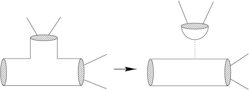
Figure 1: A type-I diagram with Euler characteristic $\chi=-1$. This contributes to the $(tr{\cal F}^{2})^{2}$ piece of the effective action, only in degeneration limits such as the one depicted above.

Let us now proceed to evaluate this expression. The fundamental domain integrals can be performed explicitly by using the formula [94]

$$\int_{F}{d^{2}\tau\over\tau_{2}^{2}}({\hat{E}}_{2})^{r}\Phi_{r}=\ {\pi\over 3(r+1)}[c_{0}-24(r+1)c_{-1}]$$ (5.4.6)

where

$$\Phi_{r}(q)=\sum_{n=-1}^{\infty}c_{n}q^{n}$$ (5.4.7)

is any modular form of weight $-2r$ which is holomorphic everywhere except possibly for a simple pole at zero. As for the strip integration, it picks up only the ${\cal O}(q^{0})$ term in the expansion of ${\cal A}$. Modulo the non-holomorphic regularization, only the SO(32) gauge bosons contribute to the elliptic genus at this order, in agreement precisely with the result of the type-I side! For $k\geq 1$ let us define more generally

$$\;\int_{0}^{\infty}{d\tau_{2}\over\tau_{2}^{1+k}}\sum_{j\not=0}e^{-2\pi L^{2}j^{2}/\tau_{2}}={2\Gamma(k)\zeta(2k)\over(2\pi L^{2})^{k}}\ \equiv{N_{k}\over L^{2k}},$$ (5.4.8)

where $L$ is the radius of the compactification circle. The one-loop SO(32) heterotic action takes finally the form

 

$${{\cal I}^{het}=-{V^{(10)}\over 2^{10}\pi^{6}}}$$

  (5.4.9)

To simplify notation we have written here ${\cal F}^{4}$ instead of $t_{8}\;tr{\cal F}^{4}$, $({\cal F}^{2})^{2}$ instead of $t_{8}\;tr{\cal F}^{2}tr{\cal F}^{2}$ etc.

We have expressed the result as an expansion in inverse powers of the compactification volume. Since the heterotic/type-I duality map transforms ($\sigma$-model) length scales as

$$L^{2}_{h}=L^{2}_{I}/\lambda_{I}$$ (5.4.10)

with $\lambda_{I}$ the open-string loop counting parameter, this expansion can be translated to a genus expansion on the type-I side. The Euler number of an non-orientable surface is given by $\chi=2-2g-B-C$ where $g$ is the number of holes, $B$ the number of boundaries and $C$ the number of cross-caps. The leading term corresponds to the disk and projective plane diagrams and is completely fixed by ten-dimensional supersymmetry and anomaly cancellation [69]. To check this, one must remember to transform the metric in both $V^{(10)}$ and the tensor $t_{8}$ appropriately. Notice that the type-I sphere diagram, which is the same as in type IIB, only contributes to the $J_{0}$ invariant which we are not considering here. The subleading o($L^{-2}$) terms correspond to the annulus, Möbius strip, Klein bottle and torus diagrams, all with $\chi=0$. For zero background curvature these agree with the type-I calculation [31] as described in section 5.3.

The last two terms in the expansion (5.4.9) correspond to diagrams with $\chi=-1,-2$. These contributions must be there if the duality map of ref. [90] does not receive higher-order corrections. Such corrections could anyway always be absorbed by redefining fields on the type-I side, so that if duality holds, there must exist some regularization scheme in which these higher-genus contributions do arise. These terms do on the other hand come from the boundary of moduli space. For instance the $\chi=-1$ contribution to the $({\cal F}^{2})^{2}$ term comes from the boundary of moduli space shown in figure 1. It could thus be conceivably eliminated in favour of some lower-dimension operators in the effective action.

It is in any case striking that a single heterotic diagram contains contributions from different topologies on the type-I side. Notice in particular that the divergent $w=0$ term in the one-loop field theoretic calculation, regularized on the heterotic side by replacing the strip by a fundamental domain, is regularized on the type-I side by replacing the annulus by the disk.

5.5 Two-torus Compactification

The next simplest situation corresponds to compactification on a two-dimensional torus. There are in this case world-sheet instanton contributions on the heterotic side, and our aim in this and the following sections will be to understand them as (Euclidean) D-string trajectory contributions on the type-I side. The discussion can be extended with little effort to toroidal compactifications in lower than eight dimensions. New effects are only expected to arise in four or fewer uncompactified dimensions, where the solitonic heterotic instantons or, equivalently, the type-I D5-branes can contribute.

The target-space torus is characterized by two complex moduli, the Kähler-class

$$T=T_{1}+iT_{2}=\frac{1}{\alpha^{\prime}}(B_{89}+i\sqrt{G})$$ (5.5.11)

and the complex structure

$$U=U_{1}+iU_{2}=(G_{89}+i\sqrt{G})/G_{88}\ ,$$ (5.5.12)

where $G_{\mu\nu}$ and $B_{\mu\nu}$ are the $\sigma$-model metric and antisymmetric tensor on the heterotic side. The one-loop thresholds now read

$${\cal I}^{het}={V^{(8)}\over 2^{9}\pi^{4}}\;\int_{F}{d^{2}\tau\over\tau_{2}}\Gamma_{2,2}\;{\cal A}({\cal F},{\cal R},\tau)\ ,$$ (5.5.13)

where the lattice sum takes the form [101]

$${\Gamma_{2,2}}={T_{2}\over\tau_{2}}\times\sum_{M\in{\rm Mat}(2\times 2,{{Z}})}e^{2\pi iT{\rm det}M}e^{-\frac{\pi T_{2}}{\tau_{2}U_{2}}\big{|}(1\;U)M\big{(}{\tau\atop-1}\big{)}\big{|}^{2}}\,.$$ (5.5.14)

The exponent in the above sum is (minus) the Polyakov action,

$$S_{\rm Polyakov}={1\over 4\pi\alpha^{\prime}}\int d^{2}\sigma(\sqrt{g}G_{\mu\nu}g^{\alpha\beta}\partial_{\alpha}X^{\mu}\partial_{\beta}X^{\nu}+iB_{\mu\nu}\epsilon^{\alpha\beta}\partial_{\alpha}X^{\mu}\partial_{\beta}X^{\nu})\ ,$$ (5.5.15)

evaluated for the topologically non-trivial mapping of the string world-sheet onto the target-space torus,

$$\left(\matrix{X^{8}\cr X^{9}\cr}\right)=M\left(\matrix{\sigma^{1}\cr\sigma^{2}\cr}\right)\equiv\left(\matrix{m_{1}&n_{1}\cr m_{2}&n_{2}\cr}\right)\left(\matrix{\sigma^{1}\cr\sigma^{2}\cr}\right)\ \,.$$ (5.5.16)

The entries of the matrix $M$ are integers, and both target-space and world-sheet coordinates take values in the (periodic) interval $(0,2\pi]$. To verify the above assertion one needs to use the metrics

$$G_{\mu\nu}={\alpha^{\prime}T_{2}\over U_{2}}\;\left(\matrix{1&U_{1}\cr U_{1}&|U|^{2}\cr}\right)\;,\ \ \ g^{\alpha\beta}={1\over\tau_{2}^{\ 2}}\;\left(\matrix{|\tau|^{2}&-\tau_{1}\cr-\tau_{1}&1\cr}\right)\ .$$ (5.5.17)

The Polyakov action is invariant under global reparametrizations of the world-sheet,

$$\left(\matrix{\sigma^{1}\cr\sigma^{2}\cr}\right)\rightarrow\left(\matrix{a&-b\cr-c&d\cr}\right)\left(\matrix{\sigma^{1}\cr\sigma^{2}\cr}\right)\ ,$$ (5.5.18)

which transform

$$\tau\rightarrow{a\tau+b\over c\tau+d}\ ,\ \ {\rm and}\ \ M\rightarrow M\ \left(\matrix{d&b\cr c&a\cr}\right)\ \,.$$ (5.5.19)

Following Dixon, Kaplunovsky and Louis [101], we decompose the set of all matrices $M$ into orbits of PSL(2,Z), which is the group of the above transformations up to an overall sign. There are three types of orbits,

 

$${{}{\rm invariant}:\ M=0}$$

 

A canonical choice of representatives for the degenerate orbits is

$$M=\left(\matrix{0&j_{1}\cr 0&j_{2}\cr}\right)$$ (5.5.20)

where the integers $j_{1},j_{2}$ should not both vanish, but are otherwise arbitrary. Distinct elements of a degenerate orbit are in one-to-one correspondence with the set ${\cal S}$, i.e. with modular transformations that map the fundamental domain inside the strip, as in section 5.4. In what concerns the non-degenerate orbits, a canonical choice of representatives is

$$M=\pm\left(\matrix{k&j\cr 0&p\cr}\right)\ \ {\rm with}\ \ 0\leq j<k\quad,\quad\ p\not=0\ .$$ (5.5.21)

Distinct elements of a non-degenerate orbit are in one-to-one correspondence with the fundamental domains of $\tau$ in the upper-half complex plane.

Trading the sum over orbit elements for an extension of the integration region of $\tau$, we can thus express eqs. (5.5.13,5.5.14) as follows

 

$${{\cal I}^{het}=-{V^{(8)}T_{2}\over 2^{9}\pi^{4}}\times}$$

  (5.5.22)

The three terms inside the curly brackets are constant, power-suppressed and exponentially-suppressed in the large compactification-volume limit. They correspond to tree-level, higher perturbative and non-perturbative, respectively, contributions on the type-I side. The discussion of the perturbative contributions follows exactly the analogous discussion in section 5.4. The only difference is the replacement of eq. (5.4.8) by

 

$${\int_{0}^{\infty}{d\tau_{2}\over\tau_{2}^{\ 1+k}}\;\sum_{(j_{1},j_{2})\neq(0,0)}e^{-\frac{\pi T_{2}}{\tau_{2}U_{2}}\big{|}j_{1}+j_{2}U\big{|}^{2}}=}$$

  (5.5.23)

where $E(U,k)$ are generalized Eisenstein series. In the open-string channel of the type-I side this takes into account properly the (double) sum over Kaluza-Klein momenta [31]. Notice that the holomorphic anomalies in ${\cal A}$ lead again to higher powers of the inverse volume, which translate to higher-genus contributions on the type-I side. Notice also that the $k=1$ term has a logarithmic infrared divergence, which must be regularized appropriately, as discussed in the introduction.

We turn now to the novel feature of eight dimensions, namely the contributions of world-sheet instantons. Plugging in the expansion (5.2.8) of the elliptic genus, we are lead to consider the integrals

$$I_{n,r}=\int_{{C}^{+}}{d^{2}\tau\over\tau_{2}^{\ 2}}\;e^{-\frac{\pi T_{2}}{\tau_{2}U_{2}}\big{|}k\tau-j-pU\big{|}^{2}}\;{1\over\tau_{2}^{\ r}}e^{2i\pi\tau n}$$ (5.5.24)

Doing first the (Gaussian) $\tau_{1}$ integral, one finds after some rearrangements

$$I_{n,r}={1\over k}\sqrt{U_{2}\over T_{2}}e^{2i\pi n({j+pU_{1}\over k})}e^{2\pi kpT_{2}}\int_{0}^{\infty}{d\tau_{2}\over\tau_{2}^{3/2+r}}e^{-{\pi T_{2}\over U_{2}}(k+{nU_{2}\over kT_{2}})^{2}\tau_{2}}e^{-\pi p^{2}T_{2}U_{2}/\tau_{2}}$$ (5.5.25)

The $\tau_{2}$ integration can now be done using the formula

$$\int_{0}^{\infty}{dx\over x^{3/2+r}}e^{-ax-b/x}=\left(-{\partial\over\partial b}\right)^{r}\sqrt{\pi\over b}\;e^{-2\sqrt{ab}}$$ (5.5.26)

where $a={\pi T_{2}\over U_{2}}(k+{nU_{2}\over kT_{2}})^{2}$ and $b=\pi p^{2}T_{2}U_{2}$ are both proportional to the volume of the compactification torus. The leading term in the large-volume limit is obtained when all derivatives hit the exponential in the above expression. Using (5.5.26) we find

$$I_{n,r}={1\over k|p|T_{2}}\left({k\over|p|U_{2}}\right)^{r}\;e^{2\pi k(p-|p|)T_{2}}e^{2i\pi n[{j+pU_{1}\over k}+i|p|{U_{2}\over k}]}\;\Bigl{(}1+{\rm o}({1\over T_{2}})\Bigr{)}$$ (5.5.27)

and plugging back into eq. (5.5.22) we obtain

$${\cal I}^{het}_{inst}\simeq-{2V^{(10)}\over 2^{10}\pi^{6}}\sum_{{0\leq j<k}\atop{p>0}}{1\over kpT_{2}}\;e^{2\pi iTpk}\;{\cal A}\left({j+pU\over k}\right)+\ {\rm c.c.}$$ (5.5.28)

This equality is exact for the holomorphic parts of the elliptic genus. Correction terms have the form of an order-$r_{max}$ polynomial in inverse powers of the volume, as we will discuss in a minute.

Expression (5.5.28) has an elegant rewriting in terms of Hecke operators $H_{N}$ [102, 103]. On any modular form $\Phi_{r}(z)$ of weight $-2r$, the action of a Hecke operator, defined by [102]

$$H_{N}[\Phi_{r}](z)={1\over N^{2r+1}}\sum_{k,p>0\atop kp=N}\sum_{0\leq j<k}k^{2r}\;\Phi_{r}\left(pz+j\over k\right)\ ,$$ (5.5.29)

gives another modular form of the same weight. The Hecke operator is self-adjoint with respect to the inner product defined by integration of modular forms on a fundamental domain. Using the above definition one finds

$${\cal I}^{het}_{inst}\simeq-{2V^{(10)}\over 2^{10}\pi^{6}}\sum_{N=1}^{\infty}{1\over T_{2}}\;e^{2\pi iNT}\;H_{N}[{\cal A}](U)+{\rm c.c.}$$ (5.5.30)

In the above form the result might be easier to compare with a calculation based on the heterotic matrix string theory [104].

Figure 2: Embedding of the lattice $\Gamma^{\prime}$ (D1-brane) in the lattice $\Gamma$ (target space torus).

Let us complete now the calculation, by taking into account the sub-leading terms in the large-volume limit. Using eq. (5.5.26) we can in fact evaluate explicitly the integrals (5.5.24). After some long but straightforward algebra the correction terms can all be expressed in terms of the induced moduli

$${\cal U}={j+pU\over k}\ \ \ {\rm and}\ \ \ {\cal T}=kpT\ .$$ (5.5.31)

$$I_{n,1}\to I_{n,1}\times\left(\;1+{1\over{\cal T}_{2}}(n{\cal U}_{2}+{1\over 2\pi})\right)\ ,$$ (5.5.32)

$$I_{n,2}\to I_{n,2}\times\left(\;1+{1\over{\cal T}_{2}}(2n{\cal U}_{2}+{3\over 2\pi})+{1\over{\cal T}_{2}^{2}}(n^{2}{\cal U}_{2}^{2}+{3n{\cal U}_{2}\over 2\pi}+{3\over 4\pi^{2}})\right)\ .$$ (5.5.33)

These terms can be rewritten elegantly by using the operator

$$\mathchoice{\vbox{\vbox{\hrule height=0.4pt\hbox{\vrule width=0.4pt,height=6.0pt\kern 6.0pt\vrule width=0.4pt} \hrule height=0.4pt}}}{\vbox{\vbox{\hrule height=0.4pt\hbox{\vrule width=0.4pt,height=6.0pt\kern 6.0pt\vrule width=0.4pt} \hrule height=0.4pt}}}{\vbox{\vbox{\hrule height=0.3pt\hbox{\vrule width=0.3pt,height=2.1pt\kern 2.1pt\vrule width=0.3pt} \hrule height=0.3pt}}}{\vbox{\vbox{\hrule height=0.3pt\hbox{\vrule width=0.3pt,height=1.5pt\kern 1.5pt\vrule width=0.3pt} \hrule height=0.3pt}}}\equiv{\cal U}_{2}^{2}\partial_{\cal U}{\bar{\partial}}_{\cal U}$$ (5.5.34)

This is a modular invariant operator, which annihilates holomorphic forms. The correction terms for all $r=0,1,2$ are summarized by the expression

$${\cal U}_{2}^{\ r}e^{-2i\pi{\cal U}n}\left(1+{1\over\pi{\cal T}_{2}}\mathchoice{\vbox{\vbox{\hrule height=0.4pt\hbox{\vrule width=0.4pt,height=6.0pt\kern 6.0pt\vrule width=0.4pt} \hrule height=0.4pt}}}{\vbox{\vbox{\hrule height=0.4pt\hbox{\vrule width=0.4pt,height=6.0pt\kern 6.0pt\vrule width=0.4pt} \hrule height=0.4pt}}}{\vbox{\vbox{\hrule height=0.3pt\hbox{\vrule width=0.3pt,height=2.1pt\kern 2.1pt\vrule width=0.3pt} \hrule height=0.3pt}}}{\vbox{\vbox{\hrule height=0.3pt\hbox{\vrule width=0.3pt,height=1.5pt\kern 1.5pt\vrule width=0.3pt} \hrule height=0.3pt}}}+{1\over 2}{1\over\pi^{2}{\cal T}_{2}^{2}}(\mathchoice{\vbox{\vbox{\hrule height=0.4pt\hbox{\vrule width=0.4pt,height=6.0pt\kern 6.0pt\vrule width=0.4pt} \hrule height=0.4pt}}}{\vbox{\vbox{\hrule height=0.4pt\hbox{\vrule width=0.4pt,height=6.0pt\kern 6.0pt\vrule width=0.4pt} \hrule height=0.4pt}}}{\vbox{\vbox{\hrule height=0.3pt\hbox{\vrule width=0.3pt,height=2.1pt\kern 2.1pt\vrule width=0.3pt} \hrule height=0.3pt}}}{\vbox{\vbox{\hrule height=0.3pt\hbox{\vrule width=0.3pt,height=1.5pt\kern 1.5pt\vrule width=0.3pt} \hrule height=0.3pt}}}^{2}-\mathchoice{\vbox{\vbox{\hrule height=0.4pt\hbox{\vrule width=0.4pt,height=6.0pt\kern 6.0pt\vrule width=0.4pt} \hrule height=0.4pt}}}{\vbox{\vbox{\hrule height=0.4pt\hbox{\vrule width=0.4pt,height=6.0pt\kern 6.0pt\vrule width=0.4pt} \hrule height=0.4pt}}}{\vbox{\vbox{\hrule height=0.3pt\hbox{\vrule width=0.3pt,height=2.1pt\kern 2.1pt\vrule width=0.3pt} \hrule height=0.3pt}}}{\vbox{\vbox{\hrule height=0.3pt\hbox{\vrule width=0.3pt,height=1.5pt\kern 1.5pt\vrule width=0.3pt} \hrule height=0.3pt}}}/2)\right)\ {\cal U}_{2}^{\;-r}e^{2i\pi{\cal U}n}.$$ (5.5.35)

The instanton sum is modified accordingly to

$${\cal I}^{het}_{inst}=-{2V^{(10)}\over 2^{10}\pi^{6}}\sum_{instantons}{1\over{\cal T}_{2}}\;e^{2\pi i{\cal T}}\;\left(1+{1\over\pi{\cal T}_{2}}\mathchoice{\vbox{\vbox{\hrule height=0.4pt\hbox{\vrule width=0.4pt,height=6.0pt\kern 6.0pt\vrule width=0.4pt} \hrule height=0.4pt}}}{\vbox{\vbox{\hrule height=0.4pt\hbox{\vrule width=0.4pt,height=6.0pt\kern 6.0pt\vrule width=0.4pt} \hrule height=0.4pt}}}{\vbox{\vbox{\hrule height=0.3pt\hbox{\vrule width=0.3pt,height=2.1pt\kern 2.1pt\vrule width=0.3pt} \hrule height=0.3pt}}}{\vbox{\vbox{\hrule height=0.3pt\hbox{\vrule width=0.3pt,height=1.5pt\kern 1.5pt\vrule width=0.3pt} \hrule height=0.3pt}}}+{1\over 2}{1\over\pi^{2}{\cal T}_{2}^{2}}(\mathchoice{\vbox{\vbox{\hrule height=0.4pt\hbox{\vrule width=0.4pt,height=6.0pt\kern 6.0pt\vrule width=0.4pt} \hrule height=0.4pt}}}{\vbox{\vbox{\hrule height=0.4pt\hbox{\vrule width=0.4pt,height=6.0pt\kern 6.0pt\vrule width=0.4pt} \hrule height=0.4pt}}}{\vbox{\vbox{\hrule height=0.3pt\hbox{\vrule width=0.3pt,height=2.1pt\kern 2.1pt\vrule width=0.3pt} \hrule height=0.3pt}}}{\vbox{\vbox{\hrule height=0.3pt\hbox{\vrule width=0.3pt,height=1.5pt\kern 1.5pt\vrule width=0.3pt} \hrule height=0.3pt}}}^{2}-\mathchoice{\vbox{\vbox{\hrule height=0.4pt\hbox{\vrule width=0.4pt,height=6.0pt\kern 6.0pt\vrule width=0.4pt} \hrule height=0.4pt}}}{\vbox{\vbox{\hrule height=0.4pt\hbox{\vrule width=0.4pt,height=6.0pt\kern 6.0pt\vrule width=0.4pt} \hrule height=0.4pt}}}{\vbox{\vbox{\hrule height=0.3pt\hbox{\vrule width=0.3pt,height=2.1pt\kern 2.1pt\vrule width=0.3pt} \hrule height=0.3pt}}}{\vbox{\vbox{\hrule height=0.3pt\hbox{\vrule width=0.3pt,height=1.5pt\kern 1.5pt\vrule width=0.3pt} \hrule height=0.3pt}}}/2)\right)\ {\cal A}({\cal U})\ +\ {\rm c.c.}\ .$$ (5.5.36)

One final rearrangement puts this to the form

$${\cal I}^{het}_{inst}=-{2V^{(10)}\over 2^{10}\pi^{6}}\sum_{instantons}{1\over{\cal T}_{2}}\;e^{2\pi i{\cal T}}\;\left(\sum_{s=0}^{\infty}{1\over s!}{1\over{\cal T}_{2}^{s}}(-iD)^{s}({\cal U}_{2}^{2}{\bar{\partial}}_{\cal U})^{s}\right)\ {\cal A}({\cal U})\ +\ {\rm c.c.}\ .$$ (5.5.37)

where here $D$ is the covariant derivative, which acting on a modular form $\Phi_{r}$ of weight $-2r$ gives a form of weight $-2r+2$,

$$D\Phi_{r}=\left({i\over\pi}\partial_{\cal U}-{r\over\pi{\cal U}_{2}}\right)\Phi_{r}\ .$$ (5.5.38)

The virtue of this last rewriting is that the $s$th operator in the sum annihilates explicitly the first $s$ terms in the expansion of the elliptic genus in powers of ${1\over{\cal U}_{2}}$. From the general form of ${\cal A}$, eq. (5.2.8) we conclude that only the terms with $s\leq 2$ ($s\leq 1$) contribute in the case of sixteen (eight) unbroken real supercharges. The modular-invariant descendants of the genus, obtained by applying the $s$th operator on ${\cal A}$, determine in fact the corrections to other dimension-eight operators in the effective action. The full effective action can be expressed in terms of generalized holomorphic prepotentials, a result that we will not develop further here.

5.6 D-instanton Interpretation

We would now like to understand the above result from the perspective of type-I string theory. The world-sheet instantons on the heterotic side map to D-brane instantons, that is Euclidean trajectories of D-strings wrapping non-trivially around the compactification torus. A Euclidean trajectory described by eq. (5.5.16) defines a sublattice ($\Gamma^{\prime}$) of the compactification lattice ($\Gamma$). If ${\bf e}_{i=1,2}$ are the two vectors spanning $\Gamma$, then $\Gamma^{\prime}$ is spanned by the vectors ${\bf e^{\prime}}_{i}=M_{ji}{\bf e_{j}}$ (figure 2). Under a change of basis for $\Gamma$ ($\Gamma^{\prime}$) the matrix $M$ transforms by left (right) multiplication with the appropriate elements of SL(2,Z). Using reparametrizations of the world-sheet we can thus bring the basis ${\bf e^{\prime}_{i}}$ into the canonical form, eq. (5.5.21), as described in the previous section (see also figure 2).

Now the key remark is that on the heterotic world-sheet we have an induced complex structure and Kähler modulus, which for positive $p$ are given by

$${\cal U}={j+pU\over k}\ \ \ {\rm and}\ \ \ {\cal T}=kpT\ .$$ (5.6.1)

For negative $p$’s, describing anti-instantons, we must take the absolute value of $p$ and complex conjugate these expressions. One can check these facts by inspection of figure 2, or by computing explicitly the pull-backs of the metric and antisymmetric tensor field,

$$\hat{G}_{\alpha\beta}=G_{\mu\nu}\partial_{\alpha}X^{\mu}\partial_{\beta}X^{\nu}\,\,\,,\,\,\,\hat{B}_{\alpha\beta}=B_{\mu\nu}\partial_{\alpha}X^{\mu}\partial_{\beta}X^{\nu}\ .$$ (5.6.2)

Notice that $N=kp$ is the total number of times the world-sheet wraps around the compactification torus. In terms of induced moduli the instanton sum (5.5.28) takes the form

$${\cal I}_{inst}\simeq-{2V^{(10)}\over 2^{10}\pi^{6}}\sum_{instantons}{1\over{\cal T}_{2}}\;e^{2\pi i{\cal T}}\;{\cal A}({\cal U})+{\rm c.c.}\ .$$ (5.6.3)

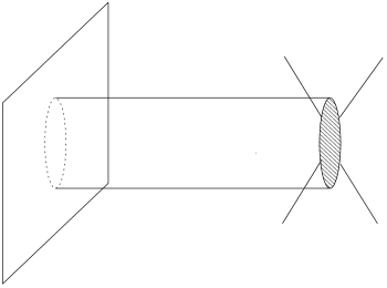
Figure 3: A D1-brane instanton correction to $trF^{4}$.

The various terms of this expression have a simple interpretation on the type-I side. The action of a wrapped D-string is [105]

$$S_{\rm D-string}={1\over 2\pi\alpha^{\prime}\lambda_{I}}\int d^{2}\sigma\sqrt{|{\rm det}\hat{G}_{I}|}-{i\over 2\pi\alpha^{\prime}}\int\hat{B}_{I}$$ (5.6.4)

where $B_{I}$ is the type-I 2-form coming from the RR sector. Using the heterotic/type-I map

$${\cal T}_{2}^{het}={\cal T}_{2}^{I}/\lambda_{I}\ ,\ \ B^{het}=B^{I}$$ (5.6.5)

and the fact that the world-sheet area of the D-string is $4\pi^{2}{\cal T}_{2}^{I}$, we see that the exponential of this Nambu-Goto action reproduces exactly the exponential in the instanton sum, eq. (5.6.3). The inverse factor of the volume comes from the integration of the longitudinal translation zero modes. Finally the elliptic genus of the D-brane complex structure, should come from the functional integration over the (second quantized) string fields in the instanton background. A typical diagram contributing to the ${\cal F}^{4}$ coupling is shown in figure 3. For the purely holomorphic pieces of the elliptic genus the result is topological, so it should be expected to coincide with the heterotic $\sigma$-model calculation of refs. [93, 94, 33, 34]. Put differently, massive string modes and higher-order terms in the effective D-string action are expected to play no role in the calculation.

From the type-I point of view expression (5.5.28) is, however, still somewhat unnatural. The three configurations of figure 4 correspond to the same (singular) effective-field-theory solution, characterized by two units of the appropriate Ramond-Ramond charge. Why then should we count them as distinct saddle points? Furthermore, the fluctuations of the double D-brane are not described by the usual heterotic $\sigma$-model, but by its (non-abelian) $2\times 2$-matrix generalization [106, 104], which is the low-energy limit of an open string theory. Why should then the result be proportional to the conventional elliptic genus?

In order to answer these questions it is convenient to put the effective action (5.5.28) in the more elegant form

$${\cal I}^{\rm inst}=-{V^{(8)}\over 2^{8}\pi^{4}}\sum_{N=1}^{\infty}\;e^{2\pi iNT}{\cal H}_{N}{\hat{\cal A}}(U)\ +{\rm c.c.},$$ (5.6.6)

with

$${\cal H}_{N}{\hat{\cal A}}(U)\equiv{1\over N}\sum_{kp=N\atop 0\leq j<k}{\hat{\cal A}}\left({j+pU\over k}\right)\ .$$ (5.6.7)

We have just seen the geometric interpretation of the Hecke operators in terms of inequivalent N-fold wrappings of the torus by the (heterotic) world-sheet. We will now describe an alternative interpretation, more appropriate on the type-I side, in terms of the moduli space of instantons [107, 18]. The key will be to treat this moduli space as a symmetric orbifold [108, 109, 103], an idea that is more familiar in the context of black-hole state counting [110].

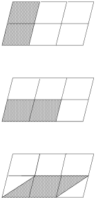
Figure 4: The three distinct ways in which the (shaded) heterotic world-sheet can wrap twice around the target-space torus.

The low-energy fluctuations around a configuration of $N$ instantonic D-branes are described by a heterotic matrix $\sigma$-model, with local SO(N) symmetry on the world-sheet [106, 104]. The coupling of a constant target-space background field reads

$$\delta I_{\sigma}\ \propto\ \int\;F_{ij}^{\alpha}T_{\alpha}^{rs}\ \lambda_{r}^{\;T}\ \Bigl{[}X^{i}{\bar{D}}X^{j}-{1\over 8}S^{\dagger}\gamma^{ij}S\Bigr{]}\lambda_{s}\ .$$

Under the SO(N) gauge symmetry the supercoordinates $X^{i}$ and $S^{\dot{a}}$ are symmetric matrices, the current-algebra fermions $\lambda_{r}$ are vectors, and ${\bar{D}}$ is the antiholomorphic covariant derivative. We are interested in the functional integral of this $\sigma$-model, with four insertions of $\delta I_{\sigma}$. Notice that contributions of massive string modes are expected to cancel out for this special amplitude, justifying the reduction of the calculation to the matrix model.

The moduli space of this multi-instanton has a Coulomb branch along which the $X^{i}$ have diagonal expectation values. In the type $I^{\prime}$ language these label the positions of N D0-particles on the orientifold plane . At a generic point in this moduli space there are 8N fermionic zero modes, corresponding to the diagonal components of the matrices $S^{\dot{a}}$. Since only eight of them can be absorbed by the insertions of the vertex $\delta I_{\sigma}$, one would naively conclude that the sectors $N>1$ do not contribute. This is wrong because of the residual gauge symmetry that permutes the positions of the D-branes. The moduli space is thus a symmetric orbifold and there are potential contributions from its fixed points.

Let us illustrate how this works in the case of two instantons. The massless fluctuations of the double D-brane are described by a conformal field theory with target space ${\cal M}\times{\cal M}/Z_{2}$, where ${\cal M}$ is the (transverse) target space of the heterotic string, and $Z_{2}$ is the exchange symmetry. There are four contributions to the amplitude, corresponding to the four boundary conditions on the torus. The untwisted sector has $2\times 8$ fermionic zero modes and does not contribute. The contribution of the remaining three sectors is proportional to

$${\hat{\cal A}}(2U)+{\hat{\cal A}}\Bigl{(}{U\over 2}\Bigr{)}+{\hat{\cal A}}\Bigl{(}{U+1\over 2}\Bigr{)}\ ,$$

as can be shown using standard $Z_{2}$-orbifold techniques. This is precisely the action of the Hecke operator ${\cal H}_{2}$, corresponding to the sum over the three surfaces of figure 1. The overall coefficient also checks, including the orbifold normalization of ${1\over 2}$, and the simple factor of the transverse volume characteristic of the twisted-sector contributions.

The generalization to any $N$ is straightforward. The target space is now the symmetric orbifold

$$\underbrace{{\cal M}\times...\times{\cal M}}_{\rm N\ times}\bigg{/}S_{N}$$

The non-vanishing contributions to the amplitude come from those boundary conditions for which only the trace part of $S^{\dot{a}}$ is (doubly) periodic on the torus. Up to a common overall normalization, the result is given by ${\cal H}_{N}{\hat{\cal A}}(U)$, which is the matrix-model generalization of ${\hat{\cal A}}$. The non-perturbative type-I effective action is obtained by summing over all N, as in expression (5.6.6).

5.7 Heterotic/Type-I duality in $D<8$

We will now discuss heterotic thresholds in toroidal compactifications to $D<8$. As we argued earlier, if $D>4$ then the heterotic result is still one-loop only and can be evaluated. Using heterotic/type-I duality we find again the non-perturbative type-I corrections and we show that their corresponding D1-brane interpretation is in agreement with the D1-brane rules given in Section 5.6.

Our starting point is the general form of the one-loop thresholds

$${\cal I}^{\rm het}_{D}=-{\cal N}_{D}\int_{{\cal F}}{d^{2}\tau\over\tau_{2}^{2}}\;(\tau_{2}^{d/2}\Gamma_{d,d}(G,B))\ {\cal A}(\tau)\,,$$ (5.7.1)

where the $D+d=10$ and the $d$-dimensional lattice sum $\Gamma_{d,d}$ is given by

$$\Gamma_{d,d}(G,B)={\sqrt{G}\over\tau_{2}^{d/2}}\sum_{m^{i},n^{i}\in{Z}}\exp\left[-{\pi\over\tau_{2}}(G+B)_{ij}(m^{i}+n^{i}\tau)(m^{j}+n^{j}\bar{\tau})\right]\,,$$ (5.7.2)

where $G$ and $B$ are the $d$-dimensional metric and antisymmetric tensor respectively.

The corresponding integral (5.7.1) can be evaluated again, using the method of orbits. We refer to [19] for the main steps, and quote here only the result of the non-degenerate orbit, which comprises the type-I instantonic contributions:

$${\cal I}_{\rm inst}=-2{\cal N}_{D}\sum_{s=0}^{\nu_{\rm max}}\left({3\over 2\pi}\right)^{s}\sum_{m,n}^{\prime}{\sqrt{G}\over(T^{m,n}_{2})^{s+1}}e^{2\pi iT^{m,n}}{\cal A}_{s}(U^{m,n})$$ (5.7.3)

Here, the induced Kähler and complex structure moduli are given by

$$T^{m,n}=mBn+i\sqrt{(mGm)(nGn)-(mGn)^{2}}\;\;\;\;\;\;\;\;\;\;\;\;\;\;\;\;\;$$ (5.7.4a)

$$U^{m,n}=\left(-mGn+i\sqrt{(mGm)(nGn)-(mGn)^{2}}\;\right)/nGn$$ (5.7.4b)

and the $\sum_{m,n}^{\prime}$ is over the non-degenerate orbits, which are parametrized by the following integer-valued $2\times d$ matrices

$$\mbox{non-degenerate orbit}:\;\;\;\;A^{T}=\left(\matrix{n_{1}&\ldots&n_{k}&0&\ldots&0\cr m_{1}&\ldots&m_{k}&m_{k+1}&\ldots&m_{d}\cr}\right)\;\;\;\;\;\;\;\;\;\;\;\;\;\;\;\;\;\;\;\;\;\;\;\;\;\;\;\;\;\;\;\;$$ (5.7.5a)

$$\;\;\;\;\;\;\;\;\;\;\;\;\;\;\;\;\;\;\;\;\;\;\;\;\;\;\;\;\;\;\;\;\;\;1\leq k<d~{}~{},~{}~{}n_{k}>m_{k}\geq 0~{}~{},~{}~{}(m_{k+1},\ldots,m_{d})\neq(0,\ldots,0)\,.$$ (5.7.5b)

Note that for $d=2$ the general result (5.7.3) reduces to the one given in (5.5.28).

Turning to the D1-brane interpretation of the result, we first wish to establish that the exponential factor $e^{2\pi iT^{m,n}}$ agrees with the classical action of a D1-brane. The map that describes the wrapping of the D1-brane world-sheet around a 2-cycle in the $d$-torus is

$$X^{i}=n_{i}\sigma_{1}+m_{i}\sigma_{2}~{}~{},~{}~{}i=1\ldots d\,,$$ (5.7.6)

where $X^{i}$ are the coordinates on $T^{d}$ and $\sigma_{1,2}$ the D1-brane coordinates. We observe that modular transformations on the D1-brane coordinates act on the matrix $A$ that enters (5.7.6)

$$A=\left(\matrix{n_{1}&m_{1}\cr\vdots&\vdots\cr n_{d}&m_{d}\cr}\right)$$ (5.7.7)

by right SL(2,ℤ) transformations, which forces us to pick the representative configurations described by the matrices in (5.7.5b).

In terms of the matrix $M_{I}^{i}=(A_{i}^{I})^{T}=(n^{i},m^{i})$, $I=1,2$, we see that the induced metric and antisymmetric tensor fields are

$$\hat{G}_{IJ}=M_{I}^{i}G_{ij}M_{J}^{j}~{}~{},~{}~{}\hat{B}_{IJ}=M_{I}^{i}B_{ij}M_{J}^{j}\,.$$ (5.7.8)

In particular, going through the same steps as in Section 5.6, we find from the D1-brane classical action (5.6.4) and (5.7.4b), (5.7.8) that $e^{-S_{\rm class}}$ precisely reduces to the exponential factor $e^{2\pi iT^{m,n}}$, which is to be summed over the ranges indicated in (5.7.5b). We also note that we correctly observe the overall factor $\sqrt{G}/\sqrt{\hat{G}}=\sqrt{G}/T^{m,n}_{2}$. Moreover, the fluctuation determinant is evaluated at the induced modulus $U^{m,n}$ of the wrapped D1-brane.

This establishes the claim that the D1-brane rules in $D<8$ are consistent with those obtained for $D=8$. In summary, we have found the intuitively expected result: The situation is as in eight dimensions with the difference that now the D1 world-volume can wrap in many more ways on submanifolds of $T^{10-D}$.

In the eight-dimensional case it was shown [18, 19] that differential equations satisfied by the (2,2) toroidal lattice sum translate into recursion relations for the thresholds, which can be solved in terms of holomorphic prepotentials. There is a generalization of such equations for the $(d,d)$ toroidal lattice sum.

It was noted in Refs. [56, 111] that the toroidal partition function $\Gamma_{d,d}(G,B;\tau)$ satisfies the following differential equation:

$$\left[\left(\sum_{i\leq j}G_{ij}{\partial\over\partial G_{ij}}+{1-d\over 2}\right)^{2}+\frac{1}{2}\sum_{ijkl}G_{ik}G_{jl}{\partial^{2}\over\partial B_{ij}\partial B_{kl}}-\frac{1}{4}-4\tau_{2}^{2}{\partial^{2}\over\partial\tau\partial\bar{\tau}}\right]\Gamma_{d,d}(G,B;\tau)=0$$ (5.7.9)

which in the case $d=2$ reduces to

$$\left[T_{2}^{2}\partial_{T}\partial_{\bar{T}}-\tau_{2}^{2}\partial_{\tau}\partial_{\bar{\tau}}\right]\Gamma_{2,2}(T,U;\tau)=0\,.$$ (5.7.10)

However, the general differential equation in (5.7.9) is not invariant under the full $O(d,d,Z)$ duality group. It may be verified that it is invariant under integer $B$ shifts and $SL(d,Z)$ basis changes, but there is no invariance under the remaining generators of the duality group, which are the inversion and factorized duality. The latter two transformations act on the matrix $E\equiv G+B$ as follows:

$$E\rightarrow E^{-1}~{}~{},~{}~{}E\rightarrow[(1-e_{i})E+e_{i}][e_{i}E+(1-e_{i})]^{-1}~{}~{},~{}~{}(e_{i})_{k,l}=\delta_{ik}\delta_{il}\,.$$ (5.7.11)

For example, in the $d=2$ case the factorized dualities correspond to $T\rightarrow U$ and $T\rightarrow 1/U$ for $i=1$ and 2 respectively, which do not leave the differential equation in (5.7.10) invariant.

This implies that there must be further constraints on $\Gamma_{d,d}$ generalizing the $d=2$ relation

$$\left[T_{2}^{2}\partial_{T}\partial_{\bar{T}}-U_{2}^{2}\partial_{U}\partial_{\bar{U}}\right]\Gamma_{2,2}(T,U;\tau)=0\,.$$ (5.7.12)

To find the generalization of this relation we note that there is another O(d,d,ℤ)-invariant differential equation on the lattice sum, which reads

$$\left[\sum_{ijkl}G_{ik}G_{jl}{\partial^{2}\over\partial E_{ij}\partial E_{kl}}+\sum_{ij}G_{ij}{\partial\over\partial E_{ij}}+\frac{1}{4}d(d-2)-4\tau_{2}^{2}\partial_{\tau}\partial_{\bar{\tau}}\right]\Gamma_{d,d}(E;\tau)=0\,.$$ (5.7.13)

This is in fact the O(d,d) Laplacian [24]. As a consequence we find that the difference between (5.7.9) and (5.7.13) is the differential equation,

$$\left[\sum_{ijkl}(G_{ij}G_{kl}-G_{jk}G_{il}){\partial^{2}\over\partial E_{ij}\partial E_{kl}}+(1-d)\sum_{ij}G_{ij}{\partial\over\partial E_{ij}}\right]\Gamma_{d,d}(E;\tau)=0\,,$$ (5.7.14)

which, for $d=2$, turns out to precisely reduce to (5.7.12).

Clearly (5.7.14) is not invariant under the duality group, since (as (5.7.9)) the inversion and factorized duality are broken, but these transformations should be used to form a complete irreducible set of differential equations.

The threshold as well as the associated differential equations were analysed further in [24]. There, the perturbative threshold was conjectured to be equal to the s=1 Eisenstein series of the spinor of O(d,d).

It is an open problem to define the analog of prepotentials in the lower-dimensional case.

6 N=4 ${\cal R}^{2}$ couplings and five-brane instantons

In this section we will discuss ${\cal R}^{2}$ effective couplings in theories with N=4 supersymmetry. In particular we will analyse type II (2,2) vacua as well as the dual heterotic vacua. The prototype (2,2) vacuum is type II theory compactified on K3. The dual vacuum is heterotic theory compactified on $T^{4}$. We will analyse this dual pair and follow it also in four dimensions.

6.1 General remarks

As mentioned in a earlier section, contributions to ${\cal R}^{2}$ couplings depend on the type of $N=4$ vacua we are considering: ($2,2$) vacua, where two supersymmetries come from the left-movers and two from the right-movers, or ($4,0$) vacua, where all four supersymmetries come from the left-movers only. All heterotic ground-states with $N=4$ supersymmetry are of the ($4,0$) type, but ($4,0$) type II vacua can also be constructed [112]. In that case, the axion–dilaton corresponds to the complex scalar in the gravitational multiplet in four dimensions and, as such, takes values in an SU(1,1)/U(1) coset space, while the other scalars form an SO(6,$N_{V})\Big{/}\Big{(}$SO(6)$\times$SO($N_{V})\Big{)}$ manifold, where $N_{V}$ is the number of vector multiplets in four dimensions. On the other hand ($2,2$) vacua only exist in the type II theory and have a different structure: the dilaton is now part of the $SO(6,N_{V})\Big{/}\Big{(}SO(6)\times SO(N_{V})\Big{)}$ manifold, while the SU(1,1)/U(1) coset is spanned by a perturbative modulus. Duality always maps a ($2,2$) ground-state to a ($4,0$) ground state [113]. We shall argue that ${\cal R}^{2}$ couplings are exactly given by their one-loop result in all ($2,2$) vacua. Translated into the dual ($4,0$) theory, the exact ${\cal R}^{2}$ coupling now appears to arise from non-perturbative effects, which can be identified with NS5-brane instantons [16, 17].

At tree level, ${\cal R}^{2}$ terms can be obtained directly from the relevant ten-dimensional calculations (see [66]) upon compactification on the appropriate manifold, K3, K3$\times T^{2}$ or $T^{6}$. They turn out to be non-zero in ($4,0$) ground-states (heterotic or type II) and zero for ($2,2$) ground-states. They may a priori also receive higher-loop perturbative corrections, but ($4,0$) ground-states appear to have no perturbative corrections at all, while the perturbative corrections in ($2,2$) vacua are expected to come only from one loop owing to the presence of extended supersymmetry.

These terms are related by supersymmetry to eight-fermion couplings. As such they may receive non-perturbative corrections from instantons having not more than 8 fermionic zero-modes. This rules out generic instanton configurations, which break all of the 16 supersymmetric charges and therefore possess at least 16 zero-modes. However, there exist particular configurations that preserve one half of the supersymmetries (this is the only possibility in six dimensions where there only two supercharges), thereby possessing 8 fermionic zero-modes. These configurations correspond to the various $p$-brane configurations of the original ten-dimensional theory.

All superstrings in ten dimensions have in common the NS 5-brane that couples to the dual of the NS–NS antisymmetric tensor and breaks half of the ten-dimensional supersymmetry. Type II superstrings also have D $p$-branes that are charged under the various R–R forms and their duals: $p=0,2,4,6,8$ for type IIA theory, $p=-1,1,3,5,7$ for type IIB. Obviously, D-branes are absent from heterotic ground-states. The only instanton configuration for such vacua is therefore the NS5-brane, which only starts to contribute for dimensions less than or equal to four.

In ($2,2$) models the situation is a bit more involved. Let us consider first the type IIA or IIB string compactified on K3 to six dimensions. Since K3 is four-dimensional, only branes with $p+1\leq 4$ need be considered as instantons. Wrapped in a generic fashion around submanifolds of K3 they break all supersymmetries and thus do not contribute, in our calculation. There are, however, supersymmetric $0,2$ and 4 cycles in K3. The relevant instantons will then have $p+1=0,2,4$, found only in type IIB. Thus in type IIA theory we do not expect any instanton corrections. In type IIB theory, all scalar fields span an SO(5,21)$\Big{/}\Big{(}$SO(5)$\times$SO(21)$\Big{)}$ coset space. The perturbative $T$-duality symmetry O(4,20,ℤ) combines with the SL(2,ℤ) symmetry in ten dimensions into an O(5,21,ℤ) U-duality symmetry group. The exact non-perturbative threshold should therefore be an O(5,21,ℤ)-invariant function of the moduli and, as argued in [6, 7, 8, 24], it can be written as linear combinations of the Eisenstein–Poincaré series. However, all such series have distinct and non-zero perturbative terms when expanded in terms of any modulus, in disagreement with the fact that all perturbative corrections should vanish. We thus conclude that the ${\cal R}^{2}$ threshold is non-perturbatively zero also in type IIB on K3.

There is an independent argument pointing to the same result. Consider compactifying type IIA, B on K3$\times S^{1}$. Then IIA and IIB are related by inverting the circle radius. From the type IIA point of view there are now potential instanton corrections from the $p=0,2,4$-branes wrapping around a $0,2,4$ K3 cycle times $S^{1}$. However, on the heterotic side we are still in a dimension larger than four so we still have no perturbative or non-perturbative corrections. This implies that the contribution of the IIA instantons still vanishes, as it does for the IIB instantons, which are just the same as the six-dimensional ones. The instanton contributions in six dimensions thus also have to vanish.

Compactifying further to four dimensions on an extra circle, the scalar manifold becomes SU(1,1)/U(1)$\times$SO(6,22)$\Big{/}\Big{(}$SO(6)$\times$SO(22)$\Big{)}$ and the duality group SL(2,ℤ)$\times$O(6,22,ℤ). The instanton contributions can come from 5-branes wrapped around K3$\times T^{2}$ as well as, in type IIB, from D3-branes wrapped around $T^{2}$ times a K3 2-cycle, and $(p,q)$ D1-branes wrapped around $T^{2}$. The D1-brane contribution is zero since it is related via SL(2,ℤ) duality to that of the fundamental string world-sheet instantons, which vanish from the one-loop result. All other instanton corrections depend non-trivially on the $O(6,22)$ moduli. Again, it is expected that an $O(6,22)$-invariant result would imply perturbative corrections depending on the $O(6,22)$ moduli, which are absent, as we will show. Therefore, we again obtain that the non-perturbative corrections vanish in IIB, and also in IIA. This can also be argued via type-II/heterotic/type-I triality. On the heterotic and type-I side these corrections come from the 5-brane wrapped on $T^{6}$. The world-volume action of the D5-brane in type II theory is known (and will be calculated further on). Wrapping it around $T^{6}$ and translating to heterotic variables produces a result depending only on the $S$ field. Thus on the heterotic side we do not expect $O(6,22)$-dependent corrections, and therefore no instanton contributions in type II.

The upshot of the above discussion is that, in $(2,2)$ models, various dualities imply that on the type II side instanton corrections to ${\cal R}^{2}$ terms are absent in six, five and four dimensions.

6.2 One-loop corrections in six-dimensional type IIA and IIB theories

In this section, we compute the one-loop four-derivative terms in the effective action for type IIA and IIB theory compactified to six dimensions on the K3 manifold. We will work in the $Z_{2}$ orbifold limit of K3 in order to be explicit but, as we will show, the result will be valid for all values of the K3 moduli. To compute the massless spectrum we need the following geometric data of K3: the Einstein metric on K3 is parametrized by 58 scalars, and the non-zero Betti numbers are $b_{0}=b_{4}=1$ and $b_{2}=22$. Out of the 22 two-forms, 3 are self-dual, while the remaining 19 are anti-self-dual. At the $T^{4}/Z_{2}$ orbifold point of K3, those correspond to the $3+3$ $Z_{2}$-even two-forms ${\rm d}x^{i}\wedge{\rm d}x^{j}$ and to 16 anti-self-dual two-forms supported by the two-sphere that blows up each of 16 fixed points. With this in mind, it is easy to derive the massless spectrum:

Type IIA. The ten-dimensional bosonic massless spectrum consists of the NS–NS fields $G_{MN}$, $B_{MN}$, $\Phi$ and of the R–R three-form and one-form potentials $A_{MNR}$ and $A_{M}$. Compactification on K3 then gives in the NS–NS sector $G_{\mu\nu}$ and 58 scalars, $B_{\mu\nu}$ and 22 scalars, and the dilaton $\Phi$; in the R–R sector we have $A_{\mu\nu\rho}$ and 22 vectors in addition to $A_{\mu}$. In six dimensions, $A_{\mu\nu\rho}$ can be dualized into a vector, so all in all the bosonic fields comprise a graviton, 1 antisymmetric two-form tensor, 24 $U(1)$ vectors and 81 scalars. Hence, we end up with the following supermultiplets of six-dimensional ($1,1$) (non-chiral) supersymmetry:

$$\mbox{1 supergravity multiplet}~{}~{},~{}~{}\mbox{20 vector multiplets}\,,$$ (6.2.1)

where we recall that:
– the ($1,1$) supergravity multiplet comprises a graviton, 2 Weyl gravitinos of opposite chirality, 4 vectors, 4 Weyl spinors of opposite chirality, 1 antisymmetric tensor, 1 real scalar;
– a vector multiplet comprises 1 vector, 2 Weyl spinors of opposite chirality, 4 scalars.
The scalars parametrize R${}^{+}\times$SO(4,20)$\Big{/}\Big{(}$SO(4)$\times$ SO(20)$\Big{)}$, where the first factor corresponds to the dilaton up to a global O(4,20,ℤ) $T$-duality identification.

Type IIB. The ten-dimensional massless bosonic spectrum consists of the NS–NS fields $G_{MN}$, $B_{MN}$, $\Phi$, and the self-dual four-form $A^{+}_{MNRS}$, the two-form $A_{MN}$ and the zero-form $A$ from the R–R sector. Compactification on K3 then gives in the NS–NS sector the same as for type IIA. In the R–R sector, we obtain respectively $A^{+}_{\mu\nu\rho\sigma}$ (which is not physical), 22 $B^{\rm R-R}_{\mu\nu}$ (of which 19 anti-self-dual and 3 self-dual) and 1 scalar, $A_{\mu\nu}$ and 22 scalars, and the scalar $A$ itself. If we decompose both $B_{\mu\nu}$ and $A_{\mu\nu}$ into a self-dual and an anti-self-dual part, the bosonic content comprises a graviton, 5 self-dual and 21 anti-self-dual antisymmetric tensors and 105 scalars. Hence, we end up with the following six-dimensional ($2,0$) (chiral) supermultiplets:

$$\mbox{1 supergravity multiplet}~{}~{},~{}~{}\mbox{21 tensor multiplets}\,,$$ (6.2.2)

where we recall that:
– the ($2,0$) supergravity mulitplet comprises a graviton, 5 self-dual antisymmetric tensors, 2 left Weyl gravitinos, 2 Weyl fermions;
– a ($2,0$) tensor multiplet comprises 1 anti-self-dual antisymmetric tensor, 5 scalars, 2 Weyl fermions of chirality opposite to that of the gravitinos.
The scalars including the dilaton parametrize the coset space SO(5,21)$\Big{/}\Big{(}$SO(5)$\times$SO(21)$\Big{)}$, and the low-energy supergravity has a global O(5,21,ℝ) symmetry [114]. The O(5,21,ℤ) subgroup is the non-perturbative U-duality symmetry [113].

We will consider the three graviton or antisymmetric tensor scattering amplitude at one loop. We are interested in the piece quartic in momenta of the three-point function (since the terms we are after are four-derivative terms ):

$${\cal I}=\epsilon_{1\mu\nu}\epsilon_{2\kappa\lambda}\epsilon_{3\rho\sigma}\int_{\cal F}\frac{{\rm d}^{2}\tau}{\tau_{2}^{2}}\int\prod_{i=1}^{3}{{\rm d}^{2}z_{i}\over\pi}\left\langle V^{\mu\nu}(p_{1},\bar{z}_{1},z_{1})V^{\kappa\lambda}(p_{2},\bar{z}_{2},z_{2})V^{\rho\sigma}(p_{3},\bar{z}_{3},z_{3})\right\rangle\,.$$ (6.2.3)

Here the space-time indices run over $\mu=0,\ldots,5$ (see [17] for conventions), and the vertex operators in the 0-picture are

$$V^{\mu\nu}(p,\bar{z},z)=\left(\bar{\partial}X^{\mu}(\bar{z},z)+ip\cdot\bar{\psi}(\bar{z})\bar{\psi}^{\mu}(\bar{z})\right)\Big{(}\partial X^{\nu}(\bar{z},z)+ip\cdot\psi(z)\psi^{\nu}(z)\Big{)}{\rm e}^{ip\cdot X(\bar{z},z)}\,,$$ (6.2.4)

where the polarization tensor $\epsilon_{\mu\nu}$ is symmetric traceless for a graviton ($\rho\equiv 1$) and antisymmetric for an antisymmetric two-form gauge field ($\rho\equiv-1$).

Altogether the physical conditions are

$$\epsilon_{\mu\nu}=\rho\epsilon_{\nu\mu}~{}~{},~{}~{}p^{\mu}\epsilon_{\mu\nu}=0~{}~{},~{}~{}p^{\mu}p_{\mu}=0~{}~{},~{}~{}p_{1}+p_{2}+p_{3}=0\,.$$ (6.2.5)

Note that they imply $p_{i}\cdot p_{j}=0$ for all $i,j$. Were the $p_{i}$’s real and the metric Minkowskian, this would indicate that the momenta are in fact collinear, and all three-point amplitudes would vanish due to kinematics. This can be evaded by going to complex momenta in Euclidean space.

The expression (6.2.4) gives the form for all the vertex operators when we take the even spin structure both on the left and the right. When one spin structure (say left) is odd, though, the presence of a conformal Killing spinor together with a world-sheet gravitino zero-mode requires one of the vertex operators (say the last one) be converted to the $-1$-picture on the left

$$V^{\mu\nu}(p,\bar{z},z)=\left(\bar{\partial}X^{\mu}(\bar{z},z)+ip\cdot\bar{\psi}(\bar{z})\bar{\psi}^{\mu}(\bar{z})\right)\psi^{\nu}(z){\rm e}^{ip\cdot X(\bar{z},z)}\,,$$ (6.2.6)

and a left-moving supercurrent

$$G_{F}^{\vphantom{int}}=\partial X^{\gamma}\psi_{\gamma}+G_{F}^{\rm int}$$ (6.2.7)

be inserted at an arbitrary point on the world-sheet [115].

There are four possible spin-structure combinations to consider, which can be grouped in two pairs according to whether they describe CP-even or CP-odd couplings,

$$\mbox{CP-even:}\,\cases{\bar{e}{\rm-}e\cr\bar{o}{\rm-}o\cr}\quad\mbox{CP-odd:}\,\cases{\bar{e}{\rm-}o\cr\bar{o}{\rm-}e\,,\cr}$$ (6.2.8)

where we denote $e$ ($o$) the even (odd) spin structure on the left and the barred analogues for those on the right.

The low-energy action can then be determined by finding Lorentz-invariant terms that yield the same vertices on-shell. Depending on the polarization of the incoming particles, the string amplitude can be reproduced by the following terms in the effective action (see [17] for more details):

$${\cal R}^{2}\equiv R_{\mu\nu\rho\sigma}R^{\mu\nu\rho\sigma}$$ (6.2.9)

$$\nabla H\nabla H\equiv\nabla_{\mu}H_{\nu\rho\sigma}\nabla^{\mu}H^{\nu\rho\sigma}$$ (6.2.10)

$$B\wedge R\wedge R\equiv\epsilon^{\mu\nu\kappa\lambda\rho\sigma}_{\vphantom{l}}B_{\mu\nu}^{\vphantom{l}}R_{\kappa\lambda}^{\hphantom{\kappa\lambda}\alpha\beta}R_{\rho\sigma\alpha\beta}^{\vphantom{l}}$$ (6.2.11)

$$B\wedge\nabla H\wedge\nabla H\equiv\epsilon^{\mu\nu\kappa\lambda\rho\sigma}_{\vphantom{l}}B_{\mu\nu}^{\vphantom{l}}\nabla_{\kappa}^{\vphantom{l}}H_{\lambda}^{\hphantom{\lambda}\alpha\beta}\nabla_{\rho}^{\vphantom{l}}H_{\sigma\alpha\beta}^{\vphantom{l}}$$ (6.2.12)

$$H\wedge H\wedge R\equiv\epsilon^{\mu\nu\kappa\lambda\rho\sigma}_{\vphantom{l}}H_{\mu\nu\kappa}^{\vphantom{l}}H_{\lambda}^{\hphantom{\lambda}\alpha\beta}R_{\rho\sigma\alpha\beta}^{\vphantom{l}}$$ (6.2.13)

$H_{\mu\nu\rho}=\partial_{\mu}B_{\nu\rho}+\partial_{\rho}B_{\mu\nu}+\partial_{\nu}B_{\rho\mu}$ is the field strength of the two-form potential, and the left-hand side defines a short-hand notation for the corresponding term (in agreement with standard notation up to factors of $\sqrt{-g}$).

Note that other four-derivative terms such as squared Ricci tensor or squared scalar curvature do not contribute at three-graviton scattering in traceless gauge, so that their coefficient cannot be fixed at this order. That this remains true at four-graviton scattering was proved in [116]; it can be seen as a consequence of the field redefinition freedom $g_{\mu\nu}\rightarrow g_{\mu\nu}+aR_{\mu\nu}+bRg_{\mu\nu}$, which generates $R^{2}$ and $R_{\mu\nu}R^{\mu\nu}$ couplings from the variation of the Einstein term. Similarly, the coupling of two antisymmetric tensors and one graviton could as well be reproduced by a variety of $RHH$ terms, equivalent under field redefinitions.

We can do the calculation at the $Z_{2}$ orbifold limit of K3 [17]. We will argue below that the result is valid for arbitrary K3 moduli.

• The ${\bar{e}{\rm-}e}$ sector manifestly receives $O(p^{4})$ contributions from contractions of four fermi- ons on both sides, and the resulting terms in the effective action are

  $${\cal I}_{\rm eff}^{\bar{e}{\rm-}e}=32\pi^{3}\int{\rm d}^{6}x\sqrt{-g}\left(R^{2}+{1\over 6}\nabla H\nabla H\right)\,.$$ (6.2.14)

• In the ${\bar{o}{\rm-}o}$ sector we find the same result, but with an overall minus sign depending on whether we consider type IIA or IIB ($\varepsilon=1$ in IIA and $\varepsilon=-1$ in IIB) :

  $${\cal I}_{\rm eff}^{\bar{o}{\rm-}o}=32\pi^{3}\varepsilon\int{\rm d}^{6}x\sqrt{-g}\left(R^{2}+{1\over 6}\nabla H\nabla H\right)\,.$$ (6.2.15)

  Therefore, one-loop string corrections generate ${\cal R}^{2}$ and $\nabla H\nabla H$ terms in the effective action of type IIA superstring on K3, while no such terms appear in the type IIB superstring.

• The CP-odd sectors ${\bar{e}{\rm-}o}$ and ${\bar{o}{\rm-}e}$ again lead to the same vertices up to a sign depending on type IIA, B but also on the nature of the particles involved. This leaves

  $${\cal I}_{\rm eff,\ IIA}^{\rm CP-odd}=32\pi^{3}\int{\rm d}^{6}x\sqrt{-g}\,{1\over 2}\,(B\wedge R\wedge R+B\wedge\nabla H\wedge\nabla H)\,,$$ (6.2.16a)

  $${\cal I}_{\rm eff,\ IIB}^{\rm CP-odd}=-32\pi^{3}\int{\rm d}^{6}x\sqrt{-g}\,{1\over 6}\,H\wedge H\wedge R\,.$$ (6.2.16b)

  
  

Summarizing, we can put the results (6.2.14), (6.2.15) for the CP-even terms and (6.2.16b) for the CP-odd terms together, and we record the one-loop four-derivative terms in the six-dimensional effective action for type IIA and IIB:

$${\cal I}_{\rm eff,\ IIA}={1\over\pi}\int{\rm d}^{6}x\sqrt{-g}\left(2R^{2}+{1\over 3}\nabla H\nabla H+{1\over 2}B\wedge(R\wedge R+\nabla H\wedge\nabla H)\right)\,,$$ (6.2.17a)

$${\cal I}_{\rm eff,\ IIB}=-{1\over 6\pi}\int{\rm d}^{6}x\sqrt{-g}\,\,H\wedge H\wedge R\,,$$ (6.2.17b)

The CP-odd term $B\wedge tr(R\wedge R)$ was first calculated in [117]. There, it was also explained how it can be obtained from the analogous ten-dimensional term $B\wedge{\cal R}^{4}$ by reducing on K3.

As a check note that the type IIA theory should be invariant under a combined space-time ($P$) and world-sheet parity ($\Omega$). Since the Levi–Civita $\epsilon$ tensor changes sign under $P$ while the $B$ field changes sign under $\Omega$, we verify the correct invariance under $P\Omega$. On the other hand, the type IIB theory is correctly invariant under the world-sheet parity $\Omega$, since the interactions contain an even number of antisymmetric tensor fields.

We should stress here that these thresholds, although they were computed at the $T^{4}/Z_{2}$ orbifold point of K3 are valid for any value of the K3 moduli. The reason is that the threshold is proportional to the elliptic genus of K3 (which in this case is equal to the K3 Euler number) and thus is moduli-independent. It can also be seen directly in the $T^{4}/Z_{2}$ calculation as follows. The result is obviously independent of the ($4,4$) orbifold moduli. All the other moduli have vertex operators that are proportional to the twist fields of the orbifold. The correlator of three gravitons or antisymmetric tensors and one of the extra moduli is identically zero, since the symmetry changes the sign of twist fields. Thus, the derivatives of the threshold with respect to the extra moduli are zero.

6.3 One-loop gravitational corrections in four-dimensions

Further compactification of six-dimensional $N=2$ type IIA, B string theory on a two-torus yields $N=4$ string theories in four dimensions. Six-dimensional duality between heterotic string on $T^{4}$ and type IIA string on K3 is expected to descend to a duality between the corresponding four-dimensional $N=4$ compactified theories.. The thresholds here will depend on the two-torus moduli $T,U$. We will be interested in computing the moduli dependence of the four-derivative terms involving the graviton, antisymmetric tensor and dilaton, more generally called gravitational thresholds. The terms of interest are therefore:

$${\cal I}_{\rm eff}={2\over 3}\int{\rm d}^{4}x\sqrt{-g} \Big{(} \!\!\!\!\Delta_{\rm gr}(T,U)R_{\mu\nu\rho\sigma}R^{\mu\nu\rho\sigma}+\Theta_{\rm gr}(T,U)\epsilon^{\mu\nu\rho\sigma}_{\vphantom{l}}R_{\mu\nu\alpha\beta}^{\vphantom{l}}R_{\rho\sigma}^{\hphantom{\rho\sigma}\alpha\beta}$$ (6.3.1)

$$+ \!\!\!\!\Delta_{\rm as}(T,U)\nabla_{\mu}H_{\nu\rho\sigma}\nabla^{\mu}H^{\nu\rho\sigma}+\Theta_{\rm as}(T,U)\epsilon^{\mu\nu\rho\sigma}_{\vphantom{l}}\nabla_{\mu}^{\vphantom{l}}H_{\nu\alpha\beta}^{\vphantom{l}}\nabla_{\rho}^{\vphantom{l}}H_{\sigma}^{\hphantom{\rho}\alpha\beta}$$ (6.3.2)

$$+ \!\!\!\!\Delta_{\rm dil}(T,U)\nabla_{\mu}\nabla_{\nu}\Phi\nabla^{\mu}\nabla^{\nu}\Phi+\Theta_{\rm dil-as}(T,U)\epsilon^{\mu\nu\rho\sigma}\nabla_{\mu}\nabla_{\alpha}\Phi\nabla^{\alpha}H_{\nu\rho\sigma}$$ (6.3.3)

$$+ \!\!\!\!\Theta_{\rm gr-as}(T,U)\epsilon^{\mu\nu\rho\sigma}_{\vphantom{l}}R_{\mu\nu\alpha\beta}^{\vphantom{l}}\nabla_{\rho}^{\vphantom{l}}H_{\sigma}^{\hphantom{\rho}\alpha\beta}\,\Big{)}\,.$$ (6.3.4)

Again, we will use a short-hand notation for each term appearing in the above expression: $R^{2}$, $R\wedge R$, $\nabla H\nabla H$, $\nabla H\nabla H$, $\nabla\nabla\Phi\nabla\nabla\Phi$, $\nabla\nabla\Phi\wedge\nabla H$, $R\wedge\nabla H$. Note that there is no non-vanishing on-shell $RH$-coupling between one graviton and one two-form, nor any $\nabla\nabla\Phi\wedge\nabla\nabla\Phi$ or $\nabla\nabla\Phi\wedge R$ couplings.

The thresholds in Eq. (6.3.4), as advocated earlier, are expressible in terms of the $\lambda^{4}$ helicity supertrace [17] and, as such, will receive contributions from 1/2-BPS states only.

By direct calculation [16, 17] we can extract the derivatives of the thresholds with respect to the torus moduli. They are expressible as integrals over the two-torus partition function. Moreover each of the thresholds depends only on one complex modulus but not the other. For example

$$\mbox{type IIA:}\,\cases{\partial_{T}\Delta_{\rm gr}=\int_{\cal F}{{\rm d}^{2}\tau\over\tau_{2}}\partial_{T}B_{4}\cr\partial_{U}\Delta_{\rm gr}=0\cr}$$ (6.3.5a)

$$\mbox{type IIB:}\,\cases{\partial_{T}\Delta_{\rm gr}=0\cr\partial_{U}\Delta_{\rm gr}=\int_{\cal F}{{\rm d}^{2}\tau\over\tau_{2}}\partial_{U}B_{4}\,.\cr}$$ (6.3.5b)

We recover in this way the well-known result that $\Delta_{\rm gr}$ only depends on the Kähler moduli $T$ and not on the complex-structure moduli $U$ in type IIA, while the reverse is true in type IIB [59]. Similar interferences occur for all thresholds and yield the following moduli dependences:

$${\rm IIA}:\;\;\Delta_{\rm gr}(T)~{}~{},~{}~{}\Delta_{\rm as}(U)~{}~{},~{}~{}\Delta_{\rm dil}(U)~{}~{},~{}~{}\Theta_{\rm gr}(T)~{}~{},~{}~{}\Theta_{\rm as}(T)~{}~{},~{}~{}\Theta_{\rm gr-as}(U)~{}~{},~{}~{}\Theta_{\rm dil-as}(U)\,,$$ (6.3.6a)

$${\rm IIB}:\;\;\Delta_{\rm gr}(U)~{}~{},~{}~{}\Delta_{\rm as}(T)~{}~{},~{}~{}\Delta_{\rm dil}(T)~{}~{},~{}~{}\Theta_{\rm gr}(U)~{}~{},~{}~{}\Theta_{\rm as}(U)~{}~{},~{}~{}\Theta_{\rm gr-as}(T)~{}~{},~{}~{}\Theta_{\rm dil-as}(T)\,.$$ (6.3.6b)

The dependence of $\Delta_{\rm gr}(T)$ is consistent with our argument that the ${\cal R}^{2}$ term does not get corrections beyond one loop. However, there exists a subgroup of $SO(6,N_{V},Z)$ that exchanges the (type IIA) $U$-modulus with the dilaton $S$-modulus, so that $SO(6,N_{V},Z)$ duality implies that $\Delta_{\rm as},\Delta_{\rm dil},\Theta_{\rm gr-as},\Theta_{\rm dil-as}$ are also $S$-dependent, i.e. are perturbatively and non-perturbatively corrected. The loophole in the argument of Section 2 is that, for these couplings, the world-sheet instantons of the type IIB string are non-zero (since they depend on the type IIB $T$-modulus), and therefore the $(p,q)$ D 1-branes do contribute to instanton corrections. From now on we shall restrict ourselves to ${\cal R}^{2}$ thresholds, for which the type II one-loop result is exact.

The helicity supertrace $B_{4}$ entering in the threshold can be readily computed with the result:

$$B_{4}=36~{}\Gamma_{2,2}\,.$$ (6.3.7)

We insert $B_{4}$ into Eq. (6.3.5a) and use the fundamental-domain integral [101] to obtain the ${\cal R}^{2}$ thresholds [16]:

$$\mbox{type IIA:}\;\;\Delta_{\rm gr}(T)=-36\log\left(T_{2}\left|\eta(T)\right|^{4}\right)+{\rm const.}\,,$$ (6.3.8a)

$$\mbox{type IIB:}\;\;\Delta_{\rm gr}(U)=-36\log\left(U_{2}\left|\eta(U)\right|^{4}\right)+{\rm const.}\,,$$ (6.3.8b)

where the constant is undetermined. Note that the one-loop thresholds are respectively invariant under SL(2,ℤ)_T and SL(2,ℤ)_U, as they should.

6.4 CP-odd couplings and holomorphic anomalies

Moving on to the CP-odd couplings and focusing on the IIA case for definiteness, we find [17]

$$\partial_{T}\Theta_{\rm gr}=-{9i\over 2\pi^{2}}\partial_{T}\log\left(T_{2}\left|\eta(T)\right|^{4}\right)~{}~{},~{}~{}\partial_{\bar{T}}\Theta_{\rm gr}={9i\over 2\pi^{2}}\partial_{\bar{T}}\log\left(T_{2}\left|\eta(T)\right|^{4}\right)\,.$$ (6.4.1)

Would the non-harmonic $T_{2}$ term be absent, those two equations could be easily integrated and would give

$$\Theta_{\rm gr}(T)={9\over 2\pi^{2}}\Im\log\eta^{4}(T)\,.$$ (6.4.2)

However, in the presence of the $T_{2}$ term the notation $\partial_{T}\Theta$ and $\partial_{\bar{T}}\Theta$ for CP-odd couplings between two gravitons and one modulus no longer makes sense. This non-integrability of CP-odd couplings has already been encountered before [57]. This problem can be evaded simply by rewriting the CP-odd coupling as

$${\cal I}^{\rm CP-odd}_{\rm gr}=\int\Omega\wedge(Z_{T}{\rm d}T+Z_{\bar{T}}{\rm d}\bar{T})\,,$$ (6.4.3)

where $\Omega$ is the gravitational Chern–Simons three-form, such that ${\rm d}\Omega=R\wedge R$. In the special case $Z_{T}=\partial_{T}\Theta(T,\bar{T})$, $Z_{\bar{T}}=\partial_{\bar{T}}\Theta(T,\bar{T})$, one retrieves by partial integration the usual integrable CP-odd coupling. In the case at hand,

$$Z_{T}=-{9i\over 2\pi^{2}}\partial_{T}\log\left(T_{2}\left|\eta(T)\right|^{4}\right)~{}~{},~{}~{}Z_{\bar{T}}={9i\over 2\pi^{2}}\partial_{\bar{T}}\log\left(T_{2}\left|\eta(T)\right|^{4}\right)\,.$$ (6.4.4)

We can take advantage of the special structure of Eq. (6.4.4) and rewrite Eq. (6.4.3) as

$${\cal I}^{\rm CP-odd}_{\rm as}={3\over\pi^{2}}\pi\int\left({\Im}\left(\log\eta^{4}(T)\right)R\wedge R-{1\over T_{2}}\,\Omega\wedge{\rm d}T_{1}\right)\,.$$ (6.4.5)

In the decompactification limit $T_{2}\to\infty$, only the first term survives and we obtain

$${\cal I}^{\rm CP-odd}_{\rm gr}={3\over\pi^{2}}\int\left({\pi\over 3}\,T_{1}\,R\wedge R+{O}(1/T_{2})\right)\,.$$ (6.4.6)

This reproduces the six-dimensional type IIA result (6.2.17a).

6.5 From the type-II to the heterotic string

The type II theory compactified on K3$\times T^{2}$ is dual to the heterotic string compactified on $T^{6}$. The duality map exchanges $S$ and $T$, where $S$ is the axion–dilaton multiplet, sitting in the gravitational multiplet on the heterotic side. It also acts by electric-magnetic duality on the two gauge fields coming from the antisymmetric tensor on the $T^{2}$ [26, 25].

Contrary to the type-II theory, the heterotic string theory possesses a tree-level ${\cal R}^{2}$ coupling required for anomaly cancellation through the Green–Schwarz mechanism, together with an ${\cal R}^{2}$ coupling required for supersymmetry. The world-sheet fermions now have 8 zero-modes, so that the one-loop three-particle amplitude vanishes (in even spin structure, one would need four fermionic contractions to have a non-vanishing result after spin-structure summation). In particular, we conclude that there is no one-loop correction to tree-level ${\cal R}^{2}$ coupling.

We can therefore translate the type IIA result (6.3.8a) for the heterotic string on $T^{6}$:

$$\Delta_{\rm gr}(S)=-36\log\left(S_{2}\left|\eta(S)\right|^{4}\right)=12\pi S_{2}-36\log(S_{2})+$$ (6.5.1)

$$+72\sum_{N=1}^{\infty}\left(\sum_{p|N}{1\over p}\right)\left[e^{2\pi iNS}+e^{-2\pi iN\bar{S}}\right]$$

The ${S_{2}\rightarrow\infty}$ heterotic weak-coupling limit exhibits the tree-level ${\cal R}\wedge Rr$ coupling together with a non-perturbative logarithmic divergence. Such a logarithmic divergence is also present in other instances [6]. The full threshold is manifestly invariant under SL(2,ℤ)_S, and could in fact be inferred from SL(2,ℤ)_S completion of the tree-level result. The exponentially suppressed terms in Eq. (6.5.1) can be identified [16] with the instanton contributions of the neutral heterotic NS5-brane wrapped on $T^{6}$, the only instanton configuration preserving half the space-time supersymmetry that can possibly occur in four-dimensional heterotic string.

The same mapping can be executed for the CP-odd $R\wedge R$ coupling:

$${\cal I}^{\rm CP-odd}_{\rm gr}=18\int\left(\Im\left(\log\eta^{4}(S)\right)R\wedge R-{1\over S_{2}}\,\Omega\wedge{\rm d}S_{1}\right)\,.$$ (6.5.2)

There, however, in addition to the tree-level term and instead of the logarithmic divergence, we find a coupling between the axion and the gravitational Chern–Simons form. Dualizing the axion into a two-form and keeping track of the powers of the heterotic coupling $S_{2}$, this translates into a one-loop coupling $H_{\mu\nu\rho}\Omega^{\mu\nu\rho}$ between one two-form and two gravitons, excluded by a one-loop heterotic calculation. Happily enough, the Chern–Simons form is co-closed, so that this coupling is a total derivative and does not contribute to matrix elements.

6.6 NS5-brane instantons

The heterotic NS5-brane is a BPS 5-brane that breaks half of the supersymmetry [78]. Its long-range fields in the transverse space include four-dimensional instanton configurations. In the heterotic theory, the zero mode fluctuation spectrum for a thick five-brane is composed of hypermultiplets. It was further shown using heterotic/type-I duality that in the limit of zero thickness (zero instanton size) there is an SU(2) gauge symmetry restored [86]. The most important for us terms of its world-volume action are CP-even Nambu-Goto volume term as well as the the CP-odd coupling to the dual of the antisymmetric tensor. The other terms involving the gauge fields as well as the charged hypermultiplets are not excited in a supersymmetric (BPS) configuration and we will ignore them. Thus,

$$S_{\rm 5-brane}=T_{5}\int d^{6}\xi~{}e^{-\Phi}\sqrt{\det\hat{G}}+iT_{5}\int d^{6}\xi~{}\tilde{B}_{012345}+\cdots$$ (6.6.1)

The induced fields are defined as

$$\hat{G}_{ab}=G_{\mu\nu}{\partial x^{\mu}\over\partial\xi^{a}}{\partial x^{\nu}\over\partial\xi^{b}}$$ (6.6.2)

and similarly for the six-form $\tilde{B}_{\mu_{1}\cdots,\mu_{6}}$ that is the dual of $B_{\mu\nu}$ in ten dimensions. $x^{\mu}$ are coordinates in ten-dimensional space-time whereas $\xi^{a}$ are the coordinates of the six-dimensional world-volume. The dots in (6.6.1) stand for interactions that are not relevant for our analysis. The tension $T_{5}$ can be obtained by saturating the Nepometchie-Teitelboim quantization condition [83, 118] (the analogue of the Dirac quantization condition for branes) which in ten dimensions reads

$$T_{p}T_{6-p}={2\pi n\over 2\kappa_{10}^{2}}$$ (6.6.3)

The electric dual of the heterotic NS5-brane is the perturbative heterotic string with tension $T_{1}=1/(2\pi\alpha^{\prime})$. Using $2\kappa_{10}^{2}=(2\pi)^{7}\alpha^{\prime 4}$ and (6.6.3) for n=1, we obtain the NS5-brane tension

$$T_{5}={1\over(2\pi)^{5}\alpha^{\prime 3}}$$ (6.6.4)

Remember that the full tension is $e^{-\Phi}T_{5}=T_{5}/g_{s}^{2}$ where $g_{s}$ is the ten-dimensional heterotic string coupling.

We can use the definition of the six-form $\tilde{B}$,

$$dB=e^{-\Phi}~{}^{*}d\tilde{B}\;\;\to\;\;(\partial_{\mu_{1}}\tilde{B}_{\mu_{2}\cdots\mu_{7}}+{\rm cyclic})={1\over 3!}{{\epsilon_{\mu_{1}\cdots\mu_{7}}}^{\mu_{8}\mu_{9}\mu_{10}}\over\det~{}G}~{}e^{-\Phi}~{}(\partial_{\mu_{8}}B_{\mu_{9}\mu_{10}}+{\rm cyclic})$$ (6.6.5)

and the definition of the four-dimensional axion

$$e^{-\phi_{4}}H_{\mu\nu\rho}={{\epsilon_{\mu\nu\rho}}^{\sigma}\over\sqrt{-g}}\partial_{\sigma}a$$ (6.6.6)

to show that when the ten-dimensional $B_{\mu\nu}$ has only four-dimensional (transverse) dependence then

$${1\over 6!}\epsilon^{\mu_{1}\cdots\mu_{6}}\tilde{B}_{\mu_{1}\cdots\mu_{6}}=a$$ (6.6.7)

We have suppressed above an overall constant that cannot be determined from the duality transformation. This is necessary in order to match the instanton action.

We must now consider the NS5-brane rotated to Euclidean space. Moreover, in order for it to have a finite action, its (Euclidean) world-volume must wrap (supersymmetrically) around $T^{6}$. We will now calculate $e^{-S_{Class}}$ and show that it has the form expected from duality in (6.5.1).

We will take the world-volume of the NS5-brane to be also a six-torus. The supersymmetric map is then

$$X^{a}={M^{a}}_{b}\xi^{b}$$ (6.6.8)

where ${M^{a}}_{b}$ is an integer valued matrix. The volume of the target $T^{6}$ is $(2\pi)^{6}\alpha^{\prime 3}V_{6}$. It is straightforward to evaluate

$$\int d^{6}\xi\sqrt{\det\hat{G}}=(2\pi)^{6}\alpha^{\prime 3}V_{6}|det~{}M|$$ (6.6.9)

$N=det~{}M$ is the “winding number”, that tells us how many times the brane is wrapping around the torus. We also have

$$\int d^{6}\xi~{}\tilde{B}_{012345}=(2\pi)^{6}\alpha^{\prime 3}~{}a~{}det~{}M$$ (6.6.10)

for constant axion. Putting everything together we obtain

$$S_{class}=T_{5}\int d^{6}\xi~{}e^{-\Phi}\sqrt{\det\hat{G}}+iT_{5}\int d^{6}\xi~{}\tilde{B}_{012345}=2\pi|N|{V_{6}\over g_{s}^{2}}+2\pi Nia=$$ (6.6.11)

$$=2\pi|N|{1\over g_{4}^{2}}+2\pi iNa=2\pi(|N|~{}S_{2}+iNa)$$

where in the last equality we have introduced the four-dimensional (dimensionless) heterotic string coupling as the imaginary part of the complex S field. Thus, for positive N we obtain the instanton factor

$$e^{-S_{class}}=e^{2\pi iNS}$$ (6.6.12)

which is holomorphic in $S$. For N negative we obtain the anti-instanton contribution instead

$$e^{-S_{class}}=e^{-2\pi iN\bar{S}}$$ (6.6.13)

These instanton correction factors have exactly the form predicted by duality in (6.5.1).

Duality predicts that the determinant is $\sim\sum_{p|N}{1\over p}$, while there are no further corrections. It is hard to see how one could reproduce this determinant from a NS5-brane calculation. If the brane is free to wrap any possible way around $T^{6}$ without any other factor, then we should be gauge-fixing the SL(6,Z) world-sheet symmetry acting on the left on M and sum on the left-over entries. This does not reproduce the result. Rather, it seems that the brane wraps in a unique way on a $T^{4}$ subtorus, and then freely (modulo SL(2)) on the left-over $T^{2}$. It would be very interesting to calculate the determinant from first principles. A promising approach would be to do the calculation in the type-I dual picture in which case we will be dealing with the type-I D5-brane.

There are further N=4 D=4 type-II ground-states that are dual to heterotic string ground-states. Some of them are not left-right symmetric so that they do not have a direct geometrical interpretation. Moreover, the Montonen-Olive duality relevant in the heterotic side corresponds to proper subgroups of SL(2,$\hbox{\mybb Z})_{S}$. Similar tests for these extended dualities (corresponding to calculating the ${\cal R}^{2}$ and other thresholds) have been carried out in [17, 119].

6.7 Absence of d=4 instanton corrections for $tr{\cal F}^{4}$ in the N=4 heterotic theory

We had argued that the first dimension where non-perturbative effects are expected to modify BPS-saturated amplitudes in the heterotic string is D=4. There is however already a field theory result [73] that claims that non-perturbative effects cannot renormalize ${\cal F}^{4}$ couplings in N=4 four-dimensional super Yang-Mills theory. There, the full result is one-loop only. We will argue here that the same is true when gravity is included for the $tr{\cal F}^{4}$ terms (instanton effects cannot be excluded for the graviphoton ${\cal F}^{4}$ terms).

Heterotic/type IIA duality in six dimensions implies that the one loop $tr{\cal F}^{4}$ terms in the heterotic theory should be generated at tree level in the type-II theory. Moreover it is easy to argue that there cannot be any D-instanton corrections to such terms in six dimensions in the type IIA theory. The reason is that the potential instantons are due to D0, and D2 branes and these need supersymmetric one- and three-cycles inside K3 and there is none. Let us consider further compactification on a two-torus. The tree-level result will remain independent from the volume $T_{2}$ of the two torus. Moreover, now there are potential non-perturbative corrections due to D0,D2,D4 and NS5 branes. All the D-branes cannot wrap supersymmetrically the whole of $T^{2}$. They wrap one-cycles, the contribution is proportional to the length $~{}\sqrt{T_{2}}$ but this makes $1/g_{6}\to 1/g_{4}$ up to the complex structure modulus. Consequently the threshold due to these is independent of $T_{2}$. The same is true for the NS5-induced threshold, since there the wrapping of NS5 around K3$\times T^{2}$ would produce $1/g_{4}^{2}=T_{2}/g_{6}^{2}$. The upshot of the above is that the full ${\cal F}^{4}$ threshold in four-dimensional type II theory on K3$\times T^{2}$ is dependent only on O(6,22) moduli, and is independent on the SL(2)/U(1) modulus, T.

The above automatically implies that the heterotic results is independent of $S$ so that in particular there are no instanton corrections in d=4 to $tr{\cal F}^{4}$ terms in the heterotic string [120].

7 N=8, ${\cal R}^{4}$ couplings and D-brane instantons in type II string theory

Another context where our knowledge on stringy instanton corrections has improved considerably recently is that of the ${\cal R}^{4}$ thresholds in the toroidal compactifications of type-II string theory with maximal supersymmetry. We will be brief here since there are already three good recent reviews of several aspects of the problem at hand [121, 122, 123]. There, various aspects of the problem are treated in more detail. Here we will only provide an overview.

In ten dimensions, for maximal N=8 supersymmetry, the two ${\cal R}^{4}$ invariants are both 1/2-BPS-saturated (as discussed in section 3.4). They get contributions from tree level and one-loop only. A detailed discussion of the tree and one-loop contributions in the type-IIA,B strings can be found in [6]. In [124] a two-loop calculation of the four graviton amplitude was performed. This implies a potential two-loop contribution for the ${\cal R}^{4}$ threshold [125], which is not obviously zero. There are independent arguments though that indicate that the two and higher loop contributions would vanish [76, 23, 77]. The way out would be that the two-loop integrand [125] is a total derivative on moduli space.

In the ten-dimensional type-IIA case there are no potential instanton corrections. The lowest order D-brane here, is a D0 brane which needs a one-dimensional compact manifold in order to provide a finite instanton correction. In ten-dimensional type-IIB theory, however, we have D(-1) instantons, that break half of the space-time supersymmetry and are thus, just right to give non-perturbative corrections to the ${\cal R}^{4}$ threshold. In fact, such non-perturbative corrections are required by the conjectured SL(2,ℤ) invariance of the ten-dimensional type-IIB theory. The non-perturbative threshold was first conjectured [3] to be given by the SL(2,ℤ), weight-3/2 Eisenstein series which was SL(2,ℤ) invariant and matched perturbation theory. Afterwards, this conjecture was found to be a consequence of heterotic/type II duality [9], and the SL(2,ℝ) structure of N=2 supersymmetry [76, 23, 77].

Another insight was provided in [5] where the threshold was calculated by using an eleven-dimensional perspective. Upon compactification in nine dimensions, we have two complementary pictures. In the type-IIB theory we still expect only D(-1) instanton contributions which, since they are localized in space-time, are essentially the same as in ten (up to trivial compactification factors). The next type-IIB brane namely the D1-brane needs a two-dimensional compact manifold to provide an instanton and can start contributing in eight or lower dimensions, but not in nine. On the other hand, in the type-IIA theory, the D0 branes can now wrap their world-lines around the $S^{1}$ and provide instanton contributions to the ${\cal R}^{4}$ threshold. Moreover, the type IIA and IIB thresholds are mapped to one-another by the $R\to 1/R$ standard T-duality relating the type-IIA,B vacua in nine dimensions. Now D0-branes are essentially the Kaluza-Klein modes of the supergraviton of the eleven-dimensional M-theory. This gives an intuitive explanation why the full threshold can be calculated in nine-dimensions from a one-loop amplitude in eleven-dimensional supergravity (there is also a subtlety: the power divergence of this amplitude must be cut-off by hand [5]). Moreover, in a generic compactification of the type-II theory on a $T^{n}$ torus to 10-n dimensions, the eleven-dimensional one-loop supergraviton amplitude is giving the D0-instanton contribution to the threshold. However in $d<9$ dimensions there are further non-perturbative contributions.

The problem at hand is: can we calculate the ${\cal R}^{4}$ threshold at various lower-dimensional ground-states? The motivation for this is manyfold: The effective ${\cal R}^{4}$ terms and their supersymmetric partners [21, 77] are the leading $\alpha^{\prime}$-corrections to the supergravity effective action (with maximal supersymmetry) and they are useful for checking the departure from field theory in many contexts. For example, stringy corrections to black-hole entropy can be associated with these effective terms [126]. Such CP-even terms are related by supersymmetry to CP-odd terms that are crucial in anomaly (inflow) arguments [127]. Thus, their (non-perturbative) corrections are also of importance. Finally, we need to understand the quantitative rules of D-instanton calculus, which can be useful in other more complicated situations.

The essential approach for dealing with lower dimensions is a tumbling-down process by jumping alternatively between type-IIA and type-IIB language. We have already argued that in nine-dimensions by T-duality we have understood the non-perturbative corrections as Euclidean D0-branes wrapping around the $S^{1}$. Going to d=8 by compactifying the type-IIA theory on $T^{2}$, we can still calculate the D0-contribution: the only difference here is that D0-branes can now wrap on either cycle of the $T^{2}$. Moreover since the D2-branes need a three-manifold to give instanton corrections, the D0-brane result captures all non-perturbative corrections in d=8. Now, by a T-duality we translate the threshold in type-IIB language. Here we expect both D(-1) and D1-instanton corrections. Since the D(-1)-contributions are already understood in d=10, knowledge of the full result allows us to dissentagle the D1-contributions. Thus, at the end, in d=8 we know all D(-1), D0 and D1 rules. Going now to d=7 by compactifying the theory on $T^{3}$, we can now do the full calculation in the type-IIB language. The reason is that all non-perturbative contributions come from the D(-1) and D1 branes (the D3 brane needs a four-manifold to contribute). By T-dualizing we can learn the D2-brane contribution in the type-IIA theory which contributes in d=7. It is obvious that by bouncing back and forth using T-duality between type-IIA and type IIB language we will be able to work out all Dp-brane instanton rules as well as the ${\cal R}^{4}$ threshold in lower dimensions.

There are other possibilities though. In [6], the focus has first been in d=8 type-IIB theory. There, we have a one-loop contribution, which is given by the integral of the toroidal partition function on the fundamental domain of the torus modulus. This integral is well known [101] and gives a “degenerate” contribution (depending on the complex structure U of the torus), and a non-degenerate contribution that contains terms that are exponentially suppressed as functions of the torus volume $T_{2}$. These are contributions of ”fundamental string instantons”, where the string wraps its world-sheet around the two-torus. The SL(2,ℤ) symmetry of the theory implies that apart from the fundamental (1,0) string we also have (p,q) strings. The (0,1) string is the D1-string, and the (p,q) strings can be thought of as bound states at threshold [128]. Using SL(2,ℤ) to calculate the effective torus volume, the full threshold can be written as a sum of the D(-1) instanton contribution as well as a sum over the instanton contributions of the (p,q) strings. This almost captures the full threshold. The subtlety arises from the logarithmic infrared divergence of the threshold in eight dimensions. An extra logarithm of the moduli needs to be added so that the threshold is invariant under the U-duality group SL(3,ℤ)$\times$SL(2,ℤ). The final result is the sum of the weight-3/2 Eisenstein series for SL(3,ℤ) and the weight-1 Eisenstein series for SL(2,ℤ). This can be independently understood from eleven dimensions. The relevant contributions is that of supergravitons on $T^{3}$ that generate the SL(3,ℤ) Eisenstein series as well as the M2-brane wrapped on $T^{3}$ that generates the SL(2,ℤ) Eisenstein series.

In seven dimensions, the U-duality group is SL(5,ℤ). A natural guess for the threshold is the weight-3/2 SL(5,ℤ) Eisenstein series. This turns out to be correct [6] as it gives the correct one-loop threshold and its non-perturbative piece agrees with the D(-1) and D1 instanton corrections that are expected in the seven-dimensional type-IIB theory.

Finally, there is the procedure inspired by the eleven-dimensional origin of the type-IIA theory [7, 8]. The idea is the following: The supergraviton one-loop threshold of the eleven-dimensional theory compactified on $T^{n}$, appropriately regularized, gives the D0-instanton contribution of the type-II theory compactified on $T^{n-1}$. Picking a direction in the torus, say the first, we can perform a T duality transformation. This automatically gives as the amplitude for D1 branes in the 1-direction as well as D(-1) instantons. However, the T-dualization has been done in a specific direction. In order to obtain the most general D1+D(-1) instanton contribution on $T^{n}$ we need to ”covariantize” the result in the eleven-dimensional sense. This can be done, [7]. Continuing further with T-duality, we can obtain the D2-D0 instanton contribution, the D3-D1-D(-1) instanton contribution etc. Furthermore, such contributions (as well as the one-loop ones) can be neatly described as appropriate generalized Eisenstein series for the U-duality groups $E_{n(n)}(\hbox{\mybb Z})$ [24]. The precise conjecture is that the $\hbox{\mybb R}^{4}$ threshold is proportional to the weight s=3/2 E${}_{d}(d)$ Eisenstein series for the string representation (the 5 for SL(5,ℤ), the 10 for SO(5,5,ℤ), the $\bar{27}$ of E₆₍₆₎, the 133 of E₇₍₇₎ etc. [122]).

This procedure was worked out in detail up to six-dimensional toroidal compactifications of type II theory. The the six-dimensional ${\cal R}^{4}$ threshold seems to contain $e^{1/g_{s}^{2}}$ contributions that are characteristic of NS5-instantons but which, on the other hand, cannot contribute in six dimensions. Their contribution though is not uniform [24]. The answer to this puzzle is so far unknown.

8 Summary and Open Problems

We have given a survey of BPS-saturated terms in extended supersymmetric theories. Such terms:

(1) obtain perturbative corrections from BPS states only.

(2) The perturbative corrections appear at a single order of perturbation theory, usually at one-loop.

(3) They satisfy ”holomorphicity constraints”.

(4) They obtain instanton corrections from ”BPS-instantons” (instanton configurations that preserve some fraction of the original supersymmetry).

(5) If there exists an off-shell formulation they can be easily constructed.

Due to the properties cited above, they are important in testing the consistency of non-perturbative dualities in supersymmetric theories. They are also central in understanding the detailed rules of non-perturbative dualities and in particular those of instanton calculus.

We have given an extended example of such techniques here: we analysed in some detail the issue of heterotic/type-I duality. The two theories are dual in ten dimensions. The relevant BPS-saturated couplings that obtain non-trivial corrections are ${\cal F}^{4}$ and ${\cal R}^{4}$ type couplings. Their coefficients match properly in ten dimensions. Upon compactification on a circle, it turns out that the thresholds still match in perturbation theory (up to contact terms that we will return to later). This implies that no soliton loops are necessary for agreement. Moreover, in nine-dimensions no instanton contributions are expected in either theory.

Compactifying to eight dimensions, the heterotic thresholds are still one-loop. However, now instanton corrections are expected on the type-I side due to the Euclidean D1-brane wrapping around the two-torus. This was confirmed and using duality we derived the relevant instanton sum. The summation rules in the type-I side were also elucidated, and are in accord with what is expected from a matrix theory setup. Moreover it can be checked that the picture works also in less than eight dimensions.

There has been more work in this direction confirming the picture above, and testing further the duality as well as instanton calculations, [67, 129, 130]. Perturbative corrections around the instantons have been computed [131]. Since the eight-dimensional heterotic string is expected to be dual to F-theory on K3, this suggested a geometric way of understanding ${\cal F}^{4}$ thresholds in the F-theory compactification. Such an understanding has been pursued in [71] where the thresholds were written in terms data on multiple K3 surfaces.

There are, however, several open problems. As we saw, the heterotic threshold and duality implies that there should be extra contact terms on the type-I side that seem to correspond to higher orders of type-I perturbation theory ($\chi=-1,-2$). Moreover, the ${\cal R}^{2}$ threshold on the annulus in the type-I theory, turns out to be non-zero [67] and depends on the complex structure modulus. A similar situation (Planck-mass one-loop renormalization in type-I and heterotic unmatched contact term ) occurred in N=2 heterotic/type-II compactifications to four dimensions [58]. There, the duality map had to be modified and accounted for the discrepancy. It is not obvious what the resolution is in our case.

Another open problem is the application of the instanton rules derived here to the type-I D5-brane. This will generate new instanton corrections in four dimensions for ${\cal R}^{4}$ terms or in three-dimensions for the ${\cal F}^{4}$ terms. Moreover, via duality they will be related to NS5-brane instanton corrections on the heterotic side.

There should also be an infinite series of BPS-saturated terms sensitive to 1/2 BPS multiplets in N=4 supersymmetry. As mentioned earlier, their type-II thresholds should be related to topological amplitudes of the K3 $\sigma$-model, [74]. Moreover there should exist BPS-saturated terms (like $F^{6}$ terms that are sensitive to 1/4-BPS states. The existence of such terms (namely ${\cal R}^{4}{\cal T}^{4g-4}$, with T the graviphoton field strength) is also suggested in [67] where the appropriate thresholds have been computed in eight dimensions. Thresholds of 1/4 BPS-saturated terms are crucial in order to test the existence and spectrum of 1/4-BPS states due to string networks [132]

In the type-I theory, the leading (disk) effective action is given by the Born-Infeld action that provides, if expanded, an infinite series of higher ${\cal F}^{2n}$ terms. We have been analysing the ${\cal F}^{4}$ piece of that series. According to heterotic/type-I duality the higher terms should come from two and higher loops in the heterotic theory. This has never been checked.

We have further looked at another example where there is an interplay of duality and instantons. This was the case of heterotic/type IIA duality in six dimensions and its four-dimensional avatar. On the type-II side, the ${\cal R}^{2}$ threshold is given by a one-loop result and depends on the volume modulus $T$ of the $T^{2}$. By duality $T\leftrightarrow S$ and this gives the tree level heterotic result plus terms that as we have argued can be interpreted as NS5-brane instantons. This is another situation where duality implies some rules of instanton calculus, which on the other hand do not look as natural as we had seen in the previous case. It seems that the NS5-brane has to wrap once around $T^{4}$ and then in any possible way around the extra $T^{2}$. An natural interpretation of the instanton fluctuation determinant is lacking.

In six dimensions, there is no extensive quantitative test of heterotic/type-II duality. This would amount to a comparison of ${\cal F}^{4}$ and ${\cal R}^{4}$ terms on both sides. As in the heterotic case, we do not expect non-perturbative corrections on the type-II side for the ${\cal F}^{4},{\cal R}^{4},{\cal R}^{2}{\cal F}^{2}$ terms. This can be seen as follows: the relevant D$p$-branes of the ten-dimensional IIA theory have $p=0,2,4,6,8$ with world-sheets being $1,3,5,7,9$-dimensional. To obtain an instanton contribution we need appropriate supersymmetric cycles on K3 with dimension belonging to the list above. It is known that there are no such cycles. Moreover, we also have the five-brane, which is magnetically coupled to the NS-NS antisymmetric tensor. Since its world-sheet is six-dimensional it can only give instanton corrections in $D<5$ dimensions. Thus, in $D=6$, heterotic/type-II duality can be tested for the special terms in perturbation theory. The relevant objects on the type-II side are the $N=4$ topological amplitudes defined in [74]. The tree-level $F^{4}$ terms on the type-II side should match the one-loop corrections to such terms on the heterotic side. The infinite series of higher-loop ${\cal F}^{2n}$ terms. on the heterotic side correspond here to an infinite sequence of tree level ${\cal F}^{2n}$ terms.

We can further compactify both theories on a circle to five dimensions. There are still no non-perturbative corrections on the heterotic side. In the type-II theory, we expect instanton corrections from the D2- and D4-branes, which are electrically (magnetically) charged under the 3-form. The D2-brane can wrap around ${\cal S}^{1}$ and a supersymmetric two-cycle of K3. The D4-brane can wrap on ${\cal S}^{1}$ and the whole of K3. These non-perturbative type-II corrections are expected to reproduce the heterotic cross-terms coupling the (4,4) and the (1,1) lattice. A more thorough investigation is needed, however.

Finally, in the last section we gave a brief account of ${\cal R}^{4}$ thresholds in toroidal compactifications of type-II string theory, and their relation to Dp-brane instantons. We described various ways of guessing or calculating the Dp-instanton contributions. Up to seven dimensions, the situation is simpler and the rules are well understood, [3, 5, 6, 7, 133, 8]. The situation in six dimensions has been worked out in [7, 24] and seems at present to indicate puzzling $e^{1/g_{s}^{2}}$ non-perturbative terms (although the expansion is not under strict control). There is certainly more to be learned in this direction. Moreover, other higher derivative terms have been analysed in this context [22, 134] and their non-perturbative thresholds have been linked to eleven dimensions [22, 135].

There is a further puzzle that was evident in the case of four-dimensional heterotic/type-II duality for the $R^{2}$ terms, but it is in fact generic. This is the problem of logarithmic moduli dependence due to logarithmic IR divergences. In this particular context, the problem was as follows: The one-loop type-II ${\cal R}^{2}$ threshold depends logarithmically on $T_{2}$ and this is due to the (physical) IR-divergence. This, upon duality implies for the heterotic threshold a term that is logarithmic in the string coupling. The heterotic origin of such a term is at least obscure. Another example is related to the ${\cal R}^{4}$ type-II couplings and discussed in [6]. In D=8, the ${\cal R}^{4}$ threshold is logarithmically IR divergent. This is reflected by the appearance of moduli logarithms in the one-loop result. Once we add the instanton contributions, the threshold is almost SL(3,ℤ)-invariant but not quite, [6]. An extra logarithmic term has to be added in order to render it invariant. There are more examples related to ${\cal R}^{2}$ thresholds in N=2 ground-states in four dimensions [136]

Acknowledgements

This research was partially supported by EEC grant TMR-ERBFMRXCT96-0090. I would like to thank my collaborators, C. Bachas, C. Fabre, A. Gregori, C. Kounnas, N. Obers, B. Pioline and P. Vanhove for collaboration, friendship, ideas and explanations. I would also like to thank the organizers of the spring school for giving me the opportunity to present these lectures. I am indebted to N. Obers and B. Pioline for a critical reading of the manuscript.

References

- [1]
-
[2]
M. Green and J. Polchinski, Phys. Lett. B335 (1994)
377,
hep-th/9406012;
J. Polchinski, Phys. Rev. D50 (1994) 6041, hep-th/9407031;
M.B. Green, Phys. Lett. B354 (1995) 271, hep-th/9504108. - [3] M.B. Green and M. Gutperle, Nucl. Phys. B498 (1997) 195, hep-th/9701093.
-
[4]
J.L.F. Barbon, Phys. Lett. B404 (1997) 33,
hep-th/9701075;
J.L.F. Barbon and M.A. Vasquez-Mozo, Nucl. Phys. B497 (1997) 236, hep-th/9701142. -
[5]
M.B. Green and P. Vanhove, hep-th/9704145;
M.B. Green, M. Gutperle and P. Vanhove, hep-th/9706175. - [6] E. Kiritsis and B. Pioline, Nucl. Phys. B508 (1997) 509, hep-th/9707018.
- [7] B. Pioline and E. Kiritsis, Phys. Lett. B418 (1998) 61, hep-th/9710078.
- [8] B. Pioline, Fortsch. Phys. 47 (1999) 271; hep-th/9712155.
- [9] I. Antoniadis, B. Pioline and T.R. Taylor, Nucl. Phys. B512 (1998) 61, hep-th/9707222.
- [10] J. Russo and A.A. Tseytlin, Nucl. Phys. B508 (1997) 245, hep-th/9707134.
- [11] K. Becker, M. Becker and A. Strominger, Nucl. Phys. B456 (1995) 130, hep-th/9507158.
-
[12]
H. Ooguri and C. Vafa, Phys. Rev. Lett. 77 (1996)
3296, hep-th/9608079;
B. Greene, D. Morrison and C. Vafa, Nucl. Phys. B481 (1996) 513, hep-th/9608039. - [13] M. O’Loughlin, Phys. Lett. B385 (1996), hep-th/9601179.
-
[14]
E. Witten, Nucl. Phys. B474 (1996) 343,
hep-th/9604030;
R. Donagi, A. Grassi and E. Witten, Mod. Phys. Lett. A11 (1996) 2199, hep-th/9607091;
P. Mayr, Nucl. Phys. B494 (1997) 489, hep-th/9610162. -
[15]
S. Kachru, E. Silverstein and N. Seiberg, Nucl. Phys.
B480 (1996) 170,
hep-th/9605036;
S. Kachru and E. Silverstein, Nucl. Phys. B462 (1996) 92, hep-th/9608194. - [16] J. Harvey and G. Moore, hep-th/9610237.
- [17] A. Gregori, E. Kiritsis, C. Kounnas, N. Obers, M. Petropoulos and B. Pioline, hep-th/9708062.
- [18] C. Bachas, C. Fabre, E. Kiritsis, N. Obers and P. Vanhove, Nucl. Phys. B509 (1998) 33, hep-th/9707126.
- [19] E. Kiritsis and N. Obers, JHEP 9710 (1997) 004, hep-th/9709058.
-
[20]
C. Bachas, Nucl. Phys. [Proc.Suppl.]
68 (1998) 348, hep-th/9710102;
P. Vanhove, hep-th/9712079. - [21] A. Kehagias and H. Partouche, Phys. Lett. B422 (1998) 109; hep-th/9710023.
- [22] A. Kehagias and H. Partouche, Int. J. Mod. Phys. A13 (1998) 5075; hep-th/9712164.
- [23] B. Pioline, Phys. Lett. B431 (1998) 73; hep-th/9804023.
- [24] N. Obers and B. Pioline, hep-th/9903113.
- [25] E. Kiritsis “Introduction to String Theory”, Leuven University Press, 1998, 315 p, ISBN 90 6186 8947, hep-th/9709062.
- [26] E. Kiritsis,“Introduction to Non-perturbative String Theory”, hep-th/9708130.
-
[27]
P. Howe and P. West, Phys. Lett. B223 (1989) 377; Lett.
B258
(1991) 369;
Phys. Lett. B261 (1991) 396;
I. Jack, T. Jones and P. West, Phys. Lett. B258 (1991) 375. - [28] L. Girardello and M. Grisaru, Nucl. Phys. B194 (1982) 65.
-
[29]
E. Bergshoeff and M. de Roo, Nucl. Phys. B328
(1989)
439;
M. de Roo, H. Suelmann and A. Wiedemann, Phys. Lett. B280 (1992) 39; Nucl. Phys. B405 (1993) 326, hep-th/9210099. - [30] J. Harvey and G. Moore, Nucl. Phys. B463 (1996) 315, hep-th/9510182.
- [31] C. Bachas and E. Kiritsis, Nucl. Phys. [Proc.Suppl.] 55B (1997) 194; hep-th/9611205.
- [32] S. Ferrara, C. Savoy and L. Girardello, Phys. Lett. B105 (1983) 363.
-
[33]
O. Alvarez, T. P. Killingback, M. Mangano and P.
Windey,
in the Proceedings of the Irvine Conf. on Non-Perturbative Methods in
Physics, Irvine, Calif., Jan 5-9, 1987 Nucl. Phys. B (Proc.
Suppl.)
1A;
O. Alvarez, T. P. Killingback, M. Mangano and P. Windey, Commun. Math. Phys, 111 (1987) 1. -
[34]
E. Witten, Commun. Math. Phys. 109 (1987) 525;
E. Witten, The Dirac Operator in Loop Space, in P. Landweber, Elliptic curves and modular forms in algebraic topology, Lecture Notes in Mathematics, Springer Verlag, 1988. -
[35]
E. Verlinde and H. Verlinde, Phys. Lett. B192
(1987) 95;
J. Atick, G. Moore and A. Sen, Nucl. Phys. B308 (1988) 1. - [36] J. Atick, G. Moore and A. Sen, Nucl. Phys. B307 (1988) 221.
- [37] J. Atick, L. Dixon and A. Sen, Nucl. Phys. B292 (1987) 109.
- [38] J. Louis and B. de Wit, hep-th/9801132.
-
[39]
J. Wess and B. Zumino, Phys. Lett. B49 (1974) 52;
J.Iliopoulos and B. Zumino, Nucl. Phys. B76 (1974) 310;
P. West Nucl. Phys. B106 (1976) 219. - [40] V. Kaplunovsky and J. Louis, Nucl. Phys. B422 (1994) 57, hep-th/9402005; Nucl. Phys. B444 (1995) 191, hep-th/9502077 .
- [41] M. Dine and N. Seiberg, Phys. Rev. Lett. 57 (1986) 2625.
- [42] M. Dine and N. Seiberg, Nucl. Phys. B289 (1987) 589; M. Dine, I. Ichinose and N. Seiberg, Nucl. Phys. B293 (1987) 253.
- [43] J. Atick and A. Sen, Nucl. Phys. B296 (1988) 157.
- [44] W. Lerche, JHEP 11 (1997) 004, hep-th/9709146.
-
[45]
L. Ibanẽz, R. Rabadán and A. Uranga, hep-th/9808139.
- [46] I. Antoniadis, E. Gava, K. Narain and T. Taylor, Nucl. Phys. B476 (1996) 133, hep-th/9604077.
-
[47]
E. Cremmer, C. Kounnas, A. van Proeyen, J.P. Derendinger, S.
Ferrara, B. de Wit
and L. Girardello, Nucl. Phys. B250 (1985) 385;
B. de Wit, P.O. Lauwers and A. van Proeyen, Nucl. Phys. B255 (1985) 569;
S. Cecotti, S. Ferarra and L. Girardello, Int. J. Mod. Phys. A4 (1989) 2475. -
[48]
L. Andrianopoli, M. Bertolini, A. Ceresole, R. D’Auria,
S. Ferrara, P. Fré and T. Magri, J. Geom. Phys. 23 (1997) 111,
hep-th/9605032;
J. Louis and K. Foerger, “Holomorphic Couplings in String Theory”, hep-th/9611184. - [49] P. C. Argyres, M. R. Plesser and N. Seiberg, Nucl. Phys. B471 (1996) 159, hep-th/9603042.
-
[50]
P. Candelas, X. de la Ossa, P. Green and L. Parkes, Nucl.
Phys. B359 (1991) 21;
S. Hosono, A. Klemm and S. Theisen, “Lectures on Mirror Symmetry” hep-th/9403096. -
[51]
A. Strominger, Nucl. Phys. B451 (1995) 96,
hep-th/9504090;
B. R. Greene, D. R. Morrison and A. Strominger, Nucl. Phys. B451 (1995) 109, hep-th/9504145. -
[52]
S. Kachru and C. Vafa, Nucl. Phys. B450 (1995) 69,
hep-th/9505105;
S. Ferrara, J. Harvey, A. Strominger and C. Vafa, Phys. Lett. B361 (1995) 59, hep-th/9505162;
A. Klemm, W. Lerche and P. Mayr, Phys. Lett. B357 (1996) 313, hep-th/9506112;
S. Kachru, A. Klemm, W. Lerche, P. Mayr and C. Vafa, Nucl. Phys. B459 (1996) 537, hep-th/9508155;
G. Aldazabal, A. Font, L. Ibañez and F. Quevedo, Nucl. Phys. B461 (1996) 85, hep-th/9510093, Phys. Lett. B380 (1996) 33, hep-th/9602097. -
[53]
B. de Wit, V. Kaplunovsky, J. Louis and D. Lüst,
Nucl. Phys. B451 (1995) 53; hep-th/9504006;
I. Antoniadis, S. Ferrara, E. Gava, K. S. Narain and T. R. Taylor, Nucl. Phys. B447 (1995) 35; hep-th/9504034. -
[54]
A. Klemm, W. Lerche, P. Mayr, C. Vafa and N. Warner,
Nucl. Phys. B477 (1996) 746, hep-th/9604034;
W. Lerche and N. P. Warner, Phys. Lett. B423 (1998) 79, hep-th/9608183;
W. Lerche, P. Mayr and N. P. Warner, Nucl. Phys. B499 (1997) 125, hep-th/9612085;
W. Lerche, Nucl. Phys. 55B [Proc.Suppl.] (1997) 83; Fortsch. Phys. 45 (1997) 293; hep-th/9611190. - [55] I. Antoniadis, E. Gava and K. S. Narain, Nucl. Phys. B383 (1992) 93, hep-th/9204030.
- [56] E. Kiritsis and C. Kounnas, Nucl. Phys. B442 (1995) 472, hep-th/9501020; Nucl. Phys. [Proc. Suppl.] 41 (1995) 331, hep-th/9410212; hep-th/9507051.
- [57] I. Antoniadis, E. Gava, K.S. Narain and T.R. Taylor, Nucl. Phys. B407 (1993) 706, hep-th/9212045.
- [58] I. Antoniadis, C. Bachas, C. Fabre, H. Partouche and T. Taylor, Nucl. Phys B489 (1997) 160, hep-th/9608012.
- [59] M. Bershadsky, S. Cecotti, H. Ooguri and C. Vafa, Nucl. Phys. B405 (1993) 279, hep-th/9302103; Commun. Math. Phys. 165 (1994) 311, hep-th/9309140.
- [60] I. Antoniadis, E. Gava, K.S. Narain and T.R. Taylor, Nucl. Phys. B413 (1994) 162, hep-th/9307158 ; Nucl. Phys. B455 (1995) 109, hep-th/9507115.
- [61] B. de Wit, G. Lopes Cardoso, D. Lüst, T. Mohaupt, SJ. Rey, Nucl. Phys. B481 (1996) 353, hep-th/9607184.
-
[62]
I. Antoniadis, H. Partouche and T.R. Taylor, Nucl. Phys.
B499 (1997) 29, hep-th/9703076;
M. Serone, Phys. Lett. B395 (1997) 42; Erratum-ibid B401 (1997) 363, hep-th/9611017;
M. Serone and J.F. Morales, hep-th/9703049. - [63] D. Ghoshal and C. Vafa, Nucl. Phys. B453 (1995) 121, hep-th/9506122.
-
[64]
M. Sohnius and P. West Phys. Lett. B100 (1981) 45;
S.Mandelstam, Nucl. Phys. B213 (1983) 149;
P.S. Howe, K.S. Stelle and P.K. Townsend, Nucl. Phys. B214 (1983) 519; Nucl. Phys. B236 (1984) 125;
L. Brink, O. Lindgren and B. Nilsson, Nucl. Phys. B212 (1983) 401. - [65] M.B. Green, J.H. Schwarz and E. Witten, Superstring Theory, Cambridge U. Press, 1987.
- [66] D. Gross and J. Sloan, Nucl. Phys. B291 (1987) 41.
-
[67]
C. Foerger, hep-th/9812154.
C. Foerger and S. Stieberger, hep-th/9901020. - [68] M. Duff, in the proceedings of the Trieste Spring School on Supergravity, 1981.
- [69] A. Tseytlin, Phys. Lett. B367 (1996) 84, hep-th/9510173; Nucl. Phys. B467 (1996) 383, hep-th/9512081
- [70] C. Vafa, Nucl. Phys. B469 (1996) 403, hep-th/9602022.
-
[71]
W. Lerche, S. Stieberger and N. Warner, hep-th/9811228;
hep-th/9901162;
W. Lerche, S. Stieberger, hep-th/9804176; hep-th/9903232. - [72] O. Yasuda, Phys. Lett. B215 (1988) 306; Phys. Lett. B218 (1989) 455.
- [73] M. Dine and N. Seiberg, Phys. Lett. B409 (1997) 239, hep-th/9705057.
-
[74]
N. Berkovits and C. Vafa, Nucl. Phys. B433 (1995)
123, hep-th/9407190;
H. Ooguri and C. Vafa, Nucl. Phys. B451 (1995) 121, hep-th/9505183. - [75] E. Cremmer, B. Julia and J. Scherk, Phys. Lett. B76 (1978) 409.
- [76] N. Berkovits, Nucl. Phys. B514 (1998) 191; hep-th/9709116.
- [77] M. Green and S. Sethi, Phys. Rev. D59 (1999) 046006; hep-th/9808061.
- [78] C. Callan, J. Harvey and A. Strominger, Nucl. Phys. B359 (1991) 611; Nucl. Phys. B367 (1991) 60.
- [79] J. Polchinski, Phys. Rev. Lett. 75 (1995) 4724; hep-th/9510017.
-
[80]
K. Becker, M. Becker, D. R. Morrison, H. Ooguri, Y. Oz and Z. Yin,
Nucl. Phys. B480 (1996) 225; hep-th/9608116;
G.W.Gibbons and G.Papadopoulos, Comm. Math. Phys. 202 (1999) 593; hep-th/9803163;
J. Gauntlett, N. Lambert and P. West, Comm. Math. Phys. 202 (1999) 571; hep-th/9803216;
J. M. Figueroa-O’Farril, hep-th/9806040;
J. Gutowski, G. Papadopoulos and P.K. Townsend, hep-th/9905156. - [81] A. Belavin, A. Polyakov, A. Schwartz and Y. Tyupkin, Phys. Lett. B59 (1975) 85.
- [82] A. Polyakov, Nucl. Phys. B120 (1977) 429.
-
[83]
R. Savit, Phys. Rev. Lett. 39 (1977) 55;
P. Osland, Nucl. Phys. B205 (1982) 107;
R. Pearson, Phys. Rev. D26 (1982) 2013. - [84] J. Kosterlitz and D. Thouless, J. Phys. C6 (1973) 1181.
-
[85]
V. DeAlfaro, S. Fubini and G. Furlan, Phys. Lett. B65
(1976) 163;
C. Callan, R. Dashen and D. Gross, Phys. Rev. D17 (1978) 2717;
A. Actor, Rev. Mod. Phys. 51 (1979) 461. - [86] E. Witten, Nucl. Phys. B460 (1996) 541, hep-th/9511030.
- [87] A. Dabholkar, Phys. Lett. B357 (1995) 307, hep-th/9506160.
- [88] C. Hull, Phys. Lett. B357 (1995) 545, hep-th/9506194; Nucl. Phys. B468 (1996) 113, hep-th/9512181.
- [89] C. Bachas and E. Kiritsis, Phys. Lett. B325 (1994) 103, hep-th/9311185.
- [90] E. Witten, Nucl. Phys. B443 (1995) 85, hep-th/9503124.
- [91] J. Polchinski and E. Witten, Nucl. Phys. B460 (1996) 525, hep-th/9510169.
- [92] A. Sen, Nucl. Phys. [Proc.Suppl.] 58 (1997) 5; hep-th/9609176.
-
[93]
W. Lerche, B. Nilsson and A. Schellekens,
Nucl. Phys. B289 (1987) 609;
W. Lerche, B.E.W. Nilson, A.N. Schellekens and N.P. Warner, Nucl. Phys. B299 (1988) 91;
W. Lerche, A. Schellekens and N. Warner, Phys. Rep. 177 (1989) 1. - [94] W. Lerche, Nucl. Phys. B308 (1988) 102
- [95] J. Atick and A. Sen, Phys. Lett. B186 (1987) 339.
- [96] M. Chemtob, Phys. Rev. D56 (1997) 2323, hep-th/9703206.
- [97] C. Bachas and C. Fabre, Nucl. Phys. B476 (1996) 418, hep-th/9605028.
- [98] E. Silverstein, Phys. Lett. B396 (1997) 91-96, hep-th/9611195.
-
[99]
B. McClain and B.D.B. Roth, Commmun. Math. Phys. 111 (1987)539;
K. O’ Brien and C. Tan, Phys. Rev. D36 (1987) 1184;
P. Ditsas and E.G. Floratos, Phys. Lett. 201 (1988) 49. - [100] , D. Kutasov and N. Seiberg, Nucl. Phys. B358 (1991).
- [101] L.J. Dixon, V.S. Kaplunovsky and J. Louis, Nucl. Phys. B355 (1991) 649.
- [102] J.P. Serre, Cours d’ Arithmétique, PUF Paris 1970.
- [103] R. Dijkgraaf, G. Moore, E. Verlinde and H. Verlinde, hep-th/9608096.
-
[104]
R. Dijkgraaf, E. Verlinde and H. Verlinde,Nucl. Phys. B500 (1997) 43,
hep-th/9703030;
T. Banks and L. Motl, JHEP 9712 (1997) 004, hep-th/9703218;
A. Lowe, Nucl. Phys. B501 (1997) 134, hep-th/9702006; Phys. Lett. B403 (1997) 243, hep-th/9704041;
N. Kim and S. J. Rey, Nucl. Phys. B504 (1997) 189, hep-th/9701139;
S.J. Rey, Nucl. Phys. B502 (1997) 170, hep-th/9704158;
P. Horava, Nucl. Phys. B505 (1997) 84, hep-th/9705055. -
[105]
J. Polchinski, S. Chaudhuri and C. Johnson,
hep-th/9602052;
J. Polchinski, hep-th/9611050;
C. Bachas, hep-th/9806199. -
[106]
U. Danielsson, G. Ferretti, Int. J. Mod. Phys. A12
(1997) 4581, hep-th/9610082;
S. Kachru and E. Silverstein, Phys. Lett. B396 (1997) 70, hep-th/9612162;
T. Banks, N. Seiberg and E. Silverstein, Phys. Lett. B401 (1997) 30, hep-th/9703052;
- [107] C. Bachas and P. Vanhove, 1997, (unpublished).
- [108] C. Vafa and E. Witten, Nucl. Phys. B431 (1994) 3, hep-th/9408074.
-
[109]
C. Vafa, Nucl. Phys. B463(1996)415,hep-th/9511088;
ibid. B463(1996) 435, hep-th/9512078;
M. Bershadsky, V. Sadov and C. Vafa, Nucl. Phys. B463 (1996) 420, hep-th/9511222. -
[110]
A. Strominger and C. Vafa,
Phys. Lett. B379 (1996) 99, hep-th/9601029;
J. Maldacena and L. Susskind, Nucl. Phys. B475 (1996) 679, hep-th/9604042. - [111] E. Kiritsis and C. Kounnas, Nucl. Phys. [Proc. Suppl.] 45BC (1996) 207, hep-th/9509017; hep-th/9507051.
- [112] S. Ferrara and C. Kounnas, Nucl. Phys. B328 (1989) 406.
- [113] C.M. Hull and P.K. Townsend, Nucl. Phys. B438 (1995) 109, hep-th/9410167.
- [114] L. Romans, Nucl. Phys. B276 (1986) 71.
- [115] D.J. Gross and P.F. Mende, Nucl. Phys. B291 (1987) 653.
- [116] K. Förger, B.A. Ovrut, S.J. Theisen and D. Waldram, Phys. Lett. B388 (1996) 512, hep-th/9605145.
- [117] C. Vafa and E. Witten, Nucl. Phys. B447 (1995) 261, hep-th/9505053.
-
[118]
R. Nepomechie, Phys. Rev. D31 (1985) 1921;
C. Teitelboim, Phys. Lett. B167 (1986) 69. - [119] A. Gregori, C. Kounnas and P. M. Petropoulos, Nucl. Phys. B537 (1999) 317; hep-th/9808024; hep-th/9901117.
- [120] E. Kiritsis, N. Obers and B. Pioline, to appear.
- [121] B. Pioline, PhD thesis, hep-th/9806123.
- [122] N. Obers and B. Pioline, hep-th/9809039.
- [123] M. Green, hep-th/9903124.
- [124] R. Iengo and C. J. Zhu, Phys. Lett. B212 (1988) 313.
- [125] R. Iengo and C. J. Zhu, hep-th/9905050.
- [126] J. Maldacena, A. Strominger and E. Witten, JHEP 12 (1997) 002; hep-th/9711053.
-
[127]
M. Li, Nucl. Phys. B460 (1996) 351; hep-th/9510161;
M. Douglas, hep-th/9512077;
M. Bershadsky, V. Sadov and C. Vafa, Nucl. Phys. B463 (1996) 420; hep-th/9511222;
M. Green, J. Harvey and G. Moore, Class. Quant. Grav. 14 (1997) 47; hep-th/9605033. - [128] E. Witten, Nucl. Phys. B460 (1996) 335; hep-th/9510135.
-
[129]
I. Kostov and P. Vanhove, Phys. Lett. B444 (1998) 196,
hep-th/9809130;
P. Vanhove, hep-th/9903050. -
[130]
M. Green and M. Gutperle, Phys. Rev. D58 (1998) 046007,
hep-th/9804123;
M. Gutperle hep-th/9903010, hep-th/9905173. -
[131]
M. Bianchi, E. Gava, F. Morales and
K.S. Narain, hep-th/9811013;
E. Gava, A. Hammou, J.F. Morales and K.S. Narain hep-th/9902202. -
[132]
K. Dasgupta and S. Mukhi,
Phys. Lett. B423 (1998) 261, hep-th/9711094;
A. Sen, JHEP 9803:005,1998, kep-th/9711130 -
[133]
N. Obers, B. Pioline and E. Rabinovici, Nucl. Phys. B525 (1998)
163, hep-th/9712084.
N. Obers and B. Pioline, hep-th/9809039. - [134] N. Berkovits and C. Vafa, Nucl. Phys. B533 (1998) 181; hep-th/9803145.
- [135] R. Gopakumar and C. Vafa, hep-th/9809187; hep-th/9812127.
- [136] V. Kaplunovsky, J. Louis, S. Theisen, Phys. Lett. B357 (1995) 71; hep-th/9506110.