Two- and Three-particle States in a Nonrelativistic Four-fermion Model in the Fine-tuning Renormalization Scheme. Goldstone mode ”against” extension theory.

Abstract

In a nonrelativistic contact four-fermion model we show that simple regularisation prescriptions together with a definite fine-tuning of the cut-off-parameter dependence of “bare” quantities give the exact solutions for the two-particle sector and Goldstone modes. Their correspondence with the self-adjoint extension into Pontryagin space is established leading to self-adjoint semi-bounded Hamiltonians in three-particle sectors as well. Renormalized Faddeev equations for the bound states with Fredholm properties are obtained and analysed.

Irkutsk State University, 664003, Gagarin blrd, 20, Irkutsk, Russia

1 Introduction

Models with four-fermion interactions arise in a wide range of problems both in quantum field theory and condensed matter physics [1]. Four-fermion contact interaction models also shed light on the low-energy hadronization regime of QCD where the perturbative approach fails. They are used as qualitative and quantitative descriptions of various phenomenological data in hadron physics. The non-perturbative nature of the bound states in both hadron and condensed matter physics challenges numerous efforts to develop non-perturbative methods, which particularly aim at an explicit non-perturbative solution of the corresponding theoretical model [2].

The success of four-fermion models originates, firstly, from the fact that these models embody chiral symmetry and its spontaneous breaking [3]. It is well known, however, that such models are nonrenormalizable within conventional perturbation theory. Calculations around four-fermion models face ultraviolet divergencies. These divergences are treated, as a rule, by introducing an ultraviolet cut-off $\Lambda$ indicating the range of validity of the model. The mathematical reason of the divergences partially become apparent in the framework of extension theory. The very singular interactions in such models cannot be considered as a correct quantum-mechanical potential. Therefore, every $N-$ particle Fock state has to be studied within the prescriptions of extension theory.

The nonrelativistic contact four-fermion models are particularly interesting, because in these frameworks they possess a family of the exact analytical three-dimensional solutions in the one- and two-particle sectors. These solutions, for example, can be considered as a basis to study the mechanism of bosonization and condensation in Hartree-Fock approximation.

It should be stressed that a vector current-current contact term leads to a generalized point two-particle interaction which, in the modern extension theory, appears simultaneously as a local and separable finite-rank perturbation containing a finite set of arbitrary extension parameters with clear physical meaning. Thus, in contrast to some popular belief, the contact field interaction promises to become physically even richer and more predictive than the usual (non-local) separable one.

The nonrelativistic limit of the contact four-fermion model was developed in our previous articles [4], [5]. There it was demonstrated that such contact quantum field models possess exact two-particle solutions. We clarified the mathematical origin of the model divergences and gave a simple prescription how to treat them nonperturbatively. To this end a functional dependence of all “bare” quantities on a cut-off $\Lambda$ was assumed. Next, this functional dependence was determined by means of the limiting procedure relating the finite observables and infinite “bare” quantities at $\Lambda\rightarrow\infty$ in one-particle and two-particle Fock states. In the present paper the investigation of our model is continued in order to include the three-particle sector as well. It will be elucidated, how the vacuum, one-particle, and two-particle renormalized Fock states completely define the three-particle ones, demonstrating self-consistency of our renormalization prescription, whose mathematical basis is provided by the extension theory.

The paper is organized as follows. In section 2 the operator diagonalization of the initial Hamiltonian is described. In section 3 and in Appendix A the underlying singular two-particle problem is reviewed. Sections 4, 5, and 6 contain our main analysis of three-particle equations with some details placed in Appendix B. One can trace the long history of the development of singular two- and three-particle problems in the recent articles [6] (and references therein). We would like to notice here that our consideration follows the idea of refs. [7], [8], and especially [9], but we use another possibility to regularize the instantaneous (anti) commutation relations with the same regularization as for the interaction.

2 Contact Four-Fermion Models

Let us consider the following four-fermion Hamiltonian

$$H=\int d^{3}x\left\{\Psi^{\dagger a}_{\alpha}(x)\,{\cal E}({{\mbox{\bf P}}})\,\Psi^{a}_{\alpha}(x)-\frac{\lambda}{4}\left[S^{2}(x)-{\mathchoice{{\hbox{\boldmath$\displaystyle J$\unboldmath}}}{{\hbox{\boldmath$\textstyle J$\unboldmath}}}{{\hbox{\boldmath$\scriptstyle J$\unboldmath}}}{{\hbox{\boldmath$\scriptscriptstyle J$\unboldmath}}}}^{2}(x)\right]\right\},$$ (1)

where $x=({\mathchoice{{\hbox{\boldmath$\displaystyle\rm x$\unboldmath}}}{{\hbox{\boldmath$\textstyle\rm x$\unboldmath}}}{{\hbox{\boldmath$\scriptstyle\rm x$\unboldmath}}}{{\hbox{\boldmath$\scriptscriptstyle\rm x$\unboldmath}}}},t=x_{0})$, ${{\mbox{\bf P}}}=-i\stackrel{{\scriptstyle\rightarrow}}{{\mathchoice{{\hbox{\boldmath$\displaystyle\nabla$\unboldmath}}}{{\hbox{\boldmath$\textstyle\nabla$\unboldmath}}}{{\hbox{\boldmath$\scriptstyle\nabla$\unboldmath}}}{{\hbox{\boldmath$\scriptscriptstyle\nabla$\unboldmath}}}}}{\!\!}_{\rm x}$, $\stackrel{{\scriptstyle\longleftrightarrow}}{{{\mbox{\bf P}}}}=-i\left(\stackrel{{\scriptstyle\rightarrow}}{{\mathchoice{{\hbox{\boldmath$\displaystyle\nabla$\unboldmath}}}{{\hbox{\boldmath$\textstyle\nabla$\unboldmath}}}{{\hbox{\boldmath$\scriptstyle\nabla$\unboldmath}}}{{\hbox{\boldmath$\scriptscriptstyle\nabla$\unboldmath}}}}}{\!\!}_{\rm x}-\stackrel{{\scriptstyle\leftarrow}}{{\mathchoice{{\hbox{\boldmath$\displaystyle\nabla$\unboldmath}}}{{\hbox{\boldmath$\textstyle\nabla$\unboldmath}}}{{\hbox{\boldmath$\scriptstyle\nabla$\unboldmath}}}{{\hbox{\boldmath$\scriptscriptstyle\nabla$\unboldmath}}}}}{\!\!}_{\rm x}\right)$,

$$S(x)=\Bigl{(}\Psi^{\dagger a}_{\alpha}(x)\,\Psi^{a}_{\alpha}(x)\Bigr{)},\quad{\mathchoice{{\hbox{\boldmath$\displaystyle J$\unboldmath}}}{{\hbox{\boldmath$\textstyle J$\unboldmath}}}{{\hbox{\boldmath$\scriptstyle J$\unboldmath}}}{{\hbox{\boldmath$\scriptscriptstyle J$\unboldmath}}}}(x)=(2mc)^{-1}\Bigl{(}\Psi^{\dagger a}_{\alpha}(x)\stackrel{{\scriptstyle\longleftrightarrow}}{{{{\mbox{\bf P}}}}}\Psi^{a}_{\alpha}(x)\Bigr{)},$$ (2)

with the fermion fields $\Psi^{a}_{\alpha}(x)$ satisfying the anticommutation relations

$$\left\{\Psi^{a}_{\alpha}(x)\,,\Psi^{b}_{\beta}(y)\right\}\Bigr{|}_{x_{0}=y_{0}}=0,\;\;\left\{\Psi^{a}_{\alpha}(x)\,,\Psi^{\dagger b}_{\beta}(y)\right\}\Bigr{|}_{x_{0}=y_{0}}=\delta_{\alpha\beta}\delta^{ab}\,\delta_{3}({\mathchoice{{\hbox{\boldmath$\displaystyle\rm x$\unboldmath}}}{{\hbox{\boldmath$\textstyle\rm x$\unboldmath}}}{{\hbox{\boldmath$\scriptstyle\rm x$\unboldmath}}}{{\hbox{\boldmath$\scriptscriptstyle\rm x$\unboldmath}}}}-{\mathchoice{{\hbox{\boldmath$\displaystyle\rm y$\unboldmath}}}{{\hbox{\boldmath$\textstyle\rm y$\unboldmath}}}{{\hbox{\boldmath$\scriptstyle\rm y$\unboldmath}}}{{\hbox{\boldmath$\scriptscriptstyle\rm y$\unboldmath}}}}),$$ (3)

for $a,\alpha=1,2$ and with the convention

$$\left\{\Psi^{a}_{\alpha}(x)\,,\Psi^{\dagger b}_{\beta}(y)\right\}\Bigr{|}_{x_{0}=y_{0};{\mathchoice{{\hbox{\boldmath$\displaystyle\rm x$\unboldmath}}}{{\hbox{\boldmath$\textstyle\rm x$\unboldmath}}}{{\hbox{\boldmath$\scriptstyle\rm x$\unboldmath}}}{{\hbox{\boldmath$\scriptscriptstyle\rm x$\unboldmath}}}}={\mathchoice{{\hbox{\boldmath$\displaystyle\rm y$\unboldmath}}}{{\hbox{\boldmath$\textstyle\rm y$\unboldmath}}}{{\hbox{\boldmath$\scriptstyle\rm y$\unboldmath}}}{{\hbox{\boldmath$\scriptscriptstyle\rm y$\unboldmath}}}}}\longrightarrow\delta_{\alpha\beta}\delta^{ab}\,\frac{1}{V^{*}}.$$ (4)

Here ${\cal E}(k)$ is arbitrary “bare” one-particle spectrum, $V^{*}$ has the meaning of an excitation volume and can be expressed through the usual momentum cut-off parameter $\Lambda$. The Hamiltonian is invariant under the (global) symmetry transformations $SU_{J}(2)\times SU_{T}(2)\times U(1)$ generated by ($\sigma^{i},\tau^{r}$ are Pauli matrices)

$$\left.\begin{array}[]{c}{\cal J}^{i}\\ {\cal T}^{r}_{\alpha\beta}\end{array}\;\right\}=\frac{1}{2}\int d^{3}{\rm x}\,\Psi^{\dagger a}_{\alpha}(x)\left\{\begin{array}[]{c}(\sigma^{i})_{\alpha\beta}\delta^{ab}\\ (\tau^{r})^{ab}\end{array}\right\}\Psi^{b}_{\beta}(x),\;\;{\cal U}=\frac{1}{2}\int d^{3}{\rm x}\,\Psi^{\dagger a}_{\alpha}(x)\Psi^{a}_{\alpha}(x),$$

where ${\cal J}^{i}$ are generators of ”isotopic” $SU_{J}(2)$ transformations, ${\cal T}^{r}=\delta_{\alpha\beta}{\cal T}^{r}_{\alpha\beta}$ are generators of additional - ”colour” $SU_{T}(2)$ transformations and ${\cal U}$ is the $U(1)$ charge. Such symmetry definitions are conditional. For example, one can find the interaction structure (1) with the usual ${\cal J}$-spin, as a direct nonrelativistic limit of the relativistic four-fermion combination $(\overline{\psi^{a}}\psi^{a})^{2}+(\overline{\psi^{a}}\gamma^{\nu}\psi^{a})^{2}$, neglecting the magnetization current $\mathchoice{{\hbox{\boldmath$\displaystyle\nabla$\unboldmath}}}{{\hbox{\boldmath$\textstyle\nabla$\unboldmath}}}{{\hbox{\boldmath$\scriptstyle\nabla$\unboldmath}}}{{\hbox{\boldmath$\scriptscriptstyle\nabla$\unboldmath}}}\times\Bigl{(}\Psi^{\dagger a}_{\alpha}(x)\mathchoice{{\hbox{\boldmath$\displaystyle\sigma$\unboldmath}}}{{\hbox{\boldmath$\textstyle\sigma$\unboldmath}}}{{\hbox{\boldmath$\scriptstyle\sigma$\unboldmath}}}{{\hbox{\boldmath$\scriptscriptstyle\sigma$\unboldmath}}}_{\alpha\beta}\Psi^{a}_{\beta}(x)\Bigr{)}$ in comparison with ${\mathchoice{{\hbox{\boldmath$\displaystyle J$\unboldmath}}}{{\hbox{\boldmath$\textstyle J$\unboldmath}}}{{\hbox{\boldmath$\scriptstyle J$\unboldmath}}}{{\hbox{\boldmath$\scriptscriptstyle J$\unboldmath}}}}(x)$, i.e. eliminating usual spin-orbit and spin-spin interactions. This elimination is coordinated with our subsequent consideration.

Introducing Heisenberg fields in a momentum representation

$$\Psi^{a}_{\alpha}({\mathchoice{{\hbox{\boldmath$\displaystyle\rm x$\unboldmath}}}{{\hbox{\boldmath$\textstyle\rm x$\unboldmath}}}{{\hbox{\boldmath$\scriptstyle\rm x$\unboldmath}}}{{\hbox{\boldmath$\scriptscriptstyle\rm x$\unboldmath}}}},t)=\int\frac{d^{3}k}{(2\pi)^{3/2}}\,e^{i({\mathchoice{{\hbox{\boldmath$\displaystyle\rm k$\unboldmath}}}{{\hbox{\boldmath$\textstyle\rm k$\unboldmath}}}{{\hbox{\boldmath$\scriptstyle\rm k$\unboldmath}}}{{\hbox{\boldmath$\scriptscriptstyle\rm k$\unboldmath}}}}{\mathchoice{{\hbox{\boldmath$\displaystyle\rm x$\unboldmath}}}{{\hbox{\boldmath$\textstyle\rm x$\unboldmath}}}{{\hbox{\boldmath$\scriptstyle\rm x$\unboldmath}}}{{\hbox{\boldmath$\scriptscriptstyle\rm x$\unboldmath}}}})}\,b^{a}_{\alpha}({\mathchoice{{\hbox{\boldmath$\displaystyle\rm k$\unboldmath}}}{{\hbox{\boldmath$\textstyle\rm k$\unboldmath}}}{{\hbox{\boldmath$\scriptstyle\rm k$\unboldmath}}}{{\hbox{\boldmath$\scriptscriptstyle\rm k$\unboldmath}}}},t),\;\;\left\{b^{a}_{\alpha}({\mathchoice{{\hbox{\boldmath$\displaystyle\rm k$\unboldmath}}}{{\hbox{\boldmath$\textstyle\rm k$\unboldmath}}}{{\hbox{\boldmath$\scriptstyle\rm k$\unboldmath}}}{{\hbox{\boldmath$\scriptscriptstyle\rm k$\unboldmath}}}},t)\,,b^{\dagger b}_{\beta}({\mathchoice{{\hbox{\boldmath$\displaystyle\rm q$\unboldmath}}}{{\hbox{\boldmath$\textstyle\rm q$\unboldmath}}}{{\hbox{\boldmath$\scriptstyle\rm q$\unboldmath}}}{{\hbox{\boldmath$\scriptscriptstyle\rm q$\unboldmath}}}},t)\right\}=\delta_{\alpha\beta}\delta_{ab}\delta_{3}({\mathchoice{{\hbox{\boldmath$\displaystyle\rm k$\unboldmath}}}{{\hbox{\boldmath$\textstyle\rm k$\unboldmath}}}{{\hbox{\boldmath$\scriptstyle\rm k$\unboldmath}}}{{\hbox{\boldmath$\scriptscriptstyle\rm k$\unboldmath}}}}-{\mathchoice{{\hbox{\boldmath$\displaystyle\rm q$\unboldmath}}}{{\hbox{\boldmath$\textstyle\rm q$\unboldmath}}}{{\hbox{\boldmath$\scriptstyle\rm q$\unboldmath}}}{{\hbox{\boldmath$\scriptscriptstyle\rm q$\unboldmath}}}}),$$ (5)

we consider at $t=0$ their three different linear operator realizations via physical fields by Bogoliubov rotations with $u_{a}=\cos\theta^{a},\ v_{a}=\sin\theta^{a}$ and purely antisymmetric $\epsilon_{\alpha\beta}$, $\epsilon_{\alpha\gamma}\epsilon_{\beta\gamma}=\delta_{\alpha\beta}$:

$$b^{a}_{\alpha}({\mathchoice{{\hbox{\boldmath$\displaystyle\rm k$\unboldmath}}}{{\hbox{\boldmath$\textstyle\rm k$\unboldmath}}}{{\hbox{\boldmath$\scriptstyle\rm k$\unboldmath}}}{{\hbox{\boldmath$\scriptscriptstyle\rm k$\unboldmath}}}},0)=e^{{\mbox{\bf G}}}\,d^{a}_{\alpha}({\mathchoice{{\hbox{\boldmath$\displaystyle\rm k$\unboldmath}}}{{\hbox{\boldmath$\textstyle\rm k$\unboldmath}}}{{\hbox{\boldmath$\scriptstyle\rm k$\unboldmath}}}{{\hbox{\boldmath$\scriptscriptstyle\rm k$\unboldmath}}}})\,e^{-{\mbox{\bf G}}}=u_{a}\,d^{a}_{\alpha}({\mathchoice{{\hbox{\boldmath$\displaystyle\rm k$\unboldmath}}}{{\hbox{\boldmath$\textstyle\rm k$\unboldmath}}}{{\hbox{\boldmath$\scriptstyle\rm k$\unboldmath}}}{{\hbox{\boldmath$\scriptscriptstyle\rm k$\unboldmath}}}})-v_{a}\epsilon_{\alpha\beta}d^{\dagger a}_{\beta}(-{\mathchoice{{\hbox{\boldmath$\displaystyle\rm k$\unboldmath}}}{{\hbox{\boldmath$\textstyle\rm k$\unboldmath}}}{{\hbox{\boldmath$\scriptstyle\rm k$\unboldmath}}}{{\hbox{\boldmath$\scriptscriptstyle\rm k$\unboldmath}}}}),$$

$${\mbox{\bf G}}=\frac{1}{2}\sum_{a=1,2}\theta^{a}\epsilon_{\alpha\beta}\int d^{3}k\left[d^{\dagger a}_{\alpha}({\mathchoice{{\hbox{\boldmath$\displaystyle\rm k$\unboldmath}}}{{\hbox{\boldmath$\textstyle\rm k$\unboldmath}}}{{\hbox{\boldmath$\scriptstyle\rm k$\unboldmath}}}{{\hbox{\boldmath$\scriptscriptstyle\rm k$\unboldmath}}}})d^{\dagger a}_{\beta}(-{\mathchoice{{\hbox{\boldmath$\displaystyle\rm k$\unboldmath}}}{{\hbox{\boldmath$\textstyle\rm k$\unboldmath}}}{{\hbox{\boldmath$\scriptstyle\rm k$\unboldmath}}}{{\hbox{\boldmath$\scriptscriptstyle\rm k$\unboldmath}}}})+d^{a}_{\alpha}({\mathchoice{{\hbox{\boldmath$\displaystyle\rm k$\unboldmath}}}{{\hbox{\boldmath$\textstyle\rm k$\unboldmath}}}{{\hbox{\boldmath$\scriptstyle\rm k$\unboldmath}}}{{\hbox{\boldmath$\scriptscriptstyle\rm k$\unboldmath}}}})d^{a}_{\beta}(-{\mathchoice{{\hbox{\boldmath$\displaystyle\rm k$\unboldmath}}}{{\hbox{\boldmath$\textstyle\rm k$\unboldmath}}}{{\hbox{\boldmath$\scriptstyle\rm k$\unboldmath}}}{{\hbox{\boldmath$\scriptscriptstyle\rm k$\unboldmath}}}})\right]=-{\mbox{\bf G}}^{\dagger}.$$

Under the condition $u_{a}v_{a}=0$ for $a=1,2$ this gives some reduced Hamiltonians in normal form which are exactly diagonalizable on the suitable vacua:

$$H={\cal V}w_{0}+\widehat{H},\qquad\widehat{H}=\widehat{H}_{0}+\widehat{H}_{I},$$ (6)

with ${\cal V}$- being a space volume,

$$w_{0}=\frac{1}{V^{*}}\left[\left(2{<\!\!\!<\!\!{\cal E}(k)\!\!>\!\!\!>}-4g\right)\left(v_{1}^{2}+v_{2}^{2}\right)-8g(v_{1}v_{2})^{2}\right],$$

$${<\!\!\!<\!\!{\cal E}(k)\!\!>\!\!\!>}\stackrel{{\scriptstyle def}}{{=}}V^{*}\int\frac{d^{3}k}{(2\pi)^{3}}\,{\cal E}(k),\;\;\frac{1}{V^{*}}=\frac{\Lambda^{3}}{6\pi^{2}},\;\;{<\!\!\!<\!\!k^{2}\!\!>\!\!\!>}\,=\frac{3}{5}\Lambda^{2},\;\;g=\frac{\lambda}{4V^{*}},$$ (7)

$$d^{a}_{\alpha}({\mathchoice{{\hbox{\boldmath$\displaystyle\rm k$\unboldmath}}}{{\hbox{\boldmath$\textstyle\rm k$\unboldmath}}}{{\hbox{\boldmath$\scriptstyle\rm k$\unboldmath}}}{{\hbox{\boldmath$\scriptscriptstyle\rm k$\unboldmath}}}})\mid\!0\rangle=0,\;\;\widehat{H}\{d\}\mid\!0\rangle=0,\;\;\left[\widehat{H}\{d\}\,,d^{\dagger a}_{\alpha}({\mathchoice{{\hbox{\boldmath$\displaystyle\rm k$\unboldmath}}}{{\hbox{\boldmath$\textstyle\rm k$\unboldmath}}}{{\hbox{\boldmath$\scriptstyle\rm k$\unboldmath}}}{{\hbox{\boldmath$\scriptscriptstyle\rm k$\unboldmath}}}})\right]\mid\!0\rangle=E^{a}(k)\,d^{\dagger a}_{\alpha}({\mathchoice{{\hbox{\boldmath$\displaystyle\rm k$\unboldmath}}}{{\hbox{\boldmath$\textstyle\rm k$\unboldmath}}}{{\hbox{\boldmath$\scriptstyle\rm k$\unboldmath}}}{{\hbox{\boldmath$\scriptscriptstyle\rm k$\unboldmath}}}})\mid\!0\rangle,\quad$$ (8)

$$E^{a}(k)=\frac{g}{(2mc)^{2}}\left(k^{2}+{<\!\!\!<\!\!k^{2}\!\!>\!\!\!>}\right)+g+(1-2v_{a}^{2})\left[{\cal E}(k)-2g(1+2v_{3-a}^{2})\right],\;$$ (9)

$$\widehat{H}_{0}\{d\}=\sum_{a=1,2}\displaystyle\int d^{3}k\,E^{a}(k)\,d^{\dagger a}_{\alpha}({\mathchoice{{\hbox{\boldmath$\displaystyle\rm k$\unboldmath}}}{{\hbox{\boldmath$\textstyle\rm k$\unboldmath}}}{{\hbox{\boldmath$\scriptstyle\rm k$\unboldmath}}}{{\hbox{\boldmath$\scriptscriptstyle\rm k$\unboldmath}}}})\,d^{a}_{\alpha}({\mathchoice{{\hbox{\boldmath$\displaystyle\rm k$\unboldmath}}}{{\hbox{\boldmath$\textstyle\rm k$\unboldmath}}}{{\hbox{\boldmath$\scriptstyle\rm k$\unboldmath}}}{{\hbox{\boldmath$\scriptscriptstyle\rm k$\unboldmath}}}}),$$ (10)

$$\widehat{H}_{I}\{d\}=\sum_{a,b}\displaystyle\int d^{3}k_{1}d^{3}k_{2}d^{3}k_{3}d^{3}k_{4}\;\delta({\mathchoice{{\hbox{\boldmath$\displaystyle\rm k$\unboldmath}}}{{\hbox{\boldmath$\textstyle\rm k$\unboldmath}}}{{\hbox{\boldmath$\scriptstyle\rm k$\unboldmath}}}{{\hbox{\boldmath$\scriptscriptstyle\rm k$\unboldmath}}}}_{1}+{\mathchoice{{\hbox{\boldmath$\displaystyle\rm k$\unboldmath}}}{{\hbox{\boldmath$\textstyle\rm k$\unboldmath}}}{{\hbox{\boldmath$\scriptstyle\rm k$\unboldmath}}}{{\hbox{\boldmath$\scriptscriptstyle\rm k$\unboldmath}}}}_{2}-{\mathchoice{{\hbox{\boldmath$\displaystyle\rm k$\unboldmath}}}{{\hbox{\boldmath$\textstyle\rm k$\unboldmath}}}{{\hbox{\boldmath$\scriptstyle\rm k$\unboldmath}}}{{\hbox{\boldmath$\scriptscriptstyle\rm k$\unboldmath}}}}_{3}-{\mathchoice{{\hbox{\boldmath$\displaystyle\rm k$\unboldmath}}}{{\hbox{\boldmath$\textstyle\rm k$\unboldmath}}}{{\hbox{\boldmath$\scriptstyle\rm k$\unboldmath}}}{{\hbox{\boldmath$\scriptscriptstyle\rm k$\unboldmath}}}}_{4})$$

$$\cdot K^{(ab)}\left(\frac{{\mathchoice{{\hbox{\boldmath$\displaystyle\rm k$\unboldmath}}}{{\hbox{\boldmath$\textstyle\rm k$\unboldmath}}}{{\hbox{\boldmath$\scriptstyle\rm k$\unboldmath}}}{{\hbox{\boldmath$\scriptscriptstyle\rm k$\unboldmath}}}}_{1}-{\mathchoice{{\hbox{\boldmath$\displaystyle\rm k$\unboldmath}}}{{\hbox{\boldmath$\textstyle\rm k$\unboldmath}}}{{\hbox{\boldmath$\scriptstyle\rm k$\unboldmath}}}{{\hbox{\boldmath$\scriptscriptstyle\rm k$\unboldmath}}}}_{2}}{2};\frac{{\mathchoice{{\hbox{\boldmath$\displaystyle\rm k$\unboldmath}}}{{\hbox{\boldmath$\textstyle\rm k$\unboldmath}}}{{\hbox{\boldmath$\scriptstyle\rm k$\unboldmath}}}{{\hbox{\boldmath$\scriptscriptstyle\rm k$\unboldmath}}}}_{4}-{\mathchoice{{\hbox{\boldmath$\displaystyle\rm k$\unboldmath}}}{{\hbox{\boldmath$\textstyle\rm k$\unboldmath}}}{{\hbox{\boldmath$\scriptstyle\rm k$\unboldmath}}}{{\hbox{\boldmath$\scriptscriptstyle\rm k$\unboldmath}}}}_{3}}{2}\right)d^{\dagger a}_{\alpha}({\mathchoice{{\hbox{\boldmath$\displaystyle\rm k$\unboldmath}}}{{\hbox{\boldmath$\textstyle\rm k$\unboldmath}}}{{\hbox{\boldmath$\scriptstyle\rm k$\unboldmath}}}{{\hbox{\boldmath$\scriptscriptstyle\rm k$\unboldmath}}}}_{1})d^{\dagger b}_{\beta}({\mathchoice{{\hbox{\boldmath$\displaystyle\rm k$\unboldmath}}}{{\hbox{\boldmath$\textstyle\rm k$\unboldmath}}}{{\hbox{\boldmath$\scriptstyle\rm k$\unboldmath}}}{{\hbox{\boldmath$\scriptscriptstyle\rm k$\unboldmath}}}}_{2})d^{b}_{\beta}({\mathchoice{{\hbox{\boldmath$\displaystyle\rm k$\unboldmath}}}{{\hbox{\boldmath$\textstyle\rm k$\unboldmath}}}{{\hbox{\boldmath$\scriptstyle\rm k$\unboldmath}}}{{\hbox{\boldmath$\scriptscriptstyle\rm k$\unboldmath}}}}_{3})d^{a}_{\alpha}({\mathchoice{{\hbox{\boldmath$\displaystyle\rm k$\unboldmath}}}{{\hbox{\boldmath$\textstyle\rm k$\unboldmath}}}{{\hbox{\boldmath$\scriptstyle\rm k$\unboldmath}}}{{\hbox{\boldmath$\scriptscriptstyle\rm k$\unboldmath}}}}_{4}),$$ (11)

in contrast to variational solutions with $u_{a}v_{a}\neq 0$, usually exploring in the theory of superconductivity. The different realizations correspond to different systems when $v_{1,2}$ independently take the values 0,1. For convenience we call them A,B,C systems.
For the B-system: $v_{1}=v_{2}=0$, ${\mbox{\bf B}}_{\alpha}({\mathchoice{{\hbox{\boldmath$\displaystyle\rm k$\unboldmath}}}{{\hbox{\boldmath$\textstyle\rm k$\unboldmath}}}{{\hbox{\boldmath$\scriptstyle\rm k$\unboldmath}}}{{\hbox{\boldmath$\scriptscriptstyle\rm k$\unboldmath}}}})=d^{1}_{\alpha}({\mathchoice{{\hbox{\boldmath$\displaystyle\rm k$\unboldmath}}}{{\hbox{\boldmath$\textstyle\rm k$\unboldmath}}}{{\hbox{\boldmath$\scriptstyle\rm k$\unboldmath}}}{{\hbox{\boldmath$\scriptscriptstyle\rm k$\unboldmath}}}})$, $\widetilde{{\mbox{\bf B}}}_{\alpha}({\mathchoice{{\hbox{\boldmath$\displaystyle\rm k$\unboldmath}}}{{\hbox{\boldmath$\textstyle\rm k$\unboldmath}}}{{\hbox{\boldmath$\scriptstyle\rm k$\unboldmath}}}{{\hbox{\boldmath$\scriptscriptstyle\rm k$\unboldmath}}}})=d^{2}_{\alpha}({\mathchoice{{\hbox{\boldmath$\displaystyle\rm k$\unboldmath}}}{{\hbox{\boldmath$\textstyle\rm k$\unboldmath}}}{{\hbox{\boldmath$\scriptstyle\rm k$\unboldmath}}}{{\hbox{\boldmath$\scriptscriptstyle\rm k$\unboldmath}}}})$, therefore $E_{B}(k)=E^{1,2}_{B}(k)$. One can see that the respective vacuum state $\mid\!0\rangle_{B}$ is a singlet for both the $SU_{J}(2)$ and $SU_{T}(2)$ groups and the one-particle excitations of $B$ and $\widetilde{B}$ form the corresponding fundamental representations.
For the C-system: $v_{1}=v_{2}=1$, $\epsilon_{\alpha\beta}{\mbox{\bf C}}_{\beta}({\mathchoice{{\hbox{\boldmath$\displaystyle\rm k$\unboldmath}}}{{\hbox{\boldmath$\textstyle\rm k$\unboldmath}}}{{\hbox{\boldmath$\scriptstyle\rm k$\unboldmath}}}{{\hbox{\boldmath$\scriptscriptstyle\rm k$\unboldmath}}}})=d^{1}_{\alpha}({\mathchoice{{\hbox{\boldmath$\displaystyle\rm k$\unboldmath}}}{{\hbox{\boldmath$\textstyle\rm k$\unboldmath}}}{{\hbox{\boldmath$\scriptstyle\rm k$\unboldmath}}}{{\hbox{\boldmath$\scriptscriptstyle\rm k$\unboldmath}}}})$, $\epsilon_{\alpha\beta}\widetilde{{\mbox{\bf C}}}_{\beta}({\mathchoice{{\hbox{\boldmath$\displaystyle\rm k$\unboldmath}}}{{\hbox{\boldmath$\textstyle\rm k$\unboldmath}}}{{\hbox{\boldmath$\scriptstyle\rm k$\unboldmath}}}{{\hbox{\boldmath$\scriptscriptstyle\rm k$\unboldmath}}}})=d^{2}_{\alpha}({\mathchoice{{\hbox{\boldmath$\displaystyle\rm k$\unboldmath}}}{{\hbox{\boldmath$\textstyle\rm k$\unboldmath}}}{{\hbox{\boldmath$\scriptstyle\rm k$\unboldmath}}}{{\hbox{\boldmath$\scriptscriptstyle\rm k$\unboldmath}}}})$, $E_{C}(k)=E^{1,2}_{C}(k)$. The symmetry of this system is similar to the symmetry of the B-system.
For the A-system: $v_{1}=0$, $v_{2}=1$ (or $v_{1}=1$, $v_{2}=0$); it will be considered in detail below. Let ${\mbox{\bf A}}_{\alpha}({\mathchoice{{\hbox{\boldmath$\displaystyle\rm k$\unboldmath}}}{{\hbox{\boldmath$\textstyle\rm k$\unboldmath}}}{{\hbox{\boldmath$\scriptstyle\rm k$\unboldmath}}}{{\hbox{\boldmath$\scriptscriptstyle\rm k$\unboldmath}}}})=d^{1}_{\alpha}({\mathchoice{{\hbox{\boldmath$\displaystyle\rm k$\unboldmath}}}{{\hbox{\boldmath$\textstyle\rm k$\unboldmath}}}{{\hbox{\boldmath$\scriptstyle\rm k$\unboldmath}}}{{\hbox{\boldmath$\scriptscriptstyle\rm k$\unboldmath}}}})$, $\epsilon_{\alpha\beta}\widetilde{{\mbox{\bf A}}}_{\beta}({\mathchoice{{\hbox{\boldmath$\displaystyle\rm k$\unboldmath}}}{{\hbox{\boldmath$\textstyle\rm k$\unboldmath}}}{{\hbox{\boldmath$\scriptstyle\rm k$\unboldmath}}}{{\hbox{\boldmath$\scriptscriptstyle\rm k$\unboldmath}}}})=d^{2}_{\alpha}({\mathchoice{{\hbox{\boldmath$\displaystyle\rm k$\unboldmath}}}{{\hbox{\boldmath$\textstyle\rm k$\unboldmath}}}{{\hbox{\boldmath$\scriptstyle\rm k$\unboldmath}}}{{\hbox{\boldmath$\scriptscriptstyle\rm k$\unboldmath}}}})$, and let $f^{ab}$ be an arbitrary constant $SU_{T}(2)$ matrix, then for $E^{(+,-)}_{A}(k)\equiv E_{\widetilde{A},A}(k)\equiv E^{2,1}_{A}(k)$ the corresponding Heisenberg fields (5) read (hereafter we write $\mid\!0\rangle\equiv\mid\!0\rangle_{A}$):

$$\left\{\!\!\!\begin{array}[]{c}{{\mbox{\bf A}}}_{\alpha}({\mathchoice{{\hbox{\boldmath$\displaystyle\rm k$\unboldmath}}}{{\hbox{\boldmath$\textstyle\rm k$\unboldmath}}}{{\hbox{\boldmath$\scriptstyle\rm k$\unboldmath}}}{{\hbox{\boldmath$\scriptscriptstyle\rm k$\unboldmath}}}},t)\,e^{-itE^{(-)}_{A}(k)}\\ \widetilde{{\mbox{\bf A}}}_{\alpha}({\mathchoice{{\hbox{\boldmath$\displaystyle\rm k$\unboldmath}}}{{\hbox{\boldmath$\textstyle\rm k$\unboldmath}}}{{\hbox{\boldmath$\scriptstyle\rm k$\unboldmath}}}{{\hbox{\boldmath$\scriptscriptstyle\rm k$\unboldmath}}}},t)\,e^{-itE^{(+)}_{A}(k)}\end{array}\!\!\!\right\}=e^{iHt}\left\{\!\!\!\begin{array}[]{c}{\mbox{\bf A}}_{\alpha}({\mathchoice{{\hbox{\boldmath$\displaystyle\rm k$\unboldmath}}}{{\hbox{\boldmath$\textstyle\rm k$\unboldmath}}}{{\hbox{\boldmath$\scriptstyle\rm k$\unboldmath}}}{{\hbox{\boldmath$\scriptscriptstyle\rm k$\unboldmath}}}})\\ \widetilde{{\mbox{\bf A}}}_{\alpha}({\mathchoice{{\hbox{\boldmath$\displaystyle\rm k$\unboldmath}}}{{\hbox{\boldmath$\textstyle\rm k$\unboldmath}}}{{\hbox{\boldmath$\scriptstyle\rm k$\unboldmath}}}{{\hbox{\boldmath$\scriptscriptstyle\rm k$\unboldmath}}}})\end{array}\!\!\!\right\}e^{-iHt},\;\begin{array}[]{c}{{\mbox{\bf A}}}_{\alpha}({\mathchoice{{\hbox{\boldmath$\displaystyle\rm k$\unboldmath}}}{{\hbox{\boldmath$\textstyle\rm k$\unboldmath}}}{{\hbox{\boldmath$\scriptstyle\rm k$\unboldmath}}}{{\hbox{\boldmath$\scriptscriptstyle\rm k$\unboldmath}}}},t)\mid\!0\rangle={\mbox{\bf A}}_{\alpha}({\mathchoice{{\hbox{\boldmath$\displaystyle\rm k$\unboldmath}}}{{\hbox{\boldmath$\textstyle\rm k$\unboldmath}}}{{\hbox{\boldmath$\scriptstyle\rm k$\unboldmath}}}{{\hbox{\boldmath$\scriptscriptstyle\rm k$\unboldmath}}}})\mid\!0\rangle\\ {{\mbox{\bf A}}}^{\dagger}_{\alpha}({\mathchoice{{\hbox{\boldmath$\displaystyle\rm k$\unboldmath}}}{{\hbox{\boldmath$\textstyle\rm k$\unboldmath}}}{{\hbox{\boldmath$\scriptstyle\rm k$\unboldmath}}}{{\hbox{\boldmath$\scriptscriptstyle\rm k$\unboldmath}}}},t)\mid\!0\rangle={\mbox{\bf A}}^{\dagger}_{\alpha}({\mathchoice{{\hbox{\boldmath$\displaystyle\rm k$\unboldmath}}}{{\hbox{\boldmath$\textstyle\rm k$\unboldmath}}}{{\hbox{\boldmath$\scriptstyle\rm k$\unboldmath}}}{{\hbox{\boldmath$\scriptscriptstyle\rm k$\unboldmath}}}})\mid\!0\rangle,\end{array}$$ (18)

$$\Psi^{a}_{\alpha}(x)_{A}=\!\int\!\frac{d^{3}k}{(2\pi)^{3/2}}\left[f^{a1}{{\mbox{\bf A}}}_{\alpha}({\mathchoice{{\hbox{\boldmath$\displaystyle\rm k$\unboldmath}}}{{\hbox{\boldmath$\textstyle\rm k$\unboldmath}}}{{\hbox{\boldmath$\scriptstyle\rm k$\unboldmath}}}{{\hbox{\boldmath$\scriptscriptstyle\rm k$\unboldmath}}}},t)e^{-itE^{(-)}_{A}(k)}+f^{a2}\widetilde{{\mbox{\bf A}}}^{\dagger}_{\alpha}(-{\mathchoice{{\hbox{\boldmath$\displaystyle\rm k$\unboldmath}}}{{\hbox{\boldmath$\textstyle\rm k$\unboldmath}}}{{\hbox{\boldmath$\scriptstyle\rm k$\unboldmath}}}{{\hbox{\boldmath$\scriptscriptstyle\rm k$\unboldmath}}}},t)e^{itE^{(+)}_{A}(-k)}\right]\!e^{i({\mathchoice{{\hbox{\boldmath$\displaystyle\rm k$\unboldmath}}}{{\hbox{\boldmath$\textstyle\rm k$\unboldmath}}}{{\hbox{\boldmath$\scriptstyle\rm k$\unboldmath}}}{{\hbox{\boldmath$\scriptscriptstyle\rm k$\unboldmath}}}}{\mathchoice{{\hbox{\boldmath$\displaystyle\rm x$\unboldmath}}}{{\hbox{\boldmath$\textstyle\rm x$\unboldmath}}}{{\hbox{\boldmath$\scriptstyle\rm x$\unboldmath}}}{{\hbox{\boldmath$\scriptscriptstyle\rm x$\unboldmath}}}})}.$$

It is easy to show that for this A system the symmetries $SU_{T}(2)$ and $U(1)$ turn out to be spontaneously broken and there are four composite Goldstone states associating with spin-flip waves of vacuum ”medium” – possessed spontaneous ”colour” magnetization $-{\cal L}$ in the $\textstyle n$-direction [1]. They are created by the operators [5]

$${\cal G}^{\pm}_{\alpha\beta}(0)={\cal T}^{r}_{\alpha\beta}\cdot\frac{1}{2}\,{\rm Tr}\left\{\widehat{\mathchoice{{\hbox{\boldmath$\displaystyle\rm f$\unboldmath}}}{{\hbox{\boldmath$\textstyle\rm f$\unboldmath}}}{{\hbox{\boldmath$\scriptstyle\rm f$\unboldmath}}}{{\hbox{\boldmath$\scriptscriptstyle\rm f$\unboldmath}}}}(\mathchoice{{\hbox{\boldmath$\displaystyle n$\unboldmath}}}{{\hbox{\boldmath$\textstyle n$\unboldmath}}}{{\hbox{\boldmath$\scriptstyle n$\unboldmath}}}{{\hbox{\boldmath$\scriptscriptstyle n$\unboldmath}}})\tau^{\pm}\widehat{\mathchoice{{\hbox{\boldmath$\displaystyle\rm f$\unboldmath}}}{{\hbox{\boldmath$\textstyle\rm f$\unboldmath}}}{{\hbox{\boldmath$\scriptstyle\rm f$\unboldmath}}}{{\hbox{\boldmath$\scriptscriptstyle\rm f$\unboldmath}}}}^{\dagger}(\mathchoice{{\hbox{\boldmath$\displaystyle n$\unboldmath}}}{{\hbox{\boldmath$\textstyle n$\unboldmath}}}{{\hbox{\boldmath$\scriptstyle n$\unboldmath}}}{{\hbox{\boldmath$\scriptscriptstyle n$\unboldmath}}})\tau^{r}\right\}=\int d^{3}k\left\{\begin{array}[]{c}{\mbox{\bf A}}^{\dagger}_{\alpha}({\mathchoice{{\hbox{\boldmath$\displaystyle\rm k$\unboldmath}}}{{\hbox{\boldmath$\textstyle\rm k$\unboldmath}}}{{\hbox{\boldmath$\scriptstyle\rm k$\unboldmath}}}{{\hbox{\boldmath$\scriptscriptstyle\rm k$\unboldmath}}}})\,\widetilde{{\mbox{\bf A}}}^{\dagger}_{\beta}(-{\mathchoice{{\hbox{\boldmath$\displaystyle\rm k$\unboldmath}}}{{\hbox{\boldmath$\textstyle\rm k$\unboldmath}}}{{\hbox{\boldmath$\scriptstyle\rm k$\unboldmath}}}{{\hbox{\boldmath$\scriptscriptstyle\rm k$\unboldmath}}}})\\ \widetilde{{\mbox{\bf A}}}_{\alpha}({\mathchoice{{\hbox{\boldmath$\displaystyle\rm k$\unboldmath}}}{{\hbox{\boldmath$\textstyle\rm k$\unboldmath}}}{{\hbox{\boldmath$\scriptstyle\rm k$\unboldmath}}}{{\hbox{\boldmath$\scriptscriptstyle\rm k$\unboldmath}}}})\,{\mbox{\bf A}}_{\beta}(-{\mathchoice{{\hbox{\boldmath$\displaystyle\rm k$\unboldmath}}}{{\hbox{\boldmath$\textstyle\rm k$\unboldmath}}}{{\hbox{\boldmath$\scriptstyle\rm k$\unboldmath}}}{{\hbox{\boldmath$\scriptscriptstyle\rm k$\unboldmath}}}})\end{array}\right\},\quad$$ (21)

for which:

$$[{H}\,,{\cal G}^{\pm}_{\alpha\beta}(0)]=0,\quad\langle 0\!\mid{\rm T}\!\left(\Psi^{a}_{\alpha}(x)\mathchoice{{\hbox{\boldmath$\displaystyle\tau$\unboldmath}}}{{\hbox{\boldmath$\textstyle\tau$\unboldmath}}}{{\hbox{\boldmath$\scriptstyle\tau$\unboldmath}}}{{\hbox{\boldmath$\scriptscriptstyle\tau$\unboldmath}}}_{ba}\Psi^{\dagger b}_{\beta}(x)\right)\!\mid\!0\rangle=\delta_{\alpha\beta}\,\frac{\mathchoice{{\hbox{\boldmath$\displaystyle n$\unboldmath}}}{{\hbox{\boldmath$\textstyle n$\unboldmath}}}{{\hbox{\boldmath$\scriptstyle n$\unboldmath}}}{{\hbox{\boldmath$\scriptscriptstyle n$\unboldmath}}}}{V^{*}},\quad$$ (22)

$$-\,\langle 0\!\mid\left(\mathchoice{{\hbox{\boldmath$\displaystyle n$\unboldmath}}}{{\hbox{\boldmath$\textstyle n$\unboldmath}}}{{\hbox{\boldmath$\scriptstyle n$\unboldmath}}}{{\hbox{\boldmath$\scriptscriptstyle n$\unboldmath}}}\cdot\mathchoice{{\hbox{\boldmath$\displaystyle\cal T$\unboldmath}}}{{\hbox{\boldmath$\textstyle\cal T$\unboldmath}}}{{\hbox{\boldmath$\scriptstyle\cal T$\unboldmath}}}{{\hbox{\boldmath$\scriptscriptstyle\cal T$\unboldmath}}}\right)\mid\!0\rangle=-\,\langle 0\!\mid\delta_{\alpha\beta}\,{\cal G}^{3}_{\alpha\beta}(0)\mid\!0\rangle=\langle 0\!\mid{\cal U}\mid\!0\rangle=\frac{{\cal V}}{V^{*}}\equiv\,{\cal L},\qquad$$

because $f^{ab}=f^{ab}(\mathchoice{{\hbox{\boldmath$\displaystyle n$\unboldmath}}}{{\hbox{\boldmath$\textstyle n$\unboldmath}}}{{\hbox{\boldmath$\scriptstyle n$\unboldmath}}}{{\hbox{\boldmath$\scriptscriptstyle n$\unboldmath}}})$ in fact parametrizes some rotation from z-direction to the $\mathchoice{{\hbox{\boldmath$\displaystyle n$\unboldmath}}}{{\hbox{\boldmath$\textstyle n$\unboldmath}}}{{\hbox{\boldmath$\scriptstyle n$\unboldmath}}}{{\hbox{\boldmath$\scriptscriptstyle n$\unboldmath}}}(\vartheta,\varphi)$-direction: $f^{ab}(\mathchoice{{\hbox{\boldmath$\displaystyle n$\unboldmath}}}{{\hbox{\boldmath$\textstyle n$\unboldmath}}}{{\hbox{\boldmath$\scriptstyle n$\unboldmath}}}{{\hbox{\boldmath$\scriptscriptstyle n$\unboldmath}}})=e^{-i\varphi\rm T_{3}}e^{-i\vartheta\rm T_{2}}$, where $\mathchoice{{\hbox{\boldmath$\displaystyle\rm T$\unboldmath}}}{{\hbox{\boldmath$\textstyle\rm T$\unboldmath}}}{{\hbox{\boldmath$\scriptstyle\rm T$\unboldmath}}}{{\hbox{\boldmath$\scriptscriptstyle\rm T$\unboldmath}}}=\mathchoice{{\hbox{\boldmath$\displaystyle\tau$\unboldmath}}}{{\hbox{\boldmath$\textstyle\tau$\unboldmath}}}{{\hbox{\boldmath$\scriptstyle\tau$\unboldmath}}}{{\hbox{\boldmath$\scriptscriptstyle\tau$\unboldmath}}}/2$, $\tau^{\pm}=\tau^{1}\pm i\tau^{2}$.

3 Two-Particle Eigenvalue Problems

The interaction between all particles in the systems B and C is the same, as in the $AA$ and $\widetilde{A}\widetilde{A}$-channels of system A. So it is enough to consider the last one. Hereafter $BB$ means $BB$, $\widetilde{B}\widetilde{B}$, $B\widetilde{B}$, and the same for $CC$. Let us introduce the two-particle interaction kernels occurring in Eq. (11) and the two-particle energies as:

$$K^{(QQ^{\prime})}({\mathchoice{{\hbox{\boldmath$\displaystyle\rm s$\unboldmath}}}{{\hbox{\boldmath$\textstyle\rm s$\unboldmath}}}{{\hbox{\boldmath$\scriptstyle\rm s$\unboldmath}}}{{\hbox{\boldmath$\scriptscriptstyle\rm s$\unboldmath}}}},{\mathchoice{{\hbox{\boldmath$\displaystyle\rm k$\unboldmath}}}{{\hbox{\boldmath$\textstyle\rm k$\unboldmath}}}{{\hbox{\boldmath$\scriptstyle\rm k$\unboldmath}}}{{\hbox{\boldmath$\scriptscriptstyle\rm k$\unboldmath}}}})=K^{{\cal P}}_{\{\pm\}}({\mathchoice{{\hbox{\boldmath$\displaystyle\rm s$\unboldmath}}}{{\hbox{\boldmath$\textstyle\rm s$\unboldmath}}}{{\hbox{\boldmath$\scriptstyle\rm s$\unboldmath}}}{{\hbox{\boldmath$\scriptscriptstyle\rm s$\unboldmath}}}},{\mathchoice{{\hbox{\boldmath$\displaystyle\rm k$\unboldmath}}}{{\hbox{\boldmath$\textstyle\rm k$\unboldmath}}}{{\hbox{\boldmath$\scriptstyle\rm k$\unboldmath}}}{{\hbox{\boldmath$\scriptscriptstyle\rm k$\unboldmath}}}}),$$

$$\mbox{ for }QQ^{\prime}=\left\{\tiny\begin{array}[]{c}\!\!\!\widetilde{A}\widetilde{A},AA,BB,CC\\ A\widetilde{A}\!\!\!\end{array}\right\}\mbox{ respectively,}$$ (25)

$$-2K^{{\cal P}}_{\{\pm\}}({\mathchoice{{\hbox{\boldmath$\displaystyle\rm s$\unboldmath}}}{{\hbox{\boldmath$\textstyle\rm s$\unboldmath}}}{{\hbox{\boldmath$\scriptstyle\rm s$\unboldmath}}}{{\hbox{\boldmath$\scriptscriptstyle\rm s$\unboldmath}}}},{\mathchoice{{\hbox{\boldmath$\displaystyle\rm k$\unboldmath}}}{{\hbox{\boldmath$\textstyle\rm k$\unboldmath}}}{{\hbox{\boldmath$\scriptstyle\rm k$\unboldmath}}}{{\hbox{\boldmath$\scriptscriptstyle\rm k$\unboldmath}}}})=\frac{V^{*}}{(2\pi)^{3}}\cdot\frac{2g}{(2mc)^{2}}\left[({\mathchoice{{\hbox{\boldmath$\displaystyle\rm s$\unboldmath}}}{{\hbox{\boldmath$\textstyle\rm s$\unboldmath}}}{{\hbox{\boldmath$\scriptstyle\rm s$\unboldmath}}}{{\hbox{\boldmath$\scriptscriptstyle\rm s$\unboldmath}}}}+{\mathchoice{{\hbox{\boldmath$\displaystyle\rm k$\unboldmath}}}{{\hbox{\boldmath$\textstyle\rm k$\unboldmath}}}{{\hbox{\boldmath$\scriptstyle\rm k$\unboldmath}}}{{\hbox{\boldmath$\scriptscriptstyle\rm k$\unboldmath}}}})^{2}+Z^{{\cal P}}_{\{\pm\}}\right],$$ (26)

$$Z^{{\cal P}}_{\{\pm\}}=\{\pm\}(2mc)^{2}-{\cal P}^{2},\qquad$$ (27)

$$E^{QQ^{\prime}}_{2}({\cal P},{\mathchoice{{\hbox{\boldmath$\displaystyle\rm k$\unboldmath}}}{{\hbox{\boldmath$\textstyle\rm k$\unboldmath}}}{{\hbox{\boldmath$\scriptstyle\rm k$\unboldmath}}}{{\hbox{\boldmath$\scriptscriptstyle\rm k$\unboldmath}}}})=E_{Q}\left(\frac{{\cal P}}{2}+{\mathchoice{{\hbox{\boldmath$\displaystyle\rm k$\unboldmath}}}{{\hbox{\boldmath$\textstyle\rm k$\unboldmath}}}{{\hbox{\boldmath$\scriptstyle\rm k$\unboldmath}}}{{\hbox{\boldmath$\scriptscriptstyle\rm k$\unboldmath}}}}\right)+E_{Q^{\prime}}\left(\frac{{\cal P}}{2}-{\mathchoice{{\hbox{\boldmath$\displaystyle\rm k$\unboldmath}}}{{\hbox{\boldmath$\textstyle\rm k$\unboldmath}}}{{\hbox{\boldmath$\scriptstyle\rm k$\unboldmath}}}{{\hbox{\boldmath$\scriptscriptstyle\rm k$\unboldmath}}}}\right)=E_{2\{\pm\}}({\cal P},{\mathchoice{{\hbox{\boldmath$\displaystyle\rm k$\unboldmath}}}{{\hbox{\boldmath$\textstyle\rm k$\unboldmath}}}{{\hbox{\boldmath$\scriptstyle\rm k$\unboldmath}}}{{\hbox{\boldmath$\scriptscriptstyle\rm k$\unboldmath}}}}),\quad$$ (28)

$$E_{2\{\pm\}}({\cal P},{\mathchoice{{\hbox{\boldmath$\displaystyle\rm k$\unboldmath}}}{{\hbox{\boldmath$\textstyle\rm k$\unboldmath}}}{{\hbox{\boldmath$\scriptstyle\rm k$\unboldmath}}}{{\hbox{\boldmath$\scriptscriptstyle\rm k$\unboldmath}}}})\equiv\frac{2g}{(2mc)^{2}}\left[{<\!\!\!<\!\!k^{2}\!\!>\!\!\!>}+Z^{{\cal P}}_{\{\pm\}}+k^{2}+\frac{5}{4}\,{\cal P}^{2}\right]+\Theta_{\{\pm\}},$$

with

$$\Theta_{\{+\}}=\left\{\!\!\!\begin{array}[]{c}\displaystyle\!\!\!\!\!\!\pm\!\left[4g-{\cal E}(\frac{{\cal P}}{2}+{\mathchoice{{\hbox{\boldmath$\displaystyle\rm k$\unboldmath}}}{{\hbox{\boldmath$\textstyle\rm k$\unboldmath}}}{{\hbox{\boldmath$\scriptstyle\rm k$\unboldmath}}}{{\hbox{\boldmath$\scriptscriptstyle\rm k$\unboldmath}}}})-{\cal E}(\frac{{\cal P}}{2}-{\mathchoice{{\hbox{\boldmath$\displaystyle\rm k$\unboldmath}}}{{\hbox{\boldmath$\textstyle\rm k$\unboldmath}}}{{\hbox{\boldmath$\scriptstyle\rm k$\unboldmath}}}{{\hbox{\boldmath$\scriptscriptstyle\rm k$\unboldmath}}}})\right]\\ \displaystyle\;\pm\left[12g-{\cal E}(\frac{{\cal P}}{2}+{\mathchoice{{\hbox{\boldmath$\displaystyle\rm k$\unboldmath}}}{{\hbox{\boldmath$\textstyle\rm k$\unboldmath}}}{{\hbox{\boldmath$\scriptstyle\rm k$\unboldmath}}}{{\hbox{\boldmath$\scriptscriptstyle\rm k$\unboldmath}}}})-{\cal E}(\frac{{\cal P}}{2}-{\mathchoice{{\hbox{\boldmath$\displaystyle\rm k$\unboldmath}}}{{\hbox{\boldmath$\textstyle\rm k$\unboldmath}}}{{\hbox{\boldmath$\scriptstyle\rm k$\unboldmath}}}{{\hbox{\boldmath$\scriptscriptstyle\rm k$\unboldmath}}}})\right]\end{array}\!\!\!\!\right\},\;\mbox{ for }\;\;QQ^{\prime}=\left\{\!\!\!\begin{array}[]{c}\widetilde{A}\widetilde{A}\\ BB\\ CC\\ AA\end{array}\!\!\!\right\},$$ (35)

$$\Theta_{\{-\}}=\left[{\cal E}(\frac{{\cal P}}{2}+{\mathchoice{{\hbox{\boldmath$\displaystyle\rm k$\unboldmath}}}{{\hbox{\boldmath$\textstyle\rm k$\unboldmath}}}{{\hbox{\boldmath$\scriptstyle\rm k$\unboldmath}}}{{\hbox{\boldmath$\scriptscriptstyle\rm k$\unboldmath}}}})-{\cal E}(\frac{{\cal P}}{2}-{\mathchoice{{\hbox{\boldmath$\displaystyle\rm k$\unboldmath}}}{{\hbox{\boldmath$\textstyle\rm k$\unboldmath}}}{{\hbox{\boldmath$\scriptstyle\rm k$\unboldmath}}}{{\hbox{\boldmath$\scriptscriptstyle\rm k$\unboldmath}}}})\right],\qquad\quad\mbox{ for }\;\;QQ^{\prime}=A\widetilde{A}.$$

Now we can formulate two-particle eigenvalue problems in the Fock eigenspace of the kinetic part $\widehat{H}_{0}$ of the reduced Hamiltonian $\widehat{H}$ in Eq. (6):

$$\widehat{H}\mid R^{\pm(QQ^{\prime})}_{\alpha\beta}({\cal P},{\mathchoice{{\hbox{\boldmath$\displaystyle\rm q$\unboldmath}}}{{\hbox{\boldmath$\textstyle\rm q$\unboldmath}}}{{\hbox{\boldmath$\scriptstyle\rm q$\unboldmath}}}{{\hbox{\boldmath$\scriptscriptstyle\rm q$\unboldmath}}}})\rangle=E^{QQ^{\prime}}_{2}({\cal P},{\mathchoice{{\hbox{\boldmath$\displaystyle\rm q$\unboldmath}}}{{\hbox{\boldmath$\textstyle\rm q$\unboldmath}}}{{\hbox{\boldmath$\scriptstyle\rm q$\unboldmath}}}{{\hbox{\boldmath$\scriptscriptstyle\rm q$\unboldmath}}}})\,\mid R^{\pm(QQ^{\prime})}_{\alpha\beta}({\cal P},{\mathchoice{{\hbox{\boldmath$\displaystyle\rm q$\unboldmath}}}{{\hbox{\boldmath$\textstyle\rm q$\unboldmath}}}{{\hbox{\boldmath$\scriptstyle\rm q$\unboldmath}}}{{\hbox{\boldmath$\scriptscriptstyle\rm q$\unboldmath}}}})\rangle,$$ (36)

$$\widehat{H}\mid{\rm B}^{{\cal P}(QQ^{\prime})}_{\alpha\beta}\rangle=M^{QQ^{\prime}}_{2}({\cal P})\mid{\rm B}^{{\cal P}(QQ^{\prime})}_{\alpha\beta}\rangle,\;\;\;\;M^{QQ^{\prime}}_{2}({\cal P})=E^{QQ^{\prime}}_{2}({\cal P},q=ib),$$

$$\mid R^{\pm(QQ^{\prime})}_{\alpha\beta}({\cal P},{\mathchoice{{\hbox{\boldmath$\displaystyle\rm q$\unboldmath}}}{{\hbox{\boldmath$\textstyle\rm q$\unboldmath}}}{{\hbox{\boldmath$\scriptstyle\rm q$\unboldmath}}}{{\hbox{\boldmath$\scriptscriptstyle\rm q$\unboldmath}}}})\rangle=\displaystyle\int d^{3}k\,\Phi^{\pm QQ^{\prime}}_{{\cal P}q}({\mathchoice{{\hbox{\boldmath$\displaystyle\rm k$\unboldmath}}}{{\hbox{\boldmath$\textstyle\rm k$\unboldmath}}}{{\hbox{\boldmath$\scriptstyle\rm k$\unboldmath}}}{{\hbox{\boldmath$\scriptscriptstyle\rm k$\unboldmath}}}})\mid R^{0(QQ^{\prime})}_{\alpha\beta}({\cal P},{\mathchoice{{\hbox{\boldmath$\displaystyle\rm k$\unboldmath}}}{{\hbox{\boldmath$\textstyle\rm k$\unboldmath}}}{{\hbox{\boldmath$\scriptstyle\rm k$\unboldmath}}}{{\hbox{\boldmath$\scriptscriptstyle\rm k$\unboldmath}}}})\rangle,$$ (37)

$$\mid{\rm B}^{{\cal P}(QQ^{\prime})}_{\alpha\beta}\rangle=\int d^{3}k\,\Phi^{QQ^{\prime}}_{{\cal P}b}({\mathchoice{{\hbox{\boldmath$\displaystyle\rm k$\unboldmath}}}{{\hbox{\boldmath$\textstyle\rm k$\unboldmath}}}{{\hbox{\boldmath$\scriptstyle\rm k$\unboldmath}}}{{\hbox{\boldmath$\scriptscriptstyle\rm k$\unboldmath}}}})\mid R^{0(QQ^{\prime})}_{\alpha\beta}({\cal P},{\mathchoice{{\hbox{\boldmath$\displaystyle\rm k$\unboldmath}}}{{\hbox{\boldmath$\textstyle\rm k$\unboldmath}}}{{\hbox{\boldmath$\scriptstyle\rm k$\unboldmath}}}{{\hbox{\boldmath$\scriptscriptstyle\rm k$\unboldmath}}}})\rangle,$$ (38)

$$\mid R^{0(QQ^{\prime})}_{\alpha\beta}({\cal P},{\mathchoice{{\hbox{\boldmath$\displaystyle\rm k$\unboldmath}}}{{\hbox{\boldmath$\textstyle\rm k$\unboldmath}}}{{\hbox{\boldmath$\scriptstyle\rm k$\unboldmath}}}{{\hbox{\boldmath$\scriptscriptstyle\rm k$\unboldmath}}}})\rangle={\mbox{\bf Q}}^{\dagger}_{\alpha}(\frac{{\cal P}}{2}+{\mathchoice{{\hbox{\boldmath$\displaystyle\rm k$\unboldmath}}}{{\hbox{\boldmath$\textstyle\rm k$\unboldmath}}}{{\hbox{\boldmath$\scriptstyle\rm k$\unboldmath}}}{{\hbox{\boldmath$\scriptscriptstyle\rm k$\unboldmath}}}})\,{\mbox{\bf Q}}^{\prime\dagger}_{\beta}(\frac{{\cal P}}{2}-{\mathchoice{{\hbox{\boldmath$\displaystyle\rm k$\unboldmath}}}{{\hbox{\boldmath$\textstyle\rm k$\unboldmath}}}{{\hbox{\boldmath$\scriptstyle\rm k$\unboldmath}}}{{\hbox{\boldmath$\scriptscriptstyle\rm k$\unboldmath}}}})\mid\!0\rangle,$$

(${\mbox{\bf Q}},{\mbox{\bf Q}}^{\prime}$ stands for the creation operators ${\mbox{\bf A}},\widetilde{{\mbox{\bf A}}}$, or ${\mbox{\bf B}},\widetilde{{\mbox{\bf B}}}$, or ${\mbox{\bf C}},\widetilde{{\mbox{\bf C}}}$) in terms of the Schrödinger equation for the respective scattering or bound-state wave functions:

$$\left[E^{QQ^{\prime}}_{2}({\cal P},{\mathchoice{{\hbox{\boldmath$\displaystyle\rm k$\unboldmath}}}{{\hbox{\boldmath$\textstyle\rm k$\unboldmath}}}{{\hbox{\boldmath$\scriptstyle\rm k$\unboldmath}}}{{\hbox{\boldmath$\scriptscriptstyle\rm k$\unboldmath}}}})-M^{QQ^{\prime}}_{2}({\cal P})\right]\Phi^{QQ^{\prime}}_{{\cal P}b}({\mathchoice{{\hbox{\boldmath$\displaystyle\rm k$\unboldmath}}}{{\hbox{\boldmath$\textstyle\rm k$\unboldmath}}}{{\hbox{\boldmath$\scriptstyle\rm k$\unboldmath}}}{{\hbox{\boldmath$\scriptscriptstyle\rm k$\unboldmath}}}})=-2\int d^{3}s\,\Phi^{QQ^{\prime}}_{{\cal P}b}({\mathchoice{{\hbox{\boldmath$\displaystyle\rm s$\unboldmath}}}{{\hbox{\boldmath$\textstyle\rm s$\unboldmath}}}{{\hbox{\boldmath$\scriptstyle\rm s$\unboldmath}}}{{\hbox{\boldmath$\scriptscriptstyle\rm s$\unboldmath}}}})\,K^{(QQ^{\prime})}({\mathchoice{{\hbox{\boldmath$\displaystyle\rm s$\unboldmath}}}{{\hbox{\boldmath$\textstyle\rm s$\unboldmath}}}{{\hbox{\boldmath$\scriptstyle\rm s$\unboldmath}}}{{\hbox{\boldmath$\scriptscriptstyle\rm s$\unboldmath}}}},{\mathchoice{{\hbox{\boldmath$\displaystyle\rm k$\unboldmath}}}{{\hbox{\boldmath$\textstyle\rm k$\unboldmath}}}{{\hbox{\boldmath$\scriptstyle\rm k$\unboldmath}}}{{\hbox{\boldmath$\scriptscriptstyle\rm k$\unboldmath}}}}).$$ (39)

It is easy to check [4], [5], using for divergent integral the same $\Lambda$-cut-off as for the definitions (7), (9), (28) that at $m(\Lambda)\rightarrow\infty$ with $\Lambda\rightarrow\infty$ this equation for the case $\{-\}$, almost independently of the very form of the “bare” spectrum ${\cal E}(k)$, admits a simple solution

$$\Phi^{A\widetilde{A}}_{{\cal P}b}({\mathchoice{{\hbox{\boldmath$\displaystyle\rm k$\unboldmath}}}{{\hbox{\boldmath$\textstyle\rm k$\unboldmath}}}{{\hbox{\boldmath$\scriptstyle\rm k$\unboldmath}}}{{\hbox{\boldmath$\scriptscriptstyle\rm k$\unboldmath}}}})=const,\quad M^{A\widetilde{A}}_{2}({\cal P})=\frac{5}{4}\frac{{\cal P}^{2}}{{\cal M}_{0}},\quad{\cal M}_{0}=\lim_{\Lambda\rightarrow\infty}\frac{(2mc)^{2}}{2g}.$$ (40)

It presents four Goldstone states in motion whose creation operators ${\cal G}^{+}_{\alpha\beta}({\cal P})$ are defined by Eq. (38). For ${\cal P}=0$ they are given by Eq. (21) and exactly commute with the Hamiltonian (1). Thus, Eq. (39) holds true for ${\cal P}=0$ with the finite $\Lambda$ as well. The conditions are required for ${\cal P}\neq 0$ only:

$${\cal E}(k)=mc^{2}h(z^{2}),\;\;z=\frac{k}{mc},\;\;h^{\prime}(0)<\infty,\;\;\lim_{k\rightarrow\infty}\left[{\cal E}(\frac{{\cal P}}{2}+{\mathchoice{{\hbox{\boldmath$\displaystyle\rm k$\unboldmath}}}{{\hbox{\boldmath$\textstyle\rm k$\unboldmath}}}{{\hbox{\boldmath$\scriptstyle\rm k$\unboldmath}}}{{\hbox{\boldmath$\scriptscriptstyle\rm k$\unboldmath}}}})-{\cal E}(\frac{{\cal P}}{2}-{\mathchoice{{\hbox{\boldmath$\displaystyle\rm k$\unboldmath}}}{{\hbox{\boldmath$\textstyle\rm k$\unboldmath}}}{{\hbox{\boldmath$\scriptstyle\rm k$\unboldmath}}}{{\hbox{\boldmath$\scriptscriptstyle\rm k$\unboldmath}}}})\right]\cdot k^{-2}=0.$$

It is worth to emphasize that this, in a certain sense, generalized solution comes up only in an $A\widetilde{A}$-channel and that the Goldstone states remain motionless without a vector-current contribution ${\mathchoice{{\hbox{\boldmath$\displaystyle J$\unboldmath}}}{{\hbox{\boldmath$\textstyle J$\unboldmath}}}{{\hbox{\boldmath$\scriptstyle J$\unboldmath}}}{{\hbox{\boldmath$\scriptscriptstyle J$\unboldmath}}}}(x)$ in Eq. (1), i.e. for $c=\infty$.

According to Eq. (9), a quadratic form of the “bare” spectrum transforms to the following renormalized one:

$${\cal E}(k)=\frac{k^{2}}{2m}+{\cal E}_{0}\,\longmapsto\,E^{(\pm)}_{Q}(k)=\frac{k^{2}}{2{\cal M}^{(\pm)}}+E^{(\pm)}_{Q0},\qquad\qquad\qquad$$ (41)

$$E^{(\pm)}_{Q0}=g\left(\frac{{<\!\!\!<\!\!k^{2}\!\!>\!\!\!>}}{(2mc)^{2}}+c^{(\pm)}_{Q}\right)\mp{\cal E}_{0},\;\;c^{(\pm)}_{A}\equiv c_{\left\{\!\!\!\tiny\begin{array}[]{c}\widetilde{A}\\ A\end{array}\!\!\!\right\}}=-1\pm 4,\;\;c_{\left\{\!\!\!\tiny\begin{array}[]{c}C(+)\\ B(-)\end{array}\!\!\!\right\}}=3\pm 4,$$ (46)

$$\frac{1}{2{\cal M}^{(\pm)}}=\frac{g}{(2mc)^{2}}\mp\frac{1}{2m},\qquad\lambda_{0}=\frac{\lambda{\cal M}^{(\pm)}}{2},\quad\mu_{0}=\frac{\lambda_{0}}{(2mc)^{2}}.\qquad$$ (47)

For both cases $\{\pm\}$ in Eqs. (26) and (28) Eq. (39) reveals in configuration space a strongly singular point-interaction potential with the result:

$$\left(-\nabla^{2}_{\rm x}-q^{2}\right)\psi_{q}({\mathchoice{{\hbox{\boldmath$\displaystyle\rm x$\unboldmath}}}{{\hbox{\boldmath$\textstyle\rm x$\unboldmath}}}{{\hbox{\boldmath$\scriptstyle\rm x$\unboldmath}}}{{\hbox{\boldmath$\scriptscriptstyle\rm x$\unboldmath}}}})=\delta_{3}({\mathchoice{{\hbox{\boldmath$\displaystyle\rm x$\unboldmath}}}{{\hbox{\boldmath$\textstyle\rm x$\unboldmath}}}{{\hbox{\boldmath$\scriptstyle\rm x$\unboldmath}}}{{\hbox{\boldmath$\scriptscriptstyle\rm x$\unboldmath}}}})N_{1}(q)-\nabla^{2}_{\rm x}\delta_{3}({\mathchoice{{\hbox{\boldmath$\displaystyle\rm x$\unboldmath}}}{{\hbox{\boldmath$\textstyle\rm x$\unboldmath}}}{{\hbox{\boldmath$\scriptstyle\rm x$\unboldmath}}}{{\hbox{\boldmath$\scriptscriptstyle\rm x$\unboldmath}}}})N_{2}(q)-2\mu_{0}\left((\mathchoice{{\hbox{\boldmath$\displaystyle\nabla$\unboldmath}}}{{\hbox{\boldmath$\textstyle\nabla$\unboldmath}}}{{\hbox{\boldmath$\scriptstyle\nabla$\unboldmath}}}{{\hbox{\boldmath$\scriptscriptstyle\nabla$\unboldmath}}}\psi_{q})(0)\cdot\mathchoice{{\hbox{\boldmath$\displaystyle\nabla$\unboldmath}}}{{\hbox{\boldmath$\textstyle\nabla$\unboldmath}}}{{\hbox{\boldmath$\scriptstyle\nabla$\unboldmath}}}{{\hbox{\boldmath$\scriptscriptstyle\nabla$\unboldmath}}}_{\rm x}\delta_{3}({\mathchoice{{\hbox{\boldmath$\displaystyle\rm x$\unboldmath}}}{{\hbox{\boldmath$\textstyle\rm x$\unboldmath}}}{{\hbox{\boldmath$\scriptstyle\rm x$\unboldmath}}}{{\hbox{\boldmath$\scriptscriptstyle\rm x$\unboldmath}}}})\right),$$

$$N_{1}(q)\equiv(\{\pm\}\lambda_{0}-\mu_{0}{\cal P}^{2})\psi_{q}(0)-\mu_{0}(\nabla^{2}\psi_{q})(0),\;\;\;\;N_{2}(q)\equiv\mu_{0}\psi_{q}(0).$$ (48)

It was studied in refs. [10]-[14]. The first and second terms on the r.h.s. of this equation represent an interaction with angular momentum $l=0$, the third one gives an interaction for $l=1$ only. Among the various solutions obtained in refs. [4] and [5] for the two-particle wave function of Eqs. (37) and (38) that are induced by the various self-adjoint extensions of a singular operator from (48) the use of the $\Lambda$-cut-off regularization [7] together with the simple subtraction procedure for $\Lambda\rightarrow\infty$, picks out (analogously to refs. [9] and [11]) the following renormalized solution (with the symbol $\Longrightarrow$ meaning ”is reduced to”):

$$\mid l,{\rm J,m};{\cal P},q\rangle^{\pm}=\displaystyle\int d^{3}k\,\phi^{\pm(l,\rm J,m)}_{{\cal P}q}({\mathchoice{{\hbox{\boldmath$\displaystyle\rm k$\unboldmath}}}{{\hbox{\boldmath$\textstyle\rm k$\unboldmath}}}{{\hbox{\boldmath$\scriptstyle\rm k$\unboldmath}}}{{\hbox{\boldmath$\scriptscriptstyle\rm k$\unboldmath}}}})_{\alpha\beta}\,\mid R^{0(QQ^{\prime})}_{\alpha\beta}({\cal P},{\mathchoice{{\hbox{\boldmath$\displaystyle\rm k$\unboldmath}}}{{\hbox{\boldmath$\textstyle\rm k$\unboldmath}}}{{\hbox{\boldmath$\scriptstyle\rm k$\unboldmath}}}{{\hbox{\boldmath$\scriptscriptstyle\rm k$\unboldmath}}}})\rangle,$$ (49)

where:

$$\phi^{\pm(l,\rm J,m)}_{{\cal P}q}({\mathchoice{{\hbox{\boldmath$\displaystyle\rm k$\unboldmath}}}{{\hbox{\boldmath$\textstyle\rm k$\unboldmath}}}{{\hbox{\boldmath$\scriptstyle\rm k$\unboldmath}}}{{\hbox{\boldmath$\scriptscriptstyle\rm k$\unboldmath}}}})_{\alpha\beta}=\chi^{(\rm J,m)}_{\alpha\beta}\,\Phi^{\pm(l)}_{{\cal P}q}({\mathchoice{{\hbox{\boldmath$\displaystyle\rm k$\unboldmath}}}{{\hbox{\boldmath$\textstyle\rm k$\unboldmath}}}{{\hbox{\boldmath$\scriptstyle\rm k$\unboldmath}}}{{\hbox{\boldmath$\scriptscriptstyle\rm k$\unboldmath}}}}),\quad\;\chi^{(1,\pm 1)}_{\alpha\beta}=\left\{\begin{array}[]{c}\delta_{\alpha 1}\delta_{\beta 1}\\ \delta_{\alpha 2}\delta_{\beta 2}\end{array}\right.,\quad\qquad\qquad$$ (52)

$$\chi^{(0,0)}_{\alpha\beta}=\frac{1}{\sqrt{2}}(\delta_{\alpha 1}\delta_{\beta 2}-\delta_{\alpha 2}\delta_{\beta 1}),\quad\chi^{(1,0)}_{\alpha\beta}=\frac{1}{\sqrt{2}}(\delta_{\alpha 1}\delta_{\beta 2}+\delta_{\alpha 2}\delta_{\beta 1}),\qquad\qquad$$ (53)

$$\Phi^{\pm(l)}_{{\cal P}q}({\mathchoice{{\hbox{\boldmath$\displaystyle\rm k$\unboldmath}}}{{\hbox{\boldmath$\textstyle\rm k$\unboldmath}}}{{\hbox{\boldmath$\scriptstyle\rm k$\unboldmath}}}{{\hbox{\boldmath$\scriptscriptstyle\rm k$\unboldmath}}}})=\frac{1}{2}\left[\delta_{3}({\mathchoice{{\hbox{\boldmath$\displaystyle\rm k$\unboldmath}}}{{\hbox{\boldmath$\textstyle\rm k$\unboldmath}}}{{\hbox{\boldmath$\scriptstyle\rm k$\unboldmath}}}{{\hbox{\boldmath$\scriptscriptstyle\rm k$\unboldmath}}}}-{\mathchoice{{\hbox{\boldmath$\displaystyle\rm q$\unboldmath}}}{{\hbox{\boldmath$\textstyle\rm q$\unboldmath}}}{{\hbox{\boldmath$\scriptstyle\rm q$\unboldmath}}}{{\hbox{\boldmath$\scriptscriptstyle\rm q$\unboldmath}}}})+(-1)^{l}\delta_{3}({\mathchoice{{\hbox{\boldmath$\displaystyle\rm k$\unboldmath}}}{{\hbox{\boldmath$\textstyle\rm k$\unboldmath}}}{{\hbox{\boldmath$\scriptstyle\rm k$\unboldmath}}}{{\hbox{\boldmath$\scriptscriptstyle\rm k$\unboldmath}}}}+{\mathchoice{{\hbox{\boldmath$\displaystyle\rm q$\unboldmath}}}{{\hbox{\boldmath$\textstyle\rm q$\unboldmath}}}{{\hbox{\boldmath$\scriptstyle\rm q$\unboldmath}}}{{\hbox{\boldmath$\scriptscriptstyle\rm q$\unboldmath}}}})\right]+\frac{{{\cal T}^{(l)\pm}_{{\cal P}}(q;k)}}{k^{2}-q^{2}\mp i0},\qquad\quad$$ (54)

$${{\cal T}^{(0)\pm}_{{\cal P}}(q;k)}=\left.\gamma V^{*}\frac{\gamma{<\!\!\!<\!\![k^{2}]\!\!>\!\!\!>}+Z^{{\cal P}}+q^{2}+(1-\gamma)k^{2}}{(2\pi)^{3}\left[{\cal D}^{{\cal P}}(\mp iq)-{\cal D}^{{\cal P}}(b)\right]}\right|_{\Lambda\rightarrow\infty}\!\Longrightarrow\frac{T(\mp iq)}{2\pi^{2}}=$$

$$=\frac{-\Upsilon}{2\pi^{2}(\Upsilon+b\mp iq)(b\pm iq)},\quad\left(Z^{{\cal P}}=Z^{{\cal P}}_{\{\pm\}}\right),\quad\Phi^{(0)}_{{\cal P}b}({\mathchoice{{\hbox{\boldmath$\displaystyle\rm k$\unboldmath}}}{{\hbox{\boldmath$\textstyle\rm k$\unboldmath}}}{{\hbox{\boldmath$\scriptstyle\rm k$\unboldmath}}}{{\hbox{\boldmath$\scriptscriptstyle\rm k$\unboldmath}}}})=\frac{const}{(k^{2}+b^{2})},\quad$$ (55)

$${{\cal T}^{(1)\pm}_{{\cal P}}(q;k)}=\left.2({\mathchoice{{\hbox{\boldmath$\displaystyle\rm k$\unboldmath}}}{{\hbox{\boldmath$\textstyle\rm k$\unboldmath}}}{{\hbox{\boldmath$\scriptstyle\rm k$\unboldmath}}}{{\hbox{\boldmath$\scriptscriptstyle\rm k$\unboldmath}}}}\cdot{\mathchoice{{\hbox{\boldmath$\displaystyle\rm q$\unboldmath}}}{{\hbox{\boldmath$\textstyle\rm q$\unboldmath}}}{{\hbox{\boldmath$\scriptstyle\rm q$\unboldmath}}}{{\hbox{\boldmath$\scriptscriptstyle\rm q$\unboldmath}}}})\,\frac{\gamma V^{*}}{(2\pi)^{3}}\left[1-\frac{2}{3}{\cal J}_{1}(\mp iq)\right]^{-1}\right|_{\Lambda\rightarrow\infty}\Longrightarrow 0.\qquad\qquad$$ (56)

$$\mbox{For }\;Q=Q^{\prime}:\;\phi^{\pm(l,\rm J,m)}_{{\cal P}q}({\mathchoice{{\hbox{\boldmath$\displaystyle\rm k$\unboldmath}}}{{\hbox{\boldmath$\textstyle\rm k$\unboldmath}}}{{\hbox{\boldmath$\scriptstyle\rm k$\unboldmath}}}{{\hbox{\boldmath$\scriptscriptstyle\rm k$\unboldmath}}}})_{\alpha\beta}=-\phi^{\pm(l,{\rm J,m})}_{{\cal P}q}(-{\mathchoice{{\hbox{\boldmath$\displaystyle\rm k$\unboldmath}}}{{\hbox{\boldmath$\textstyle\rm k$\unboldmath}}}{{\hbox{\boldmath$\scriptstyle\rm k$\unboldmath}}}{{\hbox{\boldmath$\scriptscriptstyle\rm k$\unboldmath}}}})_{\beta\alpha},\qquad\;l={\rm J}=0,1.\quad$$ (57)

$$\mbox{Here we have: }\;g=\Lambda^{2}G(\Lambda),\;\;\;(2mc)^{2}=\Lambda^{2}\nu(\Lambda),\;\;\;{\cal E}_{0}=\Lambda^{2}\epsilon(\Lambda),\qquad\qquad$$ (58)

$$\gamma\equiv\gamma_{\{\pm\}},\;\;\;\gamma^{(\pm)}_{\{+\}}(\Lambda)=\frac{2{\cal M}^{(\pm)}g}{(2mc)^{2}}=\frac{\mu_{0}}{V^{*}}=1\pm\frac{{\cal M}^{(\pm)}}{m},\;\;\;\gamma_{\{-\}}\equiv 1,\qquad\quad$$ (59)

$$G(\Lambda)=G_{0}+G_{1}/\Lambda+G_{2}/\Lambda^{2}+\ldots,\qquad\qquad\qquad\quad$$ (60)

and similarly for $\nu(\Lambda),\,\epsilon(\Lambda),\,\gamma(\Lambda)$. Thus, if $G_{0},\nu_{0}\neq 0$, then one has

$$\gamma^{(\pm)}_{0\{+\}}=1,\;\;\;\gamma^{(\pm)}_{1\{+\}}=\pm c\sqrt{\nu_{0}}/G_{0},\qquad\qquad\qquad\qquad\qquad\qquad\qquad$$ (61)

$${\cal M}^{(\pm)}_{0\{\pm\}}={\cal M}_{0}=\frac{\nu_{0}}{2G_{0}},\;\;\;\Upsilon=\frac{\pi}{2}\left(\frac{3}{5}\gamma_{1}+\sigma+\nu_{1}\right),\;\;\;\nu_{0\{\pm\}}=-\,\{\pm\}\frac{3}{5}.\qquad$$ (62)

The quantities ${\cal J}_{n}(\varrho)$ and ${\cal D}^{{\cal P}}(\varrho)$ are defined in Appendix A by Eqs. (117) and (124). The Galilei invariance of this solution is restored only due to the limit ${\Lambda\rightarrow\infty}$ in the same manner as for the Goldstone states above. We notice from Eqs. (7), (55), an (58) that there is no direct relation between the character of the point interaction and the sign of the quartic contact self-interaction in Eq. (1). One can always choose for a given $g(\Lambda)$ the $\Lambda$-dependence of the ”bare” parameters $m(\Lambda)$ and ${\cal E}_{0}(\Lambda)$ to leave the ${\cal M}(\Lambda)$ and $E_{0}(\Lambda)$ finite for $\Lambda\rightarrow\infty$. On the contrary $g(\Lambda)$ is determined by the two-particle eigenvalue problem. So, the last equality in Eq. (62) reflects condition for the existence of the bound state defined by Eqs. (124) and (125), which serves here as a dimension transmutation condition [7], [8] transforming the “bare” coupling constants $\lambda_{0}$ and $\mu_{0}$ of Eq. (47) and the cut-off $\Lambda$ into unknown binding and scattering dimensional parameters $b$ and $\Upsilon$ [5]. In this way, these real quantities become arbitrary parameters of the self-adjoint extension and some of them are expressed through the coefficients of the formal $\Lambda$-series (60) of “bare” quantities (58) by the fine-tuning relations (62). Within these relations the finite one-particle spectra for $QQ$-channels take the following forms (the index columns in the l.h.s. being in direct correspondence with the terms on the r.h.s.)

$$E_{\{+\}}(k)\equiv E_{\left\{\!\!\!\tiny\begin{array}[]{c}\widetilde{A}\\ B\\ C\\ A\end{array}\!\!\!\right\}}(k)=\frac{k^{2}+\nu_{2}}{2{\cal M}_{0}}-\frac{5}{3}\nu_{1}\left(G_{1}-\frac{\nu_{1}}{2{\cal M}_{0}}\right)+\left\{\begin{array}[]{c}\displaystyle\pm(2G_{2}-\epsilon_{2})\\ \displaystyle\pm(6G_{2}-\epsilon_{2})\end{array}\right\},$$

for:

$$\left\{\begin{array}[]{c}\displaystyle\left(\epsilon_{0}=2G_{0},\;\;\epsilon_{1}=2G_{1}\pm\frac{\nu_{1}}{2{\cal M}_{0}}\right)\\ \displaystyle\left(\epsilon_{0}=6G_{0},\;\;\epsilon_{1}=6G_{1}\pm\frac{\nu_{1}}{2{\cal M}_{0}}\right)\end{array}\right\},\quad\nu_{0}=-\frac{3}{5}.$$ (63)

On the contrary, for the $A\widetilde{A}$-channel the demand of finiteness of both one-particle spectra at $\Lambda\rightarrow\infty$, independently of Eq. (62), leads to the relations

$$\gamma_{\{-\}}\equiv 1,\;\;{\cal M}^{(\pm)}_{0\{-\}}\equiv\widetilde{\cal M}_{0}=\frac{\widetilde{\nu}_{0}}{2G_{0}},\;\;\nu_{0\{-\}}\equiv\widetilde{\nu}_{0}=\frac{3}{5},\;\;\widetilde{\nu}_{1}=0,\;\;\widetilde{\epsilon}_{0,1}=4G_{0,1}.\quad$$ (64)

The spectra may be written as following:

$$E_{\{-\}}(k)=E^{(\pm)}_{A}(k)=\widetilde{E}_{\left\{\!\!\!\tiny\begin{array}[]{c}\widetilde{A}\\ A\end{array}\!\!\!\right\}}(k)=\frac{k^{2}-\widetilde{\nu}_{2}}{2\widetilde{\cal M}_{0}}\pm(4G_{2}-\widetilde{\epsilon}_{2})\Longrightarrow\frac{k^{2}}{2\widetilde{\cal M}_{0}}+\widetilde{\cal M}_{0}c^{2}.\;\;$$ (67)

So, they are reduced to the standard form for $\widetilde{\epsilon}_{2}=4G_{2},\;\widetilde{\nu}_{2}=-2\left(\widetilde{\cal M}_{0}c\right)^{2}$.

As $\gamma_{1\{-\}}\equiv 0$, a non zero solution, similar to Eqs. (49), (52), (54), and (55) (without the restriction (57)), appears only if one discriminates the terms of subsequent order of formally the same divergences ${<\!\!\!<\!\!k^{2}\!\!>\!\!\!>}$ in Eq. (7) and ${{<\!\!\!<\!\![k^{2}]\!\!>\!\!\!>}}$ in Eq. (117). These divergences originate from regularizations of the anticommutator (4) in the one-particle spectrum and the two-particle interaction kernel (26), respectively. Their difference reflecting their different physical nature may be easily treated as a fixed shift of the cut-off $\Lambda\rightarrow\Lambda+\sigma/3$, manifesting itself in ${<\!\!\!<\!\![k^{2}]\!\!>\!\!\!>}\,\rightarrow\,{<\!\!\!<\!\!k^{2}\!\!>\!\!\!>}+\sigma\Lambda$ and in Eq. (62). However, such a shift makes the above Goldstone solution (40) to break down at any finite $\Lambda$ even for ${\cal P}=0$. Thus, the existence of the bound (and scattering) states in the $A\widetilde{A}$-channel and in the $AA$- or $\widetilde{A}\widetilde{A}$-channel, as well as the Goldstone mode imply the mutually exclusive conditions of fine tuning (61), (62), (63), and (64). That is why in Appendix A we trace the further fate of the Goldstone states and the derivation of the solution (55) in the framework of extension theory by means of the procedure which, in a certain sense, is equivalent to the divergence manipulations of such kind.

Really, a simple normalization test for the scattering solutions (54) and (55) shows the necessity of at least one additional discrete $q$-depended component for the wave function, with a positive or negative metric contribution according to the sign of $\Upsilon$. So, strictly speaking, we deal with a self-adjoint extension of the initial free Hamiltonian, which is restricted on the appropriate subspace of $L^{2}$, onto the extended Hilbert (or Pontryagin) space $L^{2}\oplus C^{1}$ [11], [12]. However, this additional discrete component of the eigenfunctions only corrects their scalar product. It is completely defined by the same parameters of the self-adjoint extension but does not affect the physical meaning of the obtained solution in ordinary space [10]-[14]. Besides, it would be inappropriate to associate this additional components with the additional set of creation-annihilation operators [11] (see Appendix A).

Another extension appears for the choice of finite “bare” mass that is true only for the B-system and for $(A)$-case of the A-system. Thus $G_{0,1}=\nu_{0,1}=0$, and Eqs. (58) and (59), together with the condition (125), lead to the solution coinciding with the well-known extension in $L^{2}$ [7] of the singular operator from Eq. (48) with $\mu_{0}\equiv 0$, for which:

$$\gamma^{(-)}_{0}=1-(3/4)(3\pm\sqrt{5})<1,\qquad{\cal M}^{(-)}_{0}=m(3/4)(3\pm\sqrt{5}),\qquad$$

$${{\cal T}^{(0)\pm}_{{\cal P}}(q;k)}\Bigr{|}_{\Lambda\rightarrow\infty}=\frac{-\left(2\pi^{2}\right)^{-1}}{(b\pm iq)},\;\;\psi^{(0)}_{b}({\mathchoice{{\hbox{\boldmath$\displaystyle\rm x$\unboldmath}}}{{\hbox{\boldmath$\textstyle\rm x$\unboldmath}}}{{\hbox{\boldmath$\scriptstyle\rm x$\unboldmath}}}{{\hbox{\boldmath$\scriptscriptstyle\rm x$\unboldmath}}}})=\frac{\sqrt{8\pi b}}{4\pi}\frac{e^{-br}}{r},\;\;(r=|{\mathchoice{{\hbox{\boldmath$\displaystyle\rm x$\unboldmath}}}{{\hbox{\boldmath$\textstyle\rm x$\unboldmath}}}{{\hbox{\boldmath$\scriptstyle\rm x$\unboldmath}}}{{\hbox{\boldmath$\scriptscriptstyle\rm x$\unboldmath}}}}|).$$ (68)

These expressions may be obtained also for the arbitrary $QQ^{\prime}$-channels from the previous solution (55) at the formal limit $\Upsilon\rightarrow\infty$, what implies that $\sigma\rightarrow\infty$ as independent cut-off.

4 Three-Particle Eigenvalue Problems. The $QQQ$- Channel.

The bound-state wave function of three identical particles $Q=\widetilde{A},B,C,A$ with total momentum ${\cal P}$ is determined by the corresponding Schrödinger equation with the Hamiltonian (6), (10) and (11)

$$\widehat{H}|3,{\cal P}\rangle=M_{3}({\cal P})|3,{\cal P}\rangle,$$

where:

$$|3,{\cal P}\rangle=\int d^{3}q_{1}d^{3}q_{2}d^{3}q_{3}D^{({\cal P},{\rm J,m})}_{\alpha\beta\gamma}({\mathchoice{{\hbox{\boldmath$\displaystyle\rm q$\unboldmath}}}{{\hbox{\boldmath$\textstyle\rm q$\unboldmath}}}{{\hbox{\boldmath$\scriptstyle\rm q$\unboldmath}}}{{\hbox{\boldmath$\scriptscriptstyle\rm q$\unboldmath}}}}_{1}{\mathchoice{{\hbox{\boldmath$\displaystyle\rm q$\unboldmath}}}{{\hbox{\boldmath$\textstyle\rm q$\unboldmath}}}{{\hbox{\boldmath$\scriptstyle\rm q$\unboldmath}}}{{\hbox{\boldmath$\scriptscriptstyle\rm q$\unboldmath}}}}_{2}{\mathchoice{{\hbox{\boldmath$\displaystyle\rm q$\unboldmath}}}{{\hbox{\boldmath$\textstyle\rm q$\unboldmath}}}{{\hbox{\boldmath$\scriptstyle\rm q$\unboldmath}}}{{\hbox{\boldmath$\scriptscriptstyle\rm q$\unboldmath}}}}_{3}){\mbox{\bf Q}}^{\dagger}_{\alpha}({\mathchoice{{\hbox{\boldmath$\displaystyle\rm q$\unboldmath}}}{{\hbox{\boldmath$\textstyle\rm q$\unboldmath}}}{{\hbox{\boldmath$\scriptstyle\rm q$\unboldmath}}}{{\hbox{\boldmath$\scriptscriptstyle\rm q$\unboldmath}}}}_{1}){\mbox{\bf Q}}^{\dagger}_{\beta}({\mathchoice{{\hbox{\boldmath$\displaystyle\rm q$\unboldmath}}}{{\hbox{\boldmath$\textstyle\rm q$\unboldmath}}}{{\hbox{\boldmath$\scriptstyle\rm q$\unboldmath}}}{{\hbox{\boldmath$\scriptscriptstyle\rm q$\unboldmath}}}}_{2}){\mbox{\bf Q}}^{\dagger}_{\gamma}({\mathchoice{{\hbox{\boldmath$\displaystyle\rm q$\unboldmath}}}{{\hbox{\boldmath$\textstyle\rm q$\unboldmath}}}{{\hbox{\boldmath$\scriptstyle\rm q$\unboldmath}}}{{\hbox{\boldmath$\scriptscriptstyle\rm q$\unboldmath}}}}_{3})\mid\!0\rangle_{Q},$$ (69)

$$D^{({\cal P},{\rm J,m})}_{\alpha\beta\gamma}({\mathchoice{{\hbox{\boldmath$\displaystyle\rm q$\unboldmath}}}{{\hbox{\boldmath$\textstyle\rm q$\unboldmath}}}{{\hbox{\boldmath$\scriptstyle\rm q$\unboldmath}}}{{\hbox{\boldmath$\scriptscriptstyle\rm q$\unboldmath}}}}_{1}{\mathchoice{{\hbox{\boldmath$\displaystyle\rm q$\unboldmath}}}{{\hbox{\boldmath$\textstyle\rm q$\unboldmath}}}{{\hbox{\boldmath$\scriptstyle\rm q$\unboldmath}}}{{\hbox{\boldmath$\scriptscriptstyle\rm q$\unboldmath}}}}_{2}{\mathchoice{{\hbox{\boldmath$\displaystyle\rm q$\unboldmath}}}{{\hbox{\boldmath$\textstyle\rm q$\unboldmath}}}{{\hbox{\boldmath$\scriptstyle\rm q$\unboldmath}}}{{\hbox{\boldmath$\scriptscriptstyle\rm q$\unboldmath}}}}_{3})\equiv\left.\delta({\mathchoice{{\hbox{\boldmath$\displaystyle\rm q$\unboldmath}}}{{\hbox{\boldmath$\textstyle\rm q$\unboldmath}}}{{\hbox{\boldmath$\scriptstyle\rm q$\unboldmath}}}{{\hbox{\boldmath$\scriptscriptstyle\rm q$\unboldmath}}}}_{1}+{\mathchoice{{\hbox{\boldmath$\displaystyle\rm q$\unboldmath}}}{{\hbox{\boldmath$\textstyle\rm q$\unboldmath}}}{{\hbox{\boldmath$\scriptstyle\rm q$\unboldmath}}}{{\hbox{\boldmath$\scriptscriptstyle\rm q$\unboldmath}}}}_{2}+{\mathchoice{{\hbox{\boldmath$\displaystyle\rm q$\unboldmath}}}{{\hbox{\boldmath$\textstyle\rm q$\unboldmath}}}{{\hbox{\boldmath$\scriptstyle\rm q$\unboldmath}}}{{\hbox{\boldmath$\scriptscriptstyle\rm q$\unboldmath}}}}_{3}-{\cal P})\,{\cal D}^{({\cal P},{\rm J,m})}_{\alpha\beta\gamma}({\mathchoice{{\hbox{\boldmath$\displaystyle\rm q$\unboldmath}}}{{\hbox{\boldmath$\textstyle\rm q$\unboldmath}}}{{\hbox{\boldmath$\scriptstyle\rm q$\unboldmath}}}{{\hbox{\boldmath$\scriptscriptstyle\rm q$\unboldmath}}}}_{1}{\mathchoice{{\hbox{\boldmath$\displaystyle\rm q$\unboldmath}}}{{\hbox{\boldmath$\textstyle\rm q$\unboldmath}}}{{\hbox{\boldmath$\scriptstyle\rm q$\unboldmath}}}{{\hbox{\boldmath$\scriptscriptstyle\rm q$\unboldmath}}}}_{2}{\mathchoice{{\hbox{\boldmath$\displaystyle\rm q$\unboldmath}}}{{\hbox{\boldmath$\textstyle\rm q$\unboldmath}}}{{\hbox{\boldmath$\scriptstyle\rm q$\unboldmath}}}{{\hbox{\boldmath$\scriptscriptstyle\rm q$\unboldmath}}}}_{3})\right|_{{\mathchoice{{\hbox{\boldmath$\displaystyle\rm q$\unboldmath}}}{{\hbox{\boldmath$\textstyle\rm q$\unboldmath}}}{{\hbox{\boldmath$\scriptstyle\rm q$\unboldmath}}}{{\hbox{\boldmath$\scriptscriptstyle\rm q$\unboldmath}}}}_{1}+{\mathchoice{{\hbox{\boldmath$\displaystyle\rm q$\unboldmath}}}{{\hbox{\boldmath$\textstyle\rm q$\unboldmath}}}{{\hbox{\boldmath$\scriptstyle\rm q$\unboldmath}}}{{\hbox{\boldmath$\scriptscriptstyle\rm q$\unboldmath}}}}_{2}+{\mathchoice{{\hbox{\boldmath$\displaystyle\rm q$\unboldmath}}}{{\hbox{\boldmath$\textstyle\rm q$\unboldmath}}}{{\hbox{\boldmath$\scriptstyle\rm q$\unboldmath}}}{{\hbox{\boldmath$\scriptscriptstyle\rm q$\unboldmath}}}}_{3}={\cal P}}$$

$$=-D^{({\cal P},{\rm J,m})}_{\alpha\gamma\beta}({\mathchoice{{\hbox{\boldmath$\displaystyle\rm q$\unboldmath}}}{{\hbox{\boldmath$\textstyle\rm q$\unboldmath}}}{{\hbox{\boldmath$\scriptstyle\rm q$\unboldmath}}}{{\hbox{\boldmath$\scriptscriptstyle\rm q$\unboldmath}}}}_{1}{\mathchoice{{\hbox{\boldmath$\displaystyle\rm q$\unboldmath}}}{{\hbox{\boldmath$\textstyle\rm q$\unboldmath}}}{{\hbox{\boldmath$\scriptstyle\rm q$\unboldmath}}}{{\hbox{\boldmath$\scriptscriptstyle\rm q$\unboldmath}}}}_{3}{\mathchoice{{\hbox{\boldmath$\displaystyle\rm q$\unboldmath}}}{{\hbox{\boldmath$\textstyle\rm q$\unboldmath}}}{{\hbox{\boldmath$\scriptstyle\rm q$\unboldmath}}}{{\hbox{\boldmath$\scriptscriptstyle\rm q$\unboldmath}}}}_{2})=-D^{({\cal P},{\rm J,m})}_{\beta\alpha\gamma}({\mathchoice{{\hbox{\boldmath$\displaystyle\rm q$\unboldmath}}}{{\hbox{\boldmath$\textstyle\rm q$\unboldmath}}}{{\hbox{\boldmath$\scriptstyle\rm q$\unboldmath}}}{{\hbox{\boldmath$\scriptscriptstyle\rm q$\unboldmath}}}}_{2}{\mathchoice{{\hbox{\boldmath$\displaystyle\rm q$\unboldmath}}}{{\hbox{\boldmath$\textstyle\rm q$\unboldmath}}}{{\hbox{\boldmath$\scriptstyle\rm q$\unboldmath}}}{{\hbox{\boldmath$\scriptscriptstyle\rm q$\unboldmath}}}}_{1}{\mathchoice{{\hbox{\boldmath$\displaystyle\rm q$\unboldmath}}}{{\hbox{\boldmath$\textstyle\rm q$\unboldmath}}}{{\hbox{\boldmath$\scriptstyle\rm q$\unboldmath}}}{{\hbox{\boldmath$\scriptscriptstyle\rm q$\unboldmath}}}}_{3})=-D^{({\cal P},{\rm J,m})}_{\gamma\beta\alpha}({\mathchoice{{\hbox{\boldmath$\displaystyle\rm q$\unboldmath}}}{{\hbox{\boldmath$\textstyle\rm q$\unboldmath}}}{{\hbox{\boldmath$\scriptstyle\rm q$\unboldmath}}}{{\hbox{\boldmath$\scriptscriptstyle\rm q$\unboldmath}}}}_{3}{\mathchoice{{\hbox{\boldmath$\displaystyle\rm q$\unboldmath}}}{{\hbox{\boldmath$\textstyle\rm q$\unboldmath}}}{{\hbox{\boldmath$\scriptstyle\rm q$\unboldmath}}}{{\hbox{\boldmath$\scriptscriptstyle\rm q$\unboldmath}}}}_{2}{\mathchoice{{\hbox{\boldmath$\displaystyle\rm q$\unboldmath}}}{{\hbox{\boldmath$\textstyle\rm q$\unboldmath}}}{{\hbox{\boldmath$\scriptstyle\rm q$\unboldmath}}}{{\hbox{\boldmath$\scriptscriptstyle\rm q$\unboldmath}}}}_{1}).$$ (70)

$$D^{({\cal P},{\rm J,m})}_{\alpha\beta\gamma}({\mathchoice{{\hbox{\boldmath$\displaystyle\rm q$\unboldmath}}}{{\hbox{\boldmath$\textstyle\rm q$\unboldmath}}}{{\hbox{\boldmath$\scriptstyle\rm q$\unboldmath}}}{{\hbox{\boldmath$\scriptscriptstyle\rm q$\unboldmath}}}}_{1}{\mathchoice{{\hbox{\boldmath$\displaystyle\rm q$\unboldmath}}}{{\hbox{\boldmath$\textstyle\rm q$\unboldmath}}}{{\hbox{\boldmath$\scriptstyle\rm q$\unboldmath}}}{{\hbox{\boldmath$\scriptscriptstyle\rm q$\unboldmath}}}}_{2}{\mathchoice{{\hbox{\boldmath$\displaystyle\rm q$\unboldmath}}}{{\hbox{\boldmath$\textstyle\rm q$\unboldmath}}}{{\hbox{\boldmath$\scriptstyle\rm q$\unboldmath}}}{{\hbox{\boldmath$\scriptscriptstyle\rm q$\unboldmath}}}}_{3})\left[\sum_{i=1}^{3}E_{Q}({\mathchoice{{\hbox{\boldmath$\displaystyle\rm q$\unboldmath}}}{{\hbox{\boldmath$\textstyle\rm q$\unboldmath}}}{{\hbox{\boldmath$\scriptstyle\rm q$\unboldmath}}}{{\hbox{\boldmath$\scriptscriptstyle\rm q$\unboldmath}}}}_{i})-M_{3}({\cal P})\right]=$$ (71)

$$=\int d^{3}k_{1}d^{3}k_{2}d^{3}k_{3}\,D^{({\cal P},{\rm J,m})}_{\alpha\beta\gamma}({\mathchoice{{\hbox{\boldmath$\displaystyle\rm k$\unboldmath}}}{{\hbox{\boldmath$\textstyle\rm k$\unboldmath}}}{{\hbox{\boldmath$\scriptstyle\rm k$\unboldmath}}}{{\hbox{\boldmath$\scriptscriptstyle\rm k$\unboldmath}}}}_{1}{\mathchoice{{\hbox{\boldmath$\displaystyle\rm k$\unboldmath}}}{{\hbox{\boldmath$\textstyle\rm k$\unboldmath}}}{{\hbox{\boldmath$\scriptstyle\rm k$\unboldmath}}}{{\hbox{\boldmath$\scriptscriptstyle\rm k$\unboldmath}}}}_{2}{\mathchoice{{\hbox{\boldmath$\displaystyle\rm k$\unboldmath}}}{{\hbox{\boldmath$\textstyle\rm k$\unboldmath}}}{{\hbox{\boldmath$\scriptstyle\rm k$\unboldmath}}}{{\hbox{\boldmath$\scriptscriptstyle\rm k$\unboldmath}}}}_{3})\,{\cal H}({\mathchoice{{\hbox{\boldmath$\displaystyle\rm k$\unboldmath}}}{{\hbox{\boldmath$\textstyle\rm k$\unboldmath}}}{{\hbox{\boldmath$\scriptstyle\rm k$\unboldmath}}}{{\hbox{\boldmath$\scriptscriptstyle\rm k$\unboldmath}}}}_{1}{\mathchoice{{\hbox{\boldmath$\displaystyle\rm k$\unboldmath}}}{{\hbox{\boldmath$\textstyle\rm k$\unboldmath}}}{{\hbox{\boldmath$\scriptstyle\rm k$\unboldmath}}}{{\hbox{\boldmath$\scriptscriptstyle\rm k$\unboldmath}}}}_{2}{\mathchoice{{\hbox{\boldmath$\displaystyle\rm k$\unboldmath}}}{{\hbox{\boldmath$\textstyle\rm k$\unboldmath}}}{{\hbox{\boldmath$\scriptstyle\rm k$\unboldmath}}}{{\hbox{\boldmath$\scriptscriptstyle\rm k$\unboldmath}}}}_{3}|{\mathchoice{{\hbox{\boldmath$\displaystyle\rm q$\unboldmath}}}{{\hbox{\boldmath$\textstyle\rm q$\unboldmath}}}{{\hbox{\boldmath$\scriptstyle\rm q$\unboldmath}}}{{\hbox{\boldmath$\scriptscriptstyle\rm q$\unboldmath}}}}_{1}{\mathchoice{{\hbox{\boldmath$\displaystyle\rm q$\unboldmath}}}{{\hbox{\boldmath$\textstyle\rm q$\unboldmath}}}{{\hbox{\boldmath$\scriptstyle\rm q$\unboldmath}}}{{\hbox{\boldmath$\scriptscriptstyle\rm q$\unboldmath}}}}_{2}{\mathchoice{{\hbox{\boldmath$\displaystyle\rm q$\unboldmath}}}{{\hbox{\boldmath$\textstyle\rm q$\unboldmath}}}{{\hbox{\boldmath$\scriptstyle\rm q$\unboldmath}}}{{\hbox{\boldmath$\scriptscriptstyle\rm q$\unboldmath}}}}_{3}),$$

$${\cal H}({\mathchoice{{\hbox{\boldmath$\displaystyle\rm k$\unboldmath}}}{{\hbox{\boldmath$\textstyle\rm k$\unboldmath}}}{{\hbox{\boldmath$\scriptstyle\rm k$\unboldmath}}}{{\hbox{\boldmath$\scriptscriptstyle\rm k$\unboldmath}}}}_{1}{\mathchoice{{\hbox{\boldmath$\displaystyle\rm k$\unboldmath}}}{{\hbox{\boldmath$\textstyle\rm k$\unboldmath}}}{{\hbox{\boldmath$\scriptstyle\rm k$\unboldmath}}}{{\hbox{\boldmath$\scriptscriptstyle\rm k$\unboldmath}}}}_{2}{\mathchoice{{\hbox{\boldmath$\displaystyle\rm k$\unboldmath}}}{{\hbox{\boldmath$\textstyle\rm k$\unboldmath}}}{{\hbox{\boldmath$\scriptstyle\rm k$\unboldmath}}}{{\hbox{\boldmath$\scriptscriptstyle\rm k$\unboldmath}}}}_{3}|{\mathchoice{{\hbox{\boldmath$\displaystyle\rm q$\unboldmath}}}{{\hbox{\boldmath$\textstyle\rm q$\unboldmath}}}{{\hbox{\boldmath$\scriptstyle\rm q$\unboldmath}}}{{\hbox{\boldmath$\scriptscriptstyle\rm q$\unboldmath}}}}_{1}{\mathchoice{{\hbox{\boldmath$\displaystyle\rm q$\unboldmath}}}{{\hbox{\boldmath$\textstyle\rm q$\unboldmath}}}{{\hbox{\boldmath$\scriptstyle\rm q$\unboldmath}}}{{\hbox{\boldmath$\scriptscriptstyle\rm q$\unboldmath}}}}_{2}{\mathchoice{{\hbox{\boldmath$\displaystyle\rm q$\unboldmath}}}{{\hbox{\boldmath$\textstyle\rm q$\unboldmath}}}{{\hbox{\boldmath$\scriptstyle\rm q$\unboldmath}}}{{\hbox{\boldmath$\scriptscriptstyle\rm q$\unboldmath}}}}_{3})=\frac{\lambda}{2(2mc)^{2}(2\pi)^{3}}\;\delta\Bigl{(}\sum^{3}_{i=1}{\mathchoice{{\hbox{\boldmath$\displaystyle\rm k$\unboldmath}}}{{\hbox{\boldmath$\textstyle\rm k$\unboldmath}}}{{\hbox{\boldmath$\scriptstyle\rm k$\unboldmath}}}{{\hbox{\boldmath$\scriptscriptstyle\rm k$\unboldmath}}}}_{i}-\sum^{3}_{i=1}{\mathchoice{{\hbox{\boldmath$\displaystyle\rm q$\unboldmath}}}{{\hbox{\boldmath$\textstyle\rm q$\unboldmath}}}{{\hbox{\boldmath$\scriptstyle\rm q$\unboldmath}}}{{\hbox{\boldmath$\scriptscriptstyle\rm q$\unboldmath}}}}_{i}\Bigr{)}\cdot$$ (72)

$$\cdot\left\{\sum^{3}_{1=n\neq j<l}\delta({\mathchoice{{\hbox{\boldmath$\displaystyle\rm k$\unboldmath}}}{{\hbox{\boldmath$\textstyle\rm k$\unboldmath}}}{{\hbox{\boldmath$\scriptstyle\rm k$\unboldmath}}}{{\hbox{\boldmath$\scriptscriptstyle\rm k$\unboldmath}}}}_{n}-{\mathchoice{{\hbox{\boldmath$\displaystyle\rm q$\unboldmath}}}{{\hbox{\boldmath$\textstyle\rm q$\unboldmath}}}{{\hbox{\boldmath$\scriptstyle\rm q$\unboldmath}}}{{\hbox{\boldmath$\scriptscriptstyle\rm q$\unboldmath}}}}_{n})\left[(2mc)^{2}-({\cal P}-{\mathchoice{{\hbox{\boldmath$\displaystyle\rm q$\unboldmath}}}{{\hbox{\boldmath$\textstyle\rm q$\unboldmath}}}{{\hbox{\boldmath$\scriptstyle\rm q$\unboldmath}}}{{\hbox{\boldmath$\scriptscriptstyle\rm q$\unboldmath}}}}_{n})^{2}+\left(\frac{{\mathchoice{{\hbox{\boldmath$\displaystyle\rm k$\unboldmath}}}{{\hbox{\boldmath$\textstyle\rm k$\unboldmath}}}{{\hbox{\boldmath$\scriptstyle\rm k$\unboldmath}}}{{\hbox{\boldmath$\scriptscriptstyle\rm k$\unboldmath}}}}_{j}-{\mathchoice{{\hbox{\boldmath$\displaystyle\rm k$\unboldmath}}}{{\hbox{\boldmath$\textstyle\rm k$\unboldmath}}}{{\hbox{\boldmath$\scriptstyle\rm k$\unboldmath}}}{{\hbox{\boldmath$\scriptscriptstyle\rm k$\unboldmath}}}}_{l}}{2}+\frac{{\mathchoice{{\hbox{\boldmath$\displaystyle\rm q$\unboldmath}}}{{\hbox{\boldmath$\textstyle\rm q$\unboldmath}}}{{\hbox{\boldmath$\scriptstyle\rm q$\unboldmath}}}{{\hbox{\boldmath$\scriptscriptstyle\rm q$\unboldmath}}}}_{j}-{\mathchoice{{\hbox{\boldmath$\displaystyle\rm q$\unboldmath}}}{{\hbox{\boldmath$\textstyle\rm q$\unboldmath}}}{{\hbox{\boldmath$\scriptstyle\rm q$\unboldmath}}}{{\hbox{\boldmath$\scriptscriptstyle\rm q$\unboldmath}}}}_{l}}{2}\right)^{2}\right]\right\}.$$

The kernel (72) obviously reproduces all permutation symmetries and guarantees for momentum conservation. Therefore, it seems convenient to simplify the separation of the spin-symmetry structure from the coordinate wave function for ${\cal P}\neq 0$ by using formal functions of three ”dependent” variables, like ${\cal D}^{({\cal P},{\rm J,m})}_{\alpha\beta\gamma}({\mathchoice{{\hbox{\boldmath$\displaystyle\rm q$\unboldmath}}}{{\hbox{\boldmath$\textstyle\rm q$\unboldmath}}}{{\hbox{\boldmath$\scriptstyle\rm q$\unboldmath}}}{{\hbox{\boldmath$\scriptscriptstyle\rm q$\unboldmath}}}}_{1}{\mathchoice{{\hbox{\boldmath$\displaystyle\rm q$\unboldmath}}}{{\hbox{\boldmath$\textstyle\rm q$\unboldmath}}}{{\hbox{\boldmath$\scriptstyle\rm q$\unboldmath}}}{{\hbox{\boldmath$\scriptscriptstyle\rm q$\unboldmath}}}}_{2}{\mathchoice{{\hbox{\boldmath$\displaystyle\rm q$\unboldmath}}}{{\hbox{\boldmath$\textstyle\rm q$\unboldmath}}}{{\hbox{\boldmath$\scriptstyle\rm q$\unboldmath}}}{{\hbox{\boldmath$\scriptscriptstyle\rm q$\unboldmath}}}}_{3})$ of Eq. (70), introducing suitable ”form factors” (further on $E({\mathchoice{{\hbox{\boldmath$\displaystyle\rm k$\unboldmath}}}{{\hbox{\boldmath$\textstyle\rm k$\unboldmath}}}{{\hbox{\boldmath$\scriptstyle\rm k$\unboldmath}}}{{\hbox{\boldmath$\scriptscriptstyle\rm k$\unboldmath}}}})=E_{Q}({\mathchoice{{\hbox{\boldmath$\displaystyle\rm k$\unboldmath}}}{{\hbox{\boldmath$\textstyle\rm k$\unboldmath}}}{{\hbox{\boldmath$\scriptstyle\rm k$\unboldmath}}}{{\hbox{\boldmath$\scriptscriptstyle\rm k$\unboldmath}}}})\equiv E_{\{+\}}(k)$):

$$\left.{\cal K}^{({\cal P},{\rm J,m})}_{\alpha\beta\gamma}({\mathchoice{{\hbox{\boldmath$\displaystyle\rm q$\unboldmath}}}{{\hbox{\boldmath$\textstyle\rm q$\unboldmath}}}{{\hbox{\boldmath$\scriptstyle\rm q$\unboldmath}}}{{\hbox{\boldmath$\scriptscriptstyle\rm q$\unboldmath}}}}_{1}{\mathchoice{{\hbox{\boldmath$\displaystyle\rm q$\unboldmath}}}{{\hbox{\boldmath$\textstyle\rm q$\unboldmath}}}{{\hbox{\boldmath$\scriptstyle\rm q$\unboldmath}}}{{\hbox{\boldmath$\scriptscriptstyle\rm q$\unboldmath}}}}_{2}{\mathchoice{{\hbox{\boldmath$\displaystyle\rm q$\unboldmath}}}{{\hbox{\boldmath$\textstyle\rm q$\unboldmath}}}{{\hbox{\boldmath$\scriptstyle\rm q$\unboldmath}}}{{\hbox{\boldmath$\scriptscriptstyle\rm q$\unboldmath}}}}_{3})\right|_{{\mathchoice{{\hbox{\boldmath$\displaystyle\rm q$\unboldmath}}}{{\hbox{\boldmath$\textstyle\rm q$\unboldmath}}}{{\hbox{\boldmath$\scriptstyle\rm q$\unboldmath}}}{{\hbox{\boldmath$\scriptscriptstyle\rm q$\unboldmath}}}}_{1}+{\mathchoice{{\hbox{\boldmath$\displaystyle\rm q$\unboldmath}}}{{\hbox{\boldmath$\textstyle\rm q$\unboldmath}}}{{\hbox{\boldmath$\scriptstyle\rm q$\unboldmath}}}{{\hbox{\boldmath$\scriptscriptstyle\rm q$\unboldmath}}}}_{2}+{\mathchoice{{\hbox{\boldmath$\displaystyle\rm q$\unboldmath}}}{{\hbox{\boldmath$\textstyle\rm q$\unboldmath}}}{{\hbox{\boldmath$\scriptstyle\rm q$\unboldmath}}}{{\hbox{\boldmath$\scriptscriptstyle\rm q$\unboldmath}}}}_{3}={\cal P}}=$$

$$=\left[\sum_{i=1}^{3}E({\mathchoice{{\hbox{\boldmath$\displaystyle\rm q$\unboldmath}}}{{\hbox{\boldmath$\textstyle\rm q$\unboldmath}}}{{\hbox{\boldmath$\scriptstyle\rm q$\unboldmath}}}{{\hbox{\boldmath$\scriptscriptstyle\rm q$\unboldmath}}}}_{i})-M_{3}({\cal P})\right]\,\left.{\cal D}^{({\cal P},{\rm J,m})}_{\alpha\beta\gamma}({\mathchoice{{\hbox{\boldmath$\displaystyle\rm q$\unboldmath}}}{{\hbox{\boldmath$\textstyle\rm q$\unboldmath}}}{{\hbox{\boldmath$\scriptstyle\rm q$\unboldmath}}}{{\hbox{\boldmath$\scriptscriptstyle\rm q$\unboldmath}}}}_{1}{\mathchoice{{\hbox{\boldmath$\displaystyle\rm q$\unboldmath}}}{{\hbox{\boldmath$\textstyle\rm q$\unboldmath}}}{{\hbox{\boldmath$\scriptstyle\rm q$\unboldmath}}}{{\hbox{\boldmath$\scriptscriptstyle\rm q$\unboldmath}}}}_{2}{\mathchoice{{\hbox{\boldmath$\displaystyle\rm q$\unboldmath}}}{{\hbox{\boldmath$\textstyle\rm q$\unboldmath}}}{{\hbox{\boldmath$\scriptstyle\rm q$\unboldmath}}}{{\hbox{\boldmath$\scriptscriptstyle\rm q$\unboldmath}}}}_{3})\right|_{{\mathchoice{{\hbox{\boldmath$\displaystyle\rm q$\unboldmath}}}{{\hbox{\boldmath$\textstyle\rm q$\unboldmath}}}{{\hbox{\boldmath$\scriptstyle\rm q$\unboldmath}}}{{\hbox{\boldmath$\scriptscriptstyle\rm q$\unboldmath}}}}_{1}+{\mathchoice{{\hbox{\boldmath$\displaystyle\rm q$\unboldmath}}}{{\hbox{\boldmath$\textstyle\rm q$\unboldmath}}}{{\hbox{\boldmath$\scriptstyle\rm q$\unboldmath}}}{{\hbox{\boldmath$\scriptscriptstyle\rm q$\unboldmath}}}}_{2}+{\mathchoice{{\hbox{\boldmath$\displaystyle\rm q$\unboldmath}}}{{\hbox{\boldmath$\textstyle\rm q$\unboldmath}}}{{\hbox{\boldmath$\scriptstyle\rm q$\unboldmath}}}{{\hbox{\boldmath$\scriptscriptstyle\rm q$\unboldmath}}}}_{3}={\cal P}}.$$ (73)

Since the momentum conservation condition is totally symmetrical in ${\mathchoice{{\hbox{\boldmath$\displaystyle\rm q$\unboldmath}}}{{\hbox{\boldmath$\textstyle\rm q$\unboldmath}}}{{\hbox{\boldmath$\scriptstyle\rm q$\unboldmath}}}{{\hbox{\boldmath$\scriptscriptstyle\rm q$\unboldmath}}}}_{j}$, the spin-symmetry structure of ${\cal K}$ and ${\cal D}$ is the same as the one of $D$. Let hereafter $\{\ldots\}$ mean symmetrization and $[\ldots]$ – antisymmetrization over internal variables or indices. Then one has three types of wave functions and corresponding independent ”form factors”

$${\cal K}^{({\cal P},1/2,{\rm m})}_{(X)\alpha\beta\gamma}({\mathchoice{{\hbox{\boldmath$\displaystyle\rm q$\unboldmath}}}{{\hbox{\boldmath$\textstyle\rm q$\unboldmath}}}{{\hbox{\boldmath$\scriptstyle\rm q$\unboldmath}}}{{\hbox{\boldmath$\scriptscriptstyle\rm q$\unboldmath}}}}_{1}{\mathchoice{{\hbox{\boldmath$\displaystyle\rm q$\unboldmath}}}{{\hbox{\boldmath$\textstyle\rm q$\unboldmath}}}{{\hbox{\boldmath$\scriptstyle\rm q$\unboldmath}}}{{\hbox{\boldmath$\scriptscriptstyle\rm q$\unboldmath}}}}_{2}{\mathchoice{{\hbox{\boldmath$\displaystyle\rm q$\unboldmath}}}{{\hbox{\boldmath$\textstyle\rm q$\unboldmath}}}{{\hbox{\boldmath$\scriptstyle\rm q$\unboldmath}}}{{\hbox{\boldmath$\scriptscriptstyle\rm q$\unboldmath}}}}_{3})=\Gamma^{1/2,{\rm m}}_{\alpha\{\beta\gamma\}}X({\mathchoice{{\hbox{\boldmath$\displaystyle\rm q$\unboldmath}}}{{\hbox{\boldmath$\textstyle\rm q$\unboldmath}}}{{\hbox{\boldmath$\scriptstyle\rm q$\unboldmath}}}{{\hbox{\boldmath$\scriptscriptstyle\rm q$\unboldmath}}}}_{1}[{\mathchoice{{\hbox{\boldmath$\displaystyle\rm q$\unboldmath}}}{{\hbox{\boldmath$\textstyle\rm q$\unboldmath}}}{{\hbox{\boldmath$\scriptstyle\rm q$\unboldmath}}}{{\hbox{\boldmath$\scriptscriptstyle\rm q$\unboldmath}}}}_{2}{\mathchoice{{\hbox{\boldmath$\displaystyle\rm q$\unboldmath}}}{{\hbox{\boldmath$\textstyle\rm q$\unboldmath}}}{{\hbox{\boldmath$\scriptstyle\rm q$\unboldmath}}}{{\hbox{\boldmath$\scriptscriptstyle\rm q$\unboldmath}}}}_{3}])+$$

$$+\Gamma^{1/2,{\rm m}}_{\gamma\{\alpha\beta\}}X({\mathchoice{{\hbox{\boldmath$\displaystyle\rm q$\unboldmath}}}{{\hbox{\boldmath$\textstyle\rm q$\unboldmath}}}{{\hbox{\boldmath$\scriptstyle\rm q$\unboldmath}}}{{\hbox{\boldmath$\scriptscriptstyle\rm q$\unboldmath}}}}_{3}[{\mathchoice{{\hbox{\boldmath$\displaystyle\rm q$\unboldmath}}}{{\hbox{\boldmath$\textstyle\rm q$\unboldmath}}}{{\hbox{\boldmath$\scriptstyle\rm q$\unboldmath}}}{{\hbox{\boldmath$\scriptscriptstyle\rm q$\unboldmath}}}}_{1}{\mathchoice{{\hbox{\boldmath$\displaystyle\rm q$\unboldmath}}}{{\hbox{\boldmath$\textstyle\rm q$\unboldmath}}}{{\hbox{\boldmath$\scriptstyle\rm q$\unboldmath}}}{{\hbox{\boldmath$\scriptscriptstyle\rm q$\unboldmath}}}}_{2}])+\Gamma^{1/2,{\rm m}}_{\beta\{\gamma\alpha\}}X({\mathchoice{{\hbox{\boldmath$\displaystyle\rm q$\unboldmath}}}{{\hbox{\boldmath$\textstyle\rm q$\unboldmath}}}{{\hbox{\boldmath$\scriptstyle\rm q$\unboldmath}}}{{\hbox{\boldmath$\scriptscriptstyle\rm q$\unboldmath}}}}_{2}[{\mathchoice{{\hbox{\boldmath$\displaystyle\rm q$\unboldmath}}}{{\hbox{\boldmath$\textstyle\rm q$\unboldmath}}}{{\hbox{\boldmath$\scriptstyle\rm q$\unboldmath}}}{{\hbox{\boldmath$\scriptscriptstyle\rm q$\unboldmath}}}}_{3}{\mathchoice{{\hbox{\boldmath$\displaystyle\rm q$\unboldmath}}}{{\hbox{\boldmath$\textstyle\rm q$\unboldmath}}}{{\hbox{\boldmath$\scriptstyle\rm q$\unboldmath}}}{{\hbox{\boldmath$\scriptscriptstyle\rm q$\unboldmath}}}}_{1}])=$$ (74)

$$=\Gamma^{1/2,{\rm m}}_{\alpha\{\beta\gamma\}}K^{({\cal P})}_{X}(\{{\mathchoice{{\hbox{\boldmath$\displaystyle\rm q$\unboldmath}}}{{\hbox{\boldmath$\textstyle\rm q$\unboldmath}}}{{\hbox{\boldmath$\scriptstyle\rm q$\unboldmath}}}{{\hbox{\boldmath$\scriptscriptstyle\rm q$\unboldmath}}}}_{1}{\mathchoice{{\hbox{\boldmath$\displaystyle\rm q$\unboldmath}}}{{\hbox{\boldmath$\textstyle\rm q$\unboldmath}}}{{\hbox{\boldmath$\scriptstyle\rm q$\unboldmath}}}{{\hbox{\boldmath$\scriptscriptstyle\rm q$\unboldmath}}}}_{2}\}{\mathchoice{{\hbox{\boldmath$\displaystyle\rm q$\unboldmath}}}{{\hbox{\boldmath$\textstyle\rm q$\unboldmath}}}{{\hbox{\boldmath$\scriptstyle\rm q$\unboldmath}}}{{\hbox{\boldmath$\scriptscriptstyle\rm q$\unboldmath}}}}_{3})-\Gamma^{1/2,{\rm m}}_{\gamma\{\alpha\beta\}}K^{({\cal P})}_{X}(\{{\mathchoice{{\hbox{\boldmath$\displaystyle\rm q$\unboldmath}}}{{\hbox{\boldmath$\textstyle\rm q$\unboldmath}}}{{\hbox{\boldmath$\scriptstyle\rm q$\unboldmath}}}{{\hbox{\boldmath$\scriptscriptstyle\rm q$\unboldmath}}}}_{2}{\mathchoice{{\hbox{\boldmath$\displaystyle\rm q$\unboldmath}}}{{\hbox{\boldmath$\textstyle\rm q$\unboldmath}}}{{\hbox{\boldmath$\scriptstyle\rm q$\unboldmath}}}{{\hbox{\boldmath$\scriptscriptstyle\rm q$\unboldmath}}}}_{3}\}{\mathchoice{{\hbox{\boldmath$\displaystyle\rm q$\unboldmath}}}{{\hbox{\boldmath$\textstyle\rm q$\unboldmath}}}{{\hbox{\boldmath$\scriptstyle\rm q$\unboldmath}}}{{\hbox{\boldmath$\scriptscriptstyle\rm q$\unboldmath}}}}_{1});\;\;$$

$$K^{({\cal P})}_{X}(\{{\mathchoice{{\hbox{\boldmath$\displaystyle\rm q$\unboldmath}}}{{\hbox{\boldmath$\textstyle\rm q$\unboldmath}}}{{\hbox{\boldmath$\scriptstyle\rm q$\unboldmath}}}{{\hbox{\boldmath$\scriptscriptstyle\rm q$\unboldmath}}}}_{1}{\mathchoice{{\hbox{\boldmath$\displaystyle\rm q$\unboldmath}}}{{\hbox{\boldmath$\textstyle\rm q$\unboldmath}}}{{\hbox{\boldmath$\scriptstyle\rm q$\unboldmath}}}{{\hbox{\boldmath$\scriptscriptstyle\rm q$\unboldmath}}}}_{2}\}{\mathchoice{{\hbox{\boldmath$\displaystyle\rm q$\unboldmath}}}{{\hbox{\boldmath$\textstyle\rm q$\unboldmath}}}{{\hbox{\boldmath$\scriptstyle\rm q$\unboldmath}}}{{\hbox{\boldmath$\scriptscriptstyle\rm q$\unboldmath}}}}_{3})\equiv X({\mathchoice{{\hbox{\boldmath$\displaystyle\rm q$\unboldmath}}}{{\hbox{\boldmath$\textstyle\rm q$\unboldmath}}}{{\hbox{\boldmath$\scriptstyle\rm q$\unboldmath}}}{{\hbox{\boldmath$\scriptscriptstyle\rm q$\unboldmath}}}}_{1}[{\mathchoice{{\hbox{\boldmath$\displaystyle\rm q$\unboldmath}}}{{\hbox{\boldmath$\textstyle\rm q$\unboldmath}}}{{\hbox{\boldmath$\scriptstyle\rm q$\unboldmath}}}{{\hbox{\boldmath$\scriptscriptstyle\rm q$\unboldmath}}}}_{2}{\mathchoice{{\hbox{\boldmath$\displaystyle\rm q$\unboldmath}}}{{\hbox{\boldmath$\textstyle\rm q$\unboldmath}}}{{\hbox{\boldmath$\scriptstyle\rm q$\unboldmath}}}{{\hbox{\boldmath$\scriptscriptstyle\rm q$\unboldmath}}}}_{3}])+X({\mathchoice{{\hbox{\boldmath$\displaystyle\rm q$\unboldmath}}}{{\hbox{\boldmath$\textstyle\rm q$\unboldmath}}}{{\hbox{\boldmath$\scriptstyle\rm q$\unboldmath}}}{{\hbox{\boldmath$\scriptscriptstyle\rm q$\unboldmath}}}}_{2}[{\mathchoice{{\hbox{\boldmath$\displaystyle\rm q$\unboldmath}}}{{\hbox{\boldmath$\textstyle\rm q$\unboldmath}}}{{\hbox{\boldmath$\scriptstyle\rm q$\unboldmath}}}{{\hbox{\boldmath$\scriptscriptstyle\rm q$\unboldmath}}}}_{1}{\mathchoice{{\hbox{\boldmath$\displaystyle\rm q$\unboldmath}}}{{\hbox{\boldmath$\textstyle\rm q$\unboldmath}}}{{\hbox{\boldmath$\scriptstyle\rm q$\unboldmath}}}{{\hbox{\boldmath$\scriptscriptstyle\rm q$\unboldmath}}}}_{3}]);$$

$${\cal K}^{({\cal P},1/2,{\rm m})}_{(Y)\alpha\beta\gamma}({\mathchoice{{\hbox{\boldmath$\displaystyle\rm q$\unboldmath}}}{{\hbox{\boldmath$\textstyle\rm q$\unboldmath}}}{{\hbox{\boldmath$\scriptstyle\rm q$\unboldmath}}}{{\hbox{\boldmath$\scriptscriptstyle\rm q$\unboldmath}}}}_{1}{\mathchoice{{\hbox{\boldmath$\displaystyle\rm q$\unboldmath}}}{{\hbox{\boldmath$\textstyle\rm q$\unboldmath}}}{{\hbox{\boldmath$\scriptstyle\rm q$\unboldmath}}}{{\hbox{\boldmath$\scriptscriptstyle\rm q$\unboldmath}}}}_{2}{\mathchoice{{\hbox{\boldmath$\displaystyle\rm q$\unboldmath}}}{{\hbox{\boldmath$\textstyle\rm q$\unboldmath}}}{{\hbox{\boldmath$\scriptstyle\rm q$\unboldmath}}}{{\hbox{\boldmath$\scriptscriptstyle\rm q$\unboldmath}}}}_{3})=\Gamma^{1/2,{\rm m}}_{\alpha[\beta\gamma]}Y({\mathchoice{{\hbox{\boldmath$\displaystyle\rm q$\unboldmath}}}{{\hbox{\boldmath$\textstyle\rm q$\unboldmath}}}{{\hbox{\boldmath$\scriptstyle\rm q$\unboldmath}}}{{\hbox{\boldmath$\scriptscriptstyle\rm q$\unboldmath}}}}_{1}\{{\mathchoice{{\hbox{\boldmath$\displaystyle\rm q$\unboldmath}}}{{\hbox{\boldmath$\textstyle\rm q$\unboldmath}}}{{\hbox{\boldmath$\scriptstyle\rm q$\unboldmath}}}{{\hbox{\boldmath$\scriptscriptstyle\rm q$\unboldmath}}}}_{2}{\mathchoice{{\hbox{\boldmath$\displaystyle\rm q$\unboldmath}}}{{\hbox{\boldmath$\textstyle\rm q$\unboldmath}}}{{\hbox{\boldmath$\scriptstyle\rm q$\unboldmath}}}{{\hbox{\boldmath$\scriptscriptstyle\rm q$\unboldmath}}}}_{3}\})+$$

$$+\Gamma^{1/2,{\rm m}}_{\gamma[\alpha\beta]}Y({\mathchoice{{\hbox{\boldmath$\displaystyle\rm q$\unboldmath}}}{{\hbox{\boldmath$\textstyle\rm q$\unboldmath}}}{{\hbox{\boldmath$\scriptstyle\rm q$\unboldmath}}}{{\hbox{\boldmath$\scriptscriptstyle\rm q$\unboldmath}}}}_{3}\{{\mathchoice{{\hbox{\boldmath$\displaystyle\rm q$\unboldmath}}}{{\hbox{\boldmath$\textstyle\rm q$\unboldmath}}}{{\hbox{\boldmath$\scriptstyle\rm q$\unboldmath}}}{{\hbox{\boldmath$\scriptscriptstyle\rm q$\unboldmath}}}}_{1}{\mathchoice{{\hbox{\boldmath$\displaystyle\rm q$\unboldmath}}}{{\hbox{\boldmath$\textstyle\rm q$\unboldmath}}}{{\hbox{\boldmath$\scriptstyle\rm q$\unboldmath}}}{{\hbox{\boldmath$\scriptscriptstyle\rm q$\unboldmath}}}}_{2}\})+\Gamma^{1/2,{\rm m}}_{\beta[\gamma\alpha]}Y({\mathchoice{{\hbox{\boldmath$\displaystyle\rm q$\unboldmath}}}{{\hbox{\boldmath$\textstyle\rm q$\unboldmath}}}{{\hbox{\boldmath$\scriptstyle\rm q$\unboldmath}}}{{\hbox{\boldmath$\scriptscriptstyle\rm q$\unboldmath}}}}_{2}\{{\mathchoice{{\hbox{\boldmath$\displaystyle\rm q$\unboldmath}}}{{\hbox{\boldmath$\textstyle\rm q$\unboldmath}}}{{\hbox{\boldmath$\scriptstyle\rm q$\unboldmath}}}{{\hbox{\boldmath$\scriptscriptstyle\rm q$\unboldmath}}}}_{3}{\mathchoice{{\hbox{\boldmath$\displaystyle\rm q$\unboldmath}}}{{\hbox{\boldmath$\textstyle\rm q$\unboldmath}}}{{\hbox{\boldmath$\scriptstyle\rm q$\unboldmath}}}{{\hbox{\boldmath$\scriptscriptstyle\rm q$\unboldmath}}}}_{1}\})=$$ (75)

$$=\Gamma^{1/2,{\rm m}}_{\alpha[\beta\gamma]}K^{({\cal P})}_{Y}([{\mathchoice{{\hbox{\boldmath$\displaystyle\rm q$\unboldmath}}}{{\hbox{\boldmath$\textstyle\rm q$\unboldmath}}}{{\hbox{\boldmath$\scriptstyle\rm q$\unboldmath}}}{{\hbox{\boldmath$\scriptscriptstyle\rm q$\unboldmath}}}}_{1}{\mathchoice{{\hbox{\boldmath$\displaystyle\rm q$\unboldmath}}}{{\hbox{\boldmath$\textstyle\rm q$\unboldmath}}}{{\hbox{\boldmath$\scriptstyle\rm q$\unboldmath}}}{{\hbox{\boldmath$\scriptscriptstyle\rm q$\unboldmath}}}}_{2}]{\mathchoice{{\hbox{\boldmath$\displaystyle\rm q$\unboldmath}}}{{\hbox{\boldmath$\textstyle\rm q$\unboldmath}}}{{\hbox{\boldmath$\scriptstyle\rm q$\unboldmath}}}{{\hbox{\boldmath$\scriptscriptstyle\rm q$\unboldmath}}}}_{3})-\Gamma^{1/2,{\rm m}}_{\gamma[\alpha\beta]}K^{({\cal P})}_{Y}([{\mathchoice{{\hbox{\boldmath$\displaystyle\rm q$\unboldmath}}}{{\hbox{\boldmath$\textstyle\rm q$\unboldmath}}}{{\hbox{\boldmath$\scriptstyle\rm q$\unboldmath}}}{{\hbox{\boldmath$\scriptscriptstyle\rm q$\unboldmath}}}}_{2}{\mathchoice{{\hbox{\boldmath$\displaystyle\rm q$\unboldmath}}}{{\hbox{\boldmath$\textstyle\rm q$\unboldmath}}}{{\hbox{\boldmath$\scriptstyle\rm q$\unboldmath}}}{{\hbox{\boldmath$\scriptscriptstyle\rm q$\unboldmath}}}}_{3}]{\mathchoice{{\hbox{\boldmath$\displaystyle\rm q$\unboldmath}}}{{\hbox{\boldmath$\textstyle\rm q$\unboldmath}}}{{\hbox{\boldmath$\scriptstyle\rm q$\unboldmath}}}{{\hbox{\boldmath$\scriptscriptstyle\rm q$\unboldmath}}}}_{1}),$$

$$K^{({\cal P})}_{Y}([{\mathchoice{{\hbox{\boldmath$\displaystyle\rm q$\unboldmath}}}{{\hbox{\boldmath$\textstyle\rm q$\unboldmath}}}{{\hbox{\boldmath$\scriptstyle\rm q$\unboldmath}}}{{\hbox{\boldmath$\scriptscriptstyle\rm q$\unboldmath}}}}_{1}{\mathchoice{{\hbox{\boldmath$\displaystyle\rm q$\unboldmath}}}{{\hbox{\boldmath$\textstyle\rm q$\unboldmath}}}{{\hbox{\boldmath$\scriptstyle\rm q$\unboldmath}}}{{\hbox{\boldmath$\scriptscriptstyle\rm q$\unboldmath}}}}_{2}]{\mathchoice{{\hbox{\boldmath$\displaystyle\rm q$\unboldmath}}}{{\hbox{\boldmath$\textstyle\rm q$\unboldmath}}}{{\hbox{\boldmath$\scriptstyle\rm q$\unboldmath}}}{{\hbox{\boldmath$\scriptscriptstyle\rm q$\unboldmath}}}}_{3})\equiv Y({\mathchoice{{\hbox{\boldmath$\displaystyle\rm q$\unboldmath}}}{{\hbox{\boldmath$\textstyle\rm q$\unboldmath}}}{{\hbox{\boldmath$\scriptstyle\rm q$\unboldmath}}}{{\hbox{\boldmath$\scriptscriptstyle\rm q$\unboldmath}}}}_{1}\{{\mathchoice{{\hbox{\boldmath$\displaystyle\rm q$\unboldmath}}}{{\hbox{\boldmath$\textstyle\rm q$\unboldmath}}}{{\hbox{\boldmath$\scriptstyle\rm q$\unboldmath}}}{{\hbox{\boldmath$\scriptscriptstyle\rm q$\unboldmath}}}}_{2}{\mathchoice{{\hbox{\boldmath$\displaystyle\rm q$\unboldmath}}}{{\hbox{\boldmath$\textstyle\rm q$\unboldmath}}}{{\hbox{\boldmath$\scriptstyle\rm q$\unboldmath}}}{{\hbox{\boldmath$\scriptscriptstyle\rm q$\unboldmath}}}}_{3}\})-Y({\mathchoice{{\hbox{\boldmath$\displaystyle\rm q$\unboldmath}}}{{\hbox{\boldmath$\textstyle\rm q$\unboldmath}}}{{\hbox{\boldmath$\scriptstyle\rm q$\unboldmath}}}{{\hbox{\boldmath$\scriptscriptstyle\rm q$\unboldmath}}}}_{2}\{{\mathchoice{{\hbox{\boldmath$\displaystyle\rm q$\unboldmath}}}{{\hbox{\boldmath$\textstyle\rm q$\unboldmath}}}{{\hbox{\boldmath$\scriptstyle\rm q$\unboldmath}}}{{\hbox{\boldmath$\scriptscriptstyle\rm q$\unboldmath}}}}_{1}{\mathchoice{{\hbox{\boldmath$\displaystyle\rm q$\unboldmath}}}{{\hbox{\boldmath$\textstyle\rm q$\unboldmath}}}{{\hbox{\boldmath$\scriptstyle\rm q$\unboldmath}}}{{\hbox{\boldmath$\scriptscriptstyle\rm q$\unboldmath}}}}_{3}\}),$$

$$K^{({\cal P})}_{X,Y}({\mathchoice{{\hbox{\boldmath$\displaystyle\rm q$\unboldmath}}}{{\hbox{\boldmath$\textstyle\rm q$\unboldmath}}}{{\hbox{\boldmath$\scriptstyle\rm q$\unboldmath}}}{{\hbox{\boldmath$\scriptscriptstyle\rm q$\unboldmath}}}}_{1}{\mathchoice{{\hbox{\boldmath$\displaystyle\rm q$\unboldmath}}}{{\hbox{\boldmath$\textstyle\rm q$\unboldmath}}}{{\hbox{\boldmath$\scriptstyle\rm q$\unboldmath}}}{{\hbox{\boldmath$\scriptscriptstyle\rm q$\unboldmath}}}}_{2}{\mathchoice{{\hbox{\boldmath$\displaystyle\rm q$\unboldmath}}}{{\hbox{\boldmath$\textstyle\rm q$\unboldmath}}}{{\hbox{\boldmath$\scriptstyle\rm q$\unboldmath}}}{{\hbox{\boldmath$\scriptscriptstyle\rm q$\unboldmath}}}}_{3})+\left(\mbox{cyclic permutations }(123)\right)=0,$$

$${\cal K}^{({\cal P},3/2,{\rm m})}_{(Z)\alpha\beta\gamma}({\mathchoice{{\hbox{\boldmath$\displaystyle\rm q$\unboldmath}}}{{\hbox{\boldmath$\textstyle\rm q$\unboldmath}}}{{\hbox{\boldmath$\scriptstyle\rm q$\unboldmath}}}{{\hbox{\boldmath$\scriptscriptstyle\rm q$\unboldmath}}}}_{1}{\mathchoice{{\hbox{\boldmath$\displaystyle\rm q$\unboldmath}}}{{\hbox{\boldmath$\textstyle\rm q$\unboldmath}}}{{\hbox{\boldmath$\scriptstyle\rm q$\unboldmath}}}{{\hbox{\boldmath$\scriptscriptstyle\rm q$\unboldmath}}}}_{2}{\mathchoice{{\hbox{\boldmath$\displaystyle\rm q$\unboldmath}}}{{\hbox{\boldmath$\textstyle\rm q$\unboldmath}}}{{\hbox{\boldmath$\scriptstyle\rm q$\unboldmath}}}{{\hbox{\boldmath$\scriptscriptstyle\rm q$\unboldmath}}}}_{3})=\Gamma^{3/2,{\rm m}}_{\{\alpha\beta\gamma\}}K^{({\cal P})}_{Z}([{\mathchoice{{\hbox{\boldmath$\displaystyle\rm q$\unboldmath}}}{{\hbox{\boldmath$\textstyle\rm q$\unboldmath}}}{{\hbox{\boldmath$\scriptstyle\rm q$\unboldmath}}}{{\hbox{\boldmath$\scriptscriptstyle\rm q$\unboldmath}}}}_{1}{\mathchoice{{\hbox{\boldmath$\displaystyle\rm q$\unboldmath}}}{{\hbox{\boldmath$\textstyle\rm q$\unboldmath}}}{{\hbox{\boldmath$\scriptstyle\rm q$\unboldmath}}}{{\hbox{\boldmath$\scriptscriptstyle\rm q$\unboldmath}}}}_{2}{\mathchoice{{\hbox{\boldmath$\displaystyle\rm q$\unboldmath}}}{{\hbox{\boldmath$\textstyle\rm q$\unboldmath}}}{{\hbox{\boldmath$\scriptstyle\rm q$\unboldmath}}}{{\hbox{\boldmath$\scriptscriptstyle\rm q$\unboldmath}}}}_{3}]).$$ (76)

Here the following properties of the three-spin-wave functions were used:

$$\Gamma_{\alpha\beta\gamma}^{1/2,1/2}=a\delta_{\alpha 2}\delta_{\beta 1}\delta_{\gamma 1}+b\delta_{\alpha 1}\delta_{\beta 2}\delta_{\gamma 1}+c\delta_{\alpha 1}\delta_{\beta 1}\delta_{\gamma 2},\qquad\;a+b+c=0,$$

$$\Gamma_{\alpha\beta\gamma}^{1/2,{\rm m}}+\Gamma_{\gamma\alpha\beta}^{1/2,{\rm m}}+\Gamma_{\beta\gamma\alpha}^{1/2,{\rm m}}=0,$$ (77)

$$\Gamma_{\{\alpha\beta\gamma\}}^{3/2,3/2}=\delta_{\alpha 1}\delta_{\beta 1}\delta_{\gamma 1},\;\;\Gamma_{\{\alpha\beta\gamma\}}^{3/2,1/2}=\delta_{\alpha 2}\delta_{\beta 1}\delta_{\gamma 1}+\delta_{\alpha 1}\delta_{\beta 2}\delta_{\gamma 1}+\delta_{\alpha 1}\delta_{\beta 1}\delta_{\gamma 2}.$$

To change the projection from m to $-$m it is enough to permute the indices $1\leftrightarrow 2$. For the case J=1/2 the three-spin-functions with the definite partial symmetry correspond to the eigenvalue of a definite spin-permutation operator: $\Sigma_{23}=+1$, $(X)$, $b=c$, $a=-2c$, for the symmetric function $\Gamma^{1/2,{\rm m}}_{\alpha\{\beta\gamma\}}$; $\Sigma_{23}=-1$, $(Y)$, $b=-c$, $a=0$, for the antisymmetric one $\Gamma^{1/2,{\rm m}}_{\alpha[\beta\gamma]}$. All the ”form factors” satisfy the same equation and differ only by the symmetry type $S=X,Y,Z$:

$$K^{({\cal P})}_{S}({\mathchoice{{\hbox{\boldmath$\displaystyle\rm q$\unboldmath}}}{{\hbox{\boldmath$\textstyle\rm q$\unboldmath}}}{{\hbox{\boldmath$\scriptstyle\rm q$\unboldmath}}}{{\hbox{\boldmath$\scriptscriptstyle\rm q$\unboldmath}}}}_{1}{\mathchoice{{\hbox{\boldmath$\displaystyle\rm q$\unboldmath}}}{{\hbox{\boldmath$\textstyle\rm q$\unboldmath}}}{{\hbox{\boldmath$\scriptstyle\rm q$\unboldmath}}}{{\hbox{\boldmath$\scriptscriptstyle\rm q$\unboldmath}}}}_{2}{\mathchoice{{\hbox{\boldmath$\displaystyle\rm q$\unboldmath}}}{{\hbox{\boldmath$\textstyle\rm q$\unboldmath}}}{{\hbox{\boldmath$\scriptstyle\rm q$\unboldmath}}}{{\hbox{\boldmath$\scriptscriptstyle\rm q$\unboldmath}}}}_{3})=\!\displaystyle\int\!d^{3}k_{1}d^{3}k_{2}d^{3}k_{3}\,\frac{K^{({\cal P})}_{S}({\mathchoice{{\hbox{\boldmath$\displaystyle\rm k$\unboldmath}}}{{\hbox{\boldmath$\textstyle\rm k$\unboldmath}}}{{\hbox{\boldmath$\scriptstyle\rm k$\unboldmath}}}{{\hbox{\boldmath$\scriptscriptstyle\rm k$\unboldmath}}}}_{1}{\mathchoice{{\hbox{\boldmath$\displaystyle\rm k$\unboldmath}}}{{\hbox{\boldmath$\textstyle\rm k$\unboldmath}}}{{\hbox{\boldmath$\scriptstyle\rm k$\unboldmath}}}{{\hbox{\boldmath$\scriptscriptstyle\rm k$\unboldmath}}}}_{2}{\mathchoice{{\hbox{\boldmath$\displaystyle\rm k$\unboldmath}}}{{\hbox{\boldmath$\textstyle\rm k$\unboldmath}}}{{\hbox{\boldmath$\scriptstyle\rm k$\unboldmath}}}{{\hbox{\boldmath$\scriptscriptstyle\rm k$\unboldmath}}}}_{3})}{\sum_{i=1}^{3}E({\mathchoice{{\hbox{\boldmath$\displaystyle\rm k$\unboldmath}}}{{\hbox{\boldmath$\textstyle\rm k$\unboldmath}}}{{\hbox{\boldmath$\scriptstyle\rm k$\unboldmath}}}{{\hbox{\boldmath$\scriptscriptstyle\rm k$\unboldmath}}}}_{i})-M_{3}({\cal P})}\,{\cal H}({\mathchoice{{\hbox{\boldmath$\displaystyle\rm k$\unboldmath}}}{{\hbox{\boldmath$\textstyle\rm k$\unboldmath}}}{{\hbox{\boldmath$\scriptstyle\rm k$\unboldmath}}}{{\hbox{\boldmath$\scriptscriptstyle\rm k$\unboldmath}}}}_{1}{\mathchoice{{\hbox{\boldmath$\displaystyle\rm k$\unboldmath}}}{{\hbox{\boldmath$\textstyle\rm k$\unboldmath}}}{{\hbox{\boldmath$\scriptstyle\rm k$\unboldmath}}}{{\hbox{\boldmath$\scriptscriptstyle\rm k$\unboldmath}}}}_{2}{\mathchoice{{\hbox{\boldmath$\displaystyle\rm k$\unboldmath}}}{{\hbox{\boldmath$\textstyle\rm k$\unboldmath}}}{{\hbox{\boldmath$\scriptstyle\rm k$\unboldmath}}}{{\hbox{\boldmath$\scriptscriptstyle\rm k$\unboldmath}}}}_{3}|{\mathchoice{{\hbox{\boldmath$\displaystyle\rm q$\unboldmath}}}{{\hbox{\boldmath$\textstyle\rm q$\unboldmath}}}{{\hbox{\boldmath$\scriptstyle\rm q$\unboldmath}}}{{\hbox{\boldmath$\scriptscriptstyle\rm q$\unboldmath}}}}_{1}{\mathchoice{{\hbox{\boldmath$\displaystyle\rm q$\unboldmath}}}{{\hbox{\boldmath$\textstyle\rm q$\unboldmath}}}{{\hbox{\boldmath$\scriptstyle\rm q$\unboldmath}}}{{\hbox{\boldmath$\scriptscriptstyle\rm q$\unboldmath}}}}_{2}{\mathchoice{{\hbox{\boldmath$\displaystyle\rm q$\unboldmath}}}{{\hbox{\boldmath$\textstyle\rm q$\unboldmath}}}{{\hbox{\boldmath$\scriptstyle\rm q$\unboldmath}}}{{\hbox{\boldmath$\scriptscriptstyle\rm q$\unboldmath}}}}_{3}).\;\;$$ (78)

Putting for every term of the kernel (72) ${\mathchoice{{\hbox{\boldmath$\displaystyle\rm k$\unboldmath}}}{{\hbox{\boldmath$\textstyle\rm k$\unboldmath}}}{{\hbox{\boldmath$\scriptstyle\rm k$\unboldmath}}}{{\hbox{\boldmath$\scriptscriptstyle\rm k$\unboldmath}}}}_{j}-{\mathchoice{{\hbox{\boldmath$\displaystyle\rm k$\unboldmath}}}{{\hbox{\boldmath$\textstyle\rm k$\unboldmath}}}{{\hbox{\boldmath$\scriptstyle\rm k$\unboldmath}}}{{\hbox{\boldmath$\scriptscriptstyle\rm k$\unboldmath}}}}_{l}=2{\mathchoice{{\hbox{\boldmath$\displaystyle\rm s$\unboldmath}}}{{\hbox{\boldmath$\textstyle\rm s$\unboldmath}}}{{\hbox{\boldmath$\scriptstyle\rm s$\unboldmath}}}{{\hbox{\boldmath$\scriptscriptstyle\rm s$\unboldmath}}}}$, ${\mathchoice{{\hbox{\boldmath$\displaystyle\rm k$\unboldmath}}}{{\hbox{\boldmath$\textstyle\rm k$\unboldmath}}}{{\hbox{\boldmath$\scriptstyle\rm k$\unboldmath}}}{{\hbox{\boldmath$\scriptscriptstyle\rm k$\unboldmath}}}}_{j}+{\mathchoice{{\hbox{\boldmath$\displaystyle\rm k$\unboldmath}}}{{\hbox{\boldmath$\textstyle\rm k$\unboldmath}}}{{\hbox{\boldmath$\scriptstyle\rm k$\unboldmath}}}{{\hbox{\boldmath$\scriptscriptstyle\rm k$\unboldmath}}}}_{l}={\mathchoice{{\hbox{\boldmath$\displaystyle\rm r$\unboldmath}}}{{\hbox{\boldmath$\textstyle\rm r$\unboldmath}}}{{\hbox{\boldmath$\scriptstyle\rm r$\unboldmath}}}{{\hbox{\boldmath$\scriptscriptstyle\rm r$\unboldmath}}}}_{n}$ one has ${\mathchoice{{\hbox{\boldmath$\displaystyle\rm r$\unboldmath}}}{{\hbox{\boldmath$\textstyle\rm r$\unboldmath}}}{{\hbox{\boldmath$\scriptstyle\rm r$\unboldmath}}}{{\hbox{\boldmath$\scriptscriptstyle\rm r$\unboldmath}}}}_{n}={\cal P}-{\mathchoice{{\hbox{\boldmath$\displaystyle\rm q$\unboldmath}}}{{\hbox{\boldmath$\textstyle\rm q$\unboldmath}}}{{\hbox{\boldmath$\scriptstyle\rm q$\unboldmath}}}{{\hbox{\boldmath$\scriptscriptstyle\rm q$\unboldmath}}}}_{n}$ and finds out the general structure of the ”form factors” in Eq. (78):

$$K^{({\cal P})}_{S}({\mathchoice{{\hbox{\boldmath$\displaystyle\rm q$\unboldmath}}}{{\hbox{\boldmath$\textstyle\rm q$\unboldmath}}}{{\hbox{\boldmath$\scriptstyle\rm q$\unboldmath}}}{{\hbox{\boldmath$\scriptscriptstyle\rm q$\unboldmath}}}}_{1}{\mathchoice{{\hbox{\boldmath$\displaystyle\rm q$\unboldmath}}}{{\hbox{\boldmath$\textstyle\rm q$\unboldmath}}}{{\hbox{\boldmath$\scriptstyle\rm q$\unboldmath}}}{{\hbox{\boldmath$\scriptscriptstyle\rm q$\unboldmath}}}}_{2}{\mathchoice{{\hbox{\boldmath$\displaystyle\rm q$\unboldmath}}}{{\hbox{\boldmath$\textstyle\rm q$\unboldmath}}}{{\hbox{\boldmath$\scriptstyle\rm q$\unboldmath}}}{{\hbox{\boldmath$\scriptscriptstyle\rm q$\unboldmath}}}}_{3})=\!\!\!\sum^{3}_{1=n\neq j<l}\!\!\!\left[({\mathchoice{{\hbox{\boldmath$\displaystyle\rm q$\unboldmath}}}{{\hbox{\boldmath$\textstyle\rm q$\unboldmath}}}{{\hbox{\boldmath$\scriptstyle\rm q$\unboldmath}}}{{\hbox{\boldmath$\scriptscriptstyle\rm q$\unboldmath}}}}_{j}-{\mathchoice{{\hbox{\boldmath$\displaystyle\rm q$\unboldmath}}}{{\hbox{\boldmath$\textstyle\rm q$\unboldmath}}}{{\hbox{\boldmath$\scriptstyle\rm q$\unboldmath}}}{{\hbox{\boldmath$\scriptscriptstyle\rm q$\unboldmath}}}}_{l}){\mathchoice{{\hbox{\boldmath$\displaystyle\rm C$\unboldmath}}}{{\hbox{\boldmath$\textstyle\rm C$\unboldmath}}}{{\hbox{\boldmath$\scriptstyle\rm C$\unboldmath}}}{{\hbox{\boldmath$\scriptscriptstyle\rm C$\unboldmath}}}}_{Sn}({\mathchoice{{\hbox{\boldmath$\displaystyle\rm q$\unboldmath}}}{{\hbox{\boldmath$\textstyle\rm q$\unboldmath}}}{{\hbox{\boldmath$\scriptstyle\rm q$\unboldmath}}}{{\hbox{\boldmath$\scriptscriptstyle\rm q$\unboldmath}}}}_{n})+\!A_{Sn}({\mathchoice{{\hbox{\boldmath$\displaystyle\rm q$\unboldmath}}}{{\hbox{\boldmath$\textstyle\rm q$\unboldmath}}}{{\hbox{\boldmath$\scriptstyle\rm q$\unboldmath}}}{{\hbox{\boldmath$\scriptscriptstyle\rm q$\unboldmath}}}}_{n})+\!({\mathchoice{{\hbox{\boldmath$\displaystyle\rm q$\unboldmath}}}{{\hbox{\boldmath$\textstyle\rm q$\unboldmath}}}{{\hbox{\boldmath$\scriptstyle\rm q$\unboldmath}}}{{\hbox{\boldmath$\scriptscriptstyle\rm q$\unboldmath}}}}_{j}-{\mathchoice{{\hbox{\boldmath$\displaystyle\rm q$\unboldmath}}}{{\hbox{\boldmath$\textstyle\rm q$\unboldmath}}}{{\hbox{\boldmath$\scriptstyle\rm q$\unboldmath}}}{{\hbox{\boldmath$\scriptscriptstyle\rm q$\unboldmath}}}}_{l})^{2}B_{Sn}({\mathchoice{{\hbox{\boldmath$\displaystyle\rm q$\unboldmath}}}{{\hbox{\boldmath$\textstyle\rm q$\unboldmath}}}{{\hbox{\boldmath$\scriptstyle\rm q$\unboldmath}}}{{\hbox{\boldmath$\scriptscriptstyle\rm q$\unboldmath}}}}_{n})\right],\;$$ (79)

$$\left.\begin{array}[]{c}A_{Sn}({\mathchoice{{\hbox{\boldmath$\displaystyle\rm q$\unboldmath}}}{{\hbox{\boldmath$\textstyle\rm q$\unboldmath}}}{{\hbox{\boldmath$\scriptstyle\rm q$\unboldmath}}}{{\hbox{\boldmath$\scriptscriptstyle\rm q$\unboldmath}}}})\\ B_{Sn}({\mathchoice{{\hbox{\boldmath$\displaystyle\rm q$\unboldmath}}}{{\hbox{\boldmath$\textstyle\rm q$\unboldmath}}}{{\hbox{\boldmath$\scriptstyle\rm q$\unboldmath}}}{{\hbox{\boldmath$\scriptscriptstyle\rm q$\unboldmath}}}})\\ {\mathchoice{{\hbox{\boldmath$\displaystyle\rm C$\unboldmath}}}{{\hbox{\boldmath$\textstyle\rm C$\unboldmath}}}{{\hbox{\boldmath$\scriptstyle\rm C$\unboldmath}}}{{\hbox{\boldmath$\scriptscriptstyle\rm C$\unboldmath}}}}_{Sn}({\mathchoice{{\hbox{\boldmath$\displaystyle\rm q$\unboldmath}}}{{\hbox{\boldmath$\textstyle\rm q$\unboldmath}}}{{\hbox{\boldmath$\scriptstyle\rm q$\unboldmath}}}{{\hbox{\boldmath$\scriptscriptstyle\rm q$\unboldmath}}}})\end{array}\right\}=\frac{\lambda}{2(2mc)^{2}}\displaystyle\int\frac{d^{3}s}{(2\pi)^{3}}\cdot\frac{K^{({\cal P})}_{S}({\mathchoice{{\hbox{\boldmath$\displaystyle\rm k$\unboldmath}}}{{\hbox{\boldmath$\textstyle\rm k$\unboldmath}}}{{\hbox{\boldmath$\scriptstyle\rm k$\unboldmath}}}{{\hbox{\boldmath$\scriptscriptstyle\rm k$\unboldmath}}}}_{1}{\mathchoice{{\hbox{\boldmath$\displaystyle\rm k$\unboldmath}}}{{\hbox{\boldmath$\textstyle\rm k$\unboldmath}}}{{\hbox{\boldmath$\scriptstyle\rm k$\unboldmath}}}{{\hbox{\boldmath$\scriptscriptstyle\rm k$\unboldmath}}}}_{2}{\mathchoice{{\hbox{\boldmath$\displaystyle\rm k$\unboldmath}}}{{\hbox{\boldmath$\textstyle\rm k$\unboldmath}}}{{\hbox{\boldmath$\scriptstyle\rm k$\unboldmath}}}{{\hbox{\boldmath$\scriptscriptstyle\rm k$\unboldmath}}}}_{3})}{E({\mathchoice{{\hbox{\boldmath$\displaystyle\rm k$\unboldmath}}}{{\hbox{\boldmath$\textstyle\rm k$\unboldmath}}}{{\hbox{\boldmath$\scriptstyle\rm k$\unboldmath}}}{{\hbox{\boldmath$\scriptscriptstyle\rm k$\unboldmath}}}}_{n})+E({\mathchoice{{\hbox{\boldmath$\displaystyle\rm k$\unboldmath}}}{{\hbox{\boldmath$\textstyle\rm k$\unboldmath}}}{{\hbox{\boldmath$\scriptstyle\rm k$\unboldmath}}}{{\hbox{\boldmath$\scriptscriptstyle\rm k$\unboldmath}}}}_{j})+E({\mathchoice{{\hbox{\boldmath$\displaystyle\rm k$\unboldmath}}}{{\hbox{\boldmath$\textstyle\rm k$\unboldmath}}}{{\hbox{\boldmath$\scriptstyle\rm k$\unboldmath}}}{{\hbox{\boldmath$\scriptscriptstyle\rm k$\unboldmath}}}}_{l})-M_{3}({\cal P})}\cdot\qquad\quad$$ (83)

$$\cdot\left\{\begin{array}[]{c}(2mc)^{2}+{\mathchoice{{\hbox{\boldmath$\displaystyle\rm s$\unboldmath}}}{{\hbox{\boldmath$\textstyle\rm s$\unboldmath}}}{{\hbox{\boldmath$\scriptstyle\rm s$\unboldmath}}}{{\hbox{\boldmath$\scriptscriptstyle\rm s$\unboldmath}}}}^{2}-({\cal P}-{\mathchoice{{\hbox{\boldmath$\displaystyle\rm q$\unboldmath}}}{{\hbox{\boldmath$\textstyle\rm q$\unboldmath}}}{{\hbox{\boldmath$\scriptstyle\rm q$\unboldmath}}}{{\hbox{\boldmath$\scriptscriptstyle\rm q$\unboldmath}}}})^{2}\\ 1/4\\ {\mathchoice{{\hbox{\boldmath$\displaystyle\rm s$\unboldmath}}}{{\hbox{\boldmath$\textstyle\rm s$\unboldmath}}}{{\hbox{\boldmath$\scriptstyle\rm s$\unboldmath}}}{{\hbox{\boldmath$\scriptscriptstyle\rm s$\unboldmath}}}}\end{array}\right.,\qquad\qquad\qquad\qquad\qquad\qquad\quad$$ (87)

where, for $1,2,3=n\neq j\neq l$, $j<l$, one has ${\mathchoice{{\hbox{\boldmath$\displaystyle\rm k$\unboldmath}}}{{\hbox{\boldmath$\textstyle\rm k$\unboldmath}}}{{\hbox{\boldmath$\scriptstyle\rm k$\unboldmath}}}{{\hbox{\boldmath$\scriptscriptstyle\rm k$\unboldmath}}}}_{n}={\mathchoice{{\hbox{\boldmath$\displaystyle\rm q$\unboldmath}}}{{\hbox{\boldmath$\textstyle\rm q$\unboldmath}}}{{\hbox{\boldmath$\scriptstyle\rm q$\unboldmath}}}{{\hbox{\boldmath$\scriptscriptstyle\rm q$\unboldmath}}}}$, ${\mathchoice{{\hbox{\boldmath$\displaystyle\rm k$\unboldmath}}}{{\hbox{\boldmath$\textstyle\rm k$\unboldmath}}}{{\hbox{\boldmath$\scriptstyle\rm k$\unboldmath}}}{{\hbox{\boldmath$\scriptscriptstyle\rm k$\unboldmath}}}}_{j}=({\cal P}-{\mathchoice{{\hbox{\boldmath$\displaystyle\rm q$\unboldmath}}}{{\hbox{\boldmath$\textstyle\rm q$\unboldmath}}}{{\hbox{\boldmath$\scriptstyle\rm q$\unboldmath}}}{{\hbox{\boldmath$\scriptscriptstyle\rm q$\unboldmath}}}})/{2}+{\mathchoice{{\hbox{\boldmath$\displaystyle\rm s$\unboldmath}}}{{\hbox{\boldmath$\textstyle\rm s$\unboldmath}}}{{\hbox{\boldmath$\scriptstyle\rm s$\unboldmath}}}{{\hbox{\boldmath$\scriptscriptstyle\rm s$\unboldmath}}}}\equiv\mathchoice{{\hbox{\boldmath$\displaystyle\kappa$\unboldmath}}}{{\hbox{\boldmath$\textstyle\kappa$\unboldmath}}}{{\hbox{\boldmath$\scriptstyle\kappa$\unboldmath}}}{{\hbox{\boldmath$\scriptscriptstyle\kappa$\unboldmath}}}_{+}$, ${\mathchoice{{\hbox{\boldmath$\displaystyle\rm k$\unboldmath}}}{{\hbox{\boldmath$\textstyle\rm k$\unboldmath}}}{{\hbox{\boldmath$\scriptstyle\rm k$\unboldmath}}}{{\hbox{\boldmath$\scriptscriptstyle\rm k$\unboldmath}}}}_{l}=({\cal P}-{\mathchoice{{\hbox{\boldmath$\displaystyle\rm q$\unboldmath}}}{{\hbox{\boldmath$\textstyle\rm q$\unboldmath}}}{{\hbox{\boldmath$\scriptstyle\rm q$\unboldmath}}}{{\hbox{\boldmath$\scriptscriptstyle\rm q$\unboldmath}}}})/{2}-{\mathchoice{{\hbox{\boldmath$\displaystyle\rm s$\unboldmath}}}{{\hbox{\boldmath$\textstyle\rm s$\unboldmath}}}{{\hbox{\boldmath$\scriptstyle\rm s$\unboldmath}}}{{\hbox{\boldmath$\scriptscriptstyle\rm s$\unboldmath}}}}\equiv\mathchoice{{\hbox{\boldmath$\displaystyle\kappa$\unboldmath}}}{{\hbox{\boldmath$\textstyle\kappa$\unboldmath}}}{{\hbox{\boldmath$\scriptstyle\kappa$\unboldmath}}}{{\hbox{\boldmath$\scriptscriptstyle\kappa$\unboldmath}}}_{-}$. The system of integral equations (79) and (87) may be simplified by utilizing the symmetry structure of the functions $K^{({\cal P})}_{S}$ in Eqs. (74), (75), and (76) in terms of the S-wave and P-wave Faddeev amplitudes $Q_{Sn}({\mathchoice{{\hbox{\boldmath$\displaystyle\rm q$\unboldmath}}}{{\hbox{\boldmath$\textstyle\rm q$\unboldmath}}}{{\hbox{\boldmath$\scriptstyle\rm q$\unboldmath}}}{{\hbox{\boldmath$\scriptscriptstyle\rm q$\unboldmath}}}};{\mathchoice{{\hbox{\boldmath$\displaystyle\rm p$\unboldmath}}}{{\hbox{\boldmath$\textstyle\rm p$\unboldmath}}}{{\hbox{\boldmath$\scriptstyle\rm p$\unboldmath}}}{{\hbox{\boldmath$\scriptscriptstyle\rm p$\unboldmath}}}})\equiv A_{Sn}({\mathchoice{{\hbox{\boldmath$\displaystyle\rm q$\unboldmath}}}{{\hbox{\boldmath$\textstyle\rm q$\unboldmath}}}{{\hbox{\boldmath$\scriptstyle\rm q$\unboldmath}}}{{\hbox{\boldmath$\scriptscriptstyle\rm q$\unboldmath}}}})+{\mathchoice{{\hbox{\boldmath$\displaystyle\rm p$\unboldmath}}}{{\hbox{\boldmath$\textstyle\rm p$\unboldmath}}}{{\hbox{\boldmath$\scriptstyle\rm p$\unboldmath}}}{{\hbox{\boldmath$\scriptscriptstyle\rm p$\unboldmath}}}}^{2}B_{Sn}({\mathchoice{{\hbox{\boldmath$\displaystyle\rm q$\unboldmath}}}{{\hbox{\boldmath$\textstyle\rm q$\unboldmath}}}{{\hbox{\boldmath$\scriptstyle\rm q$\unboldmath}}}{{\hbox{\boldmath$\scriptscriptstyle\rm q$\unboldmath}}}})$ and ${\mathchoice{{\hbox{\boldmath$\displaystyle\rm C$\unboldmath}}}{{\hbox{\boldmath$\textstyle\rm C$\unboldmath}}}{{\hbox{\boldmath$\scriptstyle\rm C$\unboldmath}}}{{\hbox{\boldmath$\scriptscriptstyle\rm C$\unboldmath}}}}_{Sn}({\mathchoice{{\hbox{\boldmath$\displaystyle\rm q$\unboldmath}}}{{\hbox{\boldmath$\textstyle\rm q$\unboldmath}}}{{\hbox{\boldmath$\scriptstyle\rm q$\unboldmath}}}{{\hbox{\boldmath$\scriptscriptstyle\rm q$\unboldmath}}}})$:

$${\mathchoice{{\hbox{\boldmath$\displaystyle\rm C$\unboldmath}}}{{\hbox{\boldmath$\textstyle\rm C$\unboldmath}}}{{\hbox{\boldmath$\scriptstyle\rm C$\unboldmath}}}{{\hbox{\boldmath$\scriptscriptstyle\rm C$\unboldmath}}}}_{Z1}({\mathchoice{{\hbox{\boldmath$\displaystyle\rm q$\unboldmath}}}{{\hbox{\boldmath$\textstyle\rm q$\unboldmath}}}{{\hbox{\boldmath$\scriptstyle\rm q$\unboldmath}}}{{\hbox{\boldmath$\scriptscriptstyle\rm q$\unboldmath}}}})=-{\mathchoice{{\hbox{\boldmath$\displaystyle\rm C$\unboldmath}}}{{\hbox{\boldmath$\textstyle\rm C$\unboldmath}}}{{\hbox{\boldmath$\scriptstyle\rm C$\unboldmath}}}{{\hbox{\boldmath$\scriptscriptstyle\rm C$\unboldmath}}}}_{Z2}({\mathchoice{{\hbox{\boldmath$\displaystyle\rm q$\unboldmath}}}{{\hbox{\boldmath$\textstyle\rm q$\unboldmath}}}{{\hbox{\boldmath$\scriptstyle\rm q$\unboldmath}}}{{\hbox{\boldmath$\scriptscriptstyle\rm q$\unboldmath}}}})={\mathchoice{{\hbox{\boldmath$\displaystyle\rm C$\unboldmath}}}{{\hbox{\boldmath$\textstyle\rm C$\unboldmath}}}{{\hbox{\boldmath$\scriptstyle\rm C$\unboldmath}}}{{\hbox{\boldmath$\scriptscriptstyle\rm C$\unboldmath}}}}_{Z3}({\mathchoice{{\hbox{\boldmath$\displaystyle\rm q$\unboldmath}}}{{\hbox{\boldmath$\textstyle\rm q$\unboldmath}}}{{\hbox{\boldmath$\scriptstyle\rm q$\unboldmath}}}{{\hbox{\boldmath$\scriptscriptstyle\rm q$\unboldmath}}}})\equiv{\mathchoice{{\hbox{\boldmath$\displaystyle\rm C$\unboldmath}}}{{\hbox{\boldmath$\textstyle\rm C$\unboldmath}}}{{\hbox{\boldmath$\scriptstyle\rm C$\unboldmath}}}{{\hbox{\boldmath$\scriptscriptstyle\rm C$\unboldmath}}}}_{Z}({\mathchoice{{\hbox{\boldmath$\displaystyle\rm q$\unboldmath}}}{{\hbox{\boldmath$\textstyle\rm q$\unboldmath}}}{{\hbox{\boldmath$\scriptstyle\rm q$\unboldmath}}}{{\hbox{\boldmath$\scriptscriptstyle\rm q$\unboldmath}}}});\quad Q_{Zn}({\mathchoice{{\hbox{\boldmath$\displaystyle\rm q$\unboldmath}}}{{\hbox{\boldmath$\textstyle\rm q$\unboldmath}}}{{\hbox{\boldmath$\scriptstyle\rm q$\unboldmath}}}{{\hbox{\boldmath$\scriptscriptstyle\rm q$\unboldmath}}}};{\mathchoice{{\hbox{\boldmath$\displaystyle\rm p$\unboldmath}}}{{\hbox{\boldmath$\textstyle\rm p$\unboldmath}}}{{\hbox{\boldmath$\scriptstyle\rm p$\unboldmath}}}{{\hbox{\boldmath$\scriptscriptstyle\rm p$\unboldmath}}}})=0;$$ (88)

$$K^{({\cal P})}_{Z}([{\mathchoice{{\hbox{\boldmath$\displaystyle\rm q$\unboldmath}}}{{\hbox{\boldmath$\textstyle\rm q$\unboldmath}}}{{\hbox{\boldmath$\scriptstyle\rm q$\unboldmath}}}{{\hbox{\boldmath$\scriptscriptstyle\rm q$\unboldmath}}}}_{1}{\mathchoice{{\hbox{\boldmath$\displaystyle\rm q$\unboldmath}}}{{\hbox{\boldmath$\textstyle\rm q$\unboldmath}}}{{\hbox{\boldmath$\scriptstyle\rm q$\unboldmath}}}{{\hbox{\boldmath$\scriptscriptstyle\rm q$\unboldmath}}}}_{2}{\mathchoice{{\hbox{\boldmath$\displaystyle\rm q$\unboldmath}}}{{\hbox{\boldmath$\textstyle\rm q$\unboldmath}}}{{\hbox{\boldmath$\scriptstyle\rm q$\unboldmath}}}{{\hbox{\boldmath$\scriptscriptstyle\rm q$\unboldmath}}}}_{3}])={\mathchoice{{\hbox{\boldmath$\displaystyle\rm C$\unboldmath}}}{{\hbox{\boldmath$\textstyle\rm C$\unboldmath}}}{{\hbox{\boldmath$\scriptstyle\rm C$\unboldmath}}}{{\hbox{\boldmath$\scriptscriptstyle\rm C$\unboldmath}}}}_{Z}({\mathchoice{{\hbox{\boldmath$\displaystyle\rm q$\unboldmath}}}{{\hbox{\boldmath$\textstyle\rm q$\unboldmath}}}{{\hbox{\boldmath$\scriptstyle\rm q$\unboldmath}}}{{\hbox{\boldmath$\scriptscriptstyle\rm q$\unboldmath}}}}_{1})\cdot({\mathchoice{{\hbox{\boldmath$\displaystyle\rm q$\unboldmath}}}{{\hbox{\boldmath$\textstyle\rm q$\unboldmath}}}{{\hbox{\boldmath$\scriptstyle\rm q$\unboldmath}}}{{\hbox{\boldmath$\scriptscriptstyle\rm q$\unboldmath}}}}_{2}-{\mathchoice{{\hbox{\boldmath$\displaystyle\rm q$\unboldmath}}}{{\hbox{\boldmath$\textstyle\rm q$\unboldmath}}}{{\hbox{\boldmath$\scriptstyle\rm q$\unboldmath}}}{{\hbox{\boldmath$\scriptscriptstyle\rm q$\unboldmath}}}}_{3})+\left(\mbox{cyclic permutations }(123)\right);$$

$$Q_{X1}({\mathchoice{{\hbox{\boldmath$\displaystyle\rm q$\unboldmath}}}{{\hbox{\boldmath$\textstyle\rm q$\unboldmath}}}{{\hbox{\boldmath$\scriptstyle\rm q$\unboldmath}}}{{\hbox{\boldmath$\scriptscriptstyle\rm q$\unboldmath}}}};{\mathchoice{{\hbox{\boldmath$\displaystyle\rm p$\unboldmath}}}{{\hbox{\boldmath$\textstyle\rm p$\unboldmath}}}{{\hbox{\boldmath$\scriptstyle\rm p$\unboldmath}}}{{\hbox{\boldmath$\scriptscriptstyle\rm p$\unboldmath}}}})=Q_{X2}({\mathchoice{{\hbox{\boldmath$\displaystyle\rm q$\unboldmath}}}{{\hbox{\boldmath$\textstyle\rm q$\unboldmath}}}{{\hbox{\boldmath$\scriptstyle\rm q$\unboldmath}}}{{\hbox{\boldmath$\scriptscriptstyle\rm q$\unboldmath}}}};{\mathchoice{{\hbox{\boldmath$\displaystyle\rm p$\unboldmath}}}{{\hbox{\boldmath$\textstyle\rm p$\unboldmath}}}{{\hbox{\boldmath$\scriptstyle\rm p$\unboldmath}}}{{\hbox{\boldmath$\scriptscriptstyle\rm p$\unboldmath}}}})\equiv Q_{X}({\mathchoice{{\hbox{\boldmath$\displaystyle\rm q$\unboldmath}}}{{\hbox{\boldmath$\textstyle\rm q$\unboldmath}}}{{\hbox{\boldmath$\scriptstyle\rm q$\unboldmath}}}{{\hbox{\boldmath$\scriptscriptstyle\rm q$\unboldmath}}}},{\mathchoice{{\hbox{\boldmath$\displaystyle\rm p$\unboldmath}}}{{\hbox{\boldmath$\textstyle\rm p$\unboldmath}}}{{\hbox{\boldmath$\scriptstyle\rm p$\unboldmath}}}{{\hbox{\boldmath$\scriptscriptstyle\rm p$\unboldmath}}}});\;\;Q_{X3}({\mathchoice{{\hbox{\boldmath$\displaystyle\rm q$\unboldmath}}}{{\hbox{\boldmath$\textstyle\rm q$\unboldmath}}}{{\hbox{\boldmath$\scriptstyle\rm q$\unboldmath}}}{{\hbox{\boldmath$\scriptscriptstyle\rm q$\unboldmath}}}};{\mathchoice{{\hbox{\boldmath$\displaystyle\rm p$\unboldmath}}}{{\hbox{\boldmath$\textstyle\rm p$\unboldmath}}}{{\hbox{\boldmath$\scriptstyle\rm p$\unboldmath}}}{{\hbox{\boldmath$\scriptscriptstyle\rm p$\unboldmath}}}})=-2Q_{X}({\mathchoice{{\hbox{\boldmath$\displaystyle\rm q$\unboldmath}}}{{\hbox{\boldmath$\textstyle\rm q$\unboldmath}}}{{\hbox{\boldmath$\scriptstyle\rm q$\unboldmath}}}{{\hbox{\boldmath$\scriptscriptstyle\rm q$\unboldmath}}}};{\mathchoice{{\hbox{\boldmath$\displaystyle\rm p$\unboldmath}}}{{\hbox{\boldmath$\textstyle\rm p$\unboldmath}}}{{\hbox{\boldmath$\scriptstyle\rm p$\unboldmath}}}{{\hbox{\boldmath$\scriptscriptstyle\rm p$\unboldmath}}}});$$

$${\mathchoice{{\hbox{\boldmath$\displaystyle\rm C$\unboldmath}}}{{\hbox{\boldmath$\textstyle\rm C$\unboldmath}}}{{\hbox{\boldmath$\scriptstyle\rm C$\unboldmath}}}{{\hbox{\boldmath$\scriptscriptstyle\rm C$\unboldmath}}}}_{X1}({\mathchoice{{\hbox{\boldmath$\displaystyle\rm q$\unboldmath}}}{{\hbox{\boldmath$\textstyle\rm q$\unboldmath}}}{{\hbox{\boldmath$\scriptstyle\rm q$\unboldmath}}}{{\hbox{\boldmath$\scriptscriptstyle\rm q$\unboldmath}}}})={\mathchoice{{\hbox{\boldmath$\displaystyle\rm C$\unboldmath}}}{{\hbox{\boldmath$\textstyle\rm C$\unboldmath}}}{{\hbox{\boldmath$\scriptstyle\rm C$\unboldmath}}}{{\hbox{\boldmath$\scriptscriptstyle\rm C$\unboldmath}}}}_{X2}({\mathchoice{{\hbox{\boldmath$\displaystyle\rm q$\unboldmath}}}{{\hbox{\boldmath$\textstyle\rm q$\unboldmath}}}{{\hbox{\boldmath$\scriptstyle\rm q$\unboldmath}}}{{\hbox{\boldmath$\scriptscriptstyle\rm q$\unboldmath}}}})\equiv{\mathchoice{{\hbox{\boldmath$\displaystyle\rm C$\unboldmath}}}{{\hbox{\boldmath$\textstyle\rm C$\unboldmath}}}{{\hbox{\boldmath$\scriptstyle\rm C$\unboldmath}}}{{\hbox{\boldmath$\scriptscriptstyle\rm C$\unboldmath}}}}_{X}({\mathchoice{{\hbox{\boldmath$\displaystyle\rm q$\unboldmath}}}{{\hbox{\boldmath$\textstyle\rm q$\unboldmath}}}{{\hbox{\boldmath$\scriptstyle\rm q$\unboldmath}}}{{\hbox{\boldmath$\scriptscriptstyle\rm q$\unboldmath}}}});\;\;{\mathchoice{{\hbox{\boldmath$\displaystyle\rm C$\unboldmath}}}{{\hbox{\boldmath$\textstyle\rm C$\unboldmath}}}{{\hbox{\boldmath$\scriptstyle\rm C$\unboldmath}}}{{\hbox{\boldmath$\scriptscriptstyle\rm C$\unboldmath}}}}_{X3}({\mathchoice{{\hbox{\boldmath$\displaystyle\rm q$\unboldmath}}}{{\hbox{\boldmath$\textstyle\rm q$\unboldmath}}}{{\hbox{\boldmath$\scriptstyle\rm q$\unboldmath}}}{{\hbox{\boldmath$\scriptscriptstyle\rm q$\unboldmath}}}})=0;\;\quad X({\mathchoice{{\hbox{\boldmath$\displaystyle\rm q$\unboldmath}}}{{\hbox{\boldmath$\textstyle\rm q$\unboldmath}}}{{\hbox{\boldmath$\scriptstyle\rm q$\unboldmath}}}{{\hbox{\boldmath$\scriptscriptstyle\rm q$\unboldmath}}}}_{1}[{\mathchoice{{\hbox{\boldmath$\displaystyle\rm q$\unboldmath}}}{{\hbox{\boldmath$\textstyle\rm q$\unboldmath}}}{{\hbox{\boldmath$\scriptstyle\rm q$\unboldmath}}}{{\hbox{\boldmath$\scriptscriptstyle\rm q$\unboldmath}}}}_{2}{\mathchoice{{\hbox{\boldmath$\displaystyle\rm q$\unboldmath}}}{{\hbox{\boldmath$\textstyle\rm q$\unboldmath}}}{{\hbox{\boldmath$\scriptstyle\rm q$\unboldmath}}}{{\hbox{\boldmath$\scriptscriptstyle\rm q$\unboldmath}}}}_{3}])=$$

$$=Q_{X}({\mathchoice{{\hbox{\boldmath$\displaystyle\rm q$\unboldmath}}}{{\hbox{\boldmath$\textstyle\rm q$\unboldmath}}}{{\hbox{\boldmath$\scriptstyle\rm q$\unboldmath}}}{{\hbox{\boldmath$\scriptscriptstyle\rm q$\unboldmath}}}}_{2};{\mathchoice{{\hbox{\boldmath$\displaystyle\rm q$\unboldmath}}}{{\hbox{\boldmath$\textstyle\rm q$\unboldmath}}}{{\hbox{\boldmath$\scriptstyle\rm q$\unboldmath}}}{{\hbox{\boldmath$\scriptscriptstyle\rm q$\unboldmath}}}}_{1}-{\mathchoice{{\hbox{\boldmath$\displaystyle\rm q$\unboldmath}}}{{\hbox{\boldmath$\textstyle\rm q$\unboldmath}}}{{\hbox{\boldmath$\scriptstyle\rm q$\unboldmath}}}{{\hbox{\boldmath$\scriptscriptstyle\rm q$\unboldmath}}}}_{3})-Q_{X}({\mathchoice{{\hbox{\boldmath$\displaystyle\rm q$\unboldmath}}}{{\hbox{\boldmath$\textstyle\rm q$\unboldmath}}}{{\hbox{\boldmath$\scriptstyle\rm q$\unboldmath}}}{{\hbox{\boldmath$\scriptscriptstyle\rm q$\unboldmath}}}}_{3};{\mathchoice{{\hbox{\boldmath$\displaystyle\rm q$\unboldmath}}}{{\hbox{\boldmath$\textstyle\rm q$\unboldmath}}}{{\hbox{\boldmath$\scriptstyle\rm q$\unboldmath}}}{{\hbox{\boldmath$\scriptscriptstyle\rm q$\unboldmath}}}}_{1}-{\mathchoice{{\hbox{\boldmath$\displaystyle\rm q$\unboldmath}}}{{\hbox{\boldmath$\textstyle\rm q$\unboldmath}}}{{\hbox{\boldmath$\scriptstyle\rm q$\unboldmath}}}{{\hbox{\boldmath$\scriptscriptstyle\rm q$\unboldmath}}}}_{2})+{\mathchoice{{\hbox{\boldmath$\displaystyle\rm C$\unboldmath}}}{{\hbox{\boldmath$\textstyle\rm C$\unboldmath}}}{{\hbox{\boldmath$\scriptstyle\rm C$\unboldmath}}}{{\hbox{\boldmath$\scriptscriptstyle\rm C$\unboldmath}}}}_{X}({\mathchoice{{\hbox{\boldmath$\displaystyle\rm q$\unboldmath}}}{{\hbox{\boldmath$\textstyle\rm q$\unboldmath}}}{{\hbox{\boldmath$\scriptstyle\rm q$\unboldmath}}}{{\hbox{\boldmath$\scriptscriptstyle\rm q$\unboldmath}}}}_{1})\cdot({\mathchoice{{\hbox{\boldmath$\displaystyle\rm q$\unboldmath}}}{{\hbox{\boldmath$\textstyle\rm q$\unboldmath}}}{{\hbox{\boldmath$\scriptstyle\rm q$\unboldmath}}}{{\hbox{\boldmath$\scriptscriptstyle\rm q$\unboldmath}}}}_{2}-{\mathchoice{{\hbox{\boldmath$\displaystyle\rm q$\unboldmath}}}{{\hbox{\boldmath$\textstyle\rm q$\unboldmath}}}{{\hbox{\boldmath$\scriptstyle\rm q$\unboldmath}}}{{\hbox{\boldmath$\scriptscriptstyle\rm q$\unboldmath}}}}_{3});$$ (89)

$$Q_{Y1}({\mathchoice{{\hbox{\boldmath$\displaystyle\rm q$\unboldmath}}}{{\hbox{\boldmath$\textstyle\rm q$\unboldmath}}}{{\hbox{\boldmath$\scriptstyle\rm q$\unboldmath}}}{{\hbox{\boldmath$\scriptscriptstyle\rm q$\unboldmath}}}};{\mathchoice{{\hbox{\boldmath$\displaystyle\rm p$\unboldmath}}}{{\hbox{\boldmath$\textstyle\rm p$\unboldmath}}}{{\hbox{\boldmath$\scriptstyle\rm p$\unboldmath}}}{{\hbox{\boldmath$\scriptscriptstyle\rm p$\unboldmath}}}})=-Q_{Y2}({\mathchoice{{\hbox{\boldmath$\displaystyle\rm q$\unboldmath}}}{{\hbox{\boldmath$\textstyle\rm q$\unboldmath}}}{{\hbox{\boldmath$\scriptstyle\rm q$\unboldmath}}}{{\hbox{\boldmath$\scriptscriptstyle\rm q$\unboldmath}}}};{\mathchoice{{\hbox{\boldmath$\displaystyle\rm p$\unboldmath}}}{{\hbox{\boldmath$\textstyle\rm p$\unboldmath}}}{{\hbox{\boldmath$\scriptstyle\rm p$\unboldmath}}}{{\hbox{\boldmath$\scriptscriptstyle\rm p$\unboldmath}}}})\equiv Q_{Y}({\mathchoice{{\hbox{\boldmath$\displaystyle\rm q$\unboldmath}}}{{\hbox{\boldmath$\textstyle\rm q$\unboldmath}}}{{\hbox{\boldmath$\scriptstyle\rm q$\unboldmath}}}{{\hbox{\boldmath$\scriptscriptstyle\rm q$\unboldmath}}}};{\mathchoice{{\hbox{\boldmath$\displaystyle\rm p$\unboldmath}}}{{\hbox{\boldmath$\textstyle\rm p$\unboldmath}}}{{\hbox{\boldmath$\scriptstyle\rm p$\unboldmath}}}{{\hbox{\boldmath$\scriptscriptstyle\rm p$\unboldmath}}}});\;\;\;Q_{Y3}({\mathchoice{{\hbox{\boldmath$\displaystyle\rm q$\unboldmath}}}{{\hbox{\boldmath$\textstyle\rm q$\unboldmath}}}{{\hbox{\boldmath$\scriptstyle\rm q$\unboldmath}}}{{\hbox{\boldmath$\scriptscriptstyle\rm q$\unboldmath}}}};{\mathchoice{{\hbox{\boldmath$\displaystyle\rm p$\unboldmath}}}{{\hbox{\boldmath$\textstyle\rm p$\unboldmath}}}{{\hbox{\boldmath$\scriptstyle\rm p$\unboldmath}}}{{\hbox{\boldmath$\scriptscriptstyle\rm p$\unboldmath}}}})=0;$$

$${\mathchoice{{\hbox{\boldmath$\displaystyle\rm C$\unboldmath}}}{{\hbox{\boldmath$\textstyle\rm C$\unboldmath}}}{{\hbox{\boldmath$\scriptstyle\rm C$\unboldmath}}}{{\hbox{\boldmath$\scriptscriptstyle\rm C$\unboldmath}}}}_{Y1}({\mathchoice{{\hbox{\boldmath$\displaystyle\rm q$\unboldmath}}}{{\hbox{\boldmath$\textstyle\rm q$\unboldmath}}}{{\hbox{\boldmath$\scriptstyle\rm q$\unboldmath}}}{{\hbox{\boldmath$\scriptscriptstyle\rm q$\unboldmath}}}})=-{\mathchoice{{\hbox{\boldmath$\displaystyle\rm C$\unboldmath}}}{{\hbox{\boldmath$\textstyle\rm C$\unboldmath}}}{{\hbox{\boldmath$\scriptstyle\rm C$\unboldmath}}}{{\hbox{\boldmath$\scriptscriptstyle\rm C$\unboldmath}}}}_{Y2}({\mathchoice{{\hbox{\boldmath$\displaystyle\rm q$\unboldmath}}}{{\hbox{\boldmath$\textstyle\rm q$\unboldmath}}}{{\hbox{\boldmath$\scriptstyle\rm q$\unboldmath}}}{{\hbox{\boldmath$\scriptscriptstyle\rm q$\unboldmath}}}})\equiv{\mathchoice{{\hbox{\boldmath$\displaystyle\rm C$\unboldmath}}}{{\hbox{\boldmath$\textstyle\rm C$\unboldmath}}}{{\hbox{\boldmath$\scriptstyle\rm C$\unboldmath}}}{{\hbox{\boldmath$\scriptscriptstyle\rm C$\unboldmath}}}}_{Y}({\mathchoice{{\hbox{\boldmath$\displaystyle\rm q$\unboldmath}}}{{\hbox{\boldmath$\textstyle\rm q$\unboldmath}}}{{\hbox{\boldmath$\scriptstyle\rm q$\unboldmath}}}{{\hbox{\boldmath$\scriptscriptstyle\rm q$\unboldmath}}}});\;\;{\mathchoice{{\hbox{\boldmath$\displaystyle\rm C$\unboldmath}}}{{\hbox{\boldmath$\textstyle\rm C$\unboldmath}}}{{\hbox{\boldmath$\scriptstyle\rm C$\unboldmath}}}{{\hbox{\boldmath$\scriptscriptstyle\rm C$\unboldmath}}}}_{Y3}({\mathchoice{{\hbox{\boldmath$\displaystyle\rm q$\unboldmath}}}{{\hbox{\boldmath$\textstyle\rm q$\unboldmath}}}{{\hbox{\boldmath$\scriptstyle\rm q$\unboldmath}}}{{\hbox{\boldmath$\scriptscriptstyle\rm q$\unboldmath}}}})=-2{\mathchoice{{\hbox{\boldmath$\displaystyle\rm C$\unboldmath}}}{{\hbox{\boldmath$\textstyle\rm C$\unboldmath}}}{{\hbox{\boldmath$\scriptstyle\rm C$\unboldmath}}}{{\hbox{\boldmath$\scriptscriptstyle\rm C$\unboldmath}}}}_{Y}({\mathchoice{{\hbox{\boldmath$\displaystyle\rm q$\unboldmath}}}{{\hbox{\boldmath$\textstyle\rm q$\unboldmath}}}{{\hbox{\boldmath$\scriptstyle\rm q$\unboldmath}}}{{\hbox{\boldmath$\scriptscriptstyle\rm q$\unboldmath}}}});\;\;\;\;Y({\mathchoice{{\hbox{\boldmath$\displaystyle\rm q$\unboldmath}}}{{\hbox{\boldmath$\textstyle\rm q$\unboldmath}}}{{\hbox{\boldmath$\scriptstyle\rm q$\unboldmath}}}{{\hbox{\boldmath$\scriptscriptstyle\rm q$\unboldmath}}}}_{1}\{{\mathchoice{{\hbox{\boldmath$\displaystyle\rm q$\unboldmath}}}{{\hbox{\boldmath$\textstyle\rm q$\unboldmath}}}{{\hbox{\boldmath$\scriptstyle\rm q$\unboldmath}}}{{\hbox{\boldmath$\scriptscriptstyle\rm q$\unboldmath}}}}_{2}{\mathchoice{{\hbox{\boldmath$\displaystyle\rm q$\unboldmath}}}{{\hbox{\boldmath$\textstyle\rm q$\unboldmath}}}{{\hbox{\boldmath$\scriptstyle\rm q$\unboldmath}}}{{\hbox{\boldmath$\scriptscriptstyle\rm q$\unboldmath}}}}_{3}\})=$$

$$=Q_{Y}({\mathchoice{{\hbox{\boldmath$\displaystyle\rm q$\unboldmath}}}{{\hbox{\boldmath$\textstyle\rm q$\unboldmath}}}{{\hbox{\boldmath$\scriptstyle\rm q$\unboldmath}}}{{\hbox{\boldmath$\scriptscriptstyle\rm q$\unboldmath}}}}_{1};{\mathchoice{{\hbox{\boldmath$\displaystyle\rm q$\unboldmath}}}{{\hbox{\boldmath$\textstyle\rm q$\unboldmath}}}{{\hbox{\boldmath$\scriptstyle\rm q$\unboldmath}}}{{\hbox{\boldmath$\scriptscriptstyle\rm q$\unboldmath}}}}_{2}-{\mathchoice{{\hbox{\boldmath$\displaystyle\rm q$\unboldmath}}}{{\hbox{\boldmath$\textstyle\rm q$\unboldmath}}}{{\hbox{\boldmath$\scriptstyle\rm q$\unboldmath}}}{{\hbox{\boldmath$\scriptscriptstyle\rm q$\unboldmath}}}}_{3})+{\mathchoice{{\hbox{\boldmath$\displaystyle\rm C$\unboldmath}}}{{\hbox{\boldmath$\textstyle\rm C$\unboldmath}}}{{\hbox{\boldmath$\scriptstyle\rm C$\unboldmath}}}{{\hbox{\boldmath$\scriptscriptstyle\rm C$\unboldmath}}}}_{Y}({\mathchoice{{\hbox{\boldmath$\displaystyle\rm q$\unboldmath}}}{{\hbox{\boldmath$\textstyle\rm q$\unboldmath}}}{{\hbox{\boldmath$\scriptstyle\rm q$\unboldmath}}}{{\hbox{\boldmath$\scriptscriptstyle\rm q$\unboldmath}}}}_{2})\cdot({\mathchoice{{\hbox{\boldmath$\displaystyle\rm q$\unboldmath}}}{{\hbox{\boldmath$\textstyle\rm q$\unboldmath}}}{{\hbox{\boldmath$\scriptstyle\rm q$\unboldmath}}}{{\hbox{\boldmath$\scriptscriptstyle\rm q$\unboldmath}}}}_{3}-{\mathchoice{{\hbox{\boldmath$\displaystyle\rm q$\unboldmath}}}{{\hbox{\boldmath$\textstyle\rm q$\unboldmath}}}{{\hbox{\boldmath$\scriptstyle\rm q$\unboldmath}}}{{\hbox{\boldmath$\scriptscriptstyle\rm q$\unboldmath}}}}_{1})+{\mathchoice{{\hbox{\boldmath$\displaystyle\rm C$\unboldmath}}}{{\hbox{\boldmath$\textstyle\rm C$\unboldmath}}}{{\hbox{\boldmath$\scriptstyle\rm C$\unboldmath}}}{{\hbox{\boldmath$\scriptscriptstyle\rm C$\unboldmath}}}}_{Y}({\mathchoice{{\hbox{\boldmath$\displaystyle\rm q$\unboldmath}}}{{\hbox{\boldmath$\textstyle\rm q$\unboldmath}}}{{\hbox{\boldmath$\scriptstyle\rm q$\unboldmath}}}{{\hbox{\boldmath$\scriptscriptstyle\rm q$\unboldmath}}}}_{3})\cdot({\mathchoice{{\hbox{\boldmath$\displaystyle\rm q$\unboldmath}}}{{\hbox{\boldmath$\textstyle\rm q$\unboldmath}}}{{\hbox{\boldmath$\scriptstyle\rm q$\unboldmath}}}{{\hbox{\boldmath$\scriptscriptstyle\rm q$\unboldmath}}}}_{2}-{\mathchoice{{\hbox{\boldmath$\displaystyle\rm q$\unboldmath}}}{{\hbox{\boldmath$\textstyle\rm q$\unboldmath}}}{{\hbox{\boldmath$\scriptstyle\rm q$\unboldmath}}}{{\hbox{\boldmath$\scriptscriptstyle\rm q$\unboldmath}}}}_{1}).$$ (90)

Solving now each of the systems (87) together with (88), (89), or (90) as nonhomogeneous algebraic systems, where the unknown integral terms have to be considered as free members, we arrive at the following three sets of homogeneous Faddeev integral equations:

$${\mathchoice{{\hbox{\boldmath$\displaystyle\rm C$\unboldmath}}}{{\hbox{\boldmath$\textstyle\rm C$\unboldmath}}}{{\hbox{\boldmath$\scriptstyle\rm C$\unboldmath}}}{{\hbox{\boldmath$\scriptscriptstyle\rm C$\unboldmath}}}}_{Z}({\mathchoice{{\hbox{\boldmath$\displaystyle\rm q$\unboldmath}}}{{\hbox{\boldmath$\textstyle\rm q$\unboldmath}}}{{\hbox{\boldmath$\scriptstyle\rm q$\unboldmath}}}{{\hbox{\boldmath$\scriptscriptstyle\rm q$\unboldmath}}}})=\displaystyle\int\frac{d^{3}s}{(2\pi)^{3}}\cdot\frac{1}{(s^{2}+\varrho^{2})}\left[\frac{-2\mu_{0}\;{\mathchoice{{\hbox{\boldmath$\displaystyle\rm s$\unboldmath}}}{{\hbox{\boldmath$\textstyle\rm s$\unboldmath}}}{{\hbox{\boldmath$\scriptstyle\rm s$\unboldmath}}}{{\hbox{\boldmath$\scriptscriptstyle\rm s$\unboldmath}}}}}{1-\frac{2}{3}{\cal J}_{1}(\varrho)}\right]{\mathchoice{{\hbox{\boldmath$\displaystyle\rm C$\unboldmath}}}{{\hbox{\boldmath$\textstyle\rm C$\unboldmath}}}{{\hbox{\boldmath$\scriptstyle\rm C$\unboldmath}}}{{\hbox{\boldmath$\scriptscriptstyle\rm C$\unboldmath}}}}_{Z}(\mathchoice{{\hbox{\boldmath$\displaystyle\kappa$\unboldmath}}}{{\hbox{\boldmath$\textstyle\kappa$\unboldmath}}}{{\hbox{\boldmath$\scriptstyle\kappa$\unboldmath}}}{{\hbox{\boldmath$\scriptscriptstyle\kappa$\unboldmath}}}_{+})\cdot({\mathchoice{{\hbox{\boldmath$\displaystyle\rm q$\unboldmath}}}{{\hbox{\boldmath$\textstyle\rm q$\unboldmath}}}{{\hbox{\boldmath$\scriptstyle\rm q$\unboldmath}}}{{\hbox{\boldmath$\scriptscriptstyle\rm q$\unboldmath}}}}-\mathchoice{{\hbox{\boldmath$\displaystyle\kappa$\unboldmath}}}{{\hbox{\boldmath$\textstyle\kappa$\unboldmath}}}{{\hbox{\boldmath$\scriptstyle\kappa$\unboldmath}}}{{\hbox{\boldmath$\scriptscriptstyle\kappa$\unboldmath}}}_{-});$$ (91)

$$Q_{X}({\mathchoice{{\hbox{\boldmath$\displaystyle\rm q$\unboldmath}}}{{\hbox{\boldmath$\textstyle\rm q$\unboldmath}}}{{\hbox{\boldmath$\scriptstyle\rm q$\unboldmath}}}{{\hbox{\boldmath$\scriptscriptstyle\rm q$\unboldmath}}}};2{\mathchoice{{\hbox{\boldmath$\displaystyle\rm r$\unboldmath}}}{{\hbox{\boldmath$\textstyle\rm r$\unboldmath}}}{{\hbox{\boldmath$\scriptstyle\rm r$\unboldmath}}}{{\hbox{\boldmath$\scriptscriptstyle\rm r$\unboldmath}}}})=\displaystyle\int\frac{d^{3}s}{(2\pi)^{3}}\cdot\frac{1}{(s^{2}+\varrho^{2})}\left[\frac{-\mu_{0}\,{\cal O}^{{\cal P}-q}_{\{+\}}(\varrho;{\mathchoice{{\hbox{\boldmath$\displaystyle\rm s$\unboldmath}}}{{\hbox{\boldmath$\textstyle\rm s$\unboldmath}}}{{\hbox{\boldmath$\scriptstyle\rm s$\unboldmath}}}{{\hbox{\boldmath$\scriptscriptstyle\rm s$\unboldmath}}}},{\mathchoice{{\hbox{\boldmath$\displaystyle\rm r$\unboldmath}}}{{\hbox{\boldmath$\textstyle\rm r$\unboldmath}}}{{\hbox{\boldmath$\scriptstyle\rm r$\unboldmath}}}{{\hbox{\boldmath$\scriptscriptstyle\rm r$\unboldmath}}}})}{{\cal D}^{{\cal P}-q}_{\{+\}}(\varrho)}\right]\cdot$$ (92)

$$\cdot\Bigl{\{}Q_{X}(\mathchoice{{\hbox{\boldmath$\displaystyle\kappa$\unboldmath}}}{{\hbox{\boldmath$\textstyle\kappa$\unboldmath}}}{{\hbox{\boldmath$\scriptstyle\kappa$\unboldmath}}}{{\hbox{\boldmath$\scriptscriptstyle\kappa$\unboldmath}}}_{+};{\mathchoice{{\hbox{\boldmath$\displaystyle\rm q$\unboldmath}}}{{\hbox{\boldmath$\textstyle\rm q$\unboldmath}}}{{\hbox{\boldmath$\scriptstyle\rm q$\unboldmath}}}{{\hbox{\boldmath$\scriptscriptstyle\rm q$\unboldmath}}}}-\mathchoice{{\hbox{\boldmath$\displaystyle\kappa$\unboldmath}}}{{\hbox{\boldmath$\textstyle\kappa$\unboldmath}}}{{\hbox{\boldmath$\scriptstyle\kappa$\unboldmath}}}{{\hbox{\boldmath$\scriptscriptstyle\kappa$\unboldmath}}}_{-})-{\mathchoice{{\hbox{\boldmath$\displaystyle\rm C$\unboldmath}}}{{\hbox{\boldmath$\textstyle\rm C$\unboldmath}}}{{\hbox{\boldmath$\scriptstyle\rm C$\unboldmath}}}{{\hbox{\boldmath$\scriptscriptstyle\rm C$\unboldmath}}}}_{X}(\mathchoice{{\hbox{\boldmath$\displaystyle\kappa$\unboldmath}}}{{\hbox{\boldmath$\textstyle\kappa$\unboldmath}}}{{\hbox{\boldmath$\scriptstyle\kappa$\unboldmath}}}{{\hbox{\boldmath$\scriptscriptstyle\kappa$\unboldmath}}}_{+})\cdot({\mathchoice{{\hbox{\boldmath$\displaystyle\rm q$\unboldmath}}}{{\hbox{\boldmath$\textstyle\rm q$\unboldmath}}}{{\hbox{\boldmath$\scriptstyle\rm q$\unboldmath}}}{{\hbox{\boldmath$\scriptscriptstyle\rm q$\unboldmath}}}}-\mathchoice{{\hbox{\boldmath$\displaystyle\kappa$\unboldmath}}}{{\hbox{\boldmath$\textstyle\kappa$\unboldmath}}}{{\hbox{\boldmath$\scriptstyle\kappa$\unboldmath}}}{{\hbox{\boldmath$\scriptscriptstyle\kappa$\unboldmath}}}_{-})\Bigr{\}};$$

$${\mathchoice{{\hbox{\boldmath$\displaystyle\rm C$\unboldmath}}}{{\hbox{\boldmath$\textstyle\rm C$\unboldmath}}}{{\hbox{\boldmath$\scriptstyle\rm C$\unboldmath}}}{{\hbox{\boldmath$\scriptscriptstyle\rm C$\unboldmath}}}}_{X}({\mathchoice{{\hbox{\boldmath$\displaystyle\rm q$\unboldmath}}}{{\hbox{\boldmath$\textstyle\rm q$\unboldmath}}}{{\hbox{\boldmath$\scriptstyle\rm q$\unboldmath}}}{{\hbox{\boldmath$\scriptscriptstyle\rm q$\unboldmath}}}})=\displaystyle\int\frac{d^{3}s}{(2\pi)^{3}}\cdot\frac{1}{(s^{2}+\varrho^{2})}\left[\frac{\mu_{0}\;{\mathchoice{{\hbox{\boldmath$\displaystyle\rm s$\unboldmath}}}{{\hbox{\boldmath$\textstyle\rm s$\unboldmath}}}{{\hbox{\boldmath$\scriptstyle\rm s$\unboldmath}}}{{\hbox{\boldmath$\scriptscriptstyle\rm s$\unboldmath}}}}}{1-\frac{2}{3}{\cal J}_{1}(\varrho)}\right]\cdot$$

$$\cdot\Bigl{\{}{\mathchoice{{\hbox{\boldmath$\displaystyle\rm C$\unboldmath}}}{{\hbox{\boldmath$\textstyle\rm C$\unboldmath}}}{{\hbox{\boldmath$\scriptstyle\rm C$\unboldmath}}}{{\hbox{\boldmath$\scriptscriptstyle\rm C$\unboldmath}}}}_{X}(\mathchoice{{\hbox{\boldmath$\displaystyle\kappa$\unboldmath}}}{{\hbox{\boldmath$\textstyle\kappa$\unboldmath}}}{{\hbox{\boldmath$\scriptstyle\kappa$\unboldmath}}}{{\hbox{\boldmath$\scriptscriptstyle\kappa$\unboldmath}}}_{+})\cdot({\mathchoice{{\hbox{\boldmath$\displaystyle\rm q$\unboldmath}}}{{\hbox{\boldmath$\textstyle\rm q$\unboldmath}}}{{\hbox{\boldmath$\scriptstyle\rm q$\unboldmath}}}{{\hbox{\boldmath$\scriptscriptstyle\rm q$\unboldmath}}}}-\mathchoice{{\hbox{\boldmath$\displaystyle\kappa$\unboldmath}}}{{\hbox{\boldmath$\textstyle\kappa$\unboldmath}}}{{\hbox{\boldmath$\scriptstyle\kappa$\unboldmath}}}{{\hbox{\boldmath$\scriptscriptstyle\kappa$\unboldmath}}}_{-})+3Q_{X}(\mathchoice{{\hbox{\boldmath$\displaystyle\kappa$\unboldmath}}}{{\hbox{\boldmath$\textstyle\kappa$\unboldmath}}}{{\hbox{\boldmath$\scriptstyle\kappa$\unboldmath}}}{{\hbox{\boldmath$\scriptscriptstyle\kappa$\unboldmath}}}_{+};{\mathchoice{{\hbox{\boldmath$\displaystyle\rm q$\unboldmath}}}{{\hbox{\boldmath$\textstyle\rm q$\unboldmath}}}{{\hbox{\boldmath$\scriptstyle\rm q$\unboldmath}}}{{\hbox{\boldmath$\scriptscriptstyle\rm q$\unboldmath}}}}-\mathchoice{{\hbox{\boldmath$\displaystyle\kappa$\unboldmath}}}{{\hbox{\boldmath$\textstyle\kappa$\unboldmath}}}{{\hbox{\boldmath$\scriptstyle\kappa$\unboldmath}}}{{\hbox{\boldmath$\scriptscriptstyle\kappa$\unboldmath}}}_{-})\Bigr{\}};$$

$$Q_{Y}({\mathchoice{{\hbox{\boldmath$\displaystyle\rm q$\unboldmath}}}{{\hbox{\boldmath$\textstyle\rm q$\unboldmath}}}{{\hbox{\boldmath$\scriptstyle\rm q$\unboldmath}}}{{\hbox{\boldmath$\scriptscriptstyle\rm q$\unboldmath}}}};2{\mathchoice{{\hbox{\boldmath$\displaystyle\rm r$\unboldmath}}}{{\hbox{\boldmath$\textstyle\rm r$\unboldmath}}}{{\hbox{\boldmath$\scriptstyle\rm r$\unboldmath}}}{{\hbox{\boldmath$\scriptscriptstyle\rm r$\unboldmath}}}})=\displaystyle\int\frac{d^{3}s}{(2\pi)^{3}}\cdot\frac{1}{(s^{2}+\varrho^{2})}\left[\frac{-\mu_{0}\,{\cal O}^{{\cal P}-q}_{\{+\}}(\varrho;{\mathchoice{{\hbox{\boldmath$\displaystyle\rm s$\unboldmath}}}{{\hbox{\boldmath$\textstyle\rm s$\unboldmath}}}{{\hbox{\boldmath$\scriptstyle\rm s$\unboldmath}}}{{\hbox{\boldmath$\scriptscriptstyle\rm s$\unboldmath}}}},{\mathchoice{{\hbox{\boldmath$\displaystyle\rm r$\unboldmath}}}{{\hbox{\boldmath$\textstyle\rm r$\unboldmath}}}{{\hbox{\boldmath$\scriptstyle\rm r$\unboldmath}}}{{\hbox{\boldmath$\scriptscriptstyle\rm r$\unboldmath}}}})}{{\cal D}^{{\cal P}-q}_{\{+\}}(\varrho)}\right]\cdot$$ (93)

$$\cdot\Bigl{\{}Q_{Y}(\mathchoice{{\hbox{\boldmath$\displaystyle\kappa$\unboldmath}}}{{\hbox{\boldmath$\textstyle\kappa$\unboldmath}}}{{\hbox{\boldmath$\scriptstyle\kappa$\unboldmath}}}{{\hbox{\boldmath$\scriptscriptstyle\kappa$\unboldmath}}}_{+};{\mathchoice{{\hbox{\boldmath$\displaystyle\rm q$\unboldmath}}}{{\hbox{\boldmath$\textstyle\rm q$\unboldmath}}}{{\hbox{\boldmath$\scriptstyle\rm q$\unboldmath}}}{{\hbox{\boldmath$\scriptscriptstyle\rm q$\unboldmath}}}}-\mathchoice{{\hbox{\boldmath$\displaystyle\kappa$\unboldmath}}}{{\hbox{\boldmath$\textstyle\kappa$\unboldmath}}}{{\hbox{\boldmath$\scriptstyle\kappa$\unboldmath}}}{{\hbox{\boldmath$\scriptscriptstyle\kappa$\unboldmath}}}_{-})+3{\mathchoice{{\hbox{\boldmath$\displaystyle\rm C$\unboldmath}}}{{\hbox{\boldmath$\textstyle\rm C$\unboldmath}}}{{\hbox{\boldmath$\scriptstyle\rm C$\unboldmath}}}{{\hbox{\boldmath$\scriptscriptstyle\rm C$\unboldmath}}}}_{Y}(\mathchoice{{\hbox{\boldmath$\displaystyle\kappa$\unboldmath}}}{{\hbox{\boldmath$\textstyle\kappa$\unboldmath}}}{{\hbox{\boldmath$\scriptstyle\kappa$\unboldmath}}}{{\hbox{\boldmath$\scriptscriptstyle\kappa$\unboldmath}}}_{+})\cdot({\mathchoice{{\hbox{\boldmath$\displaystyle\rm q$\unboldmath}}}{{\hbox{\boldmath$\textstyle\rm q$\unboldmath}}}{{\hbox{\boldmath$\scriptstyle\rm q$\unboldmath}}}{{\hbox{\boldmath$\scriptscriptstyle\rm q$\unboldmath}}}}-\mathchoice{{\hbox{\boldmath$\displaystyle\kappa$\unboldmath}}}{{\hbox{\boldmath$\textstyle\kappa$\unboldmath}}}{{\hbox{\boldmath$\scriptstyle\kappa$\unboldmath}}}{{\hbox{\boldmath$\scriptscriptstyle\kappa$\unboldmath}}}_{-})\Bigr{\}}.$$

$${\mathchoice{{\hbox{\boldmath$\displaystyle\rm C$\unboldmath}}}{{\hbox{\boldmath$\textstyle\rm C$\unboldmath}}}{{\hbox{\boldmath$\scriptstyle\rm C$\unboldmath}}}{{\hbox{\boldmath$\scriptscriptstyle\rm C$\unboldmath}}}}_{Y}({\mathchoice{{\hbox{\boldmath$\displaystyle\rm q$\unboldmath}}}{{\hbox{\boldmath$\textstyle\rm q$\unboldmath}}}{{\hbox{\boldmath$\scriptstyle\rm q$\unboldmath}}}{{\hbox{\boldmath$\scriptscriptstyle\rm q$\unboldmath}}}})=\displaystyle\int\frac{d^{3}s}{(2\pi)^{3}}\cdot\frac{1}{(s^{2}+\varrho^{2})}\left[\frac{\mu_{0}\;{\mathchoice{{\hbox{\boldmath$\displaystyle\rm s$\unboldmath}}}{{\hbox{\boldmath$\textstyle\rm s$\unboldmath}}}{{\hbox{\boldmath$\scriptstyle\rm s$\unboldmath}}}{{\hbox{\boldmath$\scriptscriptstyle\rm s$\unboldmath}}}}}{1-\frac{2}{3}{\cal J}_{1}(\varrho)}\right]\cdot$$

$$\cdot\Bigl{\{}{\mathchoice{{\hbox{\boldmath$\displaystyle\rm C$\unboldmath}}}{{\hbox{\boldmath$\textstyle\rm C$\unboldmath}}}{{\hbox{\boldmath$\scriptstyle\rm C$\unboldmath}}}{{\hbox{\boldmath$\scriptscriptstyle\rm C$\unboldmath}}}}_{Y}(\mathchoice{{\hbox{\boldmath$\displaystyle\kappa$\unboldmath}}}{{\hbox{\boldmath$\textstyle\kappa$\unboldmath}}}{{\hbox{\boldmath$\scriptstyle\kappa$\unboldmath}}}{{\hbox{\boldmath$\scriptscriptstyle\kappa$\unboldmath}}}_{+})\cdot({\mathchoice{{\hbox{\boldmath$\displaystyle\rm q$\unboldmath}}}{{\hbox{\boldmath$\textstyle\rm q$\unboldmath}}}{{\hbox{\boldmath$\scriptstyle\rm q$\unboldmath}}}{{\hbox{\boldmath$\scriptscriptstyle\rm q$\unboldmath}}}}-\mathchoice{{\hbox{\boldmath$\displaystyle\kappa$\unboldmath}}}{{\hbox{\boldmath$\textstyle\kappa$\unboldmath}}}{{\hbox{\boldmath$\scriptstyle\kappa$\unboldmath}}}{{\hbox{\boldmath$\scriptscriptstyle\kappa$\unboldmath}}}_{-})-Q_{Y}(\mathchoice{{\hbox{\boldmath$\displaystyle\kappa$\unboldmath}}}{{\hbox{\boldmath$\textstyle\kappa$\unboldmath}}}{{\hbox{\boldmath$\scriptstyle\kappa$\unboldmath}}}{{\hbox{\boldmath$\scriptscriptstyle\kappa$\unboldmath}}}_{+};{\mathchoice{{\hbox{\boldmath$\displaystyle\rm q$\unboldmath}}}{{\hbox{\boldmath$\textstyle\rm q$\unboldmath}}}{{\hbox{\boldmath$\scriptstyle\rm q$\unboldmath}}}{{\hbox{\boldmath$\scriptscriptstyle\rm q$\unboldmath}}}}-\mathchoice{{\hbox{\boldmath$\displaystyle\kappa$\unboldmath}}}{{\hbox{\boldmath$\textstyle\kappa$\unboldmath}}}{{\hbox{\boldmath$\scriptstyle\kappa$\unboldmath}}}{{\hbox{\boldmath$\scriptscriptstyle\kappa$\unboldmath}}}_{-})\Bigr{\}};$$

Herein

$${\cal O}^{{\cal P}-q}_{\{\pm\}}(\varrho;{\mathchoice{{\hbox{\boldmath$\displaystyle\rm s$\unboldmath}}}{{\hbox{\boldmath$\textstyle\rm s$\unboldmath}}}{{\hbox{\boldmath$\scriptstyle\rm s$\unboldmath}}}{{\hbox{\boldmath$\scriptscriptstyle\rm s$\unboldmath}}}},{\mathchoice{{\hbox{\boldmath$\displaystyle\rm r$\unboldmath}}}{{\hbox{\boldmath$\textstyle\rm r$\unboldmath}}}{{\hbox{\boldmath$\scriptstyle\rm r$\unboldmath}}}{{\hbox{\boldmath$\scriptscriptstyle\rm r$\unboldmath}}}})\equiv\gamma{<\!\!\!<\!\![k^{2}]\!\!>\!\!\!>}+Z^{{\cal P}-q}_{\{\pm\}}-(2-\gamma)\varrho^{2}+$$

$$+(1-\gamma)(s^{2}+\varrho^{2}+r^{2}+\varrho^{2})+{\cal J}_{0}(\varrho)(s^{2}+\varrho^{2})(r^{2}+\varrho^{2});$$ (94)

$$\varrho^{2}=\varrho^{2}(q)\equiv\frac{3}{4}q^{2}+\frac{{\cal P}^{2}}{4}-\frac{({\mathchoice{{\hbox{\boldmath$\displaystyle\rm q$\unboldmath}}}{{\hbox{\boldmath$\textstyle\rm q$\unboldmath}}}{{\hbox{\boldmath$\scriptstyle\rm q$\unboldmath}}}{{\hbox{\boldmath$\scriptscriptstyle\rm q$\unboldmath}}}}{\cal P})}{2}+\omega^{2}({\cal P});\;\;\omega^{2}({\cal P})={\cal M}_{0}\Bigl{(}3E_{0}-M_{3}({\cal P})\Bigr{)};$$

$$E({\mathchoice{{\hbox{\boldmath$\displaystyle\rm q$\unboldmath}}}{{\hbox{\boldmath$\textstyle\rm q$\unboldmath}}}{{\hbox{\boldmath$\scriptstyle\rm q$\unboldmath}}}{{\hbox{\boldmath$\scriptscriptstyle\rm q$\unboldmath}}}})+E(\mathchoice{{\hbox{\boldmath$\displaystyle\kappa$\unboldmath}}}{{\hbox{\boldmath$\textstyle\kappa$\unboldmath}}}{{\hbox{\boldmath$\scriptstyle\kappa$\unboldmath}}}{{\hbox{\boldmath$\scriptscriptstyle\kappa$\unboldmath}}}_{+})+E(\mathchoice{{\hbox{\boldmath$\displaystyle\kappa$\unboldmath}}}{{\hbox{\boldmath$\textstyle\kappa$\unboldmath}}}{{\hbox{\boldmath$\scriptstyle\kappa$\unboldmath}}}{{\hbox{\boldmath$\scriptscriptstyle\kappa$\unboldmath}}}_{-})-M_{3}({\cal P})\equiv\left(s^{2}+\varrho^{2}\right)/{\cal M}_{0},$$ (95)

For finite $\Lambda$ one easily recognizes the interiors of the square brackets in the kernels of these equations as the exact off-shell extensions (121) of the corresponding half-off-shell two-particle T-matrices from the l.h.s. of Eqs. (55) and (56). However, the renormalized versions of these off-shell T-matrices also coincide with the respective on-shell ones, given by the r.h.s of Eqs. (55) and (56) (see Appendix A). So, one observes, when $\Lambda\rightarrow\infty$, the restoration of the Galilei invariance, as in the two-particle case [5], and comes to further simplifications ${\mathchoice{{\hbox{\boldmath$\displaystyle\rm C$\unboldmath}}}{{\hbox{\boldmath$\textstyle\rm C$\unboldmath}}}{{\hbox{\boldmath$\scriptstyle\rm C$\unboldmath}}}{{\hbox{\boldmath$\scriptscriptstyle\rm C$\unboldmath}}}}_{X,Y,Z}=B_{X,Y}=0$. They lead to one and the same renormalized equation for the only function of only one variable that determines in principle the coordinate wave function of the state with “isospin” 1/2 independently of its spin symmetry:

$$X({\mathchoice{{\hbox{\boldmath$\displaystyle\rm q$\unboldmath}}}{{\hbox{\boldmath$\textstyle\rm q$\unboldmath}}}{{\hbox{\boldmath$\scriptstyle\rm q$\unboldmath}}}{{\hbox{\boldmath$\scriptscriptstyle\rm q$\unboldmath}}}}_{1}[{\mathchoice{{\hbox{\boldmath$\displaystyle\rm q$\unboldmath}}}{{\hbox{\boldmath$\textstyle\rm q$\unboldmath}}}{{\hbox{\boldmath$\scriptstyle\rm q$\unboldmath}}}{{\hbox{\boldmath$\scriptscriptstyle\rm q$\unboldmath}}}}_{2}{\mathchoice{{\hbox{\boldmath$\displaystyle\rm q$\unboldmath}}}{{\hbox{\boldmath$\textstyle\rm q$\unboldmath}}}{{\hbox{\boldmath$\scriptstyle\rm q$\unboldmath}}}{{\hbox{\boldmath$\scriptscriptstyle\rm q$\unboldmath}}}}_{3}])=A({\mathchoice{{\hbox{\boldmath$\displaystyle\rm q$\unboldmath}}}{{\hbox{\boldmath$\textstyle\rm q$\unboldmath}}}{{\hbox{\boldmath$\scriptstyle\rm q$\unboldmath}}}{{\hbox{\boldmath$\scriptscriptstyle\rm q$\unboldmath}}}}_{2})-A({\mathchoice{{\hbox{\boldmath$\displaystyle\rm q$\unboldmath}}}{{\hbox{\boldmath$\textstyle\rm q$\unboldmath}}}{{\hbox{\boldmath$\scriptstyle\rm q$\unboldmath}}}{{\hbox{\boldmath$\scriptscriptstyle\rm q$\unboldmath}}}}_{3}),\quad Y({\mathchoice{{\hbox{\boldmath$\displaystyle\rm q$\unboldmath}}}{{\hbox{\boldmath$\textstyle\rm q$\unboldmath}}}{{\hbox{\boldmath$\scriptstyle\rm q$\unboldmath}}}{{\hbox{\boldmath$\scriptscriptstyle\rm q$\unboldmath}}}}_{1}\{{\mathchoice{{\hbox{\boldmath$\displaystyle\rm q$\unboldmath}}}{{\hbox{\boldmath$\textstyle\rm q$\unboldmath}}}{{\hbox{\boldmath$\scriptstyle\rm q$\unboldmath}}}{{\hbox{\boldmath$\scriptscriptstyle\rm q$\unboldmath}}}}_{2}{\mathchoice{{\hbox{\boldmath$\displaystyle\rm q$\unboldmath}}}{{\hbox{\boldmath$\textstyle\rm q$\unboldmath}}}{{\hbox{\boldmath$\scriptstyle\rm q$\unboldmath}}}{{\hbox{\boldmath$\scriptscriptstyle\rm q$\unboldmath}}}}_{3}\})=A({\mathchoice{{\hbox{\boldmath$\displaystyle\rm q$\unboldmath}}}{{\hbox{\boldmath$\textstyle\rm q$\unboldmath}}}{{\hbox{\boldmath$\scriptstyle\rm q$\unboldmath}}}{{\hbox{\boldmath$\scriptscriptstyle\rm q$\unboldmath}}}}_{1}),\qquad\varsigma=-1,\quad$$ (96)

$$Q_{X}({\mathchoice{{\hbox{\boldmath$\displaystyle\rm q$\unboldmath}}}{{\hbox{\boldmath$\textstyle\rm q$\unboldmath}}}{{\hbox{\boldmath$\scriptstyle\rm q$\unboldmath}}}{{\hbox{\boldmath$\scriptscriptstyle\rm q$\unboldmath}}}};2{\mathchoice{{\hbox{\boldmath$\displaystyle\rm r$\unboldmath}}}{{\hbox{\boldmath$\textstyle\rm r$\unboldmath}}}{{\hbox{\boldmath$\scriptstyle\rm r$\unboldmath}}}{{\hbox{\boldmath$\scriptscriptstyle\rm r$\unboldmath}}}})\Longrightarrow Q_{Y}({\mathchoice{{\hbox{\boldmath$\displaystyle\rm q$\unboldmath}}}{{\hbox{\boldmath$\textstyle\rm q$\unboldmath}}}{{\hbox{\boldmath$\scriptstyle\rm q$\unboldmath}}}{{\hbox{\boldmath$\scriptscriptstyle\rm q$\unboldmath}}}};2{\mathchoice{{\hbox{\boldmath$\displaystyle\rm r$\unboldmath}}}{{\hbox{\boldmath$\textstyle\rm r$\unboldmath}}}{{\hbox{\boldmath$\scriptstyle\rm r$\unboldmath}}}{{\hbox{\boldmath$\scriptscriptstyle\rm r$\unboldmath}}}})\Longrightarrow A({\mathchoice{{\hbox{\boldmath$\displaystyle\rm q$\unboldmath}}}{{\hbox{\boldmath$\textstyle\rm q$\unboldmath}}}{{\hbox{\boldmath$\scriptstyle\rm q$\unboldmath}}}{{\hbox{\boldmath$\scriptscriptstyle\rm q$\unboldmath}}}})=T(\varrho(q))\,\frac{\varsigma}{2\pi^{2}}\displaystyle\int d^{3}s\,\frac{A(\mathchoice{{\hbox{\boldmath$\displaystyle\kappa$\unboldmath}}}{{\hbox{\boldmath$\textstyle\kappa$\unboldmath}}}{{\hbox{\boldmath$\scriptstyle\kappa$\unboldmath}}}{{\hbox{\boldmath$\scriptscriptstyle\kappa$\unboldmath}}}_{+})}{(s^{2}+\varrho^{2}(q))},\quad$$ (97)

$$\langle{\mathchoice{{\hbox{\boldmath$\displaystyle\rm q$\unboldmath}}}{{\hbox{\boldmath$\textstyle\rm q$\unboldmath}}}{{\hbox{\boldmath$\scriptstyle\rm q$\unboldmath}}}{{\hbox{\boldmath$\scriptscriptstyle\rm q$\unboldmath}}}}|{\cal T}(z)|{\mathchoice{{\hbox{\boldmath$\displaystyle\rm k$\unboldmath}}}{{\hbox{\boldmath$\textstyle\rm k$\unboldmath}}}{{\hbox{\boldmath$\scriptstyle\rm k$\unboldmath}}}{{\hbox{\boldmath$\scriptscriptstyle\rm k$\unboldmath}}}}\rangle=-\lim_{\Lambda\rightarrow\infty}\widehat{t}(-\varrho^{2})=\frac{T(\varrho)}{2\pi^{2}}=\frac{\left(2\pi^{2}\right)^{-1}\Upsilon}{(\varrho-b)(\varrho+\Upsilon+b)}\stackrel{{\scriptstyle(\varrho\rightarrow\infty)}}{{\longmapsto}}\frac{\Upsilon}{2\pi^{2}\varrho^{2}}.\quad$$ (98)

5 Three-Particle Eigenvalue Problems. The $\widetilde{A}AA$- Channel.

The case $\widetilde{A}AA$ (or $A\widetilde{A}\widetilde{A}$) looks more intricate, due to its lower spin symmetry, but in fact it is similar to the previously considered one. Therefore, we outline only the main points. Defining the state wave function and its ”form factor” as in Eqs. (69) and (73)

$$|\widetilde{3},{\cal P}\rangle=\int d^{3}q_{1}d^{3}q_{2}d^{3}q_{3}\widetilde{D}^{({\cal P},{\rm J,m})}_{\alpha\beta\gamma}({\mathchoice{{\hbox{\boldmath$\displaystyle\rm q$\unboldmath}}}{{\hbox{\boldmath$\textstyle\rm q$\unboldmath}}}{{\hbox{\boldmath$\scriptstyle\rm q$\unboldmath}}}{{\hbox{\boldmath$\scriptscriptstyle\rm q$\unboldmath}}}}_{1}{\mathchoice{{\hbox{\boldmath$\displaystyle\rm q$\unboldmath}}}{{\hbox{\boldmath$\textstyle\rm q$\unboldmath}}}{{\hbox{\boldmath$\scriptstyle\rm q$\unboldmath}}}{{\hbox{\boldmath$\scriptscriptstyle\rm q$\unboldmath}}}}_{2}{\mathchoice{{\hbox{\boldmath$\displaystyle\rm q$\unboldmath}}}{{\hbox{\boldmath$\textstyle\rm q$\unboldmath}}}{{\hbox{\boldmath$\scriptstyle\rm q$\unboldmath}}}{{\hbox{\boldmath$\scriptscriptstyle\rm q$\unboldmath}}}}_{3})\epsilon_{\alpha\lambda}\widetilde{{\mbox{\bf A}}}^{\dagger}_{\lambda}({\mathchoice{{\hbox{\boldmath$\displaystyle\rm q$\unboldmath}}}{{\hbox{\boldmath$\textstyle\rm q$\unboldmath}}}{{\hbox{\boldmath$\scriptstyle\rm q$\unboldmath}}}{{\hbox{\boldmath$\scriptscriptstyle\rm q$\unboldmath}}}}_{1}){\mbox{\bf A}}^{\dagger}_{\beta}({\mathchoice{{\hbox{\boldmath$\displaystyle\rm q$\unboldmath}}}{{\hbox{\boldmath$\textstyle\rm q$\unboldmath}}}{{\hbox{\boldmath$\scriptstyle\rm q$\unboldmath}}}{{\hbox{\boldmath$\scriptscriptstyle\rm q$\unboldmath}}}}_{2}){\mbox{\bf A}}^{\dagger}_{\gamma}({\mathchoice{{\hbox{\boldmath$\displaystyle\rm q$\unboldmath}}}{{\hbox{\boldmath$\textstyle\rm q$\unboldmath}}}{{\hbox{\boldmath$\scriptstyle\rm q$\unboldmath}}}{{\hbox{\boldmath$\scriptscriptstyle\rm q$\unboldmath}}}}_{3})\mid\!0\rangle,$$

$$\left.\widetilde{\cal K}^{({\cal P},{\rm J,m})}_{\alpha\beta\gamma}({\mathchoice{{\hbox{\boldmath$\displaystyle\rm q$\unboldmath}}}{{\hbox{\boldmath$\textstyle\rm q$\unboldmath}}}{{\hbox{\boldmath$\scriptstyle\rm q$\unboldmath}}}{{\hbox{\boldmath$\scriptscriptstyle\rm q$\unboldmath}}}}_{1}{\mathchoice{{\hbox{\boldmath$\displaystyle\rm q$\unboldmath}}}{{\hbox{\boldmath$\textstyle\rm q$\unboldmath}}}{{\hbox{\boldmath$\scriptstyle\rm q$\unboldmath}}}{{\hbox{\boldmath$\scriptscriptstyle\rm q$\unboldmath}}}}_{2}{\mathchoice{{\hbox{\boldmath$\displaystyle\rm q$\unboldmath}}}{{\hbox{\boldmath$\textstyle\rm q$\unboldmath}}}{{\hbox{\boldmath$\scriptstyle\rm q$\unboldmath}}}{{\hbox{\boldmath$\scriptscriptstyle\rm q$\unboldmath}}}}_{3})\right|_{{\mathchoice{{\hbox{\boldmath$\displaystyle\rm q$\unboldmath}}}{{\hbox{\boldmath$\textstyle\rm q$\unboldmath}}}{{\hbox{\boldmath$\scriptstyle\rm q$\unboldmath}}}{{\hbox{\boldmath$\scriptscriptstyle\rm q$\unboldmath}}}}_{1}+{\mathchoice{{\hbox{\boldmath$\displaystyle\rm q$\unboldmath}}}{{\hbox{\boldmath$\textstyle\rm q$\unboldmath}}}{{\hbox{\boldmath$\scriptstyle\rm q$\unboldmath}}}{{\hbox{\boldmath$\scriptscriptstyle\rm q$\unboldmath}}}}_{2}+{\mathchoice{{\hbox{\boldmath$\displaystyle\rm q$\unboldmath}}}{{\hbox{\boldmath$\textstyle\rm q$\unboldmath}}}{{\hbox{\boldmath$\scriptstyle\rm q$\unboldmath}}}{{\hbox{\boldmath$\scriptscriptstyle\rm q$\unboldmath}}}}_{3}={\cal P}}=$$ (99)

$$=\left[\widetilde{E}_{\widetilde{A}}({\mathchoice{{\hbox{\boldmath$\displaystyle\rm q$\unboldmath}}}{{\hbox{\boldmath$\textstyle\rm q$\unboldmath}}}{{\hbox{\boldmath$\scriptstyle\rm q$\unboldmath}}}{{\hbox{\boldmath$\scriptscriptstyle\rm q$\unboldmath}}}}_{1})+\widetilde{E}_{A}({\mathchoice{{\hbox{\boldmath$\displaystyle\rm q$\unboldmath}}}{{\hbox{\boldmath$\textstyle\rm q$\unboldmath}}}{{\hbox{\boldmath$\scriptstyle\rm q$\unboldmath}}}{{\hbox{\boldmath$\scriptscriptstyle\rm q$\unboldmath}}}}_{2})+\widetilde{E}_{A}({\mathchoice{{\hbox{\boldmath$\displaystyle\rm q$\unboldmath}}}{{\hbox{\boldmath$\textstyle\rm q$\unboldmath}}}{{\hbox{\boldmath$\scriptstyle\rm q$\unboldmath}}}{{\hbox{\boldmath$\scriptscriptstyle\rm q$\unboldmath}}}}_{3})-\widetilde{M}_{3}({\cal P})\right]\,\left.\widetilde{\cal D}^{({\cal P},{\rm J,m})}_{\alpha\beta\gamma}({\mathchoice{{\hbox{\boldmath$\displaystyle\rm q$\unboldmath}}}{{\hbox{\boldmath$\textstyle\rm q$\unboldmath}}}{{\hbox{\boldmath$\scriptstyle\rm q$\unboldmath}}}{{\hbox{\boldmath$\scriptscriptstyle\rm q$\unboldmath}}}}_{1}{\mathchoice{{\hbox{\boldmath$\displaystyle\rm q$\unboldmath}}}{{\hbox{\boldmath$\textstyle\rm q$\unboldmath}}}{{\hbox{\boldmath$\scriptstyle\rm q$\unboldmath}}}{{\hbox{\boldmath$\scriptscriptstyle\rm q$\unboldmath}}}}_{2}{\mathchoice{{\hbox{\boldmath$\displaystyle\rm q$\unboldmath}}}{{\hbox{\boldmath$\textstyle\rm q$\unboldmath}}}{{\hbox{\boldmath$\scriptstyle\rm q$\unboldmath}}}{{\hbox{\boldmath$\scriptscriptstyle\rm q$\unboldmath}}}}_{3})\right|_{{\mathchoice{{\hbox{\boldmath$\displaystyle\rm q$\unboldmath}}}{{\hbox{\boldmath$\textstyle\rm q$\unboldmath}}}{{\hbox{\boldmath$\scriptstyle\rm q$\unboldmath}}}{{\hbox{\boldmath$\scriptscriptstyle\rm q$\unboldmath}}}}_{1}+{\mathchoice{{\hbox{\boldmath$\displaystyle\rm q$\unboldmath}}}{{\hbox{\boldmath$\textstyle\rm q$\unboldmath}}}{{\hbox{\boldmath$\scriptstyle\rm q$\unboldmath}}}{{\hbox{\boldmath$\scriptscriptstyle\rm q$\unboldmath}}}}_{2}+{\mathchoice{{\hbox{\boldmath$\displaystyle\rm q$\unboldmath}}}{{\hbox{\boldmath$\textstyle\rm q$\unboldmath}}}{{\hbox{\boldmath$\scriptstyle\rm q$\unboldmath}}}{{\hbox{\boldmath$\scriptscriptstyle\rm q$\unboldmath}}}}_{3}={\cal P}},$$

with $\widetilde{E}(k)\equiv E_{\{-\}}(k)$ from Eqs. (67) and (64), and using the remaining symmetries

$$\widetilde{\cal K}^{({\cal P},{\rm J,m})}_{\alpha\beta\gamma}({\mathchoice{{\hbox{\boldmath$\displaystyle\rm q$\unboldmath}}}{{\hbox{\boldmath$\textstyle\rm q$\unboldmath}}}{{\hbox{\boldmath$\scriptstyle\rm q$\unboldmath}}}{{\hbox{\boldmath$\scriptscriptstyle\rm q$\unboldmath}}}}_{1}{\mathchoice{{\hbox{\boldmath$\displaystyle\rm q$\unboldmath}}}{{\hbox{\boldmath$\textstyle\rm q$\unboldmath}}}{{\hbox{\boldmath$\scriptstyle\rm q$\unboldmath}}}{{\hbox{\boldmath$\scriptscriptstyle\rm q$\unboldmath}}}}_{2}{\mathchoice{{\hbox{\boldmath$\displaystyle\rm q$\unboldmath}}}{{\hbox{\boldmath$\textstyle\rm q$\unboldmath}}}{{\hbox{\boldmath$\scriptstyle\rm q$\unboldmath}}}{{\hbox{\boldmath$\scriptscriptstyle\rm q$\unboldmath}}}}_{3})=-\widetilde{\cal K}^{({\cal P},{\rm J,m})}_{\alpha\gamma\beta}({\mathchoice{{\hbox{\boldmath$\displaystyle\rm q$\unboldmath}}}{{\hbox{\boldmath$\textstyle\rm q$\unboldmath}}}{{\hbox{\boldmath$\scriptstyle\rm q$\unboldmath}}}{{\hbox{\boldmath$\scriptscriptstyle\rm q$\unboldmath}}}}_{1}{\mathchoice{{\hbox{\boldmath$\displaystyle\rm q$\unboldmath}}}{{\hbox{\boldmath$\textstyle\rm q$\unboldmath}}}{{\hbox{\boldmath$\scriptstyle\rm q$\unboldmath}}}{{\hbox{\boldmath$\scriptscriptstyle\rm q$\unboldmath}}}}_{3}{\mathchoice{{\hbox{\boldmath$\displaystyle\rm q$\unboldmath}}}{{\hbox{\boldmath$\textstyle\rm q$\unboldmath}}}{{\hbox{\boldmath$\scriptstyle\rm q$\unboldmath}}}{{\hbox{\boldmath$\scriptscriptstyle\rm q$\unboldmath}}}}_{2}),$$ (100)

in the notations of Eq. (77) one observes the following structure, instead of Eqs. (74), (75), and (76):

$$\widetilde{\cal K}^{({\cal P},{\rm 1/2,m})}_{(X)\alpha\beta\gamma}({\mathchoice{{\hbox{\boldmath$\displaystyle\rm q$\unboldmath}}}{{\hbox{\boldmath$\textstyle\rm q$\unboldmath}}}{{\hbox{\boldmath$\scriptstyle\rm q$\unboldmath}}}{{\hbox{\boldmath$\scriptscriptstyle\rm q$\unboldmath}}}}_{1}{\mathchoice{{\hbox{\boldmath$\displaystyle\rm q$\unboldmath}}}{{\hbox{\boldmath$\textstyle\rm q$\unboldmath}}}{{\hbox{\boldmath$\scriptstyle\rm q$\unboldmath}}}{{\hbox{\boldmath$\scriptscriptstyle\rm q$\unboldmath}}}}_{2}{\mathchoice{{\hbox{\boldmath$\displaystyle\rm q$\unboldmath}}}{{\hbox{\boldmath$\textstyle\rm q$\unboldmath}}}{{\hbox{\boldmath$\scriptstyle\rm q$\unboldmath}}}{{\hbox{\boldmath$\scriptscriptstyle\rm q$\unboldmath}}}}_{3})=\Gamma^{1/2,{\rm m}}_{\beta\{\gamma\alpha\}}\overline{K}^{({\cal P})}_{X}({\mathchoice{{\hbox{\boldmath$\displaystyle\rm q$\unboldmath}}}{{\hbox{\boldmath$\textstyle\rm q$\unboldmath}}}{{\hbox{\boldmath$\scriptstyle\rm q$\unboldmath}}}{{\hbox{\boldmath$\scriptscriptstyle\rm q$\unboldmath}}}}_{1}{\mathchoice{{\hbox{\boldmath$\displaystyle\rm q$\unboldmath}}}{{\hbox{\boldmath$\textstyle\rm q$\unboldmath}}}{{\hbox{\boldmath$\scriptstyle\rm q$\unboldmath}}}{{\hbox{\boldmath$\scriptscriptstyle\rm q$\unboldmath}}}}_{2}{\mathchoice{{\hbox{\boldmath$\displaystyle\rm q$\unboldmath}}}{{\hbox{\boldmath$\textstyle\rm q$\unboldmath}}}{{\hbox{\boldmath$\scriptstyle\rm q$\unboldmath}}}{{\hbox{\boldmath$\scriptscriptstyle\rm q$\unboldmath}}}}_{3})-\Gamma^{1/2,{\rm m}}_{\gamma\{\alpha\beta\}}\overline{K}^{({\cal P})}_{X}({\mathchoice{{\hbox{\boldmath$\displaystyle\rm q$\unboldmath}}}{{\hbox{\boldmath$\textstyle\rm q$\unboldmath}}}{{\hbox{\boldmath$\scriptstyle\rm q$\unboldmath}}}{{\hbox{\boldmath$\scriptscriptstyle\rm q$\unboldmath}}}}_{1}{\mathchoice{{\hbox{\boldmath$\displaystyle\rm q$\unboldmath}}}{{\hbox{\boldmath$\textstyle\rm q$\unboldmath}}}{{\hbox{\boldmath$\scriptstyle\rm q$\unboldmath}}}{{\hbox{\boldmath$\scriptscriptstyle\rm q$\unboldmath}}}}_{3}{\mathchoice{{\hbox{\boldmath$\displaystyle\rm q$\unboldmath}}}{{\hbox{\boldmath$\textstyle\rm q$\unboldmath}}}{{\hbox{\boldmath$\scriptstyle\rm q$\unboldmath}}}{{\hbox{\boldmath$\scriptscriptstyle\rm q$\unboldmath}}}}_{2}),$$ (101)

$$\widetilde{\cal K}^{({\cal P},{\rm 1/2,m})}_{(Y)\alpha\beta\gamma}({\mathchoice{{\hbox{\boldmath$\displaystyle\rm q$\unboldmath}}}{{\hbox{\boldmath$\textstyle\rm q$\unboldmath}}}{{\hbox{\boldmath$\scriptstyle\rm q$\unboldmath}}}{{\hbox{\boldmath$\scriptscriptstyle\rm q$\unboldmath}}}}_{1}{\mathchoice{{\hbox{\boldmath$\displaystyle\rm q$\unboldmath}}}{{\hbox{\boldmath$\textstyle\rm q$\unboldmath}}}{{\hbox{\boldmath$\scriptstyle\rm q$\unboldmath}}}{{\hbox{\boldmath$\scriptscriptstyle\rm q$\unboldmath}}}}_{2}{\mathchoice{{\hbox{\boldmath$\displaystyle\rm q$\unboldmath}}}{{\hbox{\boldmath$\textstyle\rm q$\unboldmath}}}{{\hbox{\boldmath$\scriptstyle\rm q$\unboldmath}}}{{\hbox{\boldmath$\scriptscriptstyle\rm q$\unboldmath}}}}_{3})=\Gamma^{1/2,{\rm m}}_{\beta[\gamma\alpha]}\overline{K}^{({\cal P})}_{Y}({\mathchoice{{\hbox{\boldmath$\displaystyle\rm q$\unboldmath}}}{{\hbox{\boldmath$\textstyle\rm q$\unboldmath}}}{{\hbox{\boldmath$\scriptstyle\rm q$\unboldmath}}}{{\hbox{\boldmath$\scriptscriptstyle\rm q$\unboldmath}}}}_{1}{\mathchoice{{\hbox{\boldmath$\displaystyle\rm q$\unboldmath}}}{{\hbox{\boldmath$\textstyle\rm q$\unboldmath}}}{{\hbox{\boldmath$\scriptstyle\rm q$\unboldmath}}}{{\hbox{\boldmath$\scriptscriptstyle\rm q$\unboldmath}}}}_{2}{\mathchoice{{\hbox{\boldmath$\displaystyle\rm q$\unboldmath}}}{{\hbox{\boldmath$\textstyle\rm q$\unboldmath}}}{{\hbox{\boldmath$\scriptstyle\rm q$\unboldmath}}}{{\hbox{\boldmath$\scriptscriptstyle\rm q$\unboldmath}}}}_{3})-\Gamma^{1/2,{\rm m}}_{\gamma[\beta\alpha]}\overline{K}^{({\cal P})}_{Y}({\mathchoice{{\hbox{\boldmath$\displaystyle\rm q$\unboldmath}}}{{\hbox{\boldmath$\textstyle\rm q$\unboldmath}}}{{\hbox{\boldmath$\scriptstyle\rm q$\unboldmath}}}{{\hbox{\boldmath$\scriptscriptstyle\rm q$\unboldmath}}}}_{1}{\mathchoice{{\hbox{\boldmath$\displaystyle\rm q$\unboldmath}}}{{\hbox{\boldmath$\textstyle\rm q$\unboldmath}}}{{\hbox{\boldmath$\scriptstyle\rm q$\unboldmath}}}{{\hbox{\boldmath$\scriptscriptstyle\rm q$\unboldmath}}}}_{3}{\mathchoice{{\hbox{\boldmath$\displaystyle\rm q$\unboldmath}}}{{\hbox{\boldmath$\textstyle\rm q$\unboldmath}}}{{\hbox{\boldmath$\scriptstyle\rm q$\unboldmath}}}{{\hbox{\boldmath$\scriptscriptstyle\rm q$\unboldmath}}}}_{2}),$$ (102)

$$\widetilde{\cal K}^{({\cal P},{\rm 3/2,m})}_{(Z)\alpha\beta\gamma}({\mathchoice{{\hbox{\boldmath$\displaystyle\rm q$\unboldmath}}}{{\hbox{\boldmath$\textstyle\rm q$\unboldmath}}}{{\hbox{\boldmath$\scriptstyle\rm q$\unboldmath}}}{{\hbox{\boldmath$\scriptscriptstyle\rm q$\unboldmath}}}}_{1}{\mathchoice{{\hbox{\boldmath$\displaystyle\rm q$\unboldmath}}}{{\hbox{\boldmath$\textstyle\rm q$\unboldmath}}}{{\hbox{\boldmath$\scriptstyle\rm q$\unboldmath}}}{{\hbox{\boldmath$\scriptscriptstyle\rm q$\unboldmath}}}}_{2}{\mathchoice{{\hbox{\boldmath$\displaystyle\rm q$\unboldmath}}}{{\hbox{\boldmath$\textstyle\rm q$\unboldmath}}}{{\hbox{\boldmath$\scriptstyle\rm q$\unboldmath}}}{{\hbox{\boldmath$\scriptscriptstyle\rm q$\unboldmath}}}}_{3})=\Gamma^{3/2,{\rm m}}_{\{\alpha\beta\gamma\}}\overline{K}^{({\cal P})}_{Z}({\mathchoice{{\hbox{\boldmath$\displaystyle\rm q$\unboldmath}}}{{\hbox{\boldmath$\textstyle\rm q$\unboldmath}}}{{\hbox{\boldmath$\scriptstyle\rm q$\unboldmath}}}{{\hbox{\boldmath$\scriptscriptstyle\rm q$\unboldmath}}}}_{1}[{\mathchoice{{\hbox{\boldmath$\displaystyle\rm q$\unboldmath}}}{{\hbox{\boldmath$\textstyle\rm q$\unboldmath}}}{{\hbox{\boldmath$\scriptstyle\rm q$\unboldmath}}}{{\hbox{\boldmath$\scriptscriptstyle\rm q$\unboldmath}}}}_{2}{\mathchoice{{\hbox{\boldmath$\displaystyle\rm q$\unboldmath}}}{{\hbox{\boldmath$\textstyle\rm q$\unboldmath}}}{{\hbox{\boldmath$\scriptstyle\rm q$\unboldmath}}}{{\hbox{\boldmath$\scriptscriptstyle\rm q$\unboldmath}}}}_{3}]).\qquad\qquad\qquad$$ (103)

All ”form factors” $\overline{K}_{S}$, $S=X,Y,Z$ obey again the Eq. (78) with obvious replacements in the kernel (72) and the denominator (see Eq. (99)). They reveal the same structure (79) and take the same general form:

$$\overline{K}^{({\cal P})}_{X}({\mathchoice{{\hbox{\boldmath$\displaystyle\rm q$\unboldmath}}}{{\hbox{\boldmath$\textstyle\rm q$\unboldmath}}}{{\hbox{\boldmath$\scriptstyle\rm q$\unboldmath}}}{{\hbox{\boldmath$\scriptscriptstyle\rm q$\unboldmath}}}}_{1}{\mathchoice{{\hbox{\boldmath$\displaystyle\rm q$\unboldmath}}}{{\hbox{\boldmath$\textstyle\rm q$\unboldmath}}}{{\hbox{\boldmath$\scriptstyle\rm q$\unboldmath}}}{{\hbox{\boldmath$\scriptscriptstyle\rm q$\unboldmath}}}}_{2}{\mathchoice{{\hbox{\boldmath$\displaystyle\rm q$\unboldmath}}}{{\hbox{\boldmath$\textstyle\rm q$\unboldmath}}}{{\hbox{\boldmath$\scriptstyle\rm q$\unboldmath}}}{{\hbox{\boldmath$\scriptscriptstyle\rm q$\unboldmath}}}}_{3})\propto\overline{K}^{({\cal P})}_{Y}({\mathchoice{{\hbox{\boldmath$\displaystyle\rm q$\unboldmath}}}{{\hbox{\boldmath$\textstyle\rm q$\unboldmath}}}{{\hbox{\boldmath$\scriptstyle\rm q$\unboldmath}}}{{\hbox{\boldmath$\scriptscriptstyle\rm q$\unboldmath}}}}_{1}{\mathchoice{{\hbox{\boldmath$\displaystyle\rm q$\unboldmath}}}{{\hbox{\boldmath$\textstyle\rm q$\unboldmath}}}{{\hbox{\boldmath$\scriptstyle\rm q$\unboldmath}}}{{\hbox{\boldmath$\scriptscriptstyle\rm q$\unboldmath}}}}_{2}{\mathchoice{{\hbox{\boldmath$\displaystyle\rm q$\unboldmath}}}{{\hbox{\boldmath$\textstyle\rm q$\unboldmath}}}{{\hbox{\boldmath$\scriptstyle\rm q$\unboldmath}}}{{\hbox{\boldmath$\scriptscriptstyle\rm q$\unboldmath}}}}_{3})=\overline{K}^{({\cal P})}({\mathchoice{{\hbox{\boldmath$\displaystyle\rm q$\unboldmath}}}{{\hbox{\boldmath$\textstyle\rm q$\unboldmath}}}{{\hbox{\boldmath$\scriptstyle\rm q$\unboldmath}}}{{\hbox{\boldmath$\scriptscriptstyle\rm q$\unboldmath}}}}_{1}{\mathchoice{{\hbox{\boldmath$\displaystyle\rm q$\unboldmath}}}{{\hbox{\boldmath$\textstyle\rm q$\unboldmath}}}{{\hbox{\boldmath$\scriptstyle\rm q$\unboldmath}}}{{\hbox{\boldmath$\scriptscriptstyle\rm q$\unboldmath}}}}_{2}{\mathchoice{{\hbox{\boldmath$\displaystyle\rm q$\unboldmath}}}{{\hbox{\boldmath$\textstyle\rm q$\unboldmath}}}{{\hbox{\boldmath$\scriptstyle\rm q$\unboldmath}}}{{\hbox{\boldmath$\scriptscriptstyle\rm q$\unboldmath}}}}_{3}).\qquad\qquad\qquad$$ (104)

$$\overline{K}^{({\cal P})}_{S}({\mathchoice{{\hbox{\boldmath$\displaystyle\rm q$\unboldmath}}}{{\hbox{\boldmath$\textstyle\rm q$\unboldmath}}}{{\hbox{\boldmath$\scriptstyle\rm q$\unboldmath}}}{{\hbox{\boldmath$\scriptscriptstyle\rm q$\unboldmath}}}}_{1}{\mathchoice{{\hbox{\boldmath$\displaystyle\rm q$\unboldmath}}}{{\hbox{\boldmath$\textstyle\rm q$\unboldmath}}}{{\hbox{\boldmath$\scriptstyle\rm q$\unboldmath}}}{{\hbox{\boldmath$\scriptscriptstyle\rm q$\unboldmath}}}}_{2}{\mathchoice{{\hbox{\boldmath$\displaystyle\rm q$\unboldmath}}}{{\hbox{\boldmath$\textstyle\rm q$\unboldmath}}}{{\hbox{\boldmath$\scriptstyle\rm q$\unboldmath}}}{{\hbox{\boldmath$\scriptscriptstyle\rm q$\unboldmath}}}}_{3})=\sum^{3}_{1=n\neq j<l}\left[\overline{Q}_{Sn}({\mathchoice{{\hbox{\boldmath$\displaystyle\rm q$\unboldmath}}}{{\hbox{\boldmath$\textstyle\rm q$\unboldmath}}}{{\hbox{\boldmath$\scriptstyle\rm q$\unboldmath}}}{{\hbox{\boldmath$\scriptscriptstyle\rm q$\unboldmath}}}}_{n};{\mathchoice{{\hbox{\boldmath$\displaystyle\rm q$\unboldmath}}}{{\hbox{\boldmath$\textstyle\rm q$\unboldmath}}}{{\hbox{\boldmath$\scriptstyle\rm q$\unboldmath}}}{{\hbox{\boldmath$\scriptscriptstyle\rm q$\unboldmath}}}}_{j}-{\mathchoice{{\hbox{\boldmath$\displaystyle\rm q$\unboldmath}}}{{\hbox{\boldmath$\textstyle\rm q$\unboldmath}}}{{\hbox{\boldmath$\scriptstyle\rm q$\unboldmath}}}{{\hbox{\boldmath$\scriptscriptstyle\rm q$\unboldmath}}}}_{l})+\overline{{\mathchoice{{\hbox{\boldmath$\displaystyle\rm C$\unboldmath}}}{{\hbox{\boldmath$\textstyle\rm C$\unboldmath}}}{{\hbox{\boldmath$\scriptstyle\rm C$\unboldmath}}}{{\hbox{\boldmath$\scriptscriptstyle\rm C$\unboldmath}}}}}_{Sn}({\mathchoice{{\hbox{\boldmath$\displaystyle\rm q$\unboldmath}}}{{\hbox{\boldmath$\textstyle\rm q$\unboldmath}}}{{\hbox{\boldmath$\scriptstyle\rm q$\unboldmath}}}{{\hbox{\boldmath$\scriptscriptstyle\rm q$\unboldmath}}}}_{n})\!\cdot\!({\mathchoice{{\hbox{\boldmath$\displaystyle\rm q$\unboldmath}}}{{\hbox{\boldmath$\textstyle\rm q$\unboldmath}}}{{\hbox{\boldmath$\scriptstyle\rm q$\unboldmath}}}{{\hbox{\boldmath$\scriptscriptstyle\rm q$\unboldmath}}}}_{j}-{\mathchoice{{\hbox{\boldmath$\displaystyle\rm q$\unboldmath}}}{{\hbox{\boldmath$\textstyle\rm q$\unboldmath}}}{{\hbox{\boldmath$\scriptstyle\rm q$\unboldmath}}}{{\hbox{\boldmath$\scriptscriptstyle\rm q$\unboldmath}}}}_{l})\right],\quad$$

$$\overline{Q}_{Z2}({\mathchoice{{\hbox{\boldmath$\displaystyle\rm q$\unboldmath}}}{{\hbox{\boldmath$\textstyle\rm q$\unboldmath}}}{{\hbox{\boldmath$\scriptstyle\rm q$\unboldmath}}}{{\hbox{\boldmath$\scriptscriptstyle\rm q$\unboldmath}}}};{\mathchoice{{\hbox{\boldmath$\displaystyle\rm p$\unboldmath}}}{{\hbox{\boldmath$\textstyle\rm p$\unboldmath}}}{{\hbox{\boldmath$\scriptstyle\rm p$\unboldmath}}}{{\hbox{\boldmath$\scriptscriptstyle\rm p$\unboldmath}}}})=-\overline{Q}_{Z3}({\mathchoice{{\hbox{\boldmath$\displaystyle\rm q$\unboldmath}}}{{\hbox{\boldmath$\textstyle\rm q$\unboldmath}}}{{\hbox{\boldmath$\scriptstyle\rm q$\unboldmath}}}{{\hbox{\boldmath$\scriptscriptstyle\rm q$\unboldmath}}}};{\mathchoice{{\hbox{\boldmath$\displaystyle\rm p$\unboldmath}}}{{\hbox{\boldmath$\textstyle\rm p$\unboldmath}}}{{\hbox{\boldmath$\scriptstyle\rm p$\unboldmath}}}{{\hbox{\boldmath$\scriptscriptstyle\rm p$\unboldmath}}}}),\quad\overline{{\mathchoice{{\hbox{\boldmath$\displaystyle\rm C$\unboldmath}}}{{\hbox{\boldmath$\textstyle\rm C$\unboldmath}}}{{\hbox{\boldmath$\scriptstyle\rm C$\unboldmath}}}{{\hbox{\boldmath$\scriptscriptstyle\rm C$\unboldmath}}}}}_{Z2}({\mathchoice{{\hbox{\boldmath$\displaystyle\rm q$\unboldmath}}}{{\hbox{\boldmath$\textstyle\rm q$\unboldmath}}}{{\hbox{\boldmath$\scriptstyle\rm q$\unboldmath}}}{{\hbox{\boldmath$\scriptscriptstyle\rm q$\unboldmath}}}})=-\overline{{\mathchoice{{\hbox{\boldmath$\displaystyle\rm C$\unboldmath}}}{{\hbox{\boldmath$\textstyle\rm C$\unboldmath}}}{{\hbox{\boldmath$\scriptstyle\rm C$\unboldmath}}}{{\hbox{\boldmath$\scriptscriptstyle\rm C$\unboldmath}}}}}_{Z3}({\mathchoice{{\hbox{\boldmath$\displaystyle\rm q$\unboldmath}}}{{\hbox{\boldmath$\textstyle\rm q$\unboldmath}}}{{\hbox{\boldmath$\scriptstyle\rm q$\unboldmath}}}{{\hbox{\boldmath$\scriptscriptstyle\rm q$\unboldmath}}}}),\quad\overline{Q}_{Z1}({\mathchoice{{\hbox{\boldmath$\displaystyle\rm q$\unboldmath}}}{{\hbox{\boldmath$\textstyle\rm q$\unboldmath}}}{{\hbox{\boldmath$\scriptstyle\rm q$\unboldmath}}}{{\hbox{\boldmath$\scriptscriptstyle\rm q$\unboldmath}}}};{\mathchoice{{\hbox{\boldmath$\displaystyle\rm p$\unboldmath}}}{{\hbox{\boldmath$\textstyle\rm p$\unboldmath}}}{{\hbox{\boldmath$\scriptstyle\rm p$\unboldmath}}}{{\hbox{\boldmath$\scriptscriptstyle\rm p$\unboldmath}}}})=0.\qquad$$ (105)

Operating as in the previous section we come to the coupled system of homogeneous Faddeev integral equations for the amplitudes $\overline{{\mathchoice{{\hbox{\boldmath$\displaystyle\rm C$\unboldmath}}}{{\hbox{\boldmath$\textstyle\rm C$\unboldmath}}}{{\hbox{\boldmath$\scriptstyle\rm C$\unboldmath}}}{{\hbox{\boldmath$\scriptscriptstyle\rm C$\unboldmath}}}}}_{n}({\mathchoice{{\hbox{\boldmath$\displaystyle\rm q$\unboldmath}}}{{\hbox{\boldmath$\textstyle\rm q$\unboldmath}}}{{\hbox{\boldmath$\scriptstyle\rm q$\unboldmath}}}{{\hbox{\boldmath$\scriptscriptstyle\rm q$\unboldmath}}}})$ and $\overline{Q}_{n}({\mathchoice{{\hbox{\boldmath$\displaystyle\rm q$\unboldmath}}}{{\hbox{\boldmath$\textstyle\rm q$\unboldmath}}}{{\hbox{\boldmath$\scriptstyle\rm q$\unboldmath}}}{{\hbox{\boldmath$\scriptscriptstyle\rm q$\unboldmath}}}};{\mathchoice{{\hbox{\boldmath$\displaystyle\rm p$\unboldmath}}}{{\hbox{\boldmath$\textstyle\rm p$\unboldmath}}}{{\hbox{\boldmath$\scriptstyle\rm p$\unboldmath}}}{{\hbox{\boldmath$\scriptscriptstyle\rm p$\unboldmath}}}})$ for any $S$, in contrast to the previous case:

$$\overline{Q}_{1}({\mathchoice{{\hbox{\boldmath$\displaystyle\rm q$\unboldmath}}}{{\hbox{\boldmath$\textstyle\rm q$\unboldmath}}}{{\hbox{\boldmath$\scriptstyle\rm q$\unboldmath}}}{{\hbox{\boldmath$\scriptscriptstyle\rm q$\unboldmath}}}};2{\mathchoice{{\hbox{\boldmath$\displaystyle\rm r$\unboldmath}}}{{\hbox{\boldmath$\textstyle\rm r$\unboldmath}}}{{\hbox{\boldmath$\scriptstyle\rm r$\unboldmath}}}{{\hbox{\boldmath$\scriptscriptstyle\rm r$\unboldmath}}}})=\displaystyle\int\frac{d^{3}s}{(2\pi)^{3}}\cdot\frac{1}{(s^{2}+\varrho^{2})}\left[\frac{\gamma V^{*}{\cal O}^{{\cal P}-q}_{\{+\}}(\varrho;{\mathchoice{{\hbox{\boldmath$\displaystyle\rm s$\unboldmath}}}{{\hbox{\boldmath$\textstyle\rm s$\unboldmath}}}{{\hbox{\boldmath$\scriptstyle\rm s$\unboldmath}}}{{\hbox{\boldmath$\scriptscriptstyle\rm s$\unboldmath}}}},{\mathchoice{{\hbox{\boldmath$\displaystyle\rm r$\unboldmath}}}{{\hbox{\boldmath$\textstyle\rm r$\unboldmath}}}{{\hbox{\boldmath$\scriptstyle\rm r$\unboldmath}}}{{\hbox{\boldmath$\scriptscriptstyle\rm r$\unboldmath}}}})}{{\cal D}^{{\cal P}-q}_{\{+\}}(\varrho)}\right]\cdot$$ (106)

$$\cdot\Bigl{\{}\overline{Q}_{2}(\mathchoice{{\hbox{\boldmath$\displaystyle\kappa$\unboldmath}}}{{\hbox{\boldmath$\textstyle\kappa$\unboldmath}}}{{\hbox{\boldmath$\scriptstyle\kappa$\unboldmath}}}{{\hbox{\boldmath$\scriptscriptstyle\kappa$\unboldmath}}}_{+};{\mathchoice{{\hbox{\boldmath$\displaystyle\rm q$\unboldmath}}}{{\hbox{\boldmath$\textstyle\rm q$\unboldmath}}}{{\hbox{\boldmath$\scriptstyle\rm q$\unboldmath}}}{{\hbox{\boldmath$\scriptscriptstyle\rm q$\unboldmath}}}}-\mathchoice{{\hbox{\boldmath$\displaystyle\kappa$\unboldmath}}}{{\hbox{\boldmath$\textstyle\kappa$\unboldmath}}}{{\hbox{\boldmath$\scriptstyle\kappa$\unboldmath}}}{{\hbox{\boldmath$\scriptscriptstyle\kappa$\unboldmath}}}_{-})+\overline{Q}_{3}(\mathchoice{{\hbox{\boldmath$\displaystyle\kappa$\unboldmath}}}{{\hbox{\boldmath$\textstyle\kappa$\unboldmath}}}{{\hbox{\boldmath$\scriptstyle\kappa$\unboldmath}}}{{\hbox{\boldmath$\scriptscriptstyle\kappa$\unboldmath}}}_{+};{\mathchoice{{\hbox{\boldmath$\displaystyle\rm q$\unboldmath}}}{{\hbox{\boldmath$\textstyle\rm q$\unboldmath}}}{{\hbox{\boldmath$\scriptstyle\rm q$\unboldmath}}}{{\hbox{\boldmath$\scriptscriptstyle\rm q$\unboldmath}}}}-\mathchoice{{\hbox{\boldmath$\displaystyle\kappa$\unboldmath}}}{{\hbox{\boldmath$\textstyle\kappa$\unboldmath}}}{{\hbox{\boldmath$\scriptstyle\kappa$\unboldmath}}}{{\hbox{\boldmath$\scriptscriptstyle\kappa$\unboldmath}}}_{-})+\left[\overline{{\mathchoice{{\hbox{\boldmath$\displaystyle\rm C$\unboldmath}}}{{\hbox{\boldmath$\textstyle\rm C$\unboldmath}}}{{\hbox{\boldmath$\scriptstyle\rm C$\unboldmath}}}{{\hbox{\boldmath$\scriptscriptstyle\rm C$\unboldmath}}}}}_{2}(\mathchoice{{\hbox{\boldmath$\displaystyle\kappa$\unboldmath}}}{{\hbox{\boldmath$\textstyle\kappa$\unboldmath}}}{{\hbox{\boldmath$\scriptstyle\kappa$\unboldmath}}}{{\hbox{\boldmath$\scriptscriptstyle\kappa$\unboldmath}}}_{+})+\overline{{\mathchoice{{\hbox{\boldmath$\displaystyle\rm C$\unboldmath}}}{{\hbox{\boldmath$\textstyle\rm C$\unboldmath}}}{{\hbox{\boldmath$\scriptstyle\rm C$\unboldmath}}}{{\hbox{\boldmath$\scriptscriptstyle\rm C$\unboldmath}}}}}_{3}(\mathchoice{{\hbox{\boldmath$\displaystyle\kappa$\unboldmath}}}{{\hbox{\boldmath$\textstyle\kappa$\unboldmath}}}{{\hbox{\boldmath$\scriptstyle\kappa$\unboldmath}}}{{\hbox{\boldmath$\scriptscriptstyle\kappa$\unboldmath}}}_{+})\right]\cdot\left({\mathchoice{{\hbox{\boldmath$\displaystyle\rm q$\unboldmath}}}{{\hbox{\boldmath$\textstyle\rm q$\unboldmath}}}{{\hbox{\boldmath$\scriptstyle\rm q$\unboldmath}}}{{\hbox{\boldmath$\scriptscriptstyle\rm q$\unboldmath}}}}-\mathchoice{{\hbox{\boldmath$\displaystyle\kappa$\unboldmath}}}{{\hbox{\boldmath$\textstyle\kappa$\unboldmath}}}{{\hbox{\boldmath$\scriptstyle\kappa$\unboldmath}}}{{\hbox{\boldmath$\scriptscriptstyle\kappa$\unboldmath}}}_{-}\right)\Bigr{\}};$$

$$\overline{{\mathchoice{{\hbox{\boldmath$\displaystyle\rm C$\unboldmath}}}{{\hbox{\boldmath$\textstyle\rm C$\unboldmath}}}{{\hbox{\boldmath$\scriptstyle\rm C$\unboldmath}}}{{\hbox{\boldmath$\scriptscriptstyle\rm C$\unboldmath}}}}}_{1}({\mathchoice{{\hbox{\boldmath$\displaystyle\rm q$\unboldmath}}}{{\hbox{\boldmath$\textstyle\rm q$\unboldmath}}}{{\hbox{\boldmath$\scriptstyle\rm q$\unboldmath}}}{{\hbox{\boldmath$\scriptscriptstyle\rm q$\unboldmath}}}})=\displaystyle\int\frac{d^{3}s}{(2\pi)^{3}}\cdot\frac{1}{(s^{2}+\varrho^{2})}\left[\frac{\gamma V^{*}{\mathchoice{{\hbox{\boldmath$\displaystyle\rm s$\unboldmath}}}{{\hbox{\boldmath$\textstyle\rm s$\unboldmath}}}{{\hbox{\boldmath$\scriptstyle\rm s$\unboldmath}}}{{\hbox{\boldmath$\scriptscriptstyle\rm s$\unboldmath}}}}}{1-\frac{2}{3}{\cal J}_{1}(\varrho)}\right]\cdot$$

$$\cdot\Bigl{\{}\left[\overline{{\mathchoice{{\hbox{\boldmath$\displaystyle\rm C$\unboldmath}}}{{\hbox{\boldmath$\textstyle\rm C$\unboldmath}}}{{\hbox{\boldmath$\scriptstyle\rm C$\unboldmath}}}{{\hbox{\boldmath$\scriptscriptstyle\rm C$\unboldmath}}}}}_{2}(\mathchoice{{\hbox{\boldmath$\displaystyle\kappa$\unboldmath}}}{{\hbox{\boldmath$\textstyle\kappa$\unboldmath}}}{{\hbox{\boldmath$\scriptstyle\kappa$\unboldmath}}}{{\hbox{\boldmath$\scriptscriptstyle\kappa$\unboldmath}}}_{+})-\overline{{\mathchoice{{\hbox{\boldmath$\displaystyle\rm C$\unboldmath}}}{{\hbox{\boldmath$\textstyle\rm C$\unboldmath}}}{{\hbox{\boldmath$\scriptstyle\rm C$\unboldmath}}}{{\hbox{\boldmath$\scriptscriptstyle\rm C$\unboldmath}}}}}_{3}(\mathchoice{{\hbox{\boldmath$\displaystyle\kappa$\unboldmath}}}{{\hbox{\boldmath$\textstyle\kappa$\unboldmath}}}{{\hbox{\boldmath$\scriptstyle\kappa$\unboldmath}}}{{\hbox{\boldmath$\scriptscriptstyle\kappa$\unboldmath}}}_{+})\right]\cdot\left({\mathchoice{{\hbox{\boldmath$\displaystyle\rm q$\unboldmath}}}{{\hbox{\boldmath$\textstyle\rm q$\unboldmath}}}{{\hbox{\boldmath$\scriptstyle\rm q$\unboldmath}}}{{\hbox{\boldmath$\scriptscriptstyle\rm q$\unboldmath}}}}-\mathchoice{{\hbox{\boldmath$\displaystyle\kappa$\unboldmath}}}{{\hbox{\boldmath$\textstyle\kappa$\unboldmath}}}{{\hbox{\boldmath$\scriptstyle\kappa$\unboldmath}}}{{\hbox{\boldmath$\scriptscriptstyle\kappa$\unboldmath}}}_{-}\right)+\overline{Q}_{2}(\mathchoice{{\hbox{\boldmath$\displaystyle\kappa$\unboldmath}}}{{\hbox{\boldmath$\textstyle\kappa$\unboldmath}}}{{\hbox{\boldmath$\scriptstyle\kappa$\unboldmath}}}{{\hbox{\boldmath$\scriptscriptstyle\kappa$\unboldmath}}}_{+};{\mathchoice{{\hbox{\boldmath$\displaystyle\rm q$\unboldmath}}}{{\hbox{\boldmath$\textstyle\rm q$\unboldmath}}}{{\hbox{\boldmath$\scriptstyle\rm q$\unboldmath}}}{{\hbox{\boldmath$\scriptscriptstyle\rm q$\unboldmath}}}}-\mathchoice{{\hbox{\boldmath$\displaystyle\kappa$\unboldmath}}}{{\hbox{\boldmath$\textstyle\kappa$\unboldmath}}}{{\hbox{\boldmath$\scriptstyle\kappa$\unboldmath}}}{{\hbox{\boldmath$\scriptscriptstyle\kappa$\unboldmath}}}_{-})-\overline{Q}_{3}(\mathchoice{{\hbox{\boldmath$\displaystyle\kappa$\unboldmath}}}{{\hbox{\boldmath$\textstyle\kappa$\unboldmath}}}{{\hbox{\boldmath$\scriptstyle\kappa$\unboldmath}}}{{\hbox{\boldmath$\scriptscriptstyle\kappa$\unboldmath}}}_{+};{\mathchoice{{\hbox{\boldmath$\displaystyle\rm q$\unboldmath}}}{{\hbox{\boldmath$\textstyle\rm q$\unboldmath}}}{{\hbox{\boldmath$\scriptstyle\rm q$\unboldmath}}}{{\hbox{\boldmath$\scriptscriptstyle\rm q$\unboldmath}}}}-\mathchoice{{\hbox{\boldmath$\displaystyle\kappa$\unboldmath}}}{{\hbox{\boldmath$\textstyle\kappa$\unboldmath}}}{{\hbox{\boldmath$\scriptstyle\kappa$\unboldmath}}}{{\hbox{\boldmath$\scriptscriptstyle\kappa$\unboldmath}}}_{-})\Bigr{\}};$$

$$\overline{Q}_{2}({\mathchoice{{\hbox{\boldmath$\displaystyle\rm q$\unboldmath}}}{{\hbox{\boldmath$\textstyle\rm q$\unboldmath}}}{{\hbox{\boldmath$\scriptstyle\rm q$\unboldmath}}}{{\hbox{\boldmath$\scriptscriptstyle\rm q$\unboldmath}}}};2{\mathchoice{{\hbox{\boldmath$\displaystyle\rm r$\unboldmath}}}{{\hbox{\boldmath$\textstyle\rm r$\unboldmath}}}{{\hbox{\boldmath$\scriptstyle\rm r$\unboldmath}}}{{\hbox{\boldmath$\scriptscriptstyle\rm r$\unboldmath}}}})=\displaystyle\int\frac{d^{3}s}{(2\pi)^{3}}\cdot\frac{1}{(s^{2}+\varrho^{2})}\left[\frac{V^{*}{\cal O}^{{\cal P}-q}_{\{-\}}(\varrho;{\mathchoice{{\hbox{\boldmath$\displaystyle\rm s$\unboldmath}}}{{\hbox{\boldmath$\textstyle\rm s$\unboldmath}}}{{\hbox{\boldmath$\scriptstyle\rm s$\unboldmath}}}{{\hbox{\boldmath$\scriptscriptstyle\rm s$\unboldmath}}}},{\mathchoice{{\hbox{\boldmath$\displaystyle\rm r$\unboldmath}}}{{\hbox{\boldmath$\textstyle\rm r$\unboldmath}}}{{\hbox{\boldmath$\scriptstyle\rm r$\unboldmath}}}{{\hbox{\boldmath$\scriptscriptstyle\rm r$\unboldmath}}}})}{{\cal D}^{{\cal P}-q}_{\{-\}}(\varrho)}\right]\cdot$$ (107)

$$\cdot\Bigl{\{}\overline{Q}_{1}(\mathchoice{{\hbox{\boldmath$\displaystyle\kappa$\unboldmath}}}{{\hbox{\boldmath$\textstyle\kappa$\unboldmath}}}{{\hbox{\boldmath$\scriptstyle\kappa$\unboldmath}}}{{\hbox{\boldmath$\scriptscriptstyle\kappa$\unboldmath}}}_{+};{\mathchoice{{\hbox{\boldmath$\displaystyle\rm q$\unboldmath}}}{{\hbox{\boldmath$\textstyle\rm q$\unboldmath}}}{{\hbox{\boldmath$\scriptstyle\rm q$\unboldmath}}}{{\hbox{\boldmath$\scriptscriptstyle\rm q$\unboldmath}}}}-\mathchoice{{\hbox{\boldmath$\displaystyle\kappa$\unboldmath}}}{{\hbox{\boldmath$\textstyle\kappa$\unboldmath}}}{{\hbox{\boldmath$\scriptstyle\kappa$\unboldmath}}}{{\hbox{\boldmath$\scriptscriptstyle\kappa$\unboldmath}}}_{-})+\overline{Q}_{3}(\mathchoice{{\hbox{\boldmath$\displaystyle\kappa$\unboldmath}}}{{\hbox{\boldmath$\textstyle\kappa$\unboldmath}}}{{\hbox{\boldmath$\scriptstyle\kappa$\unboldmath}}}{{\hbox{\boldmath$\scriptscriptstyle\kappa$\unboldmath}}}_{+};{\mathchoice{{\hbox{\boldmath$\displaystyle\rm q$\unboldmath}}}{{\hbox{\boldmath$\textstyle\rm q$\unboldmath}}}{{\hbox{\boldmath$\scriptstyle\rm q$\unboldmath}}}{{\hbox{\boldmath$\scriptscriptstyle\rm q$\unboldmath}}}}-\mathchoice{{\hbox{\boldmath$\displaystyle\kappa$\unboldmath}}}{{\hbox{\boldmath$\textstyle\kappa$\unboldmath}}}{{\hbox{\boldmath$\scriptstyle\kappa$\unboldmath}}}{{\hbox{\boldmath$\scriptscriptstyle\kappa$\unboldmath}}}_{-})+\left[\overline{{\mathchoice{{\hbox{\boldmath$\displaystyle\rm C$\unboldmath}}}{{\hbox{\boldmath$\textstyle\rm C$\unboldmath}}}{{\hbox{\boldmath$\scriptstyle\rm C$\unboldmath}}}{{\hbox{\boldmath$\scriptscriptstyle\rm C$\unboldmath}}}}}_{1}(\mathchoice{{\hbox{\boldmath$\displaystyle\kappa$\unboldmath}}}{{\hbox{\boldmath$\textstyle\kappa$\unboldmath}}}{{\hbox{\boldmath$\scriptstyle\kappa$\unboldmath}}}{{\hbox{\boldmath$\scriptscriptstyle\kappa$\unboldmath}}}_{+})-\overline{{\mathchoice{{\hbox{\boldmath$\displaystyle\rm C$\unboldmath}}}{{\hbox{\boldmath$\textstyle\rm C$\unboldmath}}}{{\hbox{\boldmath$\scriptstyle\rm C$\unboldmath}}}{{\hbox{\boldmath$\scriptscriptstyle\rm C$\unboldmath}}}}}_{3}(\mathchoice{{\hbox{\boldmath$\displaystyle\kappa$\unboldmath}}}{{\hbox{\boldmath$\textstyle\kappa$\unboldmath}}}{{\hbox{\boldmath$\scriptstyle\kappa$\unboldmath}}}{{\hbox{\boldmath$\scriptscriptstyle\kappa$\unboldmath}}}_{+})\right]\cdot\left({\mathchoice{{\hbox{\boldmath$\displaystyle\rm q$\unboldmath}}}{{\hbox{\boldmath$\textstyle\rm q$\unboldmath}}}{{\hbox{\boldmath$\scriptstyle\rm q$\unboldmath}}}{{\hbox{\boldmath$\scriptscriptstyle\rm q$\unboldmath}}}}-\mathchoice{{\hbox{\boldmath$\displaystyle\kappa$\unboldmath}}}{{\hbox{\boldmath$\textstyle\kappa$\unboldmath}}}{{\hbox{\boldmath$\scriptstyle\kappa$\unboldmath}}}{{\hbox{\boldmath$\scriptscriptstyle\kappa$\unboldmath}}}_{-}\right)\Bigr{\}};$$

$$\overline{{\mathchoice{{\hbox{\boldmath$\displaystyle\rm C$\unboldmath}}}{{\hbox{\boldmath$\textstyle\rm C$\unboldmath}}}{{\hbox{\boldmath$\scriptstyle\rm C$\unboldmath}}}{{\hbox{\boldmath$\scriptscriptstyle\rm C$\unboldmath}}}}}_{2}({\mathchoice{{\hbox{\boldmath$\displaystyle\rm q$\unboldmath}}}{{\hbox{\boldmath$\textstyle\rm q$\unboldmath}}}{{\hbox{\boldmath$\scriptstyle\rm q$\unboldmath}}}{{\hbox{\boldmath$\scriptscriptstyle\rm q$\unboldmath}}}})=\displaystyle\int\frac{d^{3}s}{(2\pi)^{3}}\cdot\frac{1}{(s^{2}+\varrho^{2})}\left[\frac{V^{*}{\mathchoice{{\hbox{\boldmath$\displaystyle\rm s$\unboldmath}}}{{\hbox{\boldmath$\textstyle\rm s$\unboldmath}}}{{\hbox{\boldmath$\scriptstyle\rm s$\unboldmath}}}{{\hbox{\boldmath$\scriptscriptstyle\rm s$\unboldmath}}}}}{1-\frac{2}{3}{\cal J}_{1}(\varrho)}\right]\cdot$$

$$\cdot\Bigl{\{}\left[\overline{{\mathchoice{{\hbox{\boldmath$\displaystyle\rm C$\unboldmath}}}{{\hbox{\boldmath$\textstyle\rm C$\unboldmath}}}{{\hbox{\boldmath$\scriptstyle\rm C$\unboldmath}}}{{\hbox{\boldmath$\scriptscriptstyle\rm C$\unboldmath}}}}}_{1}(\mathchoice{{\hbox{\boldmath$\displaystyle\kappa$\unboldmath}}}{{\hbox{\boldmath$\textstyle\kappa$\unboldmath}}}{{\hbox{\boldmath$\scriptstyle\kappa$\unboldmath}}}{{\hbox{\boldmath$\scriptscriptstyle\kappa$\unboldmath}}}_{+})+\overline{{\mathchoice{{\hbox{\boldmath$\displaystyle\rm C$\unboldmath}}}{{\hbox{\boldmath$\textstyle\rm C$\unboldmath}}}{{\hbox{\boldmath$\scriptstyle\rm C$\unboldmath}}}{{\hbox{\boldmath$\scriptscriptstyle\rm C$\unboldmath}}}}}_{3}(\mathchoice{{\hbox{\boldmath$\displaystyle\kappa$\unboldmath}}}{{\hbox{\boldmath$\textstyle\kappa$\unboldmath}}}{{\hbox{\boldmath$\scriptstyle\kappa$\unboldmath}}}{{\hbox{\boldmath$\scriptscriptstyle\kappa$\unboldmath}}}_{+})\right]\cdot\left({\mathchoice{{\hbox{\boldmath$\displaystyle\rm q$\unboldmath}}}{{\hbox{\boldmath$\textstyle\rm q$\unboldmath}}}{{\hbox{\boldmath$\scriptstyle\rm q$\unboldmath}}}{{\hbox{\boldmath$\scriptscriptstyle\rm q$\unboldmath}}}}-\mathchoice{{\hbox{\boldmath$\displaystyle\kappa$\unboldmath}}}{{\hbox{\boldmath$\textstyle\kappa$\unboldmath}}}{{\hbox{\boldmath$\scriptstyle\kappa$\unboldmath}}}{{\hbox{\boldmath$\scriptscriptstyle\kappa$\unboldmath}}}_{-}\right)+\overline{Q}_{1}(\mathchoice{{\hbox{\boldmath$\displaystyle\kappa$\unboldmath}}}{{\hbox{\boldmath$\textstyle\kappa$\unboldmath}}}{{\hbox{\boldmath$\scriptstyle\kappa$\unboldmath}}}{{\hbox{\boldmath$\scriptscriptstyle\kappa$\unboldmath}}}_{+};{\mathchoice{{\hbox{\boldmath$\displaystyle\rm q$\unboldmath}}}{{\hbox{\boldmath$\textstyle\rm q$\unboldmath}}}{{\hbox{\boldmath$\scriptstyle\rm q$\unboldmath}}}{{\hbox{\boldmath$\scriptscriptstyle\rm q$\unboldmath}}}}-\mathchoice{{\hbox{\boldmath$\displaystyle\kappa$\unboldmath}}}{{\hbox{\boldmath$\textstyle\kappa$\unboldmath}}}{{\hbox{\boldmath$\scriptstyle\kappa$\unboldmath}}}{{\hbox{\boldmath$\scriptscriptstyle\kappa$\unboldmath}}}_{-})-\overline{Q}_{3}(\mathchoice{{\hbox{\boldmath$\displaystyle\kappa$\unboldmath}}}{{\hbox{\boldmath$\textstyle\kappa$\unboldmath}}}{{\hbox{\boldmath$\scriptstyle\kappa$\unboldmath}}}{{\hbox{\boldmath$\scriptscriptstyle\kappa$\unboldmath}}}_{+};{\mathchoice{{\hbox{\boldmath$\displaystyle\rm q$\unboldmath}}}{{\hbox{\boldmath$\textstyle\rm q$\unboldmath}}}{{\hbox{\boldmath$\scriptstyle\rm q$\unboldmath}}}{{\hbox{\boldmath$\scriptscriptstyle\rm q$\unboldmath}}}}-\mathchoice{{\hbox{\boldmath$\displaystyle\kappa$\unboldmath}}}{{\hbox{\boldmath$\textstyle\kappa$\unboldmath}}}{{\hbox{\boldmath$\scriptstyle\kappa$\unboldmath}}}{{\hbox{\boldmath$\scriptscriptstyle\kappa$\unboldmath}}}_{-})\Bigr{\}};$$

$$\overline{Q}_{3}({\mathchoice{{\hbox{\boldmath$\displaystyle\rm q$\unboldmath}}}{{\hbox{\boldmath$\textstyle\rm q$\unboldmath}}}{{\hbox{\boldmath$\scriptstyle\rm q$\unboldmath}}}{{\hbox{\boldmath$\scriptscriptstyle\rm q$\unboldmath}}}};2{\mathchoice{{\hbox{\boldmath$\displaystyle\rm r$\unboldmath}}}{{\hbox{\boldmath$\textstyle\rm r$\unboldmath}}}{{\hbox{\boldmath$\scriptstyle\rm r$\unboldmath}}}{{\hbox{\boldmath$\scriptscriptstyle\rm r$\unboldmath}}}})=\displaystyle\int\frac{d^{3}s}{(2\pi)^{3}}\cdot\frac{1}{(s^{2}+\varrho^{2})}\left[\frac{V^{*}{\cal O}^{{\cal P}-q}_{\{-\}}(\varrho;{\mathchoice{{\hbox{\boldmath$\displaystyle\rm s$\unboldmath}}}{{\hbox{\boldmath$\textstyle\rm s$\unboldmath}}}{{\hbox{\boldmath$\scriptstyle\rm s$\unboldmath}}}{{\hbox{\boldmath$\scriptscriptstyle\rm s$\unboldmath}}}},{\mathchoice{{\hbox{\boldmath$\displaystyle\rm r$\unboldmath}}}{{\hbox{\boldmath$\textstyle\rm r$\unboldmath}}}{{\hbox{\boldmath$\scriptstyle\rm r$\unboldmath}}}{{\hbox{\boldmath$\scriptscriptstyle\rm r$\unboldmath}}}})}{{\cal D}^{{\cal P}-q}_{\{-\}}(\varrho)}\right]\cdot$$ (108)

$$\cdot\Bigl{\{}\overline{Q}_{1}(\mathchoice{{\hbox{\boldmath$\displaystyle\kappa$\unboldmath}}}{{\hbox{\boldmath$\textstyle\kappa$\unboldmath}}}{{\hbox{\boldmath$\scriptstyle\kappa$\unboldmath}}}{{\hbox{\boldmath$\scriptscriptstyle\kappa$\unboldmath}}}_{+};{\mathchoice{{\hbox{\boldmath$\displaystyle\rm q$\unboldmath}}}{{\hbox{\boldmath$\textstyle\rm q$\unboldmath}}}{{\hbox{\boldmath$\scriptstyle\rm q$\unboldmath}}}{{\hbox{\boldmath$\scriptscriptstyle\rm q$\unboldmath}}}}-\mathchoice{{\hbox{\boldmath$\displaystyle\kappa$\unboldmath}}}{{\hbox{\boldmath$\textstyle\kappa$\unboldmath}}}{{\hbox{\boldmath$\scriptstyle\kappa$\unboldmath}}}{{\hbox{\boldmath$\scriptscriptstyle\kappa$\unboldmath}}}_{-})+\overline{Q}_{2}(\mathchoice{{\hbox{\boldmath$\displaystyle\kappa$\unboldmath}}}{{\hbox{\boldmath$\textstyle\kappa$\unboldmath}}}{{\hbox{\boldmath$\scriptstyle\kappa$\unboldmath}}}{{\hbox{\boldmath$\scriptscriptstyle\kappa$\unboldmath}}}_{+};{\mathchoice{{\hbox{\boldmath$\displaystyle\rm q$\unboldmath}}}{{\hbox{\boldmath$\textstyle\rm q$\unboldmath}}}{{\hbox{\boldmath$\scriptstyle\rm q$\unboldmath}}}{{\hbox{\boldmath$\scriptscriptstyle\rm q$\unboldmath}}}}-\mathchoice{{\hbox{\boldmath$\displaystyle\kappa$\unboldmath}}}{{\hbox{\boldmath$\textstyle\kappa$\unboldmath}}}{{\hbox{\boldmath$\scriptstyle\kappa$\unboldmath}}}{{\hbox{\boldmath$\scriptscriptstyle\kappa$\unboldmath}}}_{-})-\left[\overline{{\mathchoice{{\hbox{\boldmath$\displaystyle\rm C$\unboldmath}}}{{\hbox{\boldmath$\textstyle\rm C$\unboldmath}}}{{\hbox{\boldmath$\scriptstyle\rm C$\unboldmath}}}{{\hbox{\boldmath$\scriptscriptstyle\rm C$\unboldmath}}}}}_{1}(\mathchoice{{\hbox{\boldmath$\displaystyle\kappa$\unboldmath}}}{{\hbox{\boldmath$\textstyle\kappa$\unboldmath}}}{{\hbox{\boldmath$\scriptstyle\kappa$\unboldmath}}}{{\hbox{\boldmath$\scriptscriptstyle\kappa$\unboldmath}}}_{+})+\overline{{\mathchoice{{\hbox{\boldmath$\displaystyle\rm C$\unboldmath}}}{{\hbox{\boldmath$\textstyle\rm C$\unboldmath}}}{{\hbox{\boldmath$\scriptstyle\rm C$\unboldmath}}}{{\hbox{\boldmath$\scriptscriptstyle\rm C$\unboldmath}}}}}_{2}(\mathchoice{{\hbox{\boldmath$\displaystyle\kappa$\unboldmath}}}{{\hbox{\boldmath$\textstyle\kappa$\unboldmath}}}{{\hbox{\boldmath$\scriptstyle\kappa$\unboldmath}}}{{\hbox{\boldmath$\scriptscriptstyle\kappa$\unboldmath}}}_{+})\right]\cdot\left({\mathchoice{{\hbox{\boldmath$\displaystyle\rm q$\unboldmath}}}{{\hbox{\boldmath$\textstyle\rm q$\unboldmath}}}{{\hbox{\boldmath$\scriptstyle\rm q$\unboldmath}}}{{\hbox{\boldmath$\scriptscriptstyle\rm q$\unboldmath}}}}-\mathchoice{{\hbox{\boldmath$\displaystyle\kappa$\unboldmath}}}{{\hbox{\boldmath$\textstyle\kappa$\unboldmath}}}{{\hbox{\boldmath$\scriptstyle\kappa$\unboldmath}}}{{\hbox{\boldmath$\scriptscriptstyle\kappa$\unboldmath}}}_{-}\right)\Bigr{\}};$$

$$\overline{{\mathchoice{{\hbox{\boldmath$\displaystyle\rm C$\unboldmath}}}{{\hbox{\boldmath$\textstyle\rm C$\unboldmath}}}{{\hbox{\boldmath$\scriptstyle\rm C$\unboldmath}}}{{\hbox{\boldmath$\scriptscriptstyle\rm C$\unboldmath}}}}}_{3}({\mathchoice{{\hbox{\boldmath$\displaystyle\rm q$\unboldmath}}}{{\hbox{\boldmath$\textstyle\rm q$\unboldmath}}}{{\hbox{\boldmath$\scriptstyle\rm q$\unboldmath}}}{{\hbox{\boldmath$\scriptscriptstyle\rm q$\unboldmath}}}})=\displaystyle\int\frac{d^{3}s}{(2\pi)^{3}}\cdot\frac{1}{(s^{2}+\varrho^{2})}\left[\frac{V^{*}{\mathchoice{{\hbox{\boldmath$\displaystyle\rm s$\unboldmath}}}{{\hbox{\boldmath$\textstyle\rm s$\unboldmath}}}{{\hbox{\boldmath$\scriptstyle\rm s$\unboldmath}}}{{\hbox{\boldmath$\scriptscriptstyle\rm s$\unboldmath}}}}}{1-\frac{2}{3}{\cal J}_{1}(\varrho)}\right]\cdot$$

$$\cdot\Bigl{\{}\left[\overline{{\mathchoice{{\hbox{\boldmath$\displaystyle\rm C$\unboldmath}}}{{\hbox{\boldmath$\textstyle\rm C$\unboldmath}}}{{\hbox{\boldmath$\scriptstyle\rm C$\unboldmath}}}{{\hbox{\boldmath$\scriptscriptstyle\rm C$\unboldmath}}}}}_{2}(\mathchoice{{\hbox{\boldmath$\displaystyle\kappa$\unboldmath}}}{{\hbox{\boldmath$\textstyle\kappa$\unboldmath}}}{{\hbox{\boldmath$\scriptstyle\kappa$\unboldmath}}}{{\hbox{\boldmath$\scriptscriptstyle\kappa$\unboldmath}}}_{+})-\overline{{\mathchoice{{\hbox{\boldmath$\displaystyle\rm C$\unboldmath}}}{{\hbox{\boldmath$\textstyle\rm C$\unboldmath}}}{{\hbox{\boldmath$\scriptstyle\rm C$\unboldmath}}}{{\hbox{\boldmath$\scriptscriptstyle\rm C$\unboldmath}}}}}_{1}(\mathchoice{{\hbox{\boldmath$\displaystyle\kappa$\unboldmath}}}{{\hbox{\boldmath$\textstyle\kappa$\unboldmath}}}{{\hbox{\boldmath$\scriptstyle\kappa$\unboldmath}}}{{\hbox{\boldmath$\scriptscriptstyle\kappa$\unboldmath}}}_{+})\right]\cdot\left({\mathchoice{{\hbox{\boldmath$\displaystyle\rm q$\unboldmath}}}{{\hbox{\boldmath$\textstyle\rm q$\unboldmath}}}{{\hbox{\boldmath$\scriptstyle\rm q$\unboldmath}}}{{\hbox{\boldmath$\scriptscriptstyle\rm q$\unboldmath}}}}-\mathchoice{{\hbox{\boldmath$\displaystyle\kappa$\unboldmath}}}{{\hbox{\boldmath$\textstyle\kappa$\unboldmath}}}{{\hbox{\boldmath$\scriptstyle\kappa$\unboldmath}}}{{\hbox{\boldmath$\scriptscriptstyle\kappa$\unboldmath}}}_{-}\right)+\overline{Q}_{1}(\mathchoice{{\hbox{\boldmath$\displaystyle\kappa$\unboldmath}}}{{\hbox{\boldmath$\textstyle\kappa$\unboldmath}}}{{\hbox{\boldmath$\scriptstyle\kappa$\unboldmath}}}{{\hbox{\boldmath$\scriptscriptstyle\kappa$\unboldmath}}}_{+};{\mathchoice{{\hbox{\boldmath$\displaystyle\rm q$\unboldmath}}}{{\hbox{\boldmath$\textstyle\rm q$\unboldmath}}}{{\hbox{\boldmath$\scriptstyle\rm q$\unboldmath}}}{{\hbox{\boldmath$\scriptscriptstyle\rm q$\unboldmath}}}}-\mathchoice{{\hbox{\boldmath$\displaystyle\kappa$\unboldmath}}}{{\hbox{\boldmath$\textstyle\kappa$\unboldmath}}}{{\hbox{\boldmath$\scriptstyle\kappa$\unboldmath}}}{{\hbox{\boldmath$\scriptscriptstyle\kappa$\unboldmath}}}_{-})-\overline{Q}_{2}(\mathchoice{{\hbox{\boldmath$\displaystyle\kappa$\unboldmath}}}{{\hbox{\boldmath$\textstyle\kappa$\unboldmath}}}{{\hbox{\boldmath$\scriptstyle\kappa$\unboldmath}}}{{\hbox{\boldmath$\scriptscriptstyle\kappa$\unboldmath}}}_{+};{\mathchoice{{\hbox{\boldmath$\displaystyle\rm q$\unboldmath}}}{{\hbox{\boldmath$\textstyle\rm q$\unboldmath}}}{{\hbox{\boldmath$\scriptstyle\rm q$\unboldmath}}}{{\hbox{\boldmath$\scriptscriptstyle\rm q$\unboldmath}}}}-\mathchoice{{\hbox{\boldmath$\displaystyle\kappa$\unboldmath}}}{{\hbox{\boldmath$\textstyle\kappa$\unboldmath}}}{{\hbox{\boldmath$\scriptstyle\kappa$\unboldmath}}}{{\hbox{\boldmath$\scriptscriptstyle\kappa$\unboldmath}}}_{-})\Bigr{\}}.$$

Here we replaced in the definitions (124) and (94) the ”inverse propagator” from Eq. (95) by the one from Eq. (99) omitting the term $({\cal P}-{\mathchoice{{\hbox{\boldmath$\displaystyle\rm q$\unboldmath}}}{{\hbox{\boldmath$\textstyle\rm q$\unboldmath}}}{{\hbox{\boldmath$\scriptstyle\rm q$\unboldmath}}}{{\hbox{\boldmath$\scriptscriptstyle\rm q$\unboldmath}}}},{\mathchoice{{\hbox{\boldmath$\displaystyle\rm s$\unboldmath}}}{{\hbox{\boldmath$\textstyle\rm s$\unboldmath}}}{{\hbox{\boldmath$\scriptstyle\rm s$\unboldmath}}}{{\hbox{\boldmath$\scriptscriptstyle\rm s$\unboldmath}}}})/m$ vanished with $\Lambda\rightarrow\infty$, what results in the substitution for $\varrho^{2}(q)$ of Eq. (95):

$$\omega^{2}({\cal P})\longrightarrow\widetilde{\omega}^{2}({\cal P})=\widetilde{\cal M}_{0}\Bigl{(}\widetilde{E}_{\widetilde{A}0}+2\widetilde{E}_{A0}-\widetilde{M}_{3}({\cal P})\Bigr{)}.$$

Keeping in mind the conditions (125), (62) and (64), one finds the same limit (98) for the renormalized S-wave kernel of the first of the Eqs. (107) and (108) at $\Lambda\rightarrow\infty$. However, for the first of Eq.(106), as well as for all P-wave kernels above and here, the limit is zero under these conditions. So, $\overline{{\mathchoice{{\hbox{\boldmath$\displaystyle\rm C$\unboldmath}}}{{\hbox{\boldmath$\textstyle\rm C$\unboldmath}}}{{\hbox{\boldmath$\scriptstyle\rm C$\unboldmath}}}{{\hbox{\boldmath$\scriptscriptstyle\rm C$\unboldmath}}}}}_{1,2,3}({\mathchoice{{\hbox{\boldmath$\displaystyle\rm q$\unboldmath}}}{{\hbox{\boldmath$\textstyle\rm q$\unboldmath}}}{{\hbox{\boldmath$\scriptstyle\rm q$\unboldmath}}}{{\hbox{\boldmath$\scriptscriptstyle\rm q$\unboldmath}}}})=\overline{Q}_{1}({\mathchoice{{\hbox{\boldmath$\displaystyle\rm q$\unboldmath}}}{{\hbox{\boldmath$\textstyle\rm q$\unboldmath}}}{{\hbox{\boldmath$\scriptstyle\rm q$\unboldmath}}}{{\hbox{\boldmath$\scriptscriptstyle\rm q$\unboldmath}}}};{\mathchoice{{\hbox{\boldmath$\displaystyle\rm p$\unboldmath}}}{{\hbox{\boldmath$\textstyle\rm p$\unboldmath}}}{{\hbox{\boldmath$\scriptstyle\rm p$\unboldmath}}}{{\hbox{\boldmath$\scriptscriptstyle\rm p$\unboldmath}}}})=0$, and Eqs. (107) and (108) degenerate into a system for the functions of only one variable $\overline{Q}_{2,3}({\mathchoice{{\hbox{\boldmath$\displaystyle\rm q$\unboldmath}}}{{\hbox{\boldmath$\textstyle\rm q$\unboldmath}}}{{\hbox{\boldmath$\scriptstyle\rm q$\unboldmath}}}{{\hbox{\boldmath$\scriptscriptstyle\rm q$\unboldmath}}}};2{\mathchoice{{\hbox{\boldmath$\displaystyle\rm r$\unboldmath}}}{{\hbox{\boldmath$\textstyle\rm r$\unboldmath}}}{{\hbox{\boldmath$\scriptstyle\rm r$\unboldmath}}}{{\hbox{\boldmath$\scriptscriptstyle\rm r$\unboldmath}}}}))\Longrightarrow\overline{A}_{2,3}({\mathchoice{{\hbox{\boldmath$\displaystyle\rm q$\unboldmath}}}{{\hbox{\boldmath$\textstyle\rm q$\unboldmath}}}{{\hbox{\boldmath$\scriptstyle\rm q$\unboldmath}}}{{\hbox{\boldmath$\scriptscriptstyle\rm q$\unboldmath}}}})$. That means $\varsigma\overline{A}_{3}({\mathchoice{{\hbox{\boldmath$\displaystyle\rm q$\unboldmath}}}{{\hbox{\boldmath$\textstyle\rm q$\unboldmath}}}{{\hbox{\boldmath$\scriptstyle\rm q$\unboldmath}}}{{\hbox{\boldmath$\scriptscriptstyle\rm q$\unboldmath}}}})=\overline{A}_{2}({\mathchoice{{\hbox{\boldmath$\displaystyle\rm q$\unboldmath}}}{{\hbox{\boldmath$\textstyle\rm q$\unboldmath}}}{{\hbox{\boldmath$\scriptstyle\rm q$\unboldmath}}}{{\hbox{\boldmath$\scriptscriptstyle\rm q$\unboldmath}}}})\equiv\overline{A}({\mathchoice{{\hbox{\boldmath$\displaystyle\rm q$\unboldmath}}}{{\hbox{\boldmath$\textstyle\rm q$\unboldmath}}}{{\hbox{\boldmath$\scriptstyle\rm q$\unboldmath}}}{{\hbox{\boldmath$\scriptscriptstyle\rm q$\unboldmath}}}})$, returning us virtually to the previous Eq. (97) for $A({\mathchoice{{\hbox{\boldmath$\displaystyle\rm q$\unboldmath}}}{{\hbox{\boldmath$\textstyle\rm q$\unboldmath}}}{{\hbox{\boldmath$\scriptstyle\rm q$\unboldmath}}}{{\hbox{\boldmath$\scriptscriptstyle\rm q$\unboldmath}}}})\longrightarrow\overline{A}({\mathchoice{{\hbox{\boldmath$\displaystyle\rm q$\unboldmath}}}{{\hbox{\boldmath$\textstyle\rm q$\unboldmath}}}{{\hbox{\boldmath$\scriptstyle\rm q$\unboldmath}}}{{\hbox{\boldmath$\scriptscriptstyle\rm q$\unboldmath}}}})$ with $\varsigma=\pm 1$. This equation coincides with the Shondin’s equation for three-bosonic case up to a multiplicative constant $\varsigma/2$ [11]. As shown in refs. [11] and [6], the asymptotic behavior of our separable off-shell T-matrix (98) provides that we deal with a self-adjoint three-particle Hamiltonian semi-bounded from below in both cases. However, the Hamiltonians related to more slowly vanishing T-matrices for other two-particle extensions (68) are unbounded, manifesting the “collapse” in the three-particle system under consideration.

The absence of any vector parameters for ${\cal P}=0$ implies that $\overline{A}({\mathchoice{{\hbox{\boldmath$\displaystyle\rm q$\unboldmath}}}{{\hbox{\boldmath$\textstyle\rm q$\unboldmath}}}{{\hbox{\boldmath$\scriptstyle\rm q$\unboldmath}}}{{\hbox{\boldmath$\scriptscriptstyle\rm q$\unboldmath}}}})\longrightarrow{\cal A}(q)$ for zero total angular momentum [15] and Eq. (97) is reduced as follows:

$$q\,{\cal A}(q)=T(\varrho(q))\frac{\varsigma}{\pi}\int^{\infty}_{0}dk\,k\,{\cal A}(k)\ln\left(\frac{k^{2}+q^{2}+kq+\omega^{2}}{k^{2}+q^{2}-kq+\omega^{2}}\right).$$ (109)

A simple analysis, carried out in Appendix B, shows that for the appropriate conditions the integral operator written here is equivalent to the symmetrical, quite continuous and positively defined. Therefore, nontrivial solutions of Eq. (109) occur only if $\varsigma\Upsilon>0$:
(I) For $\Upsilon>0,\;\varsigma=1$ there are only states with ”isospin” J=1/2 and symmetric wave functions defined by Eqs. (99), (101), and (102):

$$\overline{K}^{({\cal P})}_{X}({\mathchoice{{\hbox{\boldmath$\displaystyle\rm q$\unboldmath}}}{{\hbox{\boldmath$\textstyle\rm q$\unboldmath}}}{{\hbox{\boldmath$\scriptstyle\rm q$\unboldmath}}}{{\hbox{\boldmath$\scriptscriptstyle\rm q$\unboldmath}}}}_{1}{\mathchoice{{\hbox{\boldmath$\displaystyle\rm q$\unboldmath}}}{{\hbox{\boldmath$\textstyle\rm q$\unboldmath}}}{{\hbox{\boldmath$\scriptstyle\rm q$\unboldmath}}}{{\hbox{\boldmath$\scriptscriptstyle\rm q$\unboldmath}}}}_{2}{\mathchoice{{\hbox{\boldmath$\displaystyle\rm q$\unboldmath}}}{{\hbox{\boldmath$\textstyle\rm q$\unboldmath}}}{{\hbox{\boldmath$\scriptstyle\rm q$\unboldmath}}}{{\hbox{\boldmath$\scriptscriptstyle\rm q$\unboldmath}}}}_{3})\propto\overline{K}^{({\cal P})}_{Y}({\mathchoice{{\hbox{\boldmath$\displaystyle\rm q$\unboldmath}}}{{\hbox{\boldmath$\textstyle\rm q$\unboldmath}}}{{\hbox{\boldmath$\scriptstyle\rm q$\unboldmath}}}{{\hbox{\boldmath$\scriptscriptstyle\rm q$\unboldmath}}}}_{1}{\mathchoice{{\hbox{\boldmath$\displaystyle\rm q$\unboldmath}}}{{\hbox{\boldmath$\textstyle\rm q$\unboldmath}}}{{\hbox{\boldmath$\scriptstyle\rm q$\unboldmath}}}{{\hbox{\boldmath$\scriptscriptstyle\rm q$\unboldmath}}}}_{2}{\mathchoice{{\hbox{\boldmath$\displaystyle\rm q$\unboldmath}}}{{\hbox{\boldmath$\textstyle\rm q$\unboldmath}}}{{\hbox{\boldmath$\scriptstyle\rm q$\unboldmath}}}{{\hbox{\boldmath$\scriptscriptstyle\rm q$\unboldmath}}}}_{3})\propto\left(\overline{A}({\mathchoice{{\hbox{\boldmath$\displaystyle\rm q$\unboldmath}}}{{\hbox{\boldmath$\textstyle\rm q$\unboldmath}}}{{\hbox{\boldmath$\scriptstyle\rm q$\unboldmath}}}{{\hbox{\boldmath$\scriptscriptstyle\rm q$\unboldmath}}}}_{2})+\overline{A}({\mathchoice{{\hbox{\boldmath$\displaystyle\rm q$\unboldmath}}}{{\hbox{\boldmath$\textstyle\rm q$\unboldmath}}}{{\hbox{\boldmath$\scriptstyle\rm q$\unboldmath}}}{{\hbox{\boldmath$\scriptscriptstyle\rm q$\unboldmath}}}}_{3})\right),\;\;\overline{K}^{({\cal P})}_{Z}=0.$$ (110)

(II) For $\Upsilon<0,\;\varsigma=-1$ the both states with J=1/2, 3/2 and antisymmetric wave functions defined by Eqs. (99), (101), (102), and (103) are possible for $\widetilde{A}AA$-channel,

$$\overline{K}^{({\cal P})}_{X}({\mathchoice{{\hbox{\boldmath$\displaystyle\rm q$\unboldmath}}}{{\hbox{\boldmath$\textstyle\rm q$\unboldmath}}}{{\hbox{\boldmath$\scriptstyle\rm q$\unboldmath}}}{{\hbox{\boldmath$\scriptscriptstyle\rm q$\unboldmath}}}}_{1}{\mathchoice{{\hbox{\boldmath$\displaystyle\rm q$\unboldmath}}}{{\hbox{\boldmath$\textstyle\rm q$\unboldmath}}}{{\hbox{\boldmath$\scriptstyle\rm q$\unboldmath}}}{{\hbox{\boldmath$\scriptscriptstyle\rm q$\unboldmath}}}}_{2}{\mathchoice{{\hbox{\boldmath$\displaystyle\rm q$\unboldmath}}}{{\hbox{\boldmath$\textstyle\rm q$\unboldmath}}}{{\hbox{\boldmath$\scriptstyle\rm q$\unboldmath}}}{{\hbox{\boldmath$\scriptscriptstyle\rm q$\unboldmath}}}}_{3})\propto\overline{K}^{({\cal P})}_{Y}({\mathchoice{{\hbox{\boldmath$\displaystyle\rm q$\unboldmath}}}{{\hbox{\boldmath$\textstyle\rm q$\unboldmath}}}{{\hbox{\boldmath$\scriptstyle\rm q$\unboldmath}}}{{\hbox{\boldmath$\scriptscriptstyle\rm q$\unboldmath}}}}_{1}{\mathchoice{{\hbox{\boldmath$\displaystyle\rm q$\unboldmath}}}{{\hbox{\boldmath$\textstyle\rm q$\unboldmath}}}{{\hbox{\boldmath$\scriptstyle\rm q$\unboldmath}}}{{\hbox{\boldmath$\scriptscriptstyle\rm q$\unboldmath}}}}_{2}{\mathchoice{{\hbox{\boldmath$\displaystyle\rm q$\unboldmath}}}{{\hbox{\boldmath$\textstyle\rm q$\unboldmath}}}{{\hbox{\boldmath$\scriptstyle\rm q$\unboldmath}}}{{\hbox{\boldmath$\scriptscriptstyle\rm q$\unboldmath}}}}_{3})\propto\overline{K}^{({\cal P})}_{Z}({\mathchoice{{\hbox{\boldmath$\displaystyle\rm q$\unboldmath}}}{{\hbox{\boldmath$\textstyle\rm q$\unboldmath}}}{{\hbox{\boldmath$\scriptstyle\rm q$\unboldmath}}}{{\hbox{\boldmath$\scriptscriptstyle\rm q$\unboldmath}}}}_{1}[{\mathchoice{{\hbox{\boldmath$\displaystyle\rm q$\unboldmath}}}{{\hbox{\boldmath$\textstyle\rm q$\unboldmath}}}{{\hbox{\boldmath$\scriptstyle\rm q$\unboldmath}}}{{\hbox{\boldmath$\scriptscriptstyle\rm q$\unboldmath}}}}_{2}{\mathchoice{{\hbox{\boldmath$\displaystyle\rm q$\unboldmath}}}{{\hbox{\boldmath$\textstyle\rm q$\unboldmath}}}{{\hbox{\boldmath$\scriptstyle\rm q$\unboldmath}}}{{\hbox{\boldmath$\scriptscriptstyle\rm q$\unboldmath}}}}_{3}])\propto\left(\overline{A}({\mathchoice{{\hbox{\boldmath$\displaystyle\rm q$\unboldmath}}}{{\hbox{\boldmath$\textstyle\rm q$\unboldmath}}}{{\hbox{\boldmath$\scriptstyle\rm q$\unboldmath}}}{{\hbox{\boldmath$\scriptscriptstyle\rm q$\unboldmath}}}}_{2})-\overline{A}({\mathchoice{{\hbox{\boldmath$\displaystyle\rm q$\unboldmath}}}{{\hbox{\boldmath$\textstyle\rm q$\unboldmath}}}{{\hbox{\boldmath$\scriptstyle\rm q$\unboldmath}}}{{\hbox{\boldmath$\scriptscriptstyle\rm q$\unboldmath}}}}_{3})\right),$$ (111)

as well as the solution (96) for $QQQ$-channel. For $b=0$ the case (I) occurs only.

6 Conclusions

Let us summarize the main points of our considerations. We picked out from the various field operator realizations of the singular Hamiltonian (1) with rich internal symmetry the only realization with spontaneous symmetry breaking. Then, we revealed the definite $\Lambda$-dependence of the “bare” mass and the coupling constant keeping the Galilei invariance of the corresponding exact simple Goldstone solutions. This dependence, in turn, together with a natural subtraction procedure, fixed the self-adjoint extensions of the Hamiltonian in the one- and two-particle sectors; the latter determined the well-defined three-particle Hamiltonian.

So, in ref. [5] and here we have formulated an unambiguous renormalization procedure extracting renormalized dynamics from a ”nonrenormalizable” contact four-fermion interaction. This procedure is self-consistent in every $N$-particle sector. It is closely connected with the construction of the self-adjoint extension of the corresponding quantum-mechanical Hamiltonians and with the restoration of Galilei invariance.

It has been shown that the simple $\Lambda$-cut-off and the natural subtraction prescriptions with the definite $\Lambda$ dependences of “bare” quantities fixed by fine-tuning relations reduce the field Hamiltonian (1) into a family of self-adjoint semi-bounded Hamiltonians in one-, two-, and three-particle sectors. The above exact solutions, correctly defined for scattering and bound states, as well as for the Goldstone mode, contain a finite set of arbitrary extension parameters ${\cal M}_{0},E^{(\pm)}_{A0},b,\Upsilon$ with clear physical meaning for all two-particle channels of the A,B,C-systems.

Thus, the developed renormalization procedure may be considered as a direct generalization to strongly singular point interactions of the Berezin-Faddeev procedure [7], [16]. From the point of view of quantum field theory it gives an example of a nonperturbative renormalization for the four-fermion interaction. It is interesting to note that the initial two-particle operator (48) is the same as the one of Diejen and Tip [14]. At the same time, Shondin’s [11] and Fewster’s [12] Hamiltonians may be considered as the various possible renormalized versions of our renormalized operator defined by Eqs. (198) and (199).

The renormalization procedure with the $\Lambda$-cut-off prescription and fine-tuning relations on the one hand, and extension theory on the other hand, maintain the same s-wave two-particle solutions (55) and (98) from the various points thus supplementing each other. Nevertheless, the additional physical conditions are necessary to make a choice among the various mathematical possibilities. E.g., to have a finite spectra for both particles and antiparticles together with three-particle bound state it is necessary to consider the $\widetilde{A}AA$-channel with a two-particle bound state in the $\widetilde{A}A$-channel only, i.e. the case $\nu_{0}=3/5$.

It is worth to note that, identifying $A_{\alpha}$ ($\widetilde{A}_{\alpha}$) as a “constituent light $u$ and $d$ quark (antiquark)” with the constituent mass $M_{N}/3\sim m_{\rho}/2\simeq{\cal M}_{0}=385$ MeV, one finds from Eq. (40) for the Goldstone mass $m_{G}=(2/5){\cal M}_{0}=154$ MeV, which is close to the pion mass $m_{\pi}=140$ Mev. At the same time, the ”spinless $\rho$ and $\omega$– mesons” with the mass $m_{\rho}$ are the nearest two-particle bound states with the appropriate quantum numbers $l=0$ and J=1,0 [19], what implies $\Upsilon\gg b\simeq 0$. So, the parameter $\Upsilon$ is sufficient to reproduce the ”nucleon” mass $M_{N}$ for the solutions (110) and (207) with $k=1$, whereas the solutions with $k>1$ describe qualitatively the ”nucleon $P_{11}$–resonances” [20].

The authors are grateful to A.A. Andrianov, R. Soldati and Yu.G. Shondin for constructive discussions, to V.B. Belyaev and W. Sandhas for useful remarks, and to the referees of ”Few-Body Systems” for suggesting improvements of the manuscript.

Appendix A: The Goldstone Mode ”against” Extension Theory.

Here it is shown how the extension theory maintains the solution (55). According to the general Shondin construction [13] developed for our case in ref. [14], self-adjoint extensions of any operator of type (48) are generated as extensions of the Laplace operator $H_{0}=-\nabla^{2}_{\rm x}$ from the subspace of ${\cal H}_{0}=L^{2}$ $\langle\Xi_{j}|\psi\rangle=0$ fixed by functionals $\langle{\mathchoice{{\hbox{\boldmath$\displaystyle\rm k$\unboldmath}}}{{\hbox{\boldmath$\textstyle\rm k$\unboldmath}}}{{\hbox{\boldmath$\scriptstyle\rm k$\unboldmath}}}{{\hbox{\boldmath$\scriptscriptstyle\rm k$\unboldmath}}}}|\Xi_{j}\rangle=\Xi_{j}({\mathchoice{{\hbox{\boldmath$\displaystyle\rm k$\unboldmath}}}{{\hbox{\boldmath$\textstyle\rm k$\unboldmath}}}{{\hbox{\boldmath$\scriptstyle\rm k$\unboldmath}}}{{\hbox{\boldmath$\scriptscriptstyle\rm k$\unboldmath}}}})\in{\cal H}_{-j},\;\Xi_{1}({\mathchoice{{\hbox{\boldmath$\displaystyle\rm k$\unboldmath}}}{{\hbox{\boldmath$\textstyle\rm k$\unboldmath}}}{{\hbox{\boldmath$\scriptstyle\rm k$\unboldmath}}}{{\hbox{\boldmath$\scriptscriptstyle\rm k$\unboldmath}}}})=1,\;\Xi_{2}({\mathchoice{{\hbox{\boldmath$\displaystyle\rm k$\unboldmath}}}{{\hbox{\boldmath$\textstyle\rm k$\unboldmath}}}{{\hbox{\boldmath$\scriptstyle\rm k$\unboldmath}}}{{\hbox{\boldmath$\scriptscriptstyle\rm k$\unboldmath}}}})={\mathchoice{{\hbox{\boldmath$\displaystyle\rm k$\unboldmath}}}{{\hbox{\boldmath$\textstyle\rm k$\unboldmath}}}{{\hbox{\boldmath$\scriptstyle\rm k$\unboldmath}}}{{\hbox{\boldmath$\scriptscriptstyle\rm k$\unboldmath}}}}^{2}$ into Pontryagin space of type ${\cal H}_{0}\oplus C^{1}\oplus C^{1}$ with a restriction onto a positively defined subspace. The resolvents of all such self-adjoint extensions are contained in the closure (in the Pontryagin space) of Krein’s formula for the resolvent associated with our rank-2 perturbation (for s-wave):

$$\widehat{\mbox{\bf R}}(z)=R_{0}(z)-R_{0}(z)|\Xi_{j}\rangle\left(\Gamma^{-1}(z)\right)_{jl}\langle\Xi_{l}|R_{0}(z),\;\;\;R_{0}(z)=\left(H_{0}-zI\right)^{-1},$$ (112)

$$\Gamma(z)\equiv{\cal K}^{-1}_{0}+{\cal R}(z)\Longrightarrow\Gamma(z,\zeta)\equiv{\cal K}^{-1}+{\cal R}(z)-{\cal R}(\zeta),\quad\;\;z=-\varrho^{2},\;$$ (113)

$${\cal R}_{jl}(z)\equiv\langle\Xi_{j}|R_{0}(z)|\Xi_{l}\rangle=\frac{(2\pi)^{3}}{\gamma V^{*}}{\cal J}_{j+l-2}(\varrho),\;\;{\cal K}^{-1}_{0}=\frac{(2\pi)^{3}}{\gamma V^{*}}\left(\!\begin{array}[]{cc}0&-1\\ -1&Z^{{\cal P}}\end{array}\!\right),$$ (116)

$${\cal J}_{n}(\varrho)\stackrel{{\scriptstyle def}}{{=}}\gamma V^{*}\displaystyle\int\limits^{\Lambda}\frac{d^{3}k}{(2\pi)^{3}}\cdot\frac{\left(k^{2}\right)^{n}}{(k^{2}+\varrho^{2})}=\gamma{<\!\!\!<\!\![k^{2}]^{n-1}\!\!>\!\!\!>}-\,\varrho^{2}\,{\cal J}_{n-1}(\varrho),\qquad\quad$$ (117)

$${\cal J}_{0}(\varrho)=\frac{\gamma V^{*}}{2\pi^{2}}\left(\Lambda-\varrho\,\arctan\frac{\Lambda}{\varrho}\right)=\frac{\gamma V^{*}}{2\pi^{2}}\left(\Lambda-\frac{\pi}{2}\sqrt{\varrho^{2}}+\varrho\,\arctan\frac{\varrho}{\Lambda}\right).\qquad$$ (118)

This may be rewritten further, using the identity $R_{0}(z)|\Xi_{2}\rangle=|\Xi_{1}\rangle+zR_{0}(z)|\Xi_{1}\rangle$, as:

$$\widehat{\mbox{\bf R}}(z)=R_{0}(z)-R_{0}(z)|\Xi_{1}\rangle\left\{\widehat{t}(z)\,\langle\Xi_{1}|R_{0}(z)+\Delta(z)\,\langle\Xi_{1}|\right\}-$$ (119)

$$-|\Xi_{1}\rangle\left\{\Delta^{*}(z)\,\langle\Xi_{1}|R_{0}(z)+\left(\Gamma^{-1}\right)_{22}\langle\Xi_{1}|\right\},$$

$$\widehat{t}(z)=\left(\Gamma^{-1}\right)_{11}+z\left[\left(\Gamma^{-1}\right)_{12}+\left(\Gamma^{-1}\right)_{21}\right]+z^{2}\left(\Gamma^{-1}\right)_{22},$$ (120)

$$\Delta(z)=\left(\Gamma^{-1}\right)_{12}+z\left(\Gamma^{-1}\right)_{22}.$$

The first line of Eq. (119) on the space ${\cal H}_{-1}$ takes a value in ${\cal H}_{0}$ only, while the second line belongs to ${\cal H}_{-1}\backslash{\cal H}_{0}$. With the help of recurrence relations (117) and (118) the first identity (113) leads to the expression (94) for:

$$\langle{\mathchoice{{\hbox{\boldmath$\displaystyle\rm s$\unboldmath}}}{{\hbox{\boldmath$\textstyle\rm s$\unboldmath}}}{{\hbox{\boldmath$\scriptstyle\rm s$\unboldmath}}}{{\hbox{\boldmath$\scriptscriptstyle\rm s$\unboldmath}}}}|\Xi_{j}\rangle\left(\Gamma^{-1}(-\varrho^{2})\right)_{jl}\langle\Xi_{l}|{\mathchoice{{\hbox{\boldmath$\displaystyle\rm k$\unboldmath}}}{{\hbox{\boldmath$\textstyle\rm k$\unboldmath}}}{{\hbox{\boldmath$\scriptstyle\rm k$\unboldmath}}}{{\hbox{\boldmath$\scriptscriptstyle\rm k$\unboldmath}}}}\rangle=-\frac{\gamma V^{*}}{(2\pi)^{3}}\left[\frac{{\cal O}^{{\cal P}}_{\{\pm\}}(\varrho;{\mathchoice{{\hbox{\boldmath$\displaystyle\rm s$\unboldmath}}}{{\hbox{\boldmath$\textstyle\rm s$\unboldmath}}}{{\hbox{\boldmath$\scriptstyle\rm s$\unboldmath}}}{{\hbox{\boldmath$\scriptscriptstyle\rm s$\unboldmath}}}},{\mathchoice{{\hbox{\boldmath$\displaystyle\rm k$\unboldmath}}}{{\hbox{\boldmath$\textstyle\rm k$\unboldmath}}}{{\hbox{\boldmath$\scriptstyle\rm k$\unboldmath}}}{{\hbox{\boldmath$\scriptscriptstyle\rm k$\unboldmath}}}})}{{\cal D}^{{\cal P}}_{\{\pm\}}(\varrho)}\right],$$ (121)

what gives

$$\widehat{t}(z)=-\frac{\gamma V^{*}}{(2\pi)^{3}}\left[\frac{\gamma{<\!\!\!<\!\![k^{2}]\!\!>\!\!\!>}+Z^{{\cal P}}_{\{\pm\}}-(2-\gamma)\varrho^{2}}{{\cal D}^{{\cal P}}_{\{\pm\}}(\varrho)}\right],\qquad\qquad\qquad\qquad$$ (122)

$$\Delta(z)=-\frac{\gamma V^{*}}{(2\pi)^{3}}\left[\frac{1-\gamma}{{\cal D}^{{\cal P}}_{\{\pm\}}(\varrho)}\right],\quad\left(\Gamma^{-1}(z)\right)_{22}=-\frac{\gamma V^{*}}{(2\pi)^{3}}\left[\frac{{\cal J}_{0}(\varrho)}{{\cal D}^{{\cal P}}_{\{\pm\}}(\varrho)}\right],$$ (123)

where for

$${\cal D}^{{\cal P}}_{\{\pm\}}(\varrho)\equiv(1-\gamma)^{2}-{\cal J}_{0}(\varrho)\left[\gamma{<\!\!\!<\!\![k^{2}]\!\!>\!\!\!>}+Z_{\{\pm\}}^{{\cal P}}-(2-\gamma)\varrho^{2}\right],$$ (124)

$$\mbox{ it is implied that }\;{\cal D}^{{\cal P}}_{\{\pm\}}(b)=0.\;\;$$ (125)

After the subtraction ${\cal D}^{{\cal P}}_{\{\pm\}}(\varrho)\rightarrow{\cal D}^{{\cal P}}_{\{\pm\}}(\varrho)-{\cal D}^{{\cal P}}_{\{\pm\}}(b)$, observing with the condition (125) and the fine-tuning relations (62), the limit $\Lambda\rightarrow\infty$ for Eq. (121), as well as for the T-matrix $\widehat{t}(z)$ in Eq. (122), certainly leads to solutions (55) and (98), while $\Delta(z)$ and $\left(\Gamma^{-1}(z)\right)_{22}$ vanish. However, Eq. (59) implies for the case $\{-\}$ that $\Delta(z)\equiv 0$ already for finite $\Lambda$, leaving the resolvent (119) in diagonal form with the last term:

$$-\langle{\mathchoice{{\hbox{\boldmath$\displaystyle\rm x$\unboldmath}}}{{\hbox{\boldmath$\textstyle\rm x$\unboldmath}}}{{\hbox{\boldmath$\scriptstyle\rm x$\unboldmath}}}{{\hbox{\boldmath$\scriptscriptstyle\rm x$\unboldmath}}}}|\Xi_{1}\rangle\left(\Gamma^{-1}(z)\right)_{22}\langle\Xi_{1}|{\mathchoice{{\hbox{\boldmath$\displaystyle\rm y$\unboldmath}}}{{\hbox{\boldmath$\textstyle\rm y$\unboldmath}}}{{\hbox{\boldmath$\scriptstyle\rm y$\unboldmath}}}{{\hbox{\boldmath$\scriptscriptstyle\rm y$\unboldmath}}}}\rangle=-V^{*}\,\frac{\delta_{3}({\mathchoice{{\hbox{\boldmath$\displaystyle\rm x$\unboldmath}}}{{\hbox{\boldmath$\textstyle\rm x$\unboldmath}}}{{\hbox{\boldmath$\scriptstyle\rm x$\unboldmath}}}{{\hbox{\boldmath$\scriptscriptstyle\rm x$\unboldmath}}}})\delta_{3}({\mathchoice{{\hbox{\boldmath$\displaystyle\rm y$\unboldmath}}}{{\hbox{\boldmath$\textstyle\rm y$\unboldmath}}}{{\hbox{\boldmath$\scriptstyle\rm y$\unboldmath}}}{{\hbox{\boldmath$\scriptscriptstyle\rm y$\unboldmath}}}})}{(b^{2}_{G}+z)};\;\;b^{2}_{G}({\cal P})\equiv{<\!\!\!<\!\![k^{2}]\!\!>\!\!\!>}+Z^{{\cal P}}_{\{-\}}=\sigma\Lambda-\nu_{2}-{\cal P}^{2}.$$ (126)

So, besides $R_{0}(z)$, only this term remains for $\sigma=0$ with finite $b^{2}_{G}({\cal P})$ according to Eqs. (59), (62), and (64). The generalized solution (40), $\sqrt{V^{*}(2\pi)^{-3}}\,\langle{\mathchoice{{\hbox{\boldmath$\displaystyle\rm x$\unboldmath}}}{{\hbox{\boldmath$\textstyle\rm x$\unboldmath}}}{{\hbox{\boldmath$\scriptstyle\rm x$\unboldmath}}}{{\hbox{\boldmath$\scriptscriptstyle\rm x$\unboldmath}}}}|\Xi_{1}\rangle=\sqrt{V^{*}}\,\delta_{3}({\mathchoice{{\hbox{\boldmath$\displaystyle\rm x$\unboldmath}}}{{\hbox{\boldmath$\textstyle\rm x$\unboldmath}}}{{\hbox{\boldmath$\scriptstyle\rm x$\unboldmath}}}{{\hbox{\boldmath$\scriptscriptstyle\rm x$\unboldmath}}}})$, is still the exact ”wave function” of the Goldstone states (37) for ${\cal P}=0$ at finite $m$ and $\Lambda$ as well. However, its contribution (126) into the resolvent disappears as $\Lambda\rightarrow\infty$ for arbitrary $\sigma$. Thus, for $\sigma\neq 0$, the described procedure gives in fact the limit of $\widehat{t}(z)$ of Eq. (122) only, like the procedure in ref. [11].

Krein’s formula for a resolvent of an extended operator is essentially the second identity (113), where, by definition, the arbitrary finite constant Hermitian matrix ${\cal K}^{-1}$ has nothing to do with the ”bare” matrix ${\cal K}^{-1}_{0}$ in Eq. (116). To make it meaningful, as a first step, the pre-Pontryagin space is constructed by adding to the ${\cal H}_{0}$-subspace the ”generalized defect elements”: $|\psi\rangle=|\phi_{1}\rangle+c_{0}|\chi^{(0)}_{1}\rangle+c_{-1}|\chi^{(-1)}_{2}\rangle$, $c_{0},c_{-1}\in C^{1}$, $\phi_{1}\in{\cal H}_{1}$, $|\chi^{(-n)}_{j}\rangle=\left(R_{0}(\zeta)\right)^{j-n}|\Xi_{j}\rangle\in{\cal H}_{-n}$, $j-1\geq n\geq 0$, $j=1,2$, where $\ldots\subset{\cal H}_{1}\subset{\cal H}_{0}\subset{\cal H}_{-1}\subset\ldots$ is a subscale [14] of the usual Sobolev scale [16] and $\zeta=-\mu^{2}<0$ is an arbitrary subtraction point. In a next step, the prescription for their scalar products is introduced, which for divergent cases $m+n>0$ are equated to elements of an arbitrary Hermitian matrix. Our definition of them incorporates also Berezin’s recipe [9] with arbitrary $\lambda^{(m+n)}_{lj}$. It reads:

$$\langle\chi^{(-m)}_{l}|\chi^{(-n)}_{j}\rangle\Longrightarrow a^{(m+n)}_{lj}=f.p.\left[\langle\chi^{(-m)}_{l}|\chi^{(-n)}_{j}\rangle\right]+P^{(m+n)}_{lj}\left(\lambda^{(m+n)}_{lj}\right),$$ (127)

with the finite part $(f.p.)$ and the diverging polynomial $P^{(m+n)}_{lj}(\lambda)$, defined by the conditions:

$$P^{(m+n)}_{lj}(0)=0,\;\;f.p.\left[\langle\chi^{(-m)}_{l}|\chi^{(-n)}_{j}\rangle\right]=\lim_{\Lambda\rightarrow\infty}\left[\int\limits^{\Lambda}d^{3}k\,\chi^{*(-m)}_{l}({\mathchoice{{\hbox{\boldmath$\displaystyle\rm k$\unboldmath}}}{{\hbox{\boldmath$\textstyle\rm k$\unboldmath}}}{{\hbox{\boldmath$\scriptstyle\rm k$\unboldmath}}}{{\hbox{\boldmath$\scriptscriptstyle\rm k$\unboldmath}}}})\chi^{(-n)}_{j}({\mathchoice{{\hbox{\boldmath$\displaystyle\rm k$\unboldmath}}}{{\hbox{\boldmath$\textstyle\rm k$\unboldmath}}}{{\hbox{\boldmath$\scriptstyle\rm k$\unboldmath}}}{{\hbox{\boldmath$\scriptscriptstyle\rm k$\unboldmath}}}})-P^{(m+n)}_{lj}(\Lambda)\right].$$

$$\mbox{One has: }\quad\langle\chi^{(-1)}_{2}|\chi^{(-1)}_{2}\rangle\Longrightarrow a^{(2)}_{22}=2\pi^{2}\left[\frac{2}{3\pi}\left(\lambda^{(2)}_{22}\right)^{3}-\frac{4}{\pi}\lambda^{(2)}_{22}\mu^{2}+\frac{5}{2}\mu^{3}\right],\quad$$ (128)

$$\langle\chi^{(0)}_{2}|\chi^{(-1)}_{2}\rangle\Longrightarrow a^{(1)}_{22}=2\pi^{2}\left[\frac{2}{\pi}\lambda^{(1)}_{22}-\frac{15}{8}\mu\right],\;\;\langle\chi^{(0)}_{1}|\chi^{(-1)}_{2}\rangle\Longrightarrow a^{(1)}_{12}=2\pi^{2}\left[\frac{2}{\pi}\lambda^{(1)}_{12}-\frac{3}{2}\mu\right].$$

However, according to the ref. [14], the linear dependence between the states $|\chi^{(-m_{j})}_{j}\rangle$ with various $j$, including $|\Xi_{1}\rangle$, must be eliminated:

$$|\chi^{(-1)}_{2}\rangle-|\Xi_{1}\rangle=\zeta|\chi^{(0)}_{1}\rangle,\,\mbox{ i.e.: }a^{(1)}_{22}-a^{(1)}_{12}=-2\pi^{2}\ \frac{3}{8}\mu,\;\;\lambda^{(1)}_{22}=\lambda^{(1)}_{12}\equiv\lambda^{(1)},\;\;\lambda^{(2)}_{22}\equiv\lambda^{(2)}.$$ (129)

Let the function $(-z)^{1/2}$ being a regular branch in the complex plane cutted at $z>0$ and real-valued at $z<0$, and let for any integer $n>0$:

$${\cal I}_{n}(z,\zeta)=(z-\zeta)^{n}\displaystyle\int\frac{d^{3}k\;\left(k^{2}\right)^{n}}{(k^{2}-z)(k^{2}-\zeta)^{n+1}}=2\pi(z-\zeta)^{n}\displaystyle\int\limits^{\infty}_{0}\frac{d\lambda}{\sqrt{\lambda}(\lambda-z)}\left(\frac{\lambda}{\lambda-\zeta}\right)^{n+1}\quad$$ (130)

$$=\frac{2\pi^{2}(-1)^{n+1}}{(z-\zeta)}\left[(-z)^{n+\frac{1}{2}}-(-\zeta)^{n+\frac{1}{2}}-\sum^{n}_{s=1}(\zeta-z)^{s}\frac{(-\zeta)^{n+\frac{1}{2}-s}(2n+1)!!}{(2s)!!(2n-2s+1)!!}\right].\quad$$

Thus, according to the refs. [13] and [14], the resolvent (112) embedded into Pontryagin space ${\Pi_{1}={\cal H}_{0}\oplus C^{1}\oplus C^{1}}$ reads:

$$\mathchoice{{\hbox{\boldmath$\displaystyle\rm R$\unboldmath}}}{{\hbox{\boldmath$\textstyle\rm R$\unboldmath}}}{{\hbox{\boldmath$\scriptstyle\rm R$\unboldmath}}}{{\hbox{\boldmath$\scriptscriptstyle\rm R$\unboldmath}}}^{t}(z)\bigr{|}_{\Pi_{1}}={R}^{\infty}_{0}(z)-|F_{j}(z,\zeta)\rangle\left(\Gamma^{-1}(z,\zeta)\right)_{jl}\langle F^{\dagger}_{l}(z,\zeta)|,\;\;\;\mbox{ where:}\qquad\qquad\quad$$ (131)

$${R}^{\infty}_{0}(z)\left[\begin{array}[]{c}\phi_{0}\\ \widetilde{u}\\ u\end{array}\right]=\left(\begin{array}[]{ccc}R_{0}(z)&0&R_{0}(z)|\chi^{(-1)}_{2}\rangle\\ \langle\chi^{(-1)}_{2}|R_{0}(z)&0&{\cal I}_{2}(z,\zeta)(z-\zeta)^{-1}+a^{(1)}_{22}\\ 0&0&0\end{array}\right)\left[\begin{array}[]{c}\phi_{0}\\ \widetilde{u}\\ u\end{array}\right],\qquad$$ (141)

$$\Gamma(z,\zeta)={\cal K}^{-1}\!+(z-\zeta)\!\left(\!\begin{array}[]{cc}{\cal I}_{0}(z,\zeta)&{\cal I}_{1}(z,\zeta)+a^{(1)}_{12}\\ {\cal I}_{1}(z,\zeta)+a^{(1)}_{12}&{\cal I}_{2}(z,\zeta)+(z-\zeta)a^{(1)}_{22}+a^{(2)}_{22}\end{array}\!\right),\quad$$ (144)

$$|F_{1}(z,\zeta)\rangle=\left(\!\!\begin{array}[]{c}R_{0}(z)|\Xi_{1}\rangle\\ \displaystyle{\cal I}_{1}(z,\zeta)+a^{(1)}_{12}\\ \displaystyle 0\end{array}\!\!\right),\quad|F_{2}(z,\zeta)\rangle=\left(\!\!\begin{array}[]{c}(z-\zeta)R_{0}(z)|\chi^{(-1)}_{2}\rangle\\ \displaystyle{\cal I}_{2}(z,\zeta)+(z-\zeta)a^{(1)}_{22}\\ \displaystyle 1\end{array}\!\!\right),\quad$$ (151)

$$\det\left[\frac{\partial\Gamma(z,\zeta)}{\partial z}\right]_{z=\zeta}=\frac{\pi^{2}}{\sqrt{-\zeta}}\,a^{(2)}_{22}-\left(a^{(1)}_{12}\right)^{2}.\qquad\qquad\qquad\qquad\quad$$ (152)

Introducing instead of the $\lambda^{(1),(2)}$ two another nonzero constants $C,\Upsilon$:

$$C=\mu-\frac{2}{\pi}\lambda^{(1)},\qquad-\Upsilon C^{2}=\frac{2}{3\pi}\left(\lambda^{(2)}\right)^{3}-\frac{4}{\pi}\mu^{2}\lambda^{(2)}+\frac{2}{\pi}\mu^{2}\lambda^{(1)}+\mu^{3},\quad$$ (153)

$$a^{(1)}_{12}=-2\pi^{2}\left(C+\frac{\mu}{2}\right),\;\;a^{(1)}_{22}=-2\pi^{2}\left(C+\frac{7}{8}\mu\right),\;\;a^{(2)}_{22}=-2\pi^{2}\left(\Upsilon C^{2}-\mu^{2}C-\frac{\mu^{3}}{2}\right),\quad$$ (154)

one find for $z=-\varrho^{2}$, $\zeta=-\mu^{2}$ and arbitrary Hermitian matrix ${\cal K}^{-1}$ with elements $\alpha,\beta,\gamma$:

$${\Gamma_{11}(z,\zeta)}={2\pi^{2}}\left[\alpha+\mu-\varrho\right],\quad{\Gamma_{12,21}(z,\zeta)}={2\pi^{2}}\left[\beta+(\varrho-\mu)\left(\varrho^{2}+(\varrho+\mu)C\right)\right],\qquad$$ (155)

$${\Gamma_{22}(z,\zeta)}={2\pi^{2}}\left[\gamma-(\varrho-\mu)\left(\varrho^{4}+(\varrho+\mu)\left(\varrho^{2}C-\Upsilon C^{2}\right)\right)\right],\qquad$$

From the asymptotic behavior of $\widehat{t}(z)\simeq\varrho^{-1}$ of Eq. (120) at $\varrho\rightarrow\infty$ we conclude that the solutions (55) and (98) have no chance to occur for any finite $\mu,C,\Upsilon$. However, extending, in certain sense, the possibility to have various values of $\lambda^{(m+n)}_{lj}$ [13], one opens the way to obtain the solutions, different from ref. [14], taking the limit $C\rightarrow\infty$ for fixed $\varrho,\mu,\Upsilon$, what directly simulates the shift $\sigma$ of cut-off $\Lambda$ in sec.3 above. Now $\Delta(z,\zeta)$ and $\left(\Gamma^{-1}(z,\zeta)\right)_{22}$ vanish again and Eq. (120) gives:

$$\lim_{C\rightarrow\infty}\widehat{t}(z)=\!\lim_{C\rightarrow\infty}\!\left(\Gamma^{-1}(z,\zeta)\right)_{11}\!=t(-\varrho^{2})=\frac{-\Upsilon}{2\pi^{2}(\varrho-{\rm b}_{+})(\varrho-{\rm b}_{-})}=\frac{-\Upsilon}{2\pi^{2}(\varrho-b)(\varrho+b+\Upsilon)},$$

$$b={\rm b}_{\pm},\quad{\rm b}_{\pm}=-\frac{\Upsilon}{2}\pm\sqrt{\left(\frac{\Upsilon}{2}\right)^{2}+\frac{\Upsilon}{\xi}},\quad\frac{1}{\xi}=\alpha+\mu+\frac{\mu^{2}}{\Upsilon}=\frac{b}{\Upsilon}(b+\Upsilon)=-\frac{{\rm b}_{+}{\rm b}_{-}}{\Upsilon},\quad$$

where the $\xi$ is a scattering length. To construct corresponding reduction of the Pontryagin space, we write from Eqs. (144) and (151) using Eqs. (153) and (154) at $C\rightarrow\infty$:

$$\Gamma^{-1}_{C}(z,\zeta)\simeq t(z)\left(\begin{array}[]{cc}1&\displaystyle-\frac{1}{C\Upsilon}\\ \displaystyle-\frac{1}{C\Upsilon}&\displaystyle\frac{1}{C^{2}\Upsilon^{2}}\left[1+\frac{\Upsilon}{2\pi^{2}t(z)(\zeta-z)}\right]\end{array}\right),\qquad\qquad$$ (158)

$$|F^{C}_{1}(z,\zeta)\rangle\!\simeq\!\left(\!\!\begin{array}[]{c}R_{0}(z)|\Xi_{1}\rangle\\ \displaystyle-2\pi^{2}C+O(1)\\ \displaystyle 0\end{array}\!\!\right),\;|F^{C}_{2}(z,\zeta)\rangle\!\simeq\!\left(\!\!\begin{array}[]{c}(z-\zeta)R_{0}(z)|\chi^{(-1)}_{2}\rangle\\ \displaystyle-2\pi^{2}C(z-\zeta)+O(1)\\ \displaystyle 1\end{array}\!\!\right).\quad$$ (165)

The determinant (152) will be well defined for $\Upsilon\neq-2\mu$. The metric of the Pontryagin space may be written with the use of dilatation $\mathchoice{{\hbox{\boldmath$\displaystyle\rm d$\unboldmath}}}{{\hbox{\boldmath$\textstyle\rm d$\unboldmath}}}{{\hbox{\boldmath$\scriptstyle\rm d$\unboldmath}}}{{\hbox{\boldmath$\scriptscriptstyle\rm d$\unboldmath}}}_{1/C}={\rm diag}\left\{\mathchoice{{\hbox{\boldmath$\displaystyle\rm I$\unboldmath}}}{{\hbox{\boldmath$\textstyle\rm I$\unboldmath}}}{{\hbox{\boldmath$\scriptstyle\rm I$\unboldmath}}}{{\hbox{\boldmath$\scriptscriptstyle\rm I$\unboldmath}}}_{0},1/C,C\right\}$ as follows

$$\mathchoice{{\hbox{\boldmath$\displaystyle\widehat{\rm g}$\unboldmath}}}{{\hbox{\boldmath$\textstyle\widehat{\rm g}$\unboldmath}}}{{\hbox{\boldmath$\scriptstyle\widehat{\rm g}$\unboldmath}}}{{\hbox{\boldmath$\scriptscriptstyle\widehat{\rm g}$\unboldmath}}}_{C}=\left(\begin{array}[]{ccc}\mathchoice{{\hbox{\boldmath$\displaystyle\rm I$\unboldmath}}}{{\hbox{\boldmath$\textstyle\rm I$\unboldmath}}}{{\hbox{\boldmath$\scriptstyle\rm I$\unboldmath}}}{{\hbox{\boldmath$\scriptscriptstyle\rm I$\unboldmath}}}_{0}&0&0\\ 0&0&1\\ 0&1&a^{(2)}_{22}\end{array}\right)\simeq\mathchoice{{\hbox{\boldmath$\displaystyle\rm d$\unboldmath}}}{{\hbox{\boldmath$\textstyle\rm d$\unboldmath}}}{{\hbox{\boldmath$\scriptstyle\rm d$\unboldmath}}}{{\hbox{\boldmath$\scriptscriptstyle\rm d$\unboldmath}}}_{1/C}\mathchoice{{\hbox{\boldmath$\displaystyle\widehat{\rm g}$\unboldmath}}}{{\hbox{\boldmath$\textstyle\widehat{\rm g}$\unboldmath}}}{{\hbox{\boldmath$\scriptstyle\widehat{\rm g}$\unboldmath}}}{{\hbox{\boldmath$\scriptscriptstyle\widehat{\rm g}$\unboldmath}}}_{1}\mathchoice{{\hbox{\boldmath$\displaystyle\rm d$\unboldmath}}}{{\hbox{\boldmath$\textstyle\rm d$\unboldmath}}}{{\hbox{\boldmath$\scriptstyle\rm d$\unboldmath}}}{{\hbox{\boldmath$\scriptscriptstyle\rm d$\unboldmath}}}_{1/C},\;\;\;\mathchoice{{\hbox{\boldmath$\displaystyle\widehat{\rm g}$\unboldmath}}}{{\hbox{\boldmath$\textstyle\widehat{\rm g}$\unboldmath}}}{{\hbox{\boldmath$\scriptstyle\widehat{\rm g}$\unboldmath}}}{{\hbox{\boldmath$\scriptscriptstyle\widehat{\rm g}$\unboldmath}}}_{1}=\left(\begin{array}[]{ccc}\mathchoice{{\hbox{\boldmath$\displaystyle\rm I$\unboldmath}}}{{\hbox{\boldmath$\textstyle\rm I$\unboldmath}}}{{\hbox{\boldmath$\scriptstyle\rm I$\unboldmath}}}{{\hbox{\boldmath$\scriptscriptstyle\rm I$\unboldmath}}}_{0}&0&0\\ 0&0&1\\ 0&1&-2\pi^{2}\Upsilon\end{array}\right).\qquad$$ (172)

The invariant subspaces of our self-adjoint Hamiltonian belong to the subset $\Pi^{C}_{1}\subset\Pi_{1}$ of $C$-depended elements:

$$\left(\Pi^{C}_{1}\owns\mathchoice{{\hbox{\boldmath$\displaystyle\psi^{C}$\unboldmath}}}{{\hbox{\boldmath$\textstyle\psi^{C}$\unboldmath}}}{{\hbox{\boldmath$\scriptstyle\psi^{C}$\unboldmath}}}{{\hbox{\boldmath$\scriptscriptstyle\psi^{C}$\unboldmath}}}\right)\!\!\iff\!\!\left(\left[\mathchoice{{\hbox{\boldmath$\displaystyle\psi^{C}$\unboldmath}}}{{\hbox{\boldmath$\textstyle\psi^{C}$\unboldmath}}}{{\hbox{\boldmath$\scriptstyle\psi^{C}$\unboldmath}}}{{\hbox{\boldmath$\scriptscriptstyle\psi^{C}$\unboldmath}}}\right]=\left[\mathchoice{{\hbox{\boldmath$\displaystyle\rm d$\unboldmath}}}{{\hbox{\boldmath$\textstyle\rm d$\unboldmath}}}{{\hbox{\boldmath$\scriptstyle\rm d$\unboldmath}}}{{\hbox{\boldmath$\scriptscriptstyle\rm d$\unboldmath}}}_{C}\mathchoice{{\hbox{\boldmath$\displaystyle\psi^{1}$\unboldmath}}}{{\hbox{\boldmath$\textstyle\psi^{1}$\unboldmath}}}{{\hbox{\boldmath$\scriptstyle\psi^{1}$\unboldmath}}}{{\hbox{\boldmath$\scriptscriptstyle\psi^{1}$\unboldmath}}}\right]=\left[\phi_{0};C\widetilde{h};(1/C)h\right]^{T},\;\left[\mathchoice{{\hbox{\boldmath$\displaystyle\psi^{1}$\unboldmath}}}{{\hbox{\boldmath$\textstyle\psi^{1}$\unboldmath}}}{{\hbox{\boldmath$\scriptstyle\psi^{1}$\unboldmath}}}{{\hbox{\boldmath$\scriptscriptstyle\psi^{1}$\unboldmath}}}\right]=\left[\phi_{0};\widetilde{h};h\right]^{T}\in\Pi^{1}_{1}\right),\quad$$ (173)

whose inner product does not depend on $C$:

$$\langle\mathchoice{{\hbox{\boldmath$\displaystyle\psi$\unboldmath}}}{{\hbox{\boldmath$\textstyle\psi$\unboldmath}}}{{\hbox{\boldmath$\scriptstyle\psi$\unboldmath}}}{{\hbox{\boldmath$\scriptscriptstyle\psi$\unboldmath}}}^{C}|\mathchoice{{\hbox{\boldmath$\displaystyle\psi$\unboldmath}}}{{\hbox{\boldmath$\textstyle\psi$\unboldmath}}}{{\hbox{\boldmath$\scriptstyle\psi$\unboldmath}}}{{\hbox{\boldmath$\scriptscriptstyle\psi$\unboldmath}}}^{\prime C}\rangle_{\Pi^{C}_{1}}=\left[\mathchoice{{\hbox{\boldmath$\displaystyle\psi$\unboldmath}}}{{\hbox{\boldmath$\textstyle\psi$\unboldmath}}}{{\hbox{\boldmath$\scriptstyle\psi$\unboldmath}}}{{\hbox{\boldmath$\scriptscriptstyle\psi$\unboldmath}}}^{*C}\right]^{T}\mathchoice{{\hbox{\boldmath$\displaystyle\widehat{\rm g}$\unboldmath}}}{{\hbox{\boldmath$\textstyle\widehat{\rm g}$\unboldmath}}}{{\hbox{\boldmath$\scriptstyle\widehat{\rm g}$\unboldmath}}}{{\hbox{\boldmath$\scriptscriptstyle\widehat{\rm g}$\unboldmath}}}_{C}\left[\mathchoice{{\hbox{\boldmath$\displaystyle\psi$\unboldmath}}}{{\hbox{\boldmath$\textstyle\psi$\unboldmath}}}{{\hbox{\boldmath$\scriptstyle\psi$\unboldmath}}}{{\hbox{\boldmath$\scriptscriptstyle\psi$\unboldmath}}}^{\prime C}\right]=\left[\mathchoice{{\hbox{\boldmath$\displaystyle\psi$\unboldmath}}}{{\hbox{\boldmath$\textstyle\psi$\unboldmath}}}{{\hbox{\boldmath$\scriptstyle\psi$\unboldmath}}}{{\hbox{\boldmath$\scriptscriptstyle\psi$\unboldmath}}}^{*1}\right]^{T}\mathchoice{{\hbox{\boldmath$\displaystyle\widehat{\rm g}$\unboldmath}}}{{\hbox{\boldmath$\textstyle\widehat{\rm g}$\unboldmath}}}{{\hbox{\boldmath$\scriptstyle\widehat{\rm g}$\unboldmath}}}{{\hbox{\boldmath$\scriptscriptstyle\widehat{\rm g}$\unboldmath}}}_{1}\left[\mathchoice{{\hbox{\boldmath$\displaystyle\psi$\unboldmath}}}{{\hbox{\boldmath$\textstyle\psi$\unboldmath}}}{{\hbox{\boldmath$\scriptstyle\psi$\unboldmath}}}{{\hbox{\boldmath$\scriptscriptstyle\psi$\unboldmath}}}^{\prime 1}\right]=\langle\mathchoice{{\hbox{\boldmath$\displaystyle\psi$\unboldmath}}}{{\hbox{\boldmath$\textstyle\psi$\unboldmath}}}{{\hbox{\boldmath$\scriptstyle\psi$\unboldmath}}}{{\hbox{\boldmath$\scriptscriptstyle\psi$\unboldmath}}}^{1}|\mathchoice{{\hbox{\boldmath$\displaystyle\psi$\unboldmath}}}{{\hbox{\boldmath$\textstyle\psi$\unboldmath}}}{{\hbox{\boldmath$\scriptstyle\psi$\unboldmath}}}{{\hbox{\boldmath$\scriptscriptstyle\psi$\unboldmath}}}^{\prime 1}\rangle_{\Pi^{1}_{1}}.\quad$$ (174)

The space $\Pi^{1}_{1}$ becomes an invariant renormalized Pontryagin space. Indeed, from the Eqs. (141) and (158)-(173), it follows that the restriction $\mathchoice{{\hbox{\boldmath$\displaystyle\rm R$\unboldmath}}}{{\hbox{\boldmath$\textstyle\rm R$\unboldmath}}}{{\hbox{\boldmath$\scriptstyle\rm R$\unboldmath}}}{{\hbox{\boldmath$\scriptscriptstyle\rm R$\unboldmath}}}^{t}_{C}(z)$ of the resolvent (131) onto $\Pi^{C}_{1}$ induces the action on $\Pi^{1}_{1}$ of the renormalized resolvent $\mathchoice{{\hbox{\boldmath$\displaystyle\rm R$\unboldmath}}}{{\hbox{\boldmath$\textstyle\rm R$\unboldmath}}}{{\hbox{\boldmath$\scriptstyle\rm R$\unboldmath}}}{{\hbox{\boldmath$\scriptscriptstyle\rm R$\unboldmath}}}^{t}_{1}(z)$ of the renormalized self-adjoint operator $T_{1}$ by the rule:

$$\left[\mathchoice{{\hbox{\boldmath$\displaystyle\rm R$\unboldmath}}}{{\hbox{\boldmath$\textstyle\rm R$\unboldmath}}}{{\hbox{\boldmath$\scriptstyle\rm R$\unboldmath}}}{{\hbox{\boldmath$\scriptscriptstyle\rm R$\unboldmath}}}^{t}_{1}(z)|\mathchoice{{\hbox{\boldmath$\displaystyle\psi^{1}$\unboldmath}}}{{\hbox{\boldmath$\textstyle\psi^{1}$\unboldmath}}}{{\hbox{\boldmath$\scriptstyle\psi^{1}$\unboldmath}}}{{\hbox{\boldmath$\scriptscriptstyle\psi^{1}$\unboldmath}}}\rangle\right]_{\Pi^{1}_{1}}=\lim_{C\rightarrow\infty}\mathchoice{{\hbox{\boldmath$\displaystyle d_{1/C}$\unboldmath}}}{{\hbox{\boldmath$\textstyle d_{1/C}$\unboldmath}}}{{\hbox{\boldmath$\scriptstyle d_{1/C}$\unboldmath}}}{{\hbox{\boldmath$\scriptscriptstyle d_{1/C}$\unboldmath}}}\left[\mathchoice{{\hbox{\boldmath$\displaystyle\rm R$\unboldmath}}}{{\hbox{\boldmath$\textstyle\rm R$\unboldmath}}}{{\hbox{\boldmath$\scriptstyle\rm R$\unboldmath}}}{{\hbox{\boldmath$\scriptscriptstyle\rm R$\unboldmath}}}^{t}_{C}(z)|\mathchoice{{\hbox{\boldmath$\displaystyle\psi^{C}$\unboldmath}}}{{\hbox{\boldmath$\textstyle\psi^{C}$\unboldmath}}}{{\hbox{\boldmath$\scriptstyle\psi^{C}$\unboldmath}}}{{\hbox{\boldmath$\scriptscriptstyle\psi^{C}$\unboldmath}}}\rangle\right]_{\Pi^{C}_{1}}=\lim_{C\rightarrow\infty}\mathchoice{{\hbox{\boldmath$\displaystyle d_{1/C}$\unboldmath}}}{{\hbox{\boldmath$\textstyle d_{1/C}$\unboldmath}}}{{\hbox{\boldmath$\scriptstyle d_{1/C}$\unboldmath}}}{{\hbox{\boldmath$\scriptscriptstyle d_{1/C}$\unboldmath}}}\left[\mathchoice{{\hbox{\boldmath$\displaystyle\rm R$\unboldmath}}}{{\hbox{\boldmath$\textstyle\rm R$\unboldmath}}}{{\hbox{\boldmath$\scriptstyle\rm R$\unboldmath}}}{{\hbox{\boldmath$\scriptscriptstyle\rm R$\unboldmath}}}^{t}_{C}(z)|\mathchoice{{\hbox{\boldmath$\displaystyle d_{C}$\unboldmath}}}{{\hbox{\boldmath$\textstyle d_{C}$\unboldmath}}}{{\hbox{\boldmath$\scriptstyle d_{C}$\unboldmath}}}{{\hbox{\boldmath$\scriptscriptstyle d_{C}$\unboldmath}}}\mathchoice{{\hbox{\boldmath$\displaystyle\psi^{1}$\unboldmath}}}{{\hbox{\boldmath$\textstyle\psi^{1}$\unboldmath}}}{{\hbox{\boldmath$\scriptstyle\psi^{1}$\unboldmath}}}{{\hbox{\boldmath$\scriptscriptstyle\psi^{1}$\unboldmath}}}\rangle\right]=\qquad$$ (175)

$$=\left[\!\begin{array}[]{c}R_{0}(z)|\phi_{0}\rangle\\ 0\\ 0\end{array}\!\right]+\left[\!\begin{array}[]{c}-R_{0}(z)|\Xi_{1}\rangle\\ 2\pi^{2}\\ 1/\Upsilon\end{array}\!\right]t(z)\left(\langle\Xi_{1}|R_{0}(z)|\phi_{0}\rangle-\frac{\widetilde{h}}{\Upsilon}\right)+\left[\!\begin{array}[]{c}0\\ 0\\ {\cal U}_{\perp}(z)\end{array}\!\right],\qquad$$ (185)

$$\mbox{where }\;{\cal U}_{\perp}(z)=\left(2\pi^{2}\Upsilon h-\widetilde{h}\right)\left[2\pi^{2}\Upsilon(\zeta-z)\right]^{-1}.\qquad$$

Now it is a simple matter to see that this space is divided into invariant subspaces $\Pi^{1}_{1}={\cal H}^{1}_{\Upsilon}\oplus{\cal H}^{1}_{\perp}$ under the action of the resolvent (175):

$$\Pi^{1}_{1}\owns\mathchoice{{\hbox{\boldmath$\displaystyle\psi^{1}$\unboldmath}}}{{\hbox{\boldmath$\textstyle\psi^{1}$\unboldmath}}}{{\hbox{\boldmath$\scriptstyle\psi^{1}$\unboldmath}}}{{\hbox{\boldmath$\scriptscriptstyle\psi^{1}$\unboldmath}}}=\mathchoice{{\hbox{\boldmath$\displaystyle\psi^{1}_{\Upsilon}$\unboldmath}}}{{\hbox{\boldmath$\textstyle\psi^{1}_{\Upsilon}$\unboldmath}}}{{\hbox{\boldmath$\scriptstyle\psi^{1}_{\Upsilon}$\unboldmath}}}{{\hbox{\boldmath$\scriptscriptstyle\psi^{1}_{\Upsilon}$\unboldmath}}}\oplus\mathchoice{{\hbox{\boldmath$\displaystyle\psi^{1}_{\perp}$\unboldmath}}}{{\hbox{\boldmath$\textstyle\psi^{1}_{\perp}$\unboldmath}}}{{\hbox{\boldmath$\scriptstyle\psi^{1}_{\perp}$\unboldmath}}}{{\hbox{\boldmath$\scriptscriptstyle\psi^{1}_{\perp}$\unboldmath}}},\;\;\left[\mathchoice{{\hbox{\boldmath$\displaystyle\psi^{1}_{\Upsilon}$\unboldmath}}}{{\hbox{\boldmath$\textstyle\psi^{1}_{\Upsilon}$\unboldmath}}}{{\hbox{\boldmath$\scriptstyle\psi^{1}_{\Upsilon}$\unboldmath}}}{{\hbox{\boldmath$\scriptscriptstyle\psi^{1}_{\Upsilon}$\unboldmath}}}\right]=\left[\phi_{0};\,2\pi^{2}\Upsilon h;\,h\right]^{T}\in{\cal H}^{1}_{\Upsilon},\;\;\left[\mathchoice{{\hbox{\boldmath$\displaystyle\psi^{1}_{\perp}$\unboldmath}}}{{\hbox{\boldmath$\textstyle\psi^{1}_{\perp}$\unboldmath}}}{{\hbox{\boldmath$\scriptstyle\psi^{1}_{\perp}$\unboldmath}}}{{\hbox{\boldmath$\scriptscriptstyle\psi^{1}_{\perp}$\unboldmath}}}\right]=\left[0_{0};\,0;\,h_{\perp}\right]^{T}\in{\cal H}^{1}_{\perp}.$$ (186)

In turn, the action of $\mathchoice{{\hbox{\boldmath$\displaystyle\rm R$\unboldmath}}}{{\hbox{\boldmath$\textstyle\rm R$\unboldmath}}}{{\hbox{\boldmath$\scriptstyle\rm R$\unboldmath}}}{{\hbox{\boldmath$\scriptscriptstyle\rm R$\unboldmath}}}^{t}_{1}(z)$ on ${\cal H}^{1}_{\Upsilon}$ is equivalent to the action of resolvent $\mathchoice{{\hbox{\boldmath$\displaystyle\rm R$\unboldmath}}}{{\hbox{\boldmath$\textstyle\rm R$\unboldmath}}}{{\hbox{\boldmath$\scriptstyle\rm R$\unboldmath}}}{{\hbox{\boldmath$\scriptscriptstyle\rm R$\unboldmath}}}^{t}_{\Upsilon}(z)$ of self-adjoint operator $T_{\Upsilon}$ on the space ${\cal H}_{\Upsilon}={\cal H}_{0}\oplus C^{1}$, with metric $\mathchoice{{\hbox{\boldmath$\displaystyle\widehat{\rm g}$\unboldmath}}}{{\hbox{\boldmath$\textstyle\widehat{\rm g}$\unboldmath}}}{{\hbox{\boldmath$\scriptstyle\widehat{\rm g}$\unboldmath}}}{{\hbox{\boldmath$\scriptscriptstyle\widehat{\rm g}$\unboldmath}}}_{\Upsilon}={\rm diag}\{\mathchoice{{\hbox{\boldmath$\displaystyle\rm I$\unboldmath}}}{{\hbox{\boldmath$\textstyle\rm I$\unboldmath}}}{{\hbox{\boldmath$\scriptstyle\rm I$\unboldmath}}}{{\hbox{\boldmath$\scriptscriptstyle\rm I$\unboldmath}}}_{0},\,2\pi^{2}\Upsilon\}$, $\mathchoice{{\hbox{\boldmath$\displaystyle\psi^{1}_{\Upsilon}$\unboldmath}}}{{\hbox{\boldmath$\textstyle\psi^{1}_{\Upsilon}$\unboldmath}}}{{\hbox{\boldmath$\scriptstyle\psi^{1}_{\Upsilon}$\unboldmath}}}{{\hbox{\boldmath$\scriptscriptstyle\psi^{1}_{\Upsilon}$\unboldmath}}}\mapsto\mathchoice{{\hbox{\boldmath$\displaystyle\psi_{\Upsilon}$\unboldmath}}}{{\hbox{\boldmath$\textstyle\psi_{\Upsilon}$\unboldmath}}}{{\hbox{\boldmath$\scriptstyle\psi_{\Upsilon}$\unboldmath}}}{{\hbox{\boldmath$\scriptscriptstyle\psi_{\Upsilon}$\unboldmath}}}\in{\cal H}_{\Upsilon}$:

$$\mathchoice{{\hbox{\boldmath$\displaystyle\rm R$\unboldmath}}}{{\hbox{\boldmath$\textstyle\rm R$\unboldmath}}}{{\hbox{\boldmath$\scriptstyle\rm R$\unboldmath}}}{{\hbox{\boldmath$\scriptscriptstyle\rm R$\unboldmath}}}^{t}_{1}(z)\longmapsto\mathchoice{{\hbox{\boldmath$\displaystyle\rm R$\unboldmath}}}{{\hbox{\boldmath$\textstyle\rm R$\unboldmath}}}{{\hbox{\boldmath$\scriptstyle\rm R$\unboldmath}}}{{\hbox{\boldmath$\scriptscriptstyle\rm R$\unboldmath}}}^{t}_{\Upsilon}(z)\oplus\mathchoice{{\hbox{\boldmath$\displaystyle\rm R$\unboldmath}}}{{\hbox{\boldmath$\textstyle\rm R$\unboldmath}}}{{\hbox{\boldmath$\scriptstyle\rm R$\unboldmath}}}{{\hbox{\boldmath$\scriptscriptstyle\rm R$\unboldmath}}}^{t}_{\perp}(z),\;\;\;T_{1}\longmapsto T_{\Upsilon}\oplus T_{\perp},\;\;\;\mathchoice{{\hbox{\boldmath$\displaystyle\rm R$\unboldmath}}}{{\hbox{\boldmath$\textstyle\rm R$\unboldmath}}}{{\hbox{\boldmath$\scriptstyle\rm R$\unboldmath}}}{{\hbox{\boldmath$\scriptscriptstyle\rm R$\unboldmath}}}^{t}_{\perp}(z)|\mathchoice{{\hbox{\boldmath$\displaystyle\psi^{1}_{\perp}$\unboldmath}}}{{\hbox{\boldmath$\textstyle\psi^{1}_{\perp}$\unboldmath}}}{{\hbox{\boldmath$\scriptstyle\psi^{1}_{\perp}$\unboldmath}}}{{\hbox{\boldmath$\scriptscriptstyle\psi^{1}_{\perp}$\unboldmath}}}\rangle=(\zeta-z)^{-1}|\mathchoice{{\hbox{\boldmath$\displaystyle\psi^{1}_{\perp}$\unboldmath}}}{{\hbox{\boldmath$\textstyle\psi^{1}_{\perp}$\unboldmath}}}{{\hbox{\boldmath$\scriptstyle\psi^{1}_{\perp}$\unboldmath}}}{{\hbox{\boldmath$\scriptscriptstyle\psi^{1}_{\perp}$\unboldmath}}}\rangle,\qquad$$

$$\mathchoice{{\hbox{\boldmath$\displaystyle\psi_{\Upsilon}$\unboldmath}}}{{\hbox{\boldmath$\textstyle\psi_{\Upsilon}$\unboldmath}}}{{\hbox{\boldmath$\scriptstyle\psi_{\Upsilon}$\unboldmath}}}{{\hbox{\boldmath$\scriptscriptstyle\psi_{\Upsilon}$\unboldmath}}}=\left[\!\!\begin{array}[]{c}\phi_{0}\\ h\end{array}\!\!\right],\;\;\mathchoice{{\hbox{\boldmath$\displaystyle\rm R$\unboldmath}}}{{\hbox{\boldmath$\textstyle\rm R$\unboldmath}}}{{\hbox{\boldmath$\scriptstyle\rm R$\unboldmath}}}{{\hbox{\boldmath$\scriptscriptstyle\rm R$\unboldmath}}}^{t}_{\Upsilon}(z)|\mathchoice{{\hbox{\boldmath$\displaystyle\psi_{\Upsilon}$\unboldmath}}}{{\hbox{\boldmath$\textstyle\psi_{\Upsilon}$\unboldmath}}}{{\hbox{\boldmath$\scriptstyle\psi_{\Upsilon}$\unboldmath}}}{{\hbox{\boldmath$\scriptscriptstyle\psi_{\Upsilon}$\unboldmath}}}\rangle=\left[\!\!\begin{array}[]{c}R_{0}(z)|\phi_{0}\rangle\\ 0\end{array}\!\!\right]+\left[\!\!\begin{array}[]{c}-R_{0}(z)|\Xi_{1}\rangle\\ 1/\Upsilon\end{array}\!\!\right]t(z)\left(\langle\Xi_{1}|R_{0}(z)|\phi_{0}\rangle-2\pi^{2}h\right),$$ (193)

where $\langle\mathchoice{{\hbox{\boldmath$\displaystyle\psi$\unboldmath}}}{{\hbox{\boldmath$\textstyle\psi$\unboldmath}}}{{\hbox{\boldmath$\scriptstyle\psi$\unboldmath}}}{{\hbox{\boldmath$\scriptscriptstyle\psi$\unboldmath}}}^{1}_{\perp}|\mathchoice{{\hbox{\boldmath$\displaystyle\psi$\unboldmath}}}{{\hbox{\boldmath$\textstyle\psi$\unboldmath}}}{{\hbox{\boldmath$\scriptstyle\psi$\unboldmath}}}{{\hbox{\boldmath$\scriptscriptstyle\psi$\unboldmath}}}^{1}_{\perp}\rangle_{\Pi^{1}_{1}}=-2\pi^{2}\Upsilon|h_{\perp}|^{2}$. The last expression for resolvent in ${\cal H}_{\Upsilon}$ coincides with the ones obtained in refs. [11] and [13]. Extended renormalized operator is defined by the rule:

$$\varphi_{0}({\mathchoice{{\hbox{\boldmath$\displaystyle\rm x$\unboldmath}}}{{\hbox{\boldmath$\textstyle\rm x$\unboldmath}}}{{\hbox{\boldmath$\scriptstyle\rm x$\unboldmath}}}{{\hbox{\boldmath$\scriptscriptstyle\rm x$\unboldmath}}}})=\frac{u(r)}{4\pi r},\quad T_{\Upsilon}\left(\!\begin{array}[]{c}\varphi_{0}({\mathchoice{{\hbox{\boldmath$\displaystyle\rm x$\unboldmath}}}{{\hbox{\boldmath$\textstyle\rm x$\unboldmath}}}{{\hbox{\boldmath$\scriptstyle\rm x$\unboldmath}}}{{\hbox{\boldmath$\scriptscriptstyle\rm x$\unboldmath}}}})\\ \displaystyle-(1/\Upsilon)u(0)\end{array}\!\right)=\left(\!\begin{array}[]{c}-(1/r)\partial^{2}_{r}(r\varphi_{0}({\mathchoice{{\hbox{\boldmath$\displaystyle\rm x$\unboldmath}}}{{\hbox{\boldmath$\textstyle\rm x$\unboldmath}}}{{\hbox{\boldmath$\scriptstyle\rm x$\unboldmath}}}{{\hbox{\boldmath$\scriptscriptstyle\rm x$\unboldmath}}}}))\\ \displaystyle u^{\prime}(0)+(1/\xi)u(0)\end{array}\!\right),$$ (198)

$$(1/r)\partial^{2}_{r}(r\varphi_{0}({\mathchoice{{\hbox{\boldmath$\displaystyle\rm x$\unboldmath}}}{{\hbox{\boldmath$\textstyle\rm x$\unboldmath}}}{{\hbox{\boldmath$\scriptstyle\rm x$\unboldmath}}}{{\hbox{\boldmath$\scriptscriptstyle\rm x$\unboldmath}}}}))=\nabla^{2}\varphi_{0}({\mathchoice{{\hbox{\boldmath$\displaystyle\rm x$\unboldmath}}}{{\hbox{\boldmath$\textstyle\rm x$\unboldmath}}}{{\hbox{\boldmath$\scriptstyle\rm x$\unboldmath}}}{{\hbox{\boldmath$\scriptscriptstyle\rm x$\unboldmath}}}})+u(0)\delta_{3}({\mathchoice{{\hbox{\boldmath$\displaystyle\rm x$\unboldmath}}}{{\hbox{\boldmath$\textstyle\rm x$\unboldmath}}}{{\hbox{\boldmath$\scriptstyle\rm x$\unboldmath}}}{{\hbox{\boldmath$\scriptscriptstyle\rm x$\unboldmath}}}});\quad T_{\perp}|\mathchoice{{\hbox{\boldmath$\displaystyle\psi^{1}_{\perp}$\unboldmath}}}{{\hbox{\boldmath$\textstyle\psi^{1}_{\perp}$\unboldmath}}}{{\hbox{\boldmath$\scriptstyle\psi^{1}_{\perp}$\unboldmath}}}{{\hbox{\boldmath$\scriptscriptstyle\psi^{1}_{\perp}$\unboldmath}}}\rangle=-\mu^{2}|\mathchoice{{\hbox{\boldmath$\displaystyle\psi^{1}_{\perp}$\unboldmath}}}{{\hbox{\boldmath$\textstyle\psi^{1}_{\perp}$\unboldmath}}}{{\hbox{\boldmath$\scriptstyle\psi^{1}_{\perp}$\unboldmath}}}{{\hbox{\boldmath$\scriptscriptstyle\psi^{1}_{\perp}$\unboldmath}}}\rangle.$$ (199)

For the scattering eigenstate which follows from Eqs. (119) and (120) in pre-Pontrygin space the generalized defect elements are combined into the vector $|\Xi_{1}\rangle=|\chi^{(-1)}_{2}\rangle-\zeta|\chi^{(0)}_{1}\rangle$, regenerating by this way the Goldstone degree of freedom. Thus, the function $\langle{\mathchoice{{\hbox{\boldmath$\displaystyle\rm x$\unboldmath}}}{{\hbox{\boldmath$\textstyle\rm x$\unboldmath}}}{{\hbox{\boldmath$\scriptstyle\rm x$\unboldmath}}}{{\hbox{\boldmath$\scriptscriptstyle\rm x$\unboldmath}}}}|\Xi_{1}\rangle=(2\pi)^{3/2}\delta_{3}({\mathchoice{{\hbox{\boldmath$\displaystyle\rm x$\unboldmath}}}{{\hbox{\boldmath$\textstyle\rm x$\unboldmath}}}{{\hbox{\boldmath$\scriptstyle\rm x$\unboldmath}}}{{\hbox{\boldmath$\scriptscriptstyle\rm x$\unboldmath}}}})$ is playing a dual role: as a generalized Goldstone state eigenfunction in the $\Lambda$-cut-off approach or as a total ”defect component” of scattering (and bound) eigenstates in the extended space of the extension theory. For the final Pontryagin space $\Pi^{1}_{1}$ one can associate again the Goldstone degree of freedom with the additional eigenvector $|\mathchoice{{\hbox{\boldmath$\displaystyle\psi^{1}_{\perp}$\unboldmath}}}{{\hbox{\boldmath$\textstyle\psi^{1}_{\perp}$\unboldmath}}}{{\hbox{\boldmath$\scriptstyle\psi^{1}_{\perp}$\unboldmath}}}{{\hbox{\boldmath$\scriptscriptstyle\psi^{1}_{\perp}$\unboldmath}}}\rangle$ of Eq. (199), identifying its eigevalue from Eq. (126) for $\sigma=0$, with the use of Eq. (67) for nonrelativistic ${\cal P}$:
$\mu^{2}\longmapsto b^{2}_{G}({\cal P})\Longrightarrow 2\left(\widetilde{\cal M}_{0}c\right)^{2}-{\cal P}^{2}>0$. Note that this state is positively defined only for $\Upsilon<0$ and in that case it is incorporated into the physical Hilbert space.

The point is that the Goldstone state, considered as a bound state with zero binding energy and zero angular momentum, is forbidden as a usual square-integrable solution of the quantum-mechanical Schrodinger equation with a short-range potential. That is why the purely quantum-field degree of freedom ”disguises” as an additional discrete dimension of the extended space.

Appendix B: Bound-State Faddeev Equation for Zero Total Angular Momentum.

Using the hyperbolic substitution with a natural odd continuation of the function (${\cal P}=0$)

$$\frac{q{\cal A}(q)}{T(\varrho(q))}=\varphi(\vartheta)=-\varphi(-\vartheta);\;\;\;q=\frac{2\omega}{\sqrt{3}}\,\sinh\vartheta;$$ (200)

$$\varrho(q)=\sqrt{\frac{3}{4}q^{2}+\omega^{2}}=\omega\,\cosh\vartheta;\;\;\;k=\frac{2\omega}{\sqrt{3}}\,\sinh\tau;\;\;\;\varrho(k)=\omega\,\cosh\tau,$$

Eq. (109) may be reduced to the following convenient form:

$$\varphi(\vartheta)=\frac{2\varsigma\wp}{\pi\sqrt{3}}\displaystyle\int\limits^{\infty}_{-\infty}d\tau\,W(\cosh\tau)\,\varphi(\tau)\,\ln\left(\frac{2\cosh(\tau-\vartheta)+1}{2\cosh(\tau-\vartheta)-1}\right);$$

$$W(\cosh\tau)=\frac{\omega}{\wp}\cosh\tau\,T\left(\omega\,\cosh\tau\right).$$ (201)

Here, $W(\cosh\tau)$ is an even function of $\tau$ and $\wp$ is a suitable positive constant introduced for convenience. Note that the last kernel has additional eigenfunctions with opposite (even) parity.

According to general restrictions from the two- and three-particle scattering problems [18], a presence of two-particle bound state $\varrho=b$ implies that $\omega>b\geq 0$. Therefore, if $\Upsilon+2b>0$, the function $T(\varrho(q))$ from Eq. (98) is finite and tends to zero fast enough to make the following substitution meaningful

$$\vartheta=\vartheta(\eta),\quad\tau=\tau(\sigma);\quad\varphi(\vartheta)=f(\eta)=-f(-\eta);\quad\infty>\chi>0;$$ (202)

$$\sigma(\tau)=-\sigma(-\tau)=\displaystyle\int\limits_{-\infty}^{\tau}d\upsilon\,W(\cosh\upsilon)-\chi;\qquad 2\chi\equiv\displaystyle\int\limits_{-\infty}^{\infty}d\upsilon\,W(\cosh\upsilon).$$

This is obviously true for arbitrary $T(\varrho(q))$ with the above properties and transforms Eq. (201) into the equation with a symmetric and quite continuous kernel [17]

$$f(\eta)=\frac{2\varsigma\wp}{\pi\sqrt{3}}\displaystyle\int\limits^{\chi}_{-\chi}d\sigma\,f(\sigma)\,\ln\left[\frac{2\cosh\left(\tau(\sigma)-\vartheta(\eta)\right)+1}{2\cosh\left(\tau(\sigma)-\vartheta(\eta)\right)-1}\right]\equiv\frac{2\varsigma\wp}{\pi\sqrt{3}}\left(\widehat{O}f\right)(\eta).$$ (203)

With the usual definition of the scalar product in $L^{2}(-\chi,\chi)$ for arbitrary function $f(\eta)$ from this space one has via a Fourier transformation

$$\left(\widehat{O}f,f\right)=\displaystyle\int\limits^{\infty}_{-\infty}d\varepsilon\left|{\cal F}(\varepsilon)\right|^{2}\,\frac{\sinh(\pi\varepsilon/6)}{\varepsilon\cosh(\pi\varepsilon/2)}>0;$$ (204)

$${\cal F}(\varepsilon)=\displaystyle\int\limits^{\infty}_{-\infty}d\tau\,e^{i\varepsilon\tau}\,W(\cosh\tau)\,\varphi(\tau)\equiv\displaystyle\int\limits^{\chi}_{-\chi}d\sigma\,f(\sigma)\,e^{i\varepsilon\tau(\sigma)}.$$

Therefore, operator $\widehat{O}$ has only positive nonzero eigenvalues and the finite trace $tr\langle\widehat{O}\rangle=2\chi\ln 3$.

At last, the simple explicit expressions follow for both $\tau(\sigma)$ and $\sigma(\tau)$ from Eq. (202) at $b=0$, $(\Upsilon>0)$, for $\wp=\coth\chi$, $\omega=\Upsilon/\cosh\chi$:

$$e^{\tau(\sigma)}=\frac{\sinh\left[(\chi+\sigma)/2\right]}{\sinh\left[(\chi-\sigma)/2\right]};\qquad e^{\sigma(\tau)}=\frac{\cosh\left[(\chi+\tau)/2\right]}{\cosh\left[(\chi-\tau)/2\right]},$$ (205)

and similarly for $\vartheta(\eta)$ and $\eta(\vartheta)$. This allows a direct application of Faddeev’s consideration [18] to Eq. (203) when $\omega\rightarrow 0$, $\chi\rightarrow\infty$. Thus, $\cosh(\tau-\vartheta)\simeq\cosh(\sigma-\eta)$, and the seeking of the coefficients $a_{m}$ of the Fourier expansion

$$f(\eta)=\sum^{\infty}_{m=-\infty}a_{m}\,e^{i\pi m\eta/\chi},\;\;a_{m}=\sum^{\infty}_{n=-\infty}{\cal C}^{\chi}_{mn}\,a_{n},\;\;{\cal C}^{\chi}_{mn}=\frac{2\varsigma\wp}{\pi\sqrt{3}}\,\frac{1}{2\chi}\left(\widehat{O}e^{i\pi n\sigma/\chi},e^{i\pi m\eta/\chi}\right),$$

leads to the relation of Faddeev type:

$$1\simeq\frac{4\varsigma}{\sqrt{3}}\,\frac{\sinh(\pi\varepsilon/6)}{\varepsilon\cosh(\pi\varepsilon/2)},\qquad\mbox{ for }\;\;\varepsilon\equiv\frac{2\pi m}{2\chi}.$$ (206)

It is true for $\varepsilon=\varepsilon_{0}\simeq 0.4137$, with $\varsigma=1$ only, and gives the asymptotic distribution of Efimov levels and the respective solutions:

$$\omega_{2k}=\frac{\Upsilon}{\cosh\chi_{k}}\simeq\,2\Upsilon\exp\left\{-\frac{\pi k}{\varepsilon_{0}}\right\},\quad\;f_{2k}(\eta)\simeq N_{2k}\sin(\varepsilon_{0}\eta),\;\quad-\chi_{k}\leq\eta\leq\chi_{k}.$$ (207)

A numerical solution of Eq. (203) shows that this asymptotic behaviour in fact starts from the ground state $k=1$ for the interesting odd solutions $f_{2k}(\eta)$, corresponding to integer $k>0$. More exactly, for $k=1,2,3,4,5$ one has Eq. (207) with $\chi_{k}\simeq(k+\delta)\pi/\varepsilon_{0}$ and $\delta\simeq 0.06006$ (Fig.1). The last value gives also the upper bound of remaining Fourier-coefficients $|B_{n\neq k}|$ (Fig.2) of the expansion $f_{2k}(\chi_{k}y)\simeq\sum^{4k}_{n=0}\left(A_{n}\cos(\pi ny)+B_{n}\sin(\pi ny)\right)$, where $|A_{n}|\leq 10^{-14}$.

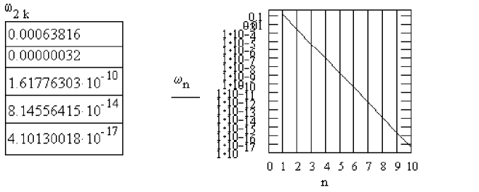
Figure 1: Numerical value of energy levels $\omega_{2k}$ and dependence of $\omega_{n}$ in the units of $\Upsilon$.

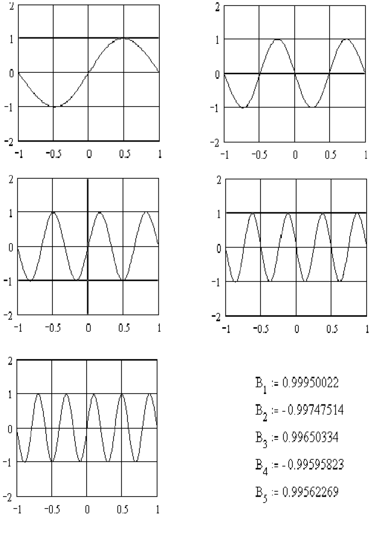
Figure 2: Solutions for $k=1,2,3,4,5$ and their Fourier-coefficients $B_{k}$.

References

- [1] H.Umezawa, H.Matsumoto and M.Tachiki, Thermo-Field Dynamics and Condensed States, North Holland Publishing Company, Amsterdam, 1982
- [2] A.M.Polyakov, Gauge Fields and Strings, Landau ITP, Chernogolovka, 1995 (in Russian)
- [3] S.P.Klevansky, Rev. Mod. Phys., 1992, 64, 649.
- [4] A.N. Vall, et.al. in D.V. Shirkov, D.I. Kazakov, A.A.Vladimirov, editors, Proceedings of X International Conference on Problems of Quantum Field Theory, JINR E2-96-369, 214, Dubna, 1996
- [5] A.N. Vall, et.al., Phys. Atom. Nucl., 1997, 60, 1314; Int. J. Mod. Phys. A, 1997, 12, 5039; Surveys in High Energy Physics, 1998, 13, 249.
- [6] K.A. Makarov, V.V. Melezhik, A.K. Motovilov, Theor. Math. Phys., 1995, 102, 258; K.A. Makarov, V.V. Melezhik,Theor. Math. Phys., 1996, 107, 415
- [7] F.A. Berezin, L.D. Faddeev, Dokl. Akad. Nauk SSSR, 1961, 137, 1011
- [8] C. Thorn, Phys. Rev. 1979, D19, 639
- [9] F.A. Berezin, Math.Collection, 1963, 60, 425
- [10] Yu.M. Shirokov, Theor. Math. Phys., 1980, 42, 45; ibid. 1981, 46, 291; ibid. 1981, 46, 310
- [11] Yu.G. Shondin, Theor. Math. Phys., 1982, 51, 181; ibid. 1985, 64, 432
- [12] C.J. Fewster, J.Phys.A: Math. Gen. 1995, 28, 1107
- [13] Yu.G. Shondin, Theor. Math. Phys., 1985, 65, 24; ibid. 1988, 74, 331
- [14] J.F. van Diejen, A. Tip, J.Math.Phys. 1991, 32(3), 630.
- [15] A.G. Sitenko, Lectures on Scattering Theory, ”Vischa Shkola”, 1971 (in Russian).
- [16] S. Albeverio, F. Gesztesy, R. Hoegh Krohn, H. Holden, Solvable Models in Quantum Mechanics, Springer-Verlag, 1988.
- [17] M. Reed, B. Simon, Methods of modern Mathematical Physics. 1. Functional analysis, Academic Press, 1972.
- [18] S.P. Merkuriev, L.D. Faddeev, Quantum Scattering Theory for Few-Body Systems, ”Nauka”, 1985 (in Russian).
- [19] M.V.Terentiev, Introduction to Theory of Elementary Particles, Moscow, ITEP, 1998 (in Russian).
- [20] R.M. Barnett at al., Review of Particle Properties, Phys. Rev., 1996, D54, 47.