Abstract

We present new analytic and numerical results for self-gravitating SU(2)-Higgs magnetic monopoles approaching the black hole threshold. Our investigation extends to large Higgs self-coupling, $\lambda$, a regime heretofore unexplored. When $\lambda$ is small, the critical solution where a horizon first appears is extremal Reissner-Nordstrom outside the horizon but has a nonsingular interior. When $\lambda$ is large, the critical solution is an extremal black hole with non-Abelian hair and a mass less than the extremal Reissner-Nordstrom value. The transition between these two regimes is reminiscent of a first-order phase transition. We analyze in detail the approach to these critical solutions as the Higgs expectation value is varied, and compare this analysis with the numerical results.

I Introduction

The physics of a nonsingular spacetime is qualitatively distinct from a that of a spacetime exhibiting a black hole. However, families of spacetimes exist that may be viewed as interpolating between the two. These spacetimes are nonsingular and have no horizons; nevertheless, they have a region whose metric can be made arbitrarily close to that of the exterior region of a black hole. In the limiting case, the inner boundary of this region takes on the characteristics of an extremal horizon, even though no curvature singularity develops in the interior. By studying such solutions, one may gain further insight into the properties of black holes.

One approach to the construction of such “almost black holes” begins with a spontaneously broken Yang-Mills theory that has magnetic monopole solutions. For small Higgs expectation values, these monopole solutions persist when gravitational effects are included. However, as the Higgs expectation value is increased toward a critical value on the order of the Planck mass, the monopole solutions begin to approximate black holes with finite mass and nonzero horizon radius.

Such gravitating monopoles, as well as the related magnetically charged black holes with hair, have been studied previously [1, 2, 3, 4, 5]. For a review article and recent work in related subjects, see [6]. In this paper we investigate these solutions in more detail, concentrating on some aspects that were not previously noted. Most notably, we find that two distinct types of behavior, with qualitatively different extremal black hole limits, can occur. Our focus here is on the detailed properties of these solutions and their behavior as they approach the black hole limit. We describe elsewhere [7] how these solutions can be used as approximate black holes that provide insight into the transition from a nonsingular spacetime to one with horizons.

We work in the context of an SU(2) gauge theory that is spontaneously broken to U(1) by a triplet Higgs field $\phi$ with vacuum expectation value $\langle\phi\rangle=v$. The elementary particle spectrum of this theory contains a pair of vector mesons $W^{\pm}$ that carry U(1) electric charge and have mass $ev$ (where $e$ is the gauge coupling), as well as a massless photon and a massive electrically neutral Higgs particle. In flat space the classical field equations have a spherically symmetric monopole solution with U(1) magnetic charge $4\pi/e$ and a mass of order $4\pi v/e$. This has a central “core” region, of radius $R_{\rm core}\sim 1/m_{W}$, in which there are nontrivial matter fields. Beyond this radius is a “Coulomb” region in which the massive fields fall off exponentially fast, leaving only a long-range Coulomb magnetic field.

In studying the behavior of these solutions in the presence of gravity, we assume spherical symmetry, and so can write the metric in the form

$$ds^{2}=B(r)dt^{2}-A(r)dr^{2}-r^{2}(d\theta^{2}+\sin^{2}\theta d\phi^{2})\ .$$ (1)

It is often convenient to rewrite $A$ in terms of a mass function $m(r)$ defined by

$${1\over A(r)}=1-{2Gm(r)\over r}$$ (2)

with $m(\infty)\equiv M$. For a configuration to be nonsingular at the origin, $A(0)=1$ and $m(0)=0$. A horizon occurs when $1/A$ has a zero or, equivalently, when $m(r)/r=1/2G$.

A benchmark with which to compare our results is provided by the Reissner-Nordstrom metric, with

$$B(r)={1\over A}=1-{2MG\over r}+{Q^{2}G\over 4\pi r^{2}}\ .$$ (3)

If $M>\sqrt{Q^{2}/4\pi G}$, this describes a black hole solution with a charge (either magnetic or electric) $Q$ and an outer horizon determined by the larger of the two zeroes of $1/A$. If instead $M<\sqrt{Q^{2}/4\pi G}$, there is no horizon separating the curvature singularity at $r=0$ from the asymptotic regions and a naked singularity results. The boundary between these two regimes, $M=\sqrt{Q^{2}/4\pi G}$, gives the extremal Reissner-Nordstrom black hole. For $Q=4\pi/e$, the case with which we will be concerned in this paper, the extremal black hole has a horizon radius

$$r_{0}=\sqrt{4\pi G\over e^{2}}$$ (4)

and a mass

$$M_{0}=\sqrt{4\pi\over Ge^{2}}\ .$$ (5)

When $v\ll M_{\rm Pl}$ the gravitational effects on the monopole are relatively small. The metric at large distances approaches the Reissner-Nordstrom form, with $\sqrt{Q^{2}/4\pi G}\gg M$. There is no singularity, because the actual metric deviates from the Reissner-Nordstrom form when $r\mathrel{\mathchoice{\lower 0.7pt\vbox{\halign{$\m@th\displaystyle\hfil#\hfil$\cr<\crcr\sim\crcr}}}{\lower 0.7pt\vbox{\halign{$\m@th\textstyle\hfil#\hfil$\cr<\crcr\sim\crcr}}}{\lower 0.7pt\vbox{\halign{$\m@th\scriptstyle\hfil#\hfil$\cr<\crcr\sim\crcr}}}{\lower 0.7pt\vbox{\halign{$\m@th\scriptscriptstyle\hfil#\hfil$\cr<\crcr\sim\crcr}}}}R_{\rm core}$. One finds that $1/A=1$ at the origin, decreases to a minimum at a radius of order $R_{\rm core}$, and then increases monotonically. As $v$ is increased, the core shrinks and the minimum of $1/A$ moves inward and becomes deeper. In most cases, this continues until $1/A$ develops a double zero, corresponding to an extremal horizon, when $v=v_{\rm cr}$. A slightly different behavior is found for very small Higgs self-coupling [3]. In this case, the solution varies continuously as $v$ is increased up to a value $v_{\rm max}$. Although the minimum value of $1/A$ is still nonzero at this point, static solutions do not exist for higher values of $v$. Instead, these solutions join smoothly on to a second branch of solutions for which $(1/A)_{\rm min}$ decreases as $v$ is decreased from $v_{\rm max}$ to a critical value $v_{\rm cr}$, where the extremal horizon develops.

For small values of the Higgs mass, the extremal horizon of the critical solution occurs at the Reissner-Nordstrom radius $r_{0}$, in the exterior Coulomb region of the monopole solution. The matter fields take on their vacuum value everywhere outside the horizon and the exterior metric is exactly that of an extremal Reissner-Nordstrom black hole. When the Higgs to vector mass ratio is greater than about 12, a regime not explored in depth in previous studies, the behavior is rather different. The horizon in the monopole core at a radius $r_{*}<r_{0}$ that decreases with increasing Higgs mass. In this case there are nontrivial matter fields, or “hair”, outside the horizon. The transition between the two regimes is not smooth, but instead is reminiscent of a first order transition.

The remainder of this paper is organized as follows. In Sec. II we outline the general formalism and define our conventions. In Sec. III we use numerical methods to obtain monopole solutions to the field equations. We describe in detail their behavior as $v$ is increased towards its critical value. The critical solutions that are the limits of these families of monopole solutions are characterized by the presence of extremal horizons. In Sec. IV, we use analytic methods to study the properties of these critical solutions, focusing on the behavior near the horizon. We show that the problem of finding a solution with an extremal horizon can be formulated as a pair of boundary value problems, one for the region $0<r<r_{*}$ and one for $r_{*}<r<\infty$, that must be solved simultaneously. The conditions for a solution to these places strong constraints on the behavior of the fields near the horizon. These constraints allow only two types of behavior, one associated with a core region horizon, the other with a Coulomb region horizon, which we examine in detail in Sec. V. In Sec. VI we compare these analytic predictions with our numerical results. Section VII contains some concluding remarks. The Appendix contains details of the numerical investigation of the transition region between the two types of critical solutions.

II General Formalism

We consider an SU(2) gauge theory with a triplet Higgs field $\phi^{a}$ whose self-interactions are governed by the scalar field potential

$$V(\phi)={\lambda\over 2}\left(\phi^{a}\phi^{a}-v^{2}\right)^{2}\ .$$ (6)

In flat spacetime, this theory has nonsingular monopole solutions, with magnetic charge $4\pi/e$, that are described by the spherically symmetric ansatz

$$\phi^{a} = v{\hat{r}}^{a}h(r)$$ (7)

$$A_{ia} = \epsilon_{iak}{\hat{r}}^{k}\,{1-u(r)\over er}$$ (8)

$$A_{0a} = 0\ .$$ (9)

While it is clear that $vh(r)$ is the magnitude of the Higgs field, the meaning of $u(r)$ is somewhat obscured by this “radial gauge” ansatz. By applying a singular gauge transformation that makes the direction of the Higgs field uniform, one finds that $u(r)/er$ is equal to the magnitude of the massive vector field, and so it, like $1-h(r)$, should be expected to vanish exponentially fast outside the monopole core.

The generalization of this ansatz to curved spacetime is straightforward. Since we are considering only static spherically symmetric solutions, we can take the metric to be of the form of Eq. (1). The matter part of the action is

$$S_{\rm matter}=-4\pi\int dt\,dr\,r^{2}\sqrt{AB}\left[{K(u,h)\over A}+U(u,h)\right]$$ (10)

where

$$K = \frac{1}{e^{2}r^{2}}\left(\frac{du}{dr}\right)^{2}+\frac{v^{2}}{2}\left(\frac{dh}{dr}\right)^{2}$$ (11)

$$U = {(u^{2}-1)^{2}\over 2e^{2}r^{4}}+{v^{2}u^{2}h^{2}\over r^{2}}+{\lambda v^{4}\over 2}(h^{2}-1)^{2}\ .$$ (12)

One may view $U(u,h)$ as a position-dependent potential. It has several stationary points, which we enumerate here for later reference:

1. $u=0$, $h=\pm 1$. This is a local minimum of $U$ for $r>1/ev$.

2. $u=\hat{u}(r)$, $h=\hat{h}(r)$, or $u=-\hat{u}(r)$, $h=-\hat{h}(r)$, where

   $$\hat{u} = \sqrt{\frac{\lambda(1-e^{2}v^{2}r^{2})}{\lambda-e^{2}}}$$ (13)

   $$\hat{h} = \sqrt{\frac{\lambda-e^{2}/(evr)^{2}}{\lambda-e^{2}}}\ .$$ (14)

   These are real only for $r$ lying between $1/ev$ and $1/\sqrt{\lambda}\,v$. In that range it is a minimum of $U$ if $\lambda/e^{2}>1$, but a saddle point if $\lambda/e^{2}<1$. If $\lambda/e^{2}=1$, this solution is replaced by a degenerate set of local minima, with $h^{2}+u^{2}=1$, that exist only for $evr=1$.

3. $u=h=0$. This is never a local minimum of $U$.

4. $u=\pm 1$, $h=0$. This is a local minimum of $U$ for $r<1/\sqrt{\lambda}\,v$.

We will see that these stationary points are key to understanding the local existence of extremal horizons in monopole systems.

For static solutions, the matter fields obey the equations

$${1\over\sqrt{AB}}\ \frac{d\ }{dr}\left(\frac{\sqrt{AB}}{A}\frac{du}{dr}\right) = \frac{e^{2}r^{2}}{2}\frac{\partial U}{\partial u}={u(u^{2}-1)\over r^{2}}+e^{2}v^{2}uh^{2}$$ (15)

$${1\over r^{2}\sqrt{AB}}\ \frac{d\ }{dr}\left(\frac{r^{2}\sqrt{AB}}{A}\frac{dh}{dr}\right) = {1\over v^{2}}\frac{\partial U}{\partial h}={2hu^{2}\over r^{2}}+2\lambda v^{2}h(h^{2}-1)\ .$$ (16)

These must be supplemented by the two gravitational field equations

$$\frac{1}{\sqrt{AB}}\frac{d\sqrt{AB}}{dr} = 8\pi GrK$$ (17)

$$r\ \frac{d\ }{dr}\left(\frac{1}{A}\right) = \left(1-8\pi Gr^{2}U\right)-\frac{1}{A}\left(1+8\pi Gr^{2}K\right)\ .$$ (18)

Note that, up to a rescaling of distances, the solutions of these equations depend only on the dimensionless parameters ${{a}}=8\pi Gv^{2}$ and ${{b}}=\lambda/e^{2}=(m_{H}/2m_{W})^{2}$.

Integration of Eq. (17) gives $B(r)$ in terms of the remaining functions. With the boundary condition $A(\infty)B(\infty)=1$, corresponding to the conventional normalization of $t$, we have

$$B(r)={1\over A(r)}\exp\left[-16\pi G\int_{r}^{\infty}dr^{\prime}\,r^{\prime}K\right]\ .$$ (19)

Using this result to eliminate $B(r)$ from the remaining field equations leaves one first-order and two second-order equations to be solved. A solution of these is determined by five boundary conditions. Requiring that the fields be nonsingular at the origin gives three of these, $u(0)=1$, $h(0)=0$, and $A(0)=1$. Two more, $u(\infty)=0$ and $h(\infty)=1$, follow from the finiteness of the energy. Additional boundary conditions arise when a horizon is present. While these are not relevant for our numerical solutions, which are all regular monopoles, they play an important role in our analysis of the extremal black hole configurations that are the limiting points of sequences of monopole solutions.

III Monopole Solutions

A The method

In our search for regular solutions and their approach to criticality, let us identify an energy functional on the space of static configurations. Following van Nieuwenhuizen, Wilkinson, and Perry [8], one can write down an action which is a functional of just $u(r)$ and $h(r)$ by not only eliminating $\sqrt{AB}$ using Eq. (17), but also eliminating $A$ by integrating Eq. (18) subject to the boundary condition $A(0)=1$. The complete action (i.e., gravitational plus matter) then becomes

$$S = -\int dt\ E$$ (20)

$$E = 4\pi\int_{0}^{\infty}dr\,\left\{\frac{r}{8\pi G}\frac{d\ }{dr}\sqrt{AB}\left[1-\frac{1}{A}\right]\right.$$ (22)

$$\ \ \ \ \ \ \ \ \ \ \ \ \ \ \ \ \ \ \ \ \ \ \ \left.+\ r^{2}\sqrt{AB}\left[{K(u,h)\over A}+U(u,h)\right]\right\}\ .$$

with $\sqrt{AB}$ and $A$ understood to be implicit functionals of $u(r)$ and $h(r)$. Configurations that extremize this action are solutions to Eqs. (15)-(18), with the energy $E$ being equal to the mass $M=m(\infty)$ [8]. This energy functional is not bounded from below, even when satisfying the appropriate boundary conditions, unless the $1/A(r)$ that corresponds to a given matter field configuration $\{u(r),h(r)\}$ is everywhere greater than zero. This restriction is not serious for our purposes, since we are only interested in static regular monopole solutions and their approach to criticality; all such solutions satisfy the condition that $1/A(r)>0$ everywhere.

Thus, we find regular solutions to the field equations by seeking extrema of this energy functional that satisfy the boundary conditions at $r=0$ and $r=\infty$. This is equivalent to solving $\delta E/\delta u=\delta E/\delta h=0$. We do this numerically by solving the alternative system of equations

$$\frac{d^{2}u}{dt^{2}}+\Gamma\frac{du}{dt}=\frac{\delta E}{\delta u}$$ (23)

$$\frac{d^{2}h}{dt^{2}}+\Gamma\frac{dh}{dt}=\frac{\delta E}{\delta h}$$ (24)

for an appropriate damping factor $\Gamma$ and taking the final steady state solution as the result. This approach is analogous to having a massive particle roll on a manifold determined by $E$ while the particle’s motion is viscously damped, eventually coming to rest at some local minimum of the energy.

The discretization used to numerically implement this algorithm places a limit on how close we can approach the critical solutions in which the extremal horizon has actually formed. The errors in the fields are proportional to the square of the spatial step size. As a result is that we can only obtain solutions in which the minimum value of $1/A$ is at least ${\cal O}[(\Delta r)^{2}]$.

One should contrast our relaxation method with the algorithms used in previous analyses [1, 2, 3] that employ shooting from the origin. In these, a choice is made for the values of the fields and their first spatial derivatives at the origin, and the equations of motion are then used to integrate out towards infinity. The initial choice is then adjusted to ensure that the boundary conditions at infinity are satisfied. With this approach, difficulties appear with large ${{b}}$ because of the extreme sensitivity at the origin to small perturbations. No such problem exists with relaxation, and as a result we have been able to obtain solutions for large ${{b}}$. However, although solutions that are unstable under perturbations may be found by shooting, such solutions cannot be obtained by our relaxation method.

In particular, previous work [3] has shown that for ${{b}}\mathrel{\mathchoice{\lower 0.7pt\vbox{\halign{$\m@th\displaystyle\hfil#\hfil$\cr<\crcr\sim\crcr}}}{\lower 0.7pt\vbox{\halign{$\m@th\textstyle\hfil#\hfil$\cr<\crcr\sim\crcr}}}{\lower 0.7pt\vbox{\halign{$\m@th\scriptstyle\hfil#\hfil$\cr<\crcr\sim\crcr}}}{\lower 0.7pt\vbox{\halign{$\m@th\scriptscriptstyle\hfil#\hfil$\cr<\crcr\sim\crcr}}}}0.1$ monopole solutions exist for a range of values of ${{a}}$ that are greater than the value ${{a}}_{\rm cr}$ of the critical solution. Moreover, for each value of ${{a}}$ in this range there are two solutions, with the one having the smaller value of $(1/A)_{\rm min}$ being unstable [9, 10]. Hence, for this range of $b$ our methods cannot find the critical limit of the regular monopole solutions.

B Approach to criticality: low–${{b}}$ case

We investigate the approach to criticality by studying the nature of the monopole solutions as ${{a}}=8\pi Gv^{2}$ is increased with the Higgs self-coupling held fixed. Two distinct behaviors are seen, depending on the size of ${{b}}=\lambda/e^{2}$.

FIG. 1.: Monopole solutions for ${{b}}=1.0$ and various values of $a$. The progression from dot-dashed line, to dashed line, to dotted line, to solid line corresponds to ${{a}}=1.0,2.0,2.3,$ and $2.37$. The first three panels depict the metric functions (a) $1/A(r)$, (b) $B(r)$, (c) $(AB)^{1/2}(r)$. (d) Matter fields variables; $u(r)$ begins at unity at the origin and asymptotes to zero as $r\rightarrow\infty$. $h(r)$ is zero at the origin and asymptotes to unity as $r\rightarrow\infty$.

We will describe the low-$b$ behavior in detail in this subsection, and the high-$b$ behavior in the next. Figure 1 illustrates the behavior for ${{b}}=1.0$, a typical low-$b$ case. As ${{a}}$ increases and gravitational effects become stronger, $1/A(r)$ begins to dip down until at ${{a}}={{a}}_{\rm cr}$ it develops a double zero, corresponding to an extremal horizon, at $r=r_{0}$, the horizon radius of the extremal Reissner-Nordstrom solution. At the same time, the matter fields $u(r)$ and $h(r)$ are pulled inward. At ${{a}}={{a}}_{\rm cr}$, the variation of these fields occurs entirely within the horizon. Only the Abelian Coulomb magnetic field survives outside the horizon, while the metric for $r\geq r_{0}$ is precisely that of the extremal Reissner-Nordstrom black hole.

All of this reproduces results found in earlier work [1, 2, 3, 4]. Some features that were not previously stressed are revealed when we examine $B(r)$. Coming in from large $r$, $B$ decreases with $1/A$ until the latter reaches its minimum. $B$ then continues to decrease, although at a much smaller rate. For very small ${{b}}$ this decrease continues all the way in to $r=0$, while for somewhat larger values of ${{b}}$ there is a minimum in $B$ at a finite $r<r_{0}$. The situation for the critical solution is somewhat ambiguous. If we adopt the conventional normalization $B(\infty)=1$, then $B(r)$ vanishes identically inside the horizon. If instead we set $B(0)=1$, then $B$ is finite and varying inside the horizon and infinite outside the horizon, with a minimum either at $r=0$ or at some finite radius, depending on the value of ${{b}}$. In neither case is the minimum a zero of $B$.

Closely related to this is the behavior of $\sqrt{AB}$. When ${{a}}$ is small, this is very nearly constant, with a value close to unity. As ${{a}}$ is increased, $\sqrt{AB}$ develops a step-like behavior until, at criticality, it is precisely a step function centered at the horizon. This is in sharp contrast with the Schwarzschild and Reissner-Nordstrom solutions, where $\sqrt{AB}=1$ everywhere. To show how this behavior becomes more pronounced as the solution approaches criticality, in Figure 2 we plot the value of $\sqrt{AB}$ at the origin as a function of $(1/A)_{\rm min}$ for ${{b}}=16$. Note that there is a power law relationship between the two. Similar curves, but with different powers, are found throughout the low-${{b}}$ regime.

FIG. 2.: $(AB)_{r=0}^{1/2}$ versus $(1/A)_{\rm min}$ for ${{b}}=16.0$ and various values of ${{a}}$ near ${{a}}_{\rm cr}$.

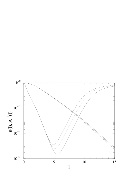
FIG. 3.: $A^{-1}$ (curves with minima) and $u$ (monotonic curves) as functions of the proper length $l$ for ${{b}}=16.0$. The progression from dashed line, to dotted line, to solid line corresponds to ${{a}}=1.529$, $1.53$ and $1.531$ with ${{a}}_{\rm cr}\approx 1.532$.

As a final illustration of the behavior of the low-${{b}}$ solutions near criticality, in Fig. 3 we plot $u$ for several near-critical solutions. However, rather than using the variable $r$, we have plotted $u$ as a function of the proper length

$$l(r)=\int_{0}^{r}dr\ \sqrt{A(r)}\,.$$ (25)

We see that, for sufficiently large $l$, $u(l)$ is close to a decaying exponential, and that this behavior does not significantly change as one crosses the minimum of $1/A$; similar behavior is seen with $1-h$.

C Approach to criticality: high–${{b}}$ case

The scenario when ${{b}}$ is large differs significantly from that for small ${{b}}$; we illustrate this in Fig. 4 for the case of ${{b}}=100$. So long as ${{a}}$ is not too near its critical value, the qualitative evolution of the metric functions and field variables is similar to that in the previous case: $1/A(r)$ dips down in a region $r\approx r_{0}$, the value of $B(r)$ decreases in a region near the origin, and the fields $u,h$ are drawn into the core of the system.

FIG. 4.: Monopole solutions for ${{b}}=100$ and various values of $a$. The progression from dot-dashed line, to dashed line, to dotted line, to solid line corresponds to ${{a}}=1.0$, 1.1, 1.2, and $1.29344$. The first three panels depict the metric functions (a) $1/A(r)$, (b) $B(r)$, (c) $(AB)^{1/2}(r)$. (d) Matter fields variables; $u(r)$ begins at unity at the origin and asymptotes to zero as $r\rightarrow\infty$. $h(r)$ is zero at the origin and asymptotes to unity as $r\rightarrow\infty$.

Near criticality, a different behavior emerges. The evolution of $1/A(r)$ as the solution approaches criticality is depicted in Fig. 4a and, in more detail, in Fig. 5. Although initially similar to that the for the low-${{b}}$ case, the decrease of the minimum at $r\approx r_{0}$ ceases before it actually reaches zero. As this occurs, a second minimum at a radius $r<r_{0}$ rapidly drops down and forms a double zero, corresponding to an extremal horizon, at $r=r_{*}<r_{0}$. Figure 4b (and, in more detail, Fig. 6) shows the function $B(r)$ as ${{a}}$ approaches its critical value. In contrast to the small-${{b}}$ case, in the critical limit the minimum of $B$ is a zero located at the horizon, $r=r_{*}$.

FIG. 5.: Details of the metric function $1/A(r)$ near criticality at ${{b}}=100$. The progression from dot-dashed line, to dashed line, to dotted line, to solid line corresponds to ${{a}}=1.27$, 1.29, 1.293, and $1.29344$.

FIG. 6.: Details of the metric function $B(r)$ near criticality at ${{b}}=100$. The progression for different ${{a}}$’s is the same as in Figure 5.

The evolution of $\sqrt{AB}$ is shown in Fig. 4c. The behavior is similar to that for the small-${{b}}$ case until the outer minimum of $1/A$ stops decreasing and the inner minimum begins to appear. Until this point, there is a power-law relationship between $\sqrt{AB}|_{r=0}$ and $(1/A)_{\rm min}$ similar to that for the small-${{b}}$ case, with most of the variation in $\sqrt{AB}$ occurring at $r\approx r_{0}$. Once the inner minimum begins to appear, the decrease in $\sqrt{AB}|_{r=0}$ slows down, so that even for the critical solution $\sqrt{AB}|_{r=0}\neq 0$.

Figure 4d depicts the matter fields $u(r)$ and $h(r)$ for a series of values of ${{a}}$ at fixed large ${{b}}$. Their behavior is analogous to that for small ${{b}}$ except that the fields are never completely drawn into the region $r<r_{0}$; the degree to which they are drawn into this region is dictated by the value of $1/A$ at the outer minimum at criticality. The smaller that minimum value of $1/A$, the more contained the matter fields are. Since they have nontrivial fields outside the horizon the critical solutions for large ${{b}}$ are examples of extremal black holes with non-Abelian hair.

FIG. 7.: Monopole solutions for ${{b}}=1000$ and various values of $a$. The progression from dot-dashed line, to dashed line, to dotted line, to solid line corresponds to ${{a}}=0.5$, 0.9, 1.0, and $1.05576$. The first three panels depict the metric functions (a) $1/A(r)$, (b) $B(r)$, (c) $(AB)^{1/2}(r)$. (d) Matter fields variables; $u(r)$ begins at unity at the origin and asymptotes to zero as $r\rightarrow\infty$. $h(r)$ is zero at the origin and asymptotes to unity as $r\rightarrow\infty$.

The qualitative picture differs somewhat when ${{b}}\mathrel{\mathchoice{\lower 0.7pt\vbox{\halign{$\m@th\displaystyle\hfil#\hfil$\cr>\crcr\sim\crcr}}}{\lower 0.7pt\vbox{\halign{$\m@th\textstyle\hfil#\hfil$\cr>\crcr\sim\crcr}}}{\lower 0.7pt\vbox{\halign{$\m@th\scriptstyle\hfil#\hfil$\cr>\crcr\sim\crcr}}}{\lower 0.7pt\vbox{\halign{$\m@th\scriptscriptstyle\hfil#\hfil$\cr>\crcr\sim\crcr}}}}400$, in that the $1/A$ always has only a single minimum. One may think of the sequence of monopole solutions here as large–${{b}}$ solutions in which the inner minimum of $1/A$ drops out sufficiently early that no double minimum solutions exist. To illustrate this, in Fig. 7 we show the approach to criticality for ${{b}}=1000$.

D Behavior of the critical solutions

The critical solutions themselves are not accessible through our numerical method. Nevertheless, we can obtain good approximations to these by following sequences of regular monopole solutions. Here we briefly summarize how some of the properties inferred from these numerical solutions vary with $b$.

FIG. 8.: Extremal horizon radius for various values of ${{b}}$. Analytic arguments indicate that $r_{*}\rightarrow 0$ as $b\rightarrow\infty$.

As we have already noted, the critical solutions for small $b$ have horizons at the Reissner-Nordstrom radius $r_{0}$, while for large $b$ the horizon occurs at a value $r_{*}<r_{0}$ (see Fig. 8). There is a discontinuity in passing from the low-$b$ to the high-$b$ regime: The critical solution does not continuously vary from one type to the other, but instead undergoes something like a first-order transition. For a value of $b$ just below the transition, an inner minimum appears at a radius $r<r_{0}$, while $1/A$ has a double zero at $r_{0}$. As $b$ increases, the inner minimum rapidly descends and at the transition $1/A$ has two degenerate minima, one at $r_{*}<r_{0}$ and the other at $r_{0}$. As $b$ increases further the outer minimum moves upward, while the inner minimum at $r_{*}$ remains at zero. Eventually the outer minimum vanishes, and the only minimum in $1/A$ is associated with the horizon at $r_{*}$. This radius $r_{*}$ asymptotes to zero as $b\rightarrow\infty$. As $b$ is increased, the critical black hole solution approaches that found in the literature in the infinite $b$ limit [3, 5].

FIG. 9.: Mass of critical solutions as a function of ${{b}}$. Low-${{b}}$ type solutions (${{b}}<40$) all have $M=M_{0}$. The dots indicate the values for high-$b$ type solutions.

The mass of the critical solution can be inferred from the long-range behavior of $1/A$. In Fig. 9 we plot this mass as a function of ${{b}}$. As expected, the mass of the low-${{b}}$ solutions is just that of an extremal Reissner-Nordstrom black hole. However, in the high-${{b}}$ regime the mass of the critical solution is less than the extremal Reissner-Nordstrom value $M_{0}$. The mass decreases with increasing ${{b}}$, and appears to have an asymptotic value of about 0.990. Note that there is no discontinuity in the mass in going from the low-$b$ to the high-$b$ regime.

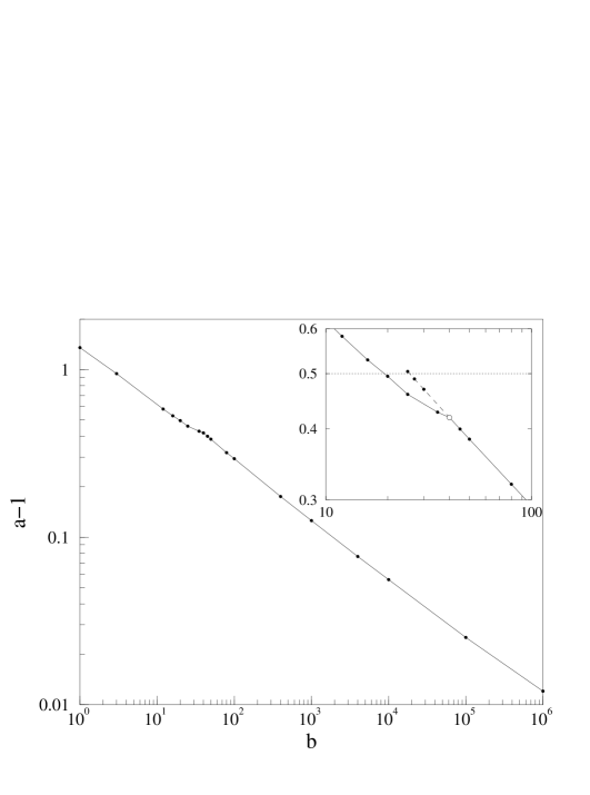
FIG. 10.: Critical values for ${{a}}-1$ as function of ${{b}}$. The inset shows in detail the transition region between low-${{b}}$ and high-${{b}}$ behavior, with the open circle indicating the apparent transition point at ${{b}}=40$. Note that at this point ${{a}}=1.4187<1.5$, the latter value indicated by the dotted line. The dashed line is an extension of the high-$b$ type critical solutions to smaller $b$. For the solutions represented by this dashed line, the fields are well-behaved inside the horizon, but are not asymptotically flat at spatial infinity.

Finally, Fig. 10 shows ${{a}}_{\rm cr}$ as a function of ${{b}}$. The critical value ${{a}}_{\rm cr}$ is always of order unity and is a monotonically decreasing function of ${{b}}$. This can be understood by recalling that the mass of the flat space monopole increases (by a factor of 1.8) as the ratio of the Higgs mass to the vector mass varies varies from zero to infinity. Stated differently, the value of $v$ needed to achieve a given mass decreases with increasing Higgs mass, making it plausible that the critical $v$ should decrease in a similar fashion.

For large ${{b}}$ there appears to be a power-law relationship between ${{b}}$ and ${{a}}_{\rm cr}-1$. That ${{a}}_{\rm cr}\rightarrow 1$ as $b\rightarrow\infty$ is consistent with observations made in past investigations [3, 4, 5]. The literature also [3] indicates that the curve should asymptote to ${{a}}_{\rm cr}\approx 3.94$ as ${{b}}\rightarrow 0$. The kink in the data at $b\approx 40$ is real and reflects the transition between the small and large ${{b}}$ regimes. Note that $a_{\rm cr}<1.5$ at this transition point; this fact will be of importance later. The dashed curve in the inset of Fig. 10 shows an extension of the high-$b$ type critical solutions into the low-$b$ regime. The corresponding solutions are well behaved inside the horizon, but are not asymptotically flat at spatial infinity; see the Appendix for more details.

IV Analytic constraints from extremal horizons

We would now like to use analytic methods to gain some deeper understanding of our numerical results. We begin by focusing on the critical solutions with extremal horizons, but regular at the origin, that are the limits of the gravitating monopole solutions. In this section we will obtain a set of conditions at the extremal horizon that are necessary, although not sufficient, for the existence of such solutions. These turn out to allow two distinct types of limiting solutions. We discuss both of these, as well as the nearby nearby nonsingular solutions, in more detail in the next section. Our analysis of the behavior of the fields near the horizon complements and extends earlier treatments [4, 11].

Because a simultaneous zero of both $1/A$ and its first derivative is a singular point of the differential Eqs. (15) and (16), the critical solutions are nonanalytic at the horizon radius $r_{*}$. Ordinarily, physical considerations would constrain the allowable singularities at such a point. However, we are not actually requiring that the solution be physically acceptable, but only that it be the limiting point of a family of physically acceptable solutions. Keeping this in mind, it seems reasonable to impose the following set of requirements:

1. We assume that the functions $u$, $h$, $1/A$, and $B$ are all finite and continuous at $r_{*}$.

2. Since $r$ is a singular coordinate at the horizon, we should not assume that the derivatives of these functions with respect to $r$ are continuous, or even finite, at $r_{*}$. Instead, we require only that $d(1/A)/dr$ vanishes at the horizon and that $du/dr$ and $dh/dr$ diverge less rapidly than $A^{1/2}$ does.

3. We assume that the leading singularities of these quantities near the horizon can be approximated by (not necessarily integer) powers of $|r-r_{*}|$, although we allow for the possibility that both the power and the coefficient of the leading term may be different on opposite sides of the horizon.

Given these assumptions, Eqs. (15) and (16) imply that the matter fields at the horizon, which we denote by $u_{*}$ and $h_{*}$, must lie at one of the stationary points of $U$ that were enumerated in Sec. II. Once these are specified, $r_{*}$ is determined by Eq. (18), which reduces to

$$0=1-8\pi Gr_{*}^{2}U(r_{*})\ .$$ (26)

The monopole solutions without horizons were solutions to a boundary value problem with conditions imposed at $r=0$ and $r=\infty$. The existence of the extremal horizon imposes three more conditions (on the values of $u$, $h$, and $1/A$ at $r=r_{*}$) and thus leads to a pair of boundary value problems, one for the interval $0\leq r\leq r_{*}$ and one for $r_{*}\leq r<\infty$, that must be solved simultaneously. The interior problem has three boundary conditions at the origin and three at the horizon, for a total of six, while the exterior has two at spatial infinity and three at the horizon, giving five in all.

A standard approach to such problems is to look for a family of solutions obeying the conditions at one of the boundaries. If these can be shown to depend on $N$ adjustable parameters, integration of these solutions will (assuming no singularities intervene) give an $N$-parameter family of solutions in the neighborhood of the other boundary. Generically, a necessary, although not sufficient, condition for a solution is that $N$ be greater than or equal to the number of conditions imposed at the second boundary. Thus, at first thought it would seem that, given a suitable set of values for $u_{*}$, $h_{*}$, and $r_{*}$, we would need a two-parameter family of solutions as $r-r_{*}\rightarrow 0_{+}$ to solve the exterior boundary value problem and a three-parameter family for $r-r_{*}\rightarrow 0_{-}$ to solve the interior problem. However, we do not expect to find extremal solutions for arbitrary values of parameters. Instead, for fixed ${{b}}$ we must adjust $v$ (or, equivalently, ${{a}}$) to its critical value. We may therefore view $v$ as an extra adjustable parameter, and need only require the existence of two-parameter families of solutions on both sides of the horizon. The nonanalyticity at the horizon allows us to choose the parameters on the two sides independently.

There are several caveats. First, the presence of the appropriate number of adjustable parameters at the horizon does not guarantee the existence of a solution. Global considerations that are beyond the scope of this analysis may make it impossible to satisfy all of the boundary conditions. Second, it may, and in some cases does, happen that the leading behavior near the horizon is fixed and that the adjustable parameters appear only in subdominant terms. Finally, if the values of $u$ and $h$ at the horizon are the same as at the origin (infinity), the interior (exterior) boundary value problem for the matter fields has a trivial solution, and so it is not necessary to have any adjustable parameters.

We find it convenient to define

$$\psi=\left(\matrix{u-u_{*}\cr\cr er_{*}v(h-h_{*})/\sqrt{2}}\right)$$ (27)

and to use the dimensionless position variable $x\equiv(r-r_{*})/r_{*}$. It is also useful to define the matrix

$${\cal M}_{ij}={e^{2}r_{*}^{4}\over 2}\left.{\partial^{2}U\over\partial\psi_{i}\partial\psi_{j}}\right|_{r_{*}}\ .$$ (28)

The orthonormal eigenvectors and the eigenvalues of ${\cal M}$ play an important role in the analysis; we denote these by $\theta_{a}$ and $\mu_{a}$ ($a=1$, 2), respectively. Finally, we define the two-component vector

$$\Phi_{i}={e^{2}r_{*}^{5}\over 2}\left.{\partial^{2}U\over\partial r\partial\psi_{i}}\right|_{r_{*}}$$ (29)

as well as the ratio

$$\sigma\equiv{4\pi G\over e^{2}r_{*}^{2}}={r_{0}^{2}\over r_{*}^{2}}$$ (30)

where, as before, $r_{0}$ is the horizon radius of the extremal Reissner-Nordstrom black hole.

Equation (18) and the equations obtained by substitution of Eq. (17) into Eqs. (15) and (16) form a set of three equations for the functions $u$, $h$, and $1/A$. In the notation we have just defined, the first two of these can be compactly written as

$${1\over A}\psi^{\prime\prime}+\left({1\over A}\right)^{\prime}\psi^{\prime}+{2\over A}\sigma[(\psi^{\prime})^{t}\psi^{\prime}]\psi^{\prime}={\cal M}\psi+\Phi x+\cdots$$ (31)

while the third becomes

$$\left({1\over A}\right)^{\prime}=2Fx-2\sigma\left[\psi^{t}{\cal M}\psi+{1\over A}(\psi^{\prime})^{t}\psi^{\prime}\right]+\cdots$$ (32)

where

$$F=-\sigma e^{2}r_{*}^{3}\left.{\partial(r^{2}U)\over\partial r}\right|_{r_{*}}\ .$$ (33)

Here primes denote derivatives with respect to $x$, while the ellipses represent terms, of higher order in either $x$ or the components of $\psi$, that can be neglected here.

We are assuming that the leading behavior of the various functions can be approximated by powers of $x$. It is then fairly easy to show that

$${1\over A}=kx^{2}+\cdots$$ (34)

This reduces Eqs.(31) and (32) to

$$k\left[x^{2}\psi^{\prime\prime}+2x\psi^{\prime}+2\sigma x^{2}[(\psi^{\prime})^{t}\psi^{\prime}]\psi^{\prime}\right]={\cal M}\psi+\Phi x+\cdots$$ (35)

and

$$k=F-\sigma\left[{1\over x}\psi^{t}{\cal M}\psi+kx(\psi^{\prime})^{t}\psi^{\prime}\right]+\cdots$$ (36)

We now turn to the behavior of $\psi$ as $x\rightarrow 0$. We see that $\psi$ must vanish at least as fast as $|x|^{1/2}$, since otherwise the nonlinear term on the left-hand side of the equation dominates and there is no solution. Hence, we may write

$$\psi=\eta_{1/2}|x|^{1/2}+\left[\eta_{1}x+\eta_{2}x^{2}+\cdots\right]+\eta_{\gamma_{1}}|x|^{\gamma_{1}}+\eta_{\gamma_{2}}|x|^{\gamma_{2}}+\cdots$$ (37)

where the ellipsis within the square brackets represents higher-order analytic terms, the $\gamma_{j}>1/2$ are noninteger powers to determined, and the final ellipsis represents smaller nonanalytic terms that are determined by the lower-order terms.

When this expansion is substituted into Eq. (35), the terms of order $|x|^{1/2}$ give the nonlinear equation

$$k\left[{3\over 4}-\epsilon{\sigma\over 4}\left(\eta_{1/2}^{t}\eta_{1/2}\right)\right]\eta_{1/2}={\cal M}\eta_{1/2}$$ (38)

where $\epsilon$ is equal to plus or minus unity according to whether $x$ is negative or positive (i.e., for the interior and exterior problems, respectively). A solution is possible only if $\eta_{1/2}$ is proportional to one of the eigenvectors of ${\cal M}$. Let us denote this eigenvector by $\theta_{\parallel}$ and the orthogonal eigenvector by $\theta_{\perp}$, with analogous conventions for the eigenvalues. We thus have

$$\eta_{1/2}=p\theta_{\parallel}$$ (39)

with $p$ obeying

$$kp\left[{3\over 4}-\epsilon{\sigma\over 4}p^{2}\right]=\mu_{\parallel}p\ .$$ (40)

In addition, substitution of our expansion for $\psi$ into Eq. (35) yields

$$k\left[1-\epsilon{\sigma\over 4}p^{2}\right]=F+\epsilon\sigma\mu_{\parallel}p^{2}\ .$$ (41)

These equations can be used to find $k$ as a function of $p^{2}$, and the result then substituted back into Eq. (40). For the interior solution ($\epsilon=1$), this leads to the result that

$$p^{2}_{\rm int}={F\over 2\sigma\mu_{\parallel}}\left[{4\mu_{\parallel}\over F}-1\pm\sqrt{1+{4\mu_{\parallel}\over F}}\right]\qquad\quad{\rm or}\qquad\quad p^{2}_{\rm int}=0$$ (42)

and

$$k_{\rm int}={4F\over(2-\sigma p_{\rm int}^{2})^{2}}\ .$$ (43)

Since $k$ must be positive, we require that $F>0$. The requirement that $p$ be real then implies that nonzero solutions for $p$ exist only if $\mu_{\parallel}\geq-F/4$; for the solution with the lower choice of sign, there is the additional requirement that $\mu_{\parallel}$ not lie between 0 and $3F/4$.

Although Eqs. (40) and (41) allow a nontrivial solution for $p^{2}$ in the exterior region, other constraints, described below, require that

$$p^{2}_{\rm ext}=0$$ (44)

and hence that

$$k_{\rm ext}=F\ .$$ (45)

Having determined $\eta_{1/2}$, we can now turn to the remaining terms in Eq. (37). Extracting the coefficients of the integral powers of $x$ in Eq. (35) yields a series of inhomogeneous linear equations that determine the $\eta_{n}$; the first of these is

$$(2k-{\cal M})\eta_{1}-\epsilon kp^{2}{\sigma\over 2}\left[2\left(\theta_{\parallel}^{t}\eta_{1}\right)\theta_{\parallel}+\eta_{1}\right]=\Phi\ .$$ (46)

In a similar fashion, the nonanalytic $O(|x|^{\gamma_{j}})$ terms give a linear equation for $\eta_{\gamma_{j}}$. However, because the inhomogeneous term in Eq. (35) is analytic and cannot contribute, the resulting equation is homogeneous. A solution of this equation is possible only if $\eta_{\gamma_{j}}$ is proportional to one of the $\theta_{a}$ and if $\gamma_{j}$ is a root of

$$0 = k\left[\gamma(\gamma+1)-{3\over 2}\epsilon\gamma\sigma p^{2}\right]-\mu_{\parallel}\,,\qquad\eta_{1/2}\propto\theta_{\parallel}$$ (47)

$$0 = k\left[\gamma(\gamma+1)-{1\over 2}\epsilon\gamma\sigma p^{2}\right]-\mu_{\perp}\,,\qquad\eta_{1/2}\propto\theta_{\perp}\ .$$ (48)

Note that both equations take the same form in the $p^{2}=0$ case, where the two $\mu_{a}$ are on the same footing. Because the equation is homogeneous, $\eta_{\gamma_{j}}$ is determined only up to an overall multiplicative constant. In order that the solution near the horizon have two adjustable constants, there must be two independent nonanalytic terms with powers greater than 1/2. Thus, the pair of equations corresponding to the two $\mu_{a}$ must, between them, have two roots greater than 1/2.

For $p=0$, the coefficient of $\gamma$ in Eq. (48) is positive, implying that at least one $\gamma$ must be negative for each $\mu_{a}$. In order to have two roots positive and greater than 1/2, we must require that both eigenvalues satisfy

$$\mu_{a}>{3F\over 4}>0\,,\qquad\qquad p=0\ .$$ (49)

For $p\neq 0$, the form of Eq. (48) depends on whether we are considering the mode proportional to $\theta_{\parallel}$ or the one proportional to $\theta_{\perp}$. In either case, it is most convenient to proceed by using Eq. (40) to eliminate $\mu_{a}$. For $\epsilon=-1$ the coefficient of $\gamma$ is positive, so at least one root is negative for each mode. Detailed examination of the equation for the $\theta_{\parallel}$ mode then shows that it has no roots greater than 1/2; since the equation for the $\theta_{\perp}$ mode can have at most one such, we must set $p=0$ in the exterior region. For $\epsilon=1$ (i.e., the interior region), the equation for the $\theta_{\parallel}$ mode has one and only root greater than 1/2 for all values of $\mu_{\parallel}$ consistent with the reality of $p$. The equation for the other mode can be rewritten as

$$0=\gamma\left(\gamma-{1\over 2}\right)+\left(\gamma-{1\over 2}\right)\left({2\mu_{\parallel}\over k}\right)+\left({\mu_{\parallel}-\mu_{\perp}\over k}\right)\ .$$ (50)

For this to have a solution with $\gamma>1/2$, either $\mu_{\parallel}<\mu_{\perp}$ or $\mu_{\parallel}<0$; since we will see that at most one of the $\mu_{a}$ can be negative, the second alternative implies the first. Combining this with the previous conditions on the $\mu_{a}$, we see that a $p\neq 0$ solution exists in the interior region if

$$\mu_{\perp}>\mu_{\parallel}>-{F\over 4}\,,\qquad\qquad p\neq 0\ .$$ (51)

Equations (49) and (51), together with the condition $F>0$, are the fundamental conditions that must be satisfied at the extremal horizon. To explore the various possibilities, we must apply these in turn to the stationary points of $U$ that were enumerated in Sec. II. The last two cases can be immediately eliminated: Case 3 is excluded because both $\mu_{a}<0$, thus ruling out the possibility of a $p=0$ exterior solution, while Case 4 has $F<0$. This leaves Cases 1 and 2. The former, $u_{*}=0$ and $h_{*}=1$, corresponds to an extremal horizon in the Coulomb region while the latter, $u_{*}=\hat{u}$ and $h_{*}=\hat{h}$, gives a horizon in the monopole core. We will study these in detail in the next section.

V Behavior near Coulomb and core region extremal horizons

In Sec. IV we showed that there are only two possibilities for the values of the fields at the extremal horizon. Although the local analysis that we used cannot tell whether these are consistent with the existence of a global solution, our numerical results show that both types of solution actually occur. In this section we examine these more closely. We also consider the nonsingular near-critical solutions in which $1/A$ has a related minimum.

A Coulomb region horizons

The first possibility, $u_{*}=0$, $h_{*}=1$, corresponds to a horizon in the Coulomb region outside the monopole core. Equation (26) implies that $r_{*}=r_{0}$, the extremal Reissner-Nordstrom value, so $\sigma=F=1$. The matrix ${\cal M}$ is diagonal, with eigenvalues

$$\mu_{1} = {\cal M}_{11}=(evr_{0})^{2}-1={{{a}}\over 2}-1$$ (52)

$$\mu_{2} = {\cal M}_{22}=4\lambda v^{2}r_{0}^{2}=2{{b}}{{a}}\ .$$ (53)

A solution outside the horizon is given by the extremal Reissner-Nordstrom metric, with $u=0$ and $h=1$ for all $r_{*}>r_{0}$. We assume that this is the only exterior solution satisfying the boundary conditions, and concentrate on the interior solution.

There are several possibilities for the behavior of fields just inside the horizon:

Type I: The singularity in the matter fields is less singular than $x^{1/2}$ (i.e., $p=0$). Equation (43) implies that $k=1$, so near the horizon

$$u = C_{u}|x|^{\gamma_{u}}+\alpha_{u}x+\cdots$$ (54)

$$h = 1-C_{h}|x|^{\gamma_{h}}-\alpha_{h}x+\cdots$$ (55)

$${1\over A} = x^{2}+\cdots$$ (56)

where the ellipses represent terms that are determined by the terms shown explicitly. Here $\alpha_{u}$ and $\alpha_{h}$ denote constants whose values are fixed by Eq. (46). $C_{u}$ and $C_{h}$ are not determined locally, but must instead be adjusted so the boundary conditions at the origin are satisfied. The exponents $\gamma_{u}$ and $\gamma_{h}$ are solutions of Eq. (48) and, depending on the values of ${{a}}$ and ${{b}}$, may or may not be greater than unity. The requirement that these exponents both be greater than 1/2 leads to Eq. (49), which implies that

$${{a}}>{\rm Max}\,\left[{7\over 2}\,,\,{3\over 8{{b}}}\right]\ .$$ (57)

Type II: Matter fields with $|x|^{1/2}$ singularities. There are two possibilities here, depending on which field has the singularity. In the first (Type IIa),

$$u = p|x|^{1/2}+C_{u}|x|^{\gamma_{u}}+\alpha_{u}x+\cdots$$ (58)

$$h = 1-C_{h}|x|^{\gamma_{h}}-\alpha_{h}x+\cdots$$ (59)

$${1\over A} = kx^{2}+\cdots$$ (60)

while in the second (Type IIb),

$$u = C_{u}|x|^{\gamma_{u}}+\alpha_{u}x+\cdots$$ (61)

$$h = 1-p\sqrt{{{a}}}|x|^{1/2}-C_{h}|x|^{\gamma_{h}}-\alpha_{h}x+\cdots$$ (62)

$${1\over A} = kx^{2}+\cdots$$ (63)

Here

$$k=(1-p^{2}/2)^{-2}$$ (64)

and

$$p^{2}={1\over 2\mu_{\parallel}}\left[4\mu_{\parallel}-1\pm\sqrt{1+4\mu_{\parallel}}\right]$$ (65)

with $\mu_{\parallel}$ equal to the lesser of the two eigenvalues in Eq. (53). If $2<{{a}}<7/2$, the upper sign must be used in Eq. (65). For Type IIa solutions Eq. (51) requires that either

$${3\over 2}<{{a}}<{2\over 1-4{{b}}}\qquad{\rm and}\quad{{b}}<{1\over 4}$$ (66)

or

$${{a}}>{3\over 2}\qquad{\rm and}\quad{{b}}>{1\over 4}\ .$$ (67)

The corresponding requirement for Type IIb is that

$${{a}}>{2\over 1-4{{b}}}>2\qquad{\rm and}\quad{{b}}<{1\over 4}\ .$$ (68)

At the boundary between the IIa and IIb regimes, ${{a}}=2/(1-4{{b}})$, both $\gamma_{u}$ and $\gamma_{h}$ are equal to 1/2 and the two types of solutions merge. Note that none of these solutions is possible if ${{a}}<3/2$; this point will be important when we compare this analysis to the numerical results.

The most important difference between the Type I and the Type II solutions is in the behavior of the quantity $\sqrt{AB}$. If $p\neq 0$, one of the matter fields varies as $|x|^{1/2}$ near the horizon. As a result, the integral in the exponent in Eq. (19) diverges for any $r<r_{0}$, and $\sqrt{AB}$ becomes a step function centered at the horizon. Horowitz and Ross [12] have shown that a particle in geodesic motion across a horizon feels a tidal force proportional to the logarithmic derivative of $\sqrt{AB}$, and have used the term “naked black holes” to describe certain near-extremal black holes solutions for which this quantity is large. Not only do our Coulomb region extremal solutions fit in this category, but so do the nearby nonsingular solutions.

B Horizons in the monopole core

The second possibility allowed by the analysis of Sec. IV is that $u_{*}=\hat{u}(r_{*})$ and $h_{*}=\hat{h}(r_{*})$, with $\hat{u}$ and $\hat{h}$ given by Eqs. (13) and (14). This corresponds to a horizon in the monopole core region. Unlike the case of a Coulomb region horizon, there must be a nontrivial exterior solution, thus giving an extremal black hole with Higgs and gauge boson hair. Because our numerical results show solutions of this type only for relatively large values of ${{b}}$, we will find it convenient to use large-${{b}}$ expansions to simplify some of the algebra below.

Substituting the expressions for $\hat{u}$ and $\hat{h}$ into the potential $U$ gives

$$8\pi Gr^{2}U={{{a}}\over 2({{b}}-1)}(evr)^{-2}\left[-1+2{{b}}(evr)^{2}-{{b}}(evr)^{4}\right]\ .$$ (69)

Equation (26) requires that this be equal to unity at the horizon. By making use of the fact that $(evr_{*})^{2}={{a}}/2\sigma$, this constraint can be rewritten as

$${{b}}={4\sigma(1-\sigma)\over{{a}}^{2}-4{{a}}\sigma+4\sigma}\ .$$ (70)

The roots of this equation determine ${{a}}$ in terms of ${{b}}$ and $\sigma$. For large ${{b}}$, the ${{b}}$-dependence is negligible, and

$${{a}}=2\sigma\left[1\mp\sqrt{1-\sigma^{-1}}\right]+O(1/{{b}})\ .$$ (71)

In contrast with the previous case, the matrix ${\cal M}$ is not diagonal. Using the equations obeyed by $\hat{u}$ and $\hat{h}$, it can be written as

$${\cal M} = \left(\matrix{2{\hat{u}}^{2}&2\sqrt{2}evr_{*}\,\hat{u}\hat{h}\cr\cr 2\sqrt{2}evr_{*}\,\hat{u}\hat{h}&4{{b}}e^{2}v^{2}r^{2}_{*}\,{\hat{h}}^{2}}\right)$$ (72)

$$= \left(\matrix{2(1-y^{2})&2\sqrt{2}y\sqrt{1-y^{2}}\cr\cr 2\sqrt{2}y\sqrt{1-y^{2}}&4{{b}}y^{2}-4(1-y^{2})}\right)+O(1/{{b}})$$ (74)

where in the second line we have defined

$$y^{2}=(evr_{*})^{2}={{{a}}\over 2\sigma}\ .$$ (75)

The eigenvalues of ${\cal M}$ are

$$\mu_{1} = {2{{b}}{{a}}\over\sigma}+O(1)$$ (76)

$$\mu_{2} = 2-{{{a}}\over\sigma}+O(1/{{b}})\ .$$ (78)

The exterior solution must be of the $p=0$ type, implying that these eigenvalues must obey Eq. (49). This requires that they both be greater than $3F/4$, where

$$F = {1\over{{b}}-1}\left[{{{a}}^{2}{{b}}\over 4\sigma}-\sigma\right]$$ (79)

$$= {{{a}}^{2}\over 4\sigma}+O(1/{{b}})\ .$$ (80)

In the large ${{b}}$ limit, $\mu_{1}$ clearly satisfies this condition, while for $\mu_{2}$ we obtain the constraint

$$\sigma>{3\over 32}{{a}}^{2}+{1\over 2}{{a}}+O(1/{{b}})\ .$$ (81)

We also obtain the requirement ${{b}}>1$, since otherwise $M$ has a negative eigenvalue. Since ${{a}}$ and $\sigma$ are also related by Eq. (71), we can obtain a constraint that depends only on $\sigma$. To satisfy both Eqs. (71) and (81), we must take the upper sign in Eq. (71). We can then combine the two conditions to obtain

$$6\sigma^{2}-{41\over 15}\sigma-4+O(1/{{b}})>0$$ (82)

which implies that $\sigma>1.06+O(1/{{b}})$. Note in particular that $\sigma=1$ (i.e., $r_{*}=r_{0}$) is not possible for any value of ${{b}}$.

Once this condition is satisfied, there are no further constraints imposed by local analysis at the horizon. In particular, the interior solution can be either of the $p=0$ or the $p\neq 0$ type. Because ${\cal M}$ is not diagonal, as it was in the Coulomb case, the same irrational powers appear in both $u$ and $h$. Thus, if $p=0$, the fields near the horizon behave as

$$u = \hat{u}(r_{*})+q_{1}^{u}C_{1}|x|^{\gamma_{1}}+q_{2}^{u}C_{2}|x|^{\gamma_{2}}+\alpha_{u}x+\cdots$$ (83)

$$h = \hat{h}(r_{*})+q_{1}^{h}C_{1}|x|^{\gamma_{1}}+q_{2}^{h}C_{2}|x|^{\gamma_{2}}+\alpha_{h}x+\cdots$$ (84)

$${1\over A} = Fx^{2}+\cdots$$ (85)

Here $\gamma_{1}$ and $\gamma_{2}$ are solutions of Eq. (48) corresponding to the two $\mu_{a}$; as before, their values may be either greater or less than unity, depending on the values of ${{a}}$ and ${{b}}$. The constants $q_{a}^{u}$ and $q_{a}^{h}$ are determined by the eigenvectors $\theta_{a}$. The values of $\alpha_{u}$ and $\alpha_{h}$ are fixed and are the same on both sides of the horizon, while $C_{1}$ and $C_{2}$ can be varied independently inside and outside the horizon so that the boundary conditions can be satisfied both at the origin and at spatial infinity.

If instead $p\neq 0$, the fields outside the horizon are as in Eq. (85), but inside the horizon

$$u = \hat{u}(r_{*})+pq_{2}^{u}|x|^{1/2}+q_{1}^{u}C_{1}|x|^{\gamma_{1}}+q_{2}^{u}C_{2}|x|^{\gamma_{2}}+\alpha_{u}x+\cdots$$ (86)

$$h = \hat{h}(r_{*})+pq_{2}^{h}|x|^{1/2}+q_{1}^{h}C_{1}|x|^{\gamma_{1}}+q_{2}^{h}C_{2}|x|^{\gamma_{2}}+\alpha_{h}x+\cdots$$ (87)

$${1\over A} = kx^{2}+\cdots$$ (88)

We have assumed that $\mu_{2}<\mu_{1}$; if the opposite were the case, the $|x|^{1/2}$ terms would involve $q_{1}^{u}$ and $q_{1}^{h}$. Here $k$ and $p$ are given by Eqs. (43) and (42), with there being two acceptable solutions. As before, the values of $\alpha_{u}$ and $\alpha_{h}$ are determined, although they are no longer the same as in the external solution.

VI Comparison with numerical results

Let us now see how well these analytic results agree with our numerical results. We begin with the low-${{b}}$ regime, where the nonsingular monopole solutions tend toward a critical solution with a Coulomb region horizon at the Reissner-Nordstrom value $r=r_{0}$. Throughout this regime, the critical solutions we find appear to be the more singular Type II solutions rather than the Type I solutions of Eq. (56). This is consistent with our finding (see Fig. 10) that the values of ${{a_{\rm cr}}}$ are always less than the lower bound for Type I solutions given in Eq. (57).

Given the values for ${{a_{\rm cr}}}$ as a function of ${{b}}$, Eqs. (66) and (68) predict that there should be a transition at ${{b}}\approx 0.1$ between the Type IIa regime, where $u\sim|x|^{1/2}$ and the Type IIb regime, where $1-h$ has the $|x|^{1/2}$ singularity. At ${{b}}=0.1$, the lowest ${{b}}$ for which we have a sequence of stable configurations that approaches a critical black hole solution, we find that the powers of $u$ and $1-h$ are both close to $1/2$, as predicted for this transition. It is curious to note that this is close to the value of ${{b}}$ below which $(1/A)_{\rm min}$ can be a double-valued function ${{a}}$.

Examining the Coulomb-type black hole solutions in more detail, we find, for ${{b}}\mathrel{\mathchoice{\lower 0.7pt\vbox{\halign{$\m@th\displaystyle\hfil#\hfil$\cr<\crcr\sim\crcr}}}{\lower 0.7pt\vbox{\halign{$\m@th\textstyle\hfil#\hfil$\cr<\crcr\sim\crcr}}}{\lower 0.7pt\vbox{\halign{$\m@th\scriptstyle\hfil#\hfil$\cr<\crcr\sim\crcr}}}{\lower 0.7pt\vbox{\halign{$\m@th\scriptscriptstyle\hfil#\hfil$\cr<\crcr\sim\crcr}}}}20$, that as $r$ approaches $r_{0}$ from below, the values of $d^{2}(A^{-1})/dx^{2}$ and $u^{2}/x$ tend toward the values of $k$ and $p$ predicted by Eqs. (64) and (65) with the upper choice of sign.

We observed in Sec. IIIB that the matter fields displayed exponential falloffs when written as functions of the proper length $l(r)$ for low-${{b}}$ type solutions. To understand this, we note that the field equation for $u$, Eq. (15), can be written as

$${d^{2}u\over dl^{2}}+\left[{d(A^{-1/2})\over dr}+{8\pi GrK\over\sqrt{A}}\right]{du\over dl}={u(u^{2}-1)\over r^{2}}+e^{2}v^{2}uh^{2}\ .$$ (89)

Our analytic results indicate that the quantity in square brackets is of order unity as $x\rightarrow 0$ for the interior portion of the extremal solution. This suggests that this quantity should be a relatively slowly varying function for large $l$ and hence that the falloff of $u$ should behave as a decaying exponential with a slowly-varying decay constant. As we saw in Fig. 3, this is indeed the case both for the critical and the near-critical solutions. A similar analysis can be applied to $1-h$.

From this point of view, the vanishing of $u$ and $1-h$ at the extremal horizon is a simple consequence of the fact that $l(r_{0})=\infty$. This analysis also tells us how these fields should behave as the critical solution is approached. We concentrate here on $u$, and restrict ourselves to the range of ${{b}}$ where $u\sim|x|^{1/2}$ in the critical solution. Near $\bar{r}$, the minimum of $1/A$, we can write

$${1\over A}\approx c_{1}^{2}(r-\bar{r})^{2}+\Delta^{2}\ .$$ (90)

Substituting this into Eq. (25), we find that

$$\bar{l}\equiv l(\bar{r})\sim c_{1}^{-1}\ln(1/\Delta)\ .$$ (91)

Writing $u$ as a decreasing exponential, $u\sim u_{0}\exp(-c_{2}l)$, we then have

$$u(\bar{r})\sim u_{0}(1/A)_{\rm min}^{q}$$ (92)

with $q=c_{2}/2c_{1}$. This analysis does not give predictions for $c_{1}$ and $c_{2}$. However, we can get an indication of what to expect for $q$ by recalling that for the critical ($\Delta=0$) case $u\sim(1/A)^{1/4}$ as the horizon is approached from the inside. If the above expressions were exact and $c_{1}$ and $c_{2}$ were truly constant and independent of $\Delta$, this would imply that $q=1/4$. Turning to our numerical results, we do indeed see a power law behavior for $u$, with $q$ ranging between 0.23 and 0.28.

A similar analysis can be applied to the jump in $\sqrt{AB}$ near the minimum of $1/A$. For the parameter ranges where we find extremal solutions with $p\neq 0$, this predicts that $\sqrt{AB}_{\rm r=0}$ varies as $(1/A)_{\rm min}^{-p^{2}/4}$ assuming a normalization of $\sqrt{AB}_{\rm r=\infty}=1$. Not only does this account for the power law behavior noted in Sec. IIIB, but the predictions for the power are borne out by the data within the numerical accuracy, where the power $p^{2}/4$ ranges from about 0.7 to unity.

Near ${{b}}=20$, ${{a}}_{\rm cr}$ equals $3/2$, the lower bound allowed by the analysis of the previous section for Coulomb-type solution. Nevertheless, the qualitative nature of the approach to criticality does not change as ${{b}}$ increases past this value and as ${{a}}_{\rm cr}$ becomes smaller than $3/2$. Indeed, the transition to core-type horizons does not appear to occur until about ${{b}}=40$, where ${{a}}_{\rm cr}=1.4187$. It does not seem as if this discrepancy can be attributed simply to numerical errors. We find that changing numerical parameters or modifying details of the algorithm gives a variation in the value of $a_{\rm cr}$ at the transition that is at most of order 0.01. For more details of the numerical aspect of this issue, see the Appendix.

The resolution of this puzzle seems to lie beyond the precision of our numerical simulations. Several possibilities suggest themselves. First, there may be a sharp change in the approach to criticality that is only seen when one reaches solutions for which $(1/A)_{\rm min}$ is less than the limits set by our spatial step size, in such a way that our extrapolation to the critical limit is incorrect. It could be that the decrease in the minimum of $1/A$ suddenly slows, and that it only reaches zero at ${{a}}_{\rm cr}>3/2$, or it could be that a new family of solutions intervenes. Alternatively, it may be that ${{a}}_{\rm cr}$ is correctly extrapolated, but that the critical solution violates one or more of the assumptions that we enumerated at the beginning of Sec. IV. For example, the critical solution might have discontinuities in the matter fields at the horizon; because this would occur at a zero in $1/A$, it would not necessarily lead to a divergent energy.

We turn now to the high-${{b}}$ regime, where the critical solution has an extremal horizon in the core region, with $u_{*}=\hat{u}(r_{*})$, $h_{*}=\hat{h}(r_{*})$. The numerical solutions all have $p=0$ for both the internal and external solutions, with the matter fields varying less rapidly than $|x|^{1/2}$ near the horizon. Moreover, for the entire region where we observe this type of black hole solution, the leading behavior of $u-u_{*}$ and $h-h_{*}$ at the horizon appears to be linear in $x$, with the nonanalytic terms being subdominant. The relations between ${{a}}$, $u_{*}$, $h_{*}$ and $r_{*}$ are all in agreement with our analytic results.

Examining the solutions in more detail, we find that in most of the interior portion of the critical and near-critical solutions both $u(r)$ and $h(r)$ closely track $\hat{u}(r)$ and $\hat{h}(r)$. This is easily understood by recalling the form of the matter action, Eq. (10). Once $1/A$ has become small, the gradient terms in the action are much less important than the position-dependent potential $U$. As a result, the fields that minimize the action should point-by-point be close to the minimum of $U$, namely $\hat{u}(r)$ and $\hat{h}(r)$.

It may be at first surprising that a second minimum in $1/A$ exists at $r\approx r_{0}$ outside the true horizon. To explain this, consider the behavior of the metric outside the monopole core. If the matter fields $u$ and $h$ are negligibly small for $r>R_{\rm core}$, then in this Coulomb region the mass function for a configuration with magnetic charge $4\pi/e$ can be approximated by

$$m(r)=M-{2\pi\over e^{2}}\ .$$ (93)

This gives a local maximum of $m(r)/r$, corresponding to a local minimum of $1/A$, at

$$r_{\rm min}={4\pi\over e^{2}M}=r_{0}\left({M_{0}\over M}\right)$$ (94)

with the value of $1/A$ at this minimum being $1-(M/M_{0})^{2}$. This minimum will occur, regardless of whether or not there is a horizon at a smaller value of $r$, as long as $r_{\rm min}>R_{\rm core}$. It is absent in our solutions for very large ${{b}}$ because for those solutions ${{a}}$, and thus $v$, are small enough that the core extends beyond $r_{0}$.

VII Concluding Remarks

We have used both analytic and numerical methods to study self-gravitating Yang-Mills-Higgs magnetic monopoles for a range of parameters, with an emphasis on their approach to the black hole threshold as the Higgs expectation value tends toward its critical value. We find two quite distinct behaviors. In the low-$b$ regime, with weak Higgs self-coupling, the critical solution is identical to the extremal Reissner-Nordstrom solution outside the horizon. Inside the horizon, the matter fields are smooth and nonsingular, as is $1/A$. However, because of the step function behavior of $\sqrt{AB}$ at the horizon, $B=g_{tt}$ vanishes identically in the interior. The associated singularity at the horizon means that an observer falling freely into a critical or near-critical monopole will experience the strong tidal forces characteristic of a Horowitz-Ross naked black hole.

One might speculate that these singularities were inextricably associated with the transition from a nonsingular monopole to a black hole spacetime and were independent of the details of the Higgs potential. However, our solutions in the large-$b$ regime show that this is not the case. For these, the critical solution has nontrivial matter fields outside the horizon, and thus is an extremal black hole with hair. Although the metric functions are still nonanalytic at the horizon, their singularities are much weaker and do not lead to large tidal forces.

The transition between these two regimes is itself quite interesting, and is in many ways reminiscent of a first-order transition. For a range of values of $b$ on both sides of the transition point, $1/A$ for the critical solution has two distinct minima. For values of $b$ below the transition, $1/A$ is positive at the inner minimum and has a double zero at the outer minimum at $r=r_{0}$. The inner minimum moves downward with increasing $b$ until, at the transition point, there are two distinct but degenerate minima, with $1/A$ vanishing at both. As $b$ is increased further, the outer minimum moves upward while the inner minimum remains a zero of $1/A$. While this implies a discontinuity in the horizon area, the mass of the black hole is continuous. In terms of black hole thermodynamics, this corresponds to a discontinuity in the entropy but (because these are zero temperature black holes) a free energy that is a continuous function of $b$.

Our focus in this paper has been on the behavior of the monopole solutions as the Higgs expectation value is increased to its critical value. It seems natural to ask how these solutions evolve if $v$ is increased still further. Actually, there is a bifurcation at this point. If one requires that the solutions remain well-behaved at spatial infinity, the solutions with $v>v_{\rm cr}$ are black hole solutions with singularities at $r=0$. In the low-$b$ regime, these are simply nonextremal Reissner-Nordstrom black holes, of varying mass, with no dependence on either $a$ or $b$. (There are also magnetically-charged black holes with hair in this regime; however, they are not continuously connected to our critical solutions.) In the high-$b$ regime, the counting of boundary conditions suggests that, for given values of $a$ and $b$, the continuation of the external solution is a one-parameter family of black holes with hair. Alternatively, one can require that the fields remain nonsingular at $r=0$ and continue the interior solution. Because there are three boundary conditions at the origin, compared to the two at spatial infinity, this gives solutions with nonsingular interiors bounded by horizons that are uniquely determined by specifying $a$ and $b$. The behavior of the metric near the horizon is similar to that found when de Sitter spacetime is written in static coordinates, suggesting a cosmological interpretation for these solutions. We suspect that, possibly with a suitably modified Higgs potential, these may give rise to topological inflation [13, 14].

Finally, having studied these self-gravitating monopoles and obtained an understanding of their approach to criticality, we can use these solutions as tools for investigating the transition from a nonsingular spacetime to one containing blackhole horizons. We will describe this elsewhere.

A Numerical Discussion of Transition Regime

In Section VI we noted that a discrepancy appears between the analytic argument that low-$b$ type critical solutions can only exist when $a_{\rm cr}>1.5$ and the numerical observation that this type of critical solution persists when $a_{\rm cr}<1.5$. We discuss here the details of our investigation that lead us to believe that this discrepancy is not a numerical artifact.

Recall that the transition between the high and low-$b$ type critical solutions is reminiscent of a first-order phase transition. The metric function $1/A(r)$ for a regular monopole solution near criticality with $b$ near the transition value possesses two minima, one near the extremal Reissner-Nordstrom radius, $r_{0}$, the other in the core of the monopole, $r<r_{0}$. As $a$ is increased (for a fixed $b$), one of these minima becomes a horizon, and a critical solution is attained. If $1/A$ at the inner minimum becomes zero first, then we have a high-$b$ type critical solution; when $1/A$ for the outer minimum touches down first, we have low-$b$ type solution. Let us examine each of these minima separately for regular solutions near criticality in this transition region.

1 The core minimum

The inner minimum for the types of solutions under consideration varies rapidly with both $a$ and $b$, so one can identify very precisely when such a minimum becomes a horizon. Moreover, the field variables and their derivatives are well-behaved near this radius, and the numerical solutions here are robust and insensitive to variations in the numerical algorithm. Different numerical implementations of the field equations leads to differences in $a_{\rm cr}$ of a few parts in $10^{4}$ for a high-$b$ type critical solution.

The numerical and analytic results could be reconciled if (1) the high-$b$ type solutions persisted down to lower $b$ into a region where $a_{\rm cr}>1.5$ and (2) the identification of the outer minimum as a zero of $1/A$ for the critical solutions in this region was a result of numerical error. We can address the first issue by using a trick. In Sec. IV we learned that critical solutions solve separate interior and exterior boundary value problems. Hence, we can determine $a_{\rm cr}$ as a function of $b$ for the high-$b$ type solutions by just solving the field equations from the origin to the horizon, ignoring the exterior region from the horizon out to spatial infinity. By using an algorithm similar to that described in Sec. III, we find the family of critical solutions represented by the dashed line in the inset of Figure 10. These solutions have high-$b$ type horizons but are not asymptotically flat at spatial infinity; however, if there were an asymptotically flat critical solution with the same value of $b$, it would have the same $a_{\rm cr}$ as these solutions. This dashed line crosses $a_{\rm cr}=1.5$ when $b=25.6$. Thus to be consistent with the analytic results, the transition value between low and high-$b$ critical solutions must occur for $b<25.6$ (rather that at the value of $b=40$ indicated by our numerical results). Again, this result appears to be numerically robust to a few parts in $10^{4}$.

2 The Coulomb minimum

According to the previous discussion, the ability to reconcile numerical and analytic results now depends on the sensitivity of the outer minimum, the one near $r_{0}$, to numerical error. From the inset in Figure 10, we see that in order for $b_{\rm tr}<25.6$, our values for $a_{\rm cr}$ for the low-$b$ type critical solutions must be in error (too low) by approximately $0.04$. A priori, such an error is certainly plausible. At this minimum, the solutions near criticality vary sluggishly with $a$ and $b$. The spatial derivatives of field variables are large at this radius, and indeed are expected to be singular if the outer minimum becomes a horizon. It is here that we are most susceptible to numerical errors.

As we discussed in Sec. III, discretized versions of Eqs. (15)–(18) are implemented in our numerical algorithm to identify static monopole solutions. In order to probe the robustness of the algorithm and the confidence with which we can treat these solutions, different implementations of the discretization were examined and compared. In particular, we focus on Eqs. (15) and (16). First, we used the straightforward expansion of these equations.

$${1\over A}{d^{2}u\over dr^{2}} + {du\over dr}\left[{d\over dr}\left({1\over A}\right)+8\pi G{rK\over A}\right]=\cdots$$ (A1)

$${1\over A}{d^{2}h\over dr^{2}} + {dh\over dr}\left[{d\over dr}\left({1\over A}\right)+8\pi G{rK\over A}+{2r\over A}\right]=\cdots\ .$$ (A2)

In a separate treatment, we used Eq. (18) to eliminate $d(1/A)/dr$.

$${1\over A}{d^{2}u\over dr^{2}}+{1\over r}{du\over dr}\left[(1-8\pi Gr^{2}U)-{1\over A}\right] = \cdots$$ (A3)

$${1\over A}{d^{2}h\over dr^{2}}+{1\over r}{dh\over dr}\left[(1-8\pi Gr^{2}U)+{1\over A}\right] = \cdots\ .$$ (A4)

Though these two systems of equations are equivalent in the continuum limit, their discretized forms which appear in the numerical implementation suffer a ${\cal O}[(\Delta r)^{2}]$ difference.

Figure 11 shows the $(1/A)_{\rm min}$ as a function of $a$ for solutions near criticality using the two different equation sets Eq. (A1) and (A3) at $b=16$ and $b=35$. The curves in Fig. 11 do not extend into the region where $(1/A)_{\rm min}\lesssim 1.0\times 10^{-6}$ since this is ${\cal O}[(\Delta r)^{2}]$ and our solutions break down. (For these calculations we used $\Delta r=5\times 10^{-4}$.) Indeed we find no stable solutions at all in this regime; however, we expect this effect is an artifact of the discretization. What happens for this very small $(1/A)_{\rm min}$ is beyond the ability of our resources to probe.

FIG. 11.: Comparison of $(1/A)_{\rm min}$ versus $a$ using two different discretizations at $b=16$ (top diagram) and $b=35$ (bottom diagram). The dotted curve employs the system Eqs. (A1) while the solid curve employs the system Eqs. (A2).

Nevertheless, the extrapolated difference in $a_{\rm cr}$ between the two numerical implementations were on the order $0.001$. Other similar variations in the numerical algorithm were tried, and analogous results are found. Moreover, varying the spatial discretization size also yielded differences in $a_{\rm cr}$ on the order $0.001$. Thus, numerical error does not seem to provide the $\Delta a_{\rm cr}\sim 0.04$ needed to account for the discrepancy between the numerical observations and the analytic results. To illustrate the scope of the discrepancy needed, the difference between the two curves needs to be approximately eight times the total range of the horizontal axis shown in Fig. 11.

Finally, there is no apparent qualitative change between solutions whose critical $a_{\rm cr}$ is greater than or less than 1.5, as seen in Fig. 11. The approach of $(1/A)_{\rm min}$ to zero is a much slower function of $a$ as $b$ increases, but there is no sharp change at $a_{\rm cr}=1.5$.

REFERENCES

- [1] K. Lee, V. P. Nair, and E. J. Weinberg, Phys. Rev. D 45, 2751 (1992).
- [2] M. E. Ortiz, Phys. Rev. D 45, R2586 (1992).
- [3] P. Breitenlohner, P. Forgács, and D. Maison, Nucl. Phys. B383, 357 (1992);
- [4] P. Breitenlohner, P. Forgács, and D. Maison, Nucl. Phys. B442, 126 (1995).
- [5] P. C. Aichelburg and P. Bizon, Phys. Rev. D 48, 607 (1993).
- [6] See M. S. Volkov and D. V. Gal’tsov, hep-th/9810070, and references therein; For more recent work, see Y. Brihaye, B. Hartmann, J. Kunz and N. Tell, hep-th/9904065; P. K. Tripathy, hep-th/9904186; P. K. Tripathy, hep-th/9906164; T. Tamaki, K. Maeda and T. Torii, gr-qc/9906099; S. L. Liebling, gr-qc/9906014; N. Grandi, R. L . Pakman, F. A. Schaposnik, and G. Silva, hep-th/9906244.
- [7] A. Lue and E. J. Weinberg, in preparation.
- [8] P. van Nieuwenhuizen, D. Wilkinson, and M. J. Perry, Phys. Rev. D 13, 778 (1976).
- [9] H. Hollmann, Phys. Lett. B 338, 181 (1994).
- [10] T. Tachizawa, K. Maeda, and T. Torii, Phys. Rev. D 51, 4054 (1995).
- [11] P. Hajicek, Proc. R. Soc. London A386, 223 (1983); J. Phys A 16, 1191 (1983).
- [12] G. T. Horowitz and S. F. Ross, Phys. Rev. D 56, 2180 (1997); ibid. 57, 1098 (1998).
- [13] A. Vilenkin, Phys. Rev. Lett. 72, 3137 (1994).
- [14] A. Linde, Phys. Lett. B 327, 208 (1994).