Abstract

The integrability of the $N$-cosine model, a $N$-field generalization of the sine-Gordon model, is investigated. We establish to first order in conformal perturbation theory that, for arbitrary $N$, the model possesses a quantum conserved current of Lorentz spin 3 on a submanifold of the parameter space where the interaction becomes marginal. The integrability of the model on this submanifold is further studied using renormalization techniques. It is shown that for $N$= 2, 3, and 4 there exist special points on the marginal manifold at which the $N$-cosine model is equivalent to models of Gross-Neveu type and therefore is integrable. In the 2-field case we further argue that the points mentioned above exhaust all integrable cases on the marginal submanifold.

1 Introduction

The $N$-cosine model is a $N$-field generalization of the sine-Gordon model (SG). Multi-field generalizations of SG model have been previously introduced by Shankar[1], Bukhvostov and Lipatov[2], Fateev[3, 4], and recently by Baseilhac et al.[5] and by Saleur and Simonetti [6]. In particular, the 2-field case [2] has drawn closer attention in the subsequent works of Ameduri and Efthimiou[7], Lesage et al. [8, 9], Ameduri et al.[10], and Saleur[11]. The boundary double-cosine model has found recent applications in condensed matter physics in describing tunneling effects in quantum wires[8, 9].

In this work we focus on a model of $N$ boson fields, whose perturbation to the free Lagrangian is a product of $N$ cosines, i. e. the Euclidean action of the model is:

$$S=\frac{1}{4\pi}\int d\tau dx\left[\frac{1}{2}\sum_{i=1}^{N}{\left(\partial_{\mu}\Phi_{i}\right)}^{2}+\lambda\prod_{i=1}^{N}\cos({\beta}_{i}\Phi_{i})\right]\ .$$ (1.1)

A calculation to first order in conformal perturbation theory (CPT)[12] showed that the model (1.1) possesses a conserved current of Lorentz spin 3, when the couplings lie on the submanifold of the parameter space determined by the constraint

$$\beta_{1}^{2}+\beta_{2}^{2}+\ldots+\beta_{N}^{2}=2\ .$$ (1.2)

The results of the above analysis are discussed in Section 2.

The weakness of the conformal perturbation theory in the limit where the interaction becomes marginal[12, p.650] requires further investigation of the integrability of the model on the submanifold (1.2). By performing renormalization group analysis, conducted using the technique of [13], we showed that at special points on the marginal manifold the model (1.1) can be written as a current-current perturbation of the level 1 Wess-Zumino-Witten (WZW) model based on some Lie algebra $\mathfrak{g}$. As discussed in [14], such models are equivalent to the $\mathfrak{g}$-invariant Gross-Neveu models, known to be integrable[15, 16]. Marginal models of the above type have Yangian symmetry and their exact $S$-matrix can be computed. A similar behavior in the marginal limit has been observed before by [14] in the SG model (current-current perturbation of the level 1 $\mathfrak{su}{\scriptstyle(2)}$ WZW) and in affine Toda theories.

In Section 3 we discuss the double-cosine model ($N$=2 case) in more details. In addition to the previously known integrable cases in which the double-cosine model reduces trivially to the marginal SG, we establish the presence of new integrable points on the marginal manifold where the model can be written as a current-current perturbation of the level 1 $\mathfrak{su}{\scriptstyle(3)}$ WZW. Renormalization group arguments then allowed us to further argue that the aforementioned $\mathfrak{g}$-symmetric points exhaust all the integrable cases on the marginal submanifold.

Finally, in section 4, we generalize our analysis to arbitrary $N$ and find integrable points for $N$=3 (current-current perturbation of the level 1 $\mathfrak{su}{\scriptstyle(4)}$ WZW) and for $N$=4 (current-current perturbation of the level 1 $\mathfrak{so}{\scriptstyle(8)}$ WZW). Some calculational details are given in the Appendices.

With this paper we hope to conclude the study of the integrability of the models involving interactions of the multi-cosine type (1.1) and to place these QFTs in the larger context of known 1+1 dimensional integrable models by revealing their relationship to the imaginary coupling Toda, Gross-Neveu, and sine-Gordon models.

2 Integral of Motion of Lorentz Spin 3

In this section we investigate the presence of conserved quantities of higher Lorentz spin in the $N$-cosine model (1.1) using the technique of perturbed conformal field theory[12]. By treating a 2D QFT as a perturbed CFT, it is possible to study which, if any, of the infinite number of conservation laws in CFT survive the perturbation. Zamolodchikov’s paper[12] also provides us with an easy way for computing the conserved current densities explicitly.

Including all possible local fields of dimension 4 which respect the symmetries of the action (1.1), we propose the following Ansatz for $T_{4}$ in the $N$-field case:

$$T_{4}=\ \sum_{i=1}^{N}\left[a_{i}{\left(\partial^{2}_{z}\phi_{i}\right)}^{2}+\ b_{i}{\left(\partial_{z}\phi_{i}\right)}^{4}\right]+\sum_{i<j}c_{ij}{\left(\partial_{z}\phi_{i}\right)}^{2}{\left(\partial_{z}\phi_{j}\right)}^{2}\ .$$ (2.1)

In CFT $T_{4}$ is a holomorphic function and $\partial_{\bar{z}}T_{4}=0$. In the perturbed QFT that is no longer true and we can compute $\partial_{\bar{z}}T_{4}$, using Zamolodchikov’s formula[12, eq. (3.14)]:

$$\partial_{\bar{z}}T_{4}=\lambda\oint_{z}\frac{d\zeta}{2\pi i}\left(\prod_{i=1}^{N}\cos[{\beta}_{i}\phi_{i}(\zeta,\bar{z})]\right)T_{4}(z)\ .$$ (2.2)

If the RHS of (2.2) can be expressed as a total $\partial_{z}$-derivative of some local operator, $\partial_{z}\Theta_{2}$, the conservation law of spin 3 survives in the perturbed QFT and has the form

$$\partial_{\bar{z}}T_{4}=\partial_{z}\Theta_{2}\ ,$$ (2.3)

$T_{4}$ and $\Theta_{2}$ being the quantum conserved densities of the spin 3 integral of motion. Our goal was to find all the conditions (if any) on the couplings ${\beta}_{i}$, $i=1,2,...,N$ for which (2.3) holds.

As a result of the calculation one finds that if the form (2.1) is assumed, the spin 3 current is conserved if and only if

$$\beta^{2}\equiv\sum_{i=1}^{N}{\beta}^{2}_{i}=\ 2\ ,~{}~{}~{}{\rm for}\ N\geq 3\ .$$ (2.4)

It is interesting to compare the result for $N\geq 3$ with the ($N$=2)-case. As shown in [8] and [10], a quantum conserved current (to first order in CPT) exists on 3 distinct submanifolds in $(\beta_{1},\beta_{2})$-parameter space:

$${\beta}^{2}_{1}-{\beta}^{2}_{2}= 0\ ,$$ (2.5)

$${\beta}^{2}_{1}+{\beta}^{2}_{2}= 1\ ,$$

$${\beta}^{2}_{1}+{\beta}^{2}_{2}= 2\ .$$

The first manifold (2.5) is trivial: when ${\beta}^{2}_{1}={\beta}^{2}_{2}$, the double cosine model decouples into 2 sine-Gordon models and, of course, is integrable both classically and quantum mechanically. On the second manifold (2.5) the exact $S$-matrix has been found by Lesage et al.[9], using the method of non-local charges. The integrability of the model on the third manifold (2.5), to the best of our knowledge, has not been thoroughly investigated. It is curious that only the manifold (2.5) generalizes to the case with arbitrary $N$. Our calculation also showed that for $N\geq 3$, $T_{4}$ is not conserved on $\beta^{2}=1$ and not even when the squares of all the couplings are equal.

The fact that $T_{4}$ is conserved on the manifold (2.4) for arbitrary $N$ is encouraging. One could hope that it is due to some yet undiscovered symmetry of the theory (1.1). The result is, however, challenged by the following dimensional argument: the quantity $\beta^{2}$ (sum of the couplings squared) is exactly the dimension of the perturbing operator in (1.1) and when $\beta^{2}=2$, this operator becomes marginal ($[\lambda]=0$). As a result Zamolodchikov’s counting argument[12, p.650] is weak in this case and first order CPT can no longer be claimed to give exact results. Therefore we need to use other methods to investigate further the integrability of the model on the marginal manifold.

3 Renormalization on the Marginal Manifold and Integrable Points for $N=2$

Let us consider a conformal field theory perturbed by some marginal operators $\mathcal{O}_{i}(z,\bar{z})$:

$$S=S_{\rm CFT}+\frac{1}{4\pi}\int d^{2}z\sum_{i}\lambda^{i}\mathcal{O}_{i}(z,\bar{z})\ .$$ (3.1)

Zamolodchikov has shown [13] that the beta functions for the couplings $\lambda^{i}$ can be computed by examining the singularities in the operator product expansions (OPEs) of the perturbations $\mathcal{O}_{i}(z,\bar{z})$ and by regularizing them through introducing a cutoff $\mu$. For an OPE of the type

$$\mathcal{O}_{j}(w,\bar{w})\mathcal{O}_{k}(z,\bar{z})\sim C^{i}_{jk}\frac{\mathcal{O}_{i}(z,\bar{z})}{{|w-z|}^{2}}$$ (3.2)

the divergence is logarithmic and the beta functions to second order are

$$\beta_{\lambda^{i}}\equiv\frac{d\lambda^{i}}{d\log\mu}=\frac{1}{2}C^{i}_{jk}\lambda^{j}\lambda^{k}+o^{3}(\lambda^{i})\ .$$ (3.3)

If the OPEs of the perturbations in (3.1) do not close on the set $\left\{\mathcal{O}_{i}(z,\bar{z})\right\}$, the action (3.1) does not define a consistent QFT. In this case renormalization requires that new operators be added to the Lagrangian until $\left\{\mathcal{O}_{i}(z,\bar{z})\right\}$ becomes closed OPE algebra of the type (3.2). We refer to this procedure by saying that ‘new terms are generated under renormalization’.

In the following discussion we shall focus on the particularly interesting case when the perturbing operator is of current-current type:

$$S=S_{\rm CFT}+\frac{\lambda}{4\pi}\int d^{2}z\mathcal{O}(z,\bar{z})\ ,~{}~{}~{}~{}~{}\mathcal{O}(z,\bar{z})=\sum_{a=1}^{\rm dim(\mathfrak{g})}J_{a}(z)\overline{J}_{a}(\bar{z})\ ,$$ (3.4)

where ${\left\{J_{a}(z)\right\}}_{a=1}^{\rm dim(\mathfrak{g})}$ are field representations of the generators of some Lie algebra $\mathfrak{g}$ in terms of bosonic vertex operators. $J_{a}(z)$’s satisfy the OPE

$$J_{a}(w)J_{b}(z)\sim\frac{k^{2}\delta_{ab}}{{(w-z)}^{2}}+\frac{f_{ab}^{c}J_{c}(z)}{w-z}+{\rm Reg.}$$ (3.5)

and, similarly, for $\overline{J}_{a}(\bar{z})$. It is then easy to show that

$$\mathcal{O}(w,\bar{w})\mathcal{O}(z,\bar{z})\sim C_{AD}\frac{\mathcal{O}(z,\bar{z})}{{|w-z|}^{2}}\ ,~{}~{}~{}~{}~{}\beta_{\lambda}\equiv\frac{d\lambda}{d\log\mu}=\frac{1}{2}C_{AD}\lambda^{2}+o^{3}(\lambda)\ ,$$ (3.6)

where $f_{ab}^{c}$ are the structure constants and $C_{AD}$ is the Dynkin index of the algebra $\mathfrak{g}$.

Let us now apply the above renormalization technique to the model (1.1) with $N=2$. The OPE of the perturbing operator with itself is:

$$\prod_{i=1}^{2}\cos[\beta_{i}\Phi_{i}(w,\bar{w})]\prod_{i=1}^{2}\cos[\beta_{i}\Phi_{i}(z,\bar{z})]$$ (3.7)

$$~{}~{}~{}\sim\frac{1}{4}\left\{\frac{1}{{|w-z|}^{2}}\left[\beta_{1}^{2}:\partial_{z}\Phi_{1}(z,\bar{z})\partial_{\bar{z}}\Phi_{1}(z,\bar{z}):+\beta_{2}^{2}:\partial_{z}\Phi_{2}(z,\bar{z})\partial_{\bar{z}}\Phi_{2}(z,\bar{z}):\right]\right.$$

$$~{}~{}~{}~{}~{}~{}~{}~{}~{}+{|w-z|}^{2(\beta_{1}^{2}-\beta_{2}^{2})}\sum_{a,b=\pm}e^{ia\beta_{1}[\Phi_{1}(w,\bar{w})+\Phi_{1}(z,\bar{z})]}e^{ib\beta_{2}[\Phi_{2}(w,\bar{w})-\Phi_{2}(z,\bar{z})]}$$

$$~{}~{}~{}~{}~{}~{}~{}~{}~{}\left.+{|w-z|}^{-2(\beta_{1}^{2}-\beta_{2}^{2})}\sum_{a,b=\pm}e^{ia\beta_{1}[\Phi_{1}(w,\bar{w})-\Phi_{1}(z,\bar{z})]}e^{ib\beta_{2}[\Phi_{2}(w,\bar{w})+\Phi_{2}(z,\bar{z})]}\right\}\ ,$$

where the couplings $\beta_{i}$ are subject to the constraint $\beta_{1}^{2}+\beta_{2}^{2}=2$ (the marginal submanifold).

The first term of (3.7) leads to a logarithmic singularity like the one described in eqs. (3.2), (3.3). The type of the singularities in the last two terms of (3.7) depends on the value of the quantity $|\beta_{1}^{2}-\beta_{2}^{2}|$. There are 5 distinct cases:

$$1.{} |\beta_{1}^{2}-\beta_{2}^{2}| = 0\ ;$$ (3.8)

$$2.{} ~{}0 < |\beta_{1}^{2}-\beta_{2}^{2}| < 1\ ;$$

$$3.{} |\beta_{1}^{2}-\beta_{2}^{2}| = 1\ ;$$

$$4.{} ~{}1 < |\beta_{1}^{2}-\beta_{2}^{2}| < 2\ ;$$

$$5.{} |\beta_{1}^{2}-\beta_{2}^{2}| = 2\ .$$

The regions on the marginal manifold specified by the different constraints in (3.8) are pictured on Figure 1. They are denoted as follows: the 4 points corresponding to Case 1 by “+”; the 4 segments corresponding to Case 2 by light grey lines; the 8 points corresponding to Case 3 by “$\bullet$”; the 4 segments corresponding to Case 4 by solid black lines; and the 4 points corresponding to Case 5 by “$\circ$”.

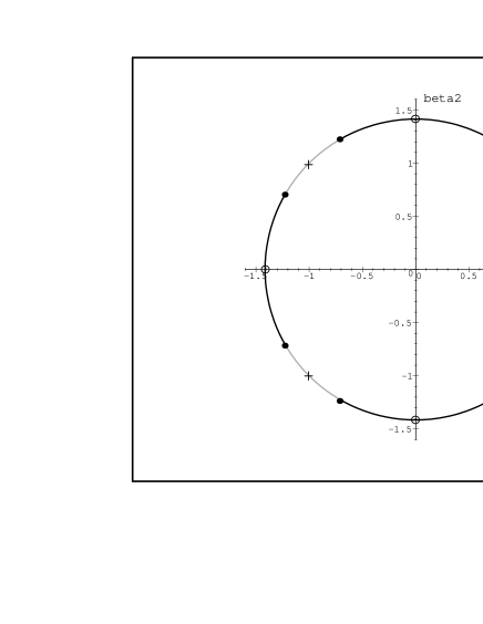
Figure 1: The marginal circle.

In Case 1 and Case 2 the last two terms of (3.7) are regular. In Case 1 the couplings $\beta_{1}$ and $\beta_{2}$ are equal and the model (1.1) decouples into two sine-Gordon models. In Case 2 the double-cosine model is non-trivial but no new terms are brought in by renormalization. In Case 3 one of the last two terms of (3.7) is logarithmically divergent and contributes to the beta function which is of the type (3.3). This case is the most interesting one and we will discuss it in some more details. In Case 4 the last two terms give rise to power-law divergences which lead to a generation of a mass term under renormalization. In Case 5 one of the couplings vanishes while the other has a value of $\pm\sqrt{2}$. In this case (1.1) is reduced to a single SG model at its marginal point and a free boson field. (The marginal limit of the SG model is discussed in details in [14].)

3.1 The Model as a Current-Current Perturbation

In this subsection we will show that the double-cosine interaction can be written as a current-current perturbation at the marginal points where the quantity $|\beta_{1}^{2}-\beta_{2}^{2}|$ has integer values — these are cases 1, 3, and 5 of (3.8). In each of these cases the values of $\beta_{1}$ and $\beta_{2}$ are such that the double-cosine perturbation can be written in the form

$$\mathcal{O}(z,\bar{z})=\prod_{i=1}^{2}\cos[\beta_{i}\Phi_{i}(z,\bar{z})]=\sum_{\alpha_{j}\ :\ {\rm some}}E^{\alpha_{j}}(z)\overline{E}^{-\alpha_{j}}(\bar{z})\ ,$$ (3.9)

where $\left\{\alpha_{j}\right\}$ are some (but not all) of the roots and $E^{\alpha_{j}}(z)$ are the corresponding generators of some Lie algebra $\mathfrak{g}$ in the Cartan-Weyl basis. As we will show below, the generators corresponding to all roots as well as the Cartan generators of $\mathfrak{g}$ are generated under renormalization, thus leading to a current-current perturbation to the level 1 $\mathfrak{g}$ current algebra:

$$S=S_{\rm CFT}\\ +\frac{\lambda}{4\pi}\int d^{2}z\left\{\sum_{\alpha_{j}>0}\left[E^{\alpha_{j}}(z)\overline{E}^{-\alpha_{j}}(\bar{z})+E^{-\alpha_{j}}(z)\overline{E}^{\alpha_{j}}(\bar{z})\right]+\sum_{i=1}^{\rm rank(\mathfrak{g})}H^{i}(z)\overline{H}^{i}(\bar{z})\right\}.$$ (3.11)

Let us first consider Case 1 of eq. (3.8). The condition $|\beta_{1}^{2}-\beta_{2}^{2}|=0$ together with the constraint that $\beta_{i}$ lie on the marginal manifold, $\beta_{1}^{2}+\beta_{2}^{2}=2$, specifies 4 points in the parameter space:

$$\beta_{1}^{2}=\beta_{2}^{2}=1\ .$$ (3.12)

At these points the model decouples into two SG models, each at its marginal point. As shown for instance in [14], the SG model in the marginal limit is equivalent under renormalization to a current-current perturbation of the $\mathfrak{su}{\scriptstyle(2)}$ current algebra and also to the $\mathfrak{su}{\scriptstyle(2)}$ Gross-Neveu model.

Next, let us consider Case 3 of eq. (3.8). The constraints $|\beta_{1}^{2}-\beta_{2}^{2}|=1$ and $\beta_{1}^{2}+\beta_{2}^{2}=2$ specify 8 points in the parameter space:

$$\beta_{1}^{2}=\frac{3}{2}\ ,~{}~{}\beta_{2}^{2}=\frac{1}{2}\ ;~{}~{}~{}~{}~{}~{}~{}\beta_{1}^{2}=\frac{1}{2}\ ,~{}~{}\beta_{2}^{2}=\frac{3}{2}\ .$$ (3.13)

The RHS of the generic OPE (3.7) then reads:

$$\frac{1}{4}\frac{1}{{|w-z|}^{2}}\left\{\sum_{i=1}^{2}\beta_{i}^{2}\partial_{z}\Phi_{i}(z,\bar{z})\partial_{\bar{z}}\Phi_{i}(z,\bar{z})+2\cos[2\beta_{\scriptscriptstyle<}\Phi_{\scriptscriptstyle<}(z,\bar{z})]\right\}\ .$$ (3.14)

The full renormalized action at the marginal points (3.13) is

$$S=\frac{1}{4\pi}\int d\tau dx\left\{\frac{1}{2}\sum_{i=1}^{2}{\left(\partial_{\mu}\Phi_{i}\right)}^{2}\right.\\ +\left.\lambda\left[\sum_{i=1}^{2}\beta_{i}^{2}\partial_{z}\Phi_{i}\partial_{\bar{z}}\Phi_{i}+\cos({\beta}_{1}\Phi_{1})\cos({\beta}_{2}\Phi_{2})+\cos(2\beta_{\scriptscriptstyle<}\Phi_{\scriptscriptstyle<})\right]\right\}\ ,$$ (3.15)

where the values of $\beta_{1}$ and $\beta_{2}$ are solutions of (3.13), $\beta_{\scriptscriptstyle<}\equiv\min(\beta_{1},\beta_{2})$, and $\Phi_{\scriptscriptstyle<}$ is the field corresponding to $\beta_{\scriptscriptstyle<}$. Consulting the vertex representations of the Kac-Moody currents of $\mathfrak{su}{\scriptstyle(3)}$ and their OPEs, we can rewrite the $\lambda$-term of (3.15) as a current-current perturbation of the current algebra $\mathfrak{su}{\scriptstyle(3)}$ (the $\mathfrak{su}{\scriptstyle(3)}$ WZW model).

$$\frac{\lambda}{4\pi}\int d^{2}z\left\{\sum_{\alpha_{i}>0}\left[E^{\alpha_{i}}(z)\overline{E}^{-\alpha_{i}}(\bar{z})+E^{-\alpha_{i}}(z)\overline{E}^{\alpha_{i}}(\bar{z})\right]+\sum_{i=1}^{2}H^{i}(z)\overline{H}^{i}(\bar{z})\right\}\ .$$ (3.16)

This is also equivalent[14] to the $\mathfrak{su}{\scriptstyle(3)}$ Gross-Neveu model. Therefore, at the points (3.13) the double-cosine model is integrable and yet nontrivial since it is not reduced to the SG model.

Finally, in Case 5 of eq. (3.8), the constraints $|\beta_{1}^{2}-\beta_{2}^{2}|=2$ and $\beta_{1}^{2}+\beta_{2}^{2}=2$ specify the 4 points

$$\beta_{1}^{2}=2\ ,~{}~{}\beta_{2}^{2}=0\ ;~{}~{}~{}~{}~{}~{}~{}\beta_{1}^{2}=0\ ,~{}~{}\beta_{2}^{2}=2$$ (3.17)

where the model decouples into a free field and a single marginal SG model (equivalent under renormalization to a $\mathfrak{su}{\scriptstyle(2)}$ Gross-Neveu model [14]).

3.2 The Model away from the Gross-Neveu Points

So far we have discussed the behavior of the marginal double-cosine model only at the special points where the model can be written as a current-current perturbation. Let us now complete the renormalization group analysis on the entire marginal manifold. The regions that remain to be considered are described by Cases 2 and 4 of eq. (3.8). (See Figure 1.)

Case 2 corresponds to the regions on the marginal circle, $\beta_{1}^{2}+\beta_{2}^{2}=2$, where the couplings also satisfy the constraint $0<|\beta_{1}^{2}-\beta_{2}^{2}|<1$ (the grey segments on Figure 1). On these segments the only contribution to the beta function of $\lambda$ comes from the first term of (3.7) while the last two terms do not give rise to singularities. The full renormalized action in this regime reads:

$$S=\frac{1}{4\pi}\int d\tau dx\left\{\frac{1}{2}\sum_{i=1}^{2}{\left(\partial_{\mu}\Phi_{i}\right)}^{2}+\lambda\left[\prod_{i=1}^{2}\cos({\beta}_{i}\Phi_{i})+\sum_{i=1}^{2}\beta_{i}^{2}\partial_{z}\Phi_{i}\partial_{\bar{z}}\Phi_{i}\right]\right\}\ .$$ (3.18)

The beta function for the coupling $\lambda$ is:

$$\beta_{\lambda}\equiv\mu\frac{d\lambda}{d\mu}=\frac{1}{2}\sqrt{\frac{\beta_{1}^{4}+\beta_{2}^{4}}{2}}\lambda^{2}+o^{3}(\lambda)\ .$$ (3.19)

Although the model in this regime is non-trivial and its properties could be further investigated, the following simple argument makes integrability look very unlikely: In the limit $|\beta_{1}^{2}-\beta_{2}^{2}|\longrightarrow 0$ the model is equivalent to $\mathfrak{su}{\scriptstyle(2)}\oplus\mathfrak{su}{\scriptstyle(2)}$ current-current perturbation (two decoupled SG models) and its particle spectrum consists of 4 particles 1 soliton and 1 anti-soliton for each SG model (the fundamental representation of each $\mathfrak{su}{\scriptstyle(2)}$ is $\mathbf{2}$). In the other limit, $|\beta_{1}^{2}-\beta_{2}^{2}|\longrightarrow 1$, the model is equivalent to a $\mathfrak{su}{\scriptstyle(3)}$ current-current perturbation and its spectrum consists of 6 particles — belonging to the two fundamental representations, $\mathbf{3}$ and $\mathbf{\bar{3}}$, of $\mathfrak{su}{\scriptstyle(3)}$. Therefore it is not conceivable, just by counting the degrees of freedom, that the particle spectrum could be smoothly deformed from the first point to the second.

Case 4 corresponds to the segments on the marginal circle, where the couplings also satisfy $1<|\beta_{1}^{2}-\beta_{2}^{2}|<2$ (the black segments on Figure 1). On these segments, in addition to the contribution to $\beta_{\lambda}$ coming from the logarithmic singularity due to the first term of (3.7), it is necessary to add new counterterms to the action to cancel the singularity coming from one of the last two terms of (3.7). This is a power-law singularity and hence, by dimensional analysis, the coupling of this new counterterm has to be massive. The full renormalized action reads:

$$S=\frac{1}{4\pi}\int d\tau dx\left\{\frac{1}{2}\sum_{i=1}^{2}{\left(\partial_{\mu}\Phi_{i}\right)}^{2}\right.\\ \left.+\lambda\left[\prod_{i=1}^{2}\cos({\beta}_{i}\Phi_{i})+\sum_{i=1}^{2}\beta_{i}^{2}\partial_{z}\Phi_{i}\partial_{\bar{z}}\Phi_{i}\right]+\Lambda\cos(2\beta_{\scriptscriptstyle<}\Phi_{\scriptscriptstyle<})\right\}\ ,$$ (3.20)

where $\beta_{\scriptscriptstyle<}\equiv\min(\beta_{1},\beta_{2})$ and $\Phi_{\scriptscriptstyle<}$ is the corresponding field. The renormalization group equations in this case are

$$\beta_{\lambda}\equiv\mu\frac{d\lambda}{d\mu} =\frac{1}{2}\sqrt{\frac{\beta_{1}^{4}+\beta_{2}^{4}}{2}}\lambda^{2}+o^{3}(\lambda)$$ (3.21)

$$\beta_{\Lambda}\equiv\mu\frac{d\Lambda}{d\mu} =2\beta_{\scriptscriptstyle<}^{2}\Lambda+\frac{\lambda^{2}}{8}\mu^{2\left(\left|\beta_{1}^{2}-\beta_{2}^{2}\right|-1\right)}+\frac{2\beta_{\scriptscriptstyle<}^{4}}{\sqrt{2\left(\beta_{1}^{4}+\beta_{2}^{4}\right)}}\lambda\Lambda+o^{3}(\lambda,\Lambda)\ .$$

It can be easily checked that the massive $\Lambda$-perturbation in (3.20), generated under renormalization, breaks the conservation of the spin 3 current (2.3) even to first order in CPT. Therefore, in this region the model is not integrable.

4 Generalization to Arbitrary $N$

In the previous section we completed our analysis of the integrability of the double-cosine model ($N$=2) on the marginal manifold by considering all distinct cases specified by (3.8). Let us now try to generalize our analysis to the $N$-field case. We will be looking in particular for special points on the marginal $N$-sphere (2.4) where the $N$-cosine term can be written as a current-current perturbation to some current algebra $\mathfrak{g}$.

Expanding the cosines in terms of exponentials, we get:

$$\prod_{i=1}^{N}\cos(\beta_{i}\Phi_{i})=\sum_{\nu=0}^{2^{N}-1}e^{i\vec{\beta}_{\nu}\cdot\vec{\Phi}}\ ,$$ (4.1)

where $\vec{\Phi}\equiv\left(\Phi_{1},\ldots,\Phi_{N}\right)$ and $\vec{\beta}_{\nu}\equiv\left(s_{\nu}^{1}\beta_{1},\ldots,s_{\nu}^{N}\beta_{N}\right)$ with $s_{\nu}^{i}\in\{-1,+1\}$. All combinations of signs, $s_{\nu}^{i}$, are present in the RHS of (4.1), so that there are $2^{N}$ different vectors $\vec{\beta}_{\nu}$ in the $N$-field case. Our goal is to look for special values of $\beta_{i}$ for which the vectors $\beta_{\nu}$ become roots of some Lie algebra $\mathfrak{g}$.

There are a few constraints on $\mathfrak{g}$ that can be immediately seen:

1. $\mathfrak{g}$ must be simply-laced, since $(\vec{\beta}_{\nu}\cdot\vec{\beta}_{\nu})=2$, $\forall\nu$ and thus all the roots of $\mathfrak{g}$ must have equal length.

2. $\mathbf{rank}[\mathfrak{g}]$ must be $N$, since we will be looking for $N$-field vertex representations of the generators of $\mathfrak{g}$.

The simply-laced Lie algebras of rank $N$ are $\mathbf{A}_{N}$, $\mathbf{D}_{(N\geq 4)}$, and $\mathbf{E}_{(N=6,7,8)}$. Before trying to write (4.1) as a current-current perturbation to one of these algebras, let us first make the following simple considerations:

First, since ${|\vec{\beta}_{\nu}|}^{2}$=2, each of its components must satisfy:

$${(s_{\nu}^{i}\beta_{i})}^{2}=\beta_{i}^{2}\in(0,2)\ .$$ (4.2)

The ends of the above interval, 0 and 2, are excluded because in both cases some of the couplings $\beta_{i}$ will vanish and the $N$-field model will trivially reduce to a lower-$N$ case. Furthermore, if $\{\vec{\beta}_{\nu}\}$ are roots of a simply-laced Lie algebra with squared norm 2, it is easily seen from the Cartan matrix that

$$(\vec{\beta}_{\nu}\cdot\vec{\beta}_{\lambda}) =\pm 2\ , ~{}\mathrm{for}\ \nu=\pm\lambda\ ;$$ (4.3)

$$(\vec{\beta}_{\nu}\cdot\vec{\beta}_{\lambda}) \in\{-1,0,+1\}\ , ~{}\mathrm{for}\ \nu\neq\pm\lambda\ .$$

Let us assume, for instance, that $\vec{\beta}_{\nu}$ and $\vec{\beta}_{\lambda}$ ($\nu\neq\lambda$) differ only by their $p^{\mathrm{th}}$ components: $s_{\nu}^{p}=-s_{\lambda}^{p}$. According to (4.3) we have:

$$(\vec{\beta}_{\nu}\cdot\vec{\beta}_{\lambda})=\sum_{i=1}^{N}\beta_{i}^{2}-2\beta_{p}^{2}=n_{p}\in\{-1,0,+1\}\ .$$ (4.4)

Since for any $p\in\{1,\ldots,N\}$, there is a pair of vectors for which (4.4) is true, we conclude, using also (2.4), that

$$\beta_{i}^{2}\in\left\{\frac{1}{2},1,\frac{3}{2}\right\}\ ,~{}i=1,2,\ldots,N\ ,~{}~{}N\geq 2\ .$$ (4.5)

In other words, we can only hope to be able to write the $N$-cosine model as a current-current perturbation at the points on the marginal manifold whose coordinates satisfy (4.5). As $N$ increases, (2.4) additionally constrains the set (4.5), so we finally get:

$$\mathrm{For}~{}N=2: ~{}~{}~{}~{}~{}\beta_{i}^{2}\in\left\{\frac{1}{2},1,\frac{3}{2}\right\}\ , ~{}i=1,2\ ;$$ (4.6)

$$\mathrm{For}~{}N=3: ~{}~{}~{}~{}~{}\beta_{i}^{2}\in\left\{\frac{1}{2},1\right\}\ , ~{}i=1,2,3\ ;$$

$$\mathrm{For}~{}N=4: ~{}~{}~{}~{}~{}\beta_{i}^{2}\in\left\{\frac{1}{2}\right\}\ , ~{}i=1,2,3,4\ ;$$

$$\mathrm{For}~{}N>4: ~{}~{}~{}~{}~{}\beta_{i}^{2}\in\emptyset\ , ~{}i=1,2,\ldots,N\ .$$

Therefore, for $N>4$ the marginal $N$-cosine model cannot be written as a current-current perturbation.

Let us now consider in some more detail the remaining two cases, $N$=3 and $N$=4. We shall discuss below that in both cases there exist specific sets of values for the couplings $\beta_{i}$ specifying isolated points on the marginal manifold (2.4) where the model (1.1) is equivalent under renormalization to a a current-current perturbation of some current algebra $\mathfrak{g}$:

$$\frac{\lambda}{4\pi}\int d^{2}z\left\{\sum_{\alpha_{j}>0}\left[E^{\alpha_{j}}(z)\overline{E}^{-\alpha_{j}}(\bar{z})+E^{-\alpha_{j}}(z)\overline{E}^{\alpha_{j}}(\bar{z})\right]+\sum_{i=1}^{\rm rank(\mathfrak{g})}H^{i}(z)\overline{H}^{i}(\bar{z})\right\}\ .$$ (4.7)

This is a model of the Gross-Neveu type with $\mathfrak{g}$-symmetry and such QFTs are known to be integrable. The $S$-matrices for the $\mathfrak{g}$-invariant models of Gross-Neveu type are known explicitly for the classical Lie algebras [15, 16] and their structure is expected to be the same for all Lie algebras.

In the $N=3$ case the only possible candidate for $\mathfrak{g}$ is $\mathbf{A}_{3}=\mathfrak{su}{\scriptstyle(4)}$, since this is the only simply-laced Lie algebra of rank 3. There are 24 points on the marginal manifold (2.4) for which the values of the couplings $\beta_{i}$ are consistent with (4.6). These points are specified by the equations:

$$(\beta_{1}^{2},\beta_{2}^{2},\beta_{3}^{2})=\left(\frac{1}{2},1,\frac{1}{2}\right)\ ,~{}\left(1,\frac{1}{2},\frac{1}{2}\right)\ ,~{}\left(\frac{1}{2},\frac{1}{2},1\right)\ .$$ (4.8)

At the above points, the 3-cosine action is equivalent to a current-current perturbation of the type (4.7) with $\mathfrak{g}=\mathfrak{su}{\scriptstyle(4)}$. In this case $\alpha_{j}$ runs over the 3 simple roots and the 3 non-simple positive roots of $\mathfrak{su}{\scriptstyle(4)}$ and $-\alpha_{j}$ are the corresponding negative roots. The perturbation of (4.7) thus contains the generators for all 12 roots of $\mathfrak{su}{\scriptstyle(4)}$ and the 3 Cartan generators, which is consistent with rank$[\mathfrak{su}{\scriptstyle(4)}]$=3 and dim$[\mathfrak{su}{\scriptstyle(4)}]$=15.

For $N=4$ the only possible candidates for $\mathfrak{g}$ are $\mathbf{A}_{4}=\mathfrak{su}{\scriptstyle(5)}$ and $\mathbf{D}_{4}=\mathfrak{so}{\scriptstyle(8)}$, the only simply-laced Lie algebras of rank 4. There are 16 points on the marginal 4-sphere (2.4) for which the values of the couplings $\beta_{i}$ are consistent with (4.6). Their coordinates are fixed by the equation:

$$(\beta_{1}^{2},\beta_{2}^{2},\beta_{3}^{2},\beta_{4}^{2})=\left(\frac{1}{2},\frac{1}{2},\frac{1}{2},\frac{1}{2}\right)\ .$$ (4.9)

The vectors $\vec{\beta}_{\nu}$ for the above values of the couplings do not satisfy the Cartan matrix of $\mathfrak{su}{\scriptstyle(5)}$ so we are left with the second candidate, $\mathfrak{so}{\scriptstyle(8)}$. We indeed showed that at the above points the 4-cosine action is equivalent under renormalization to a current-current perturbation of the $\mathfrak{g}=\mathfrak{so}{\scriptstyle(8)}$ current algebra. $\alpha_{j}$ runs over the 4 simple roots and the 8 non-simple positive roots of $\mathfrak{so}{\scriptstyle(8)}$ and $-\alpha_{j}$ are the corresponding negative roots. The perturbation of (4.7) thus contains the generators for all 24 roots of $\mathfrak{so}{\scriptstyle(8)}$ and the 4 Cartan generators, which is consistent with rank$[\mathfrak{so}{\scriptstyle(8)}]$=4 and dim$[\mathfrak{so}{\scriptstyle(8)}]$=28.

5 Conclusions

We have completed the analysis of the integrability of the double-cosine model on the marginal manifold and have found that the model is integrable only at the points where the interaction can be written as a current-current perturbation to some current algebra $\mathfrak{g}$. In addition to the previously known points with symmetry $\mathfrak{su}{\scriptstyle(2)}$ (single SG) and $\mathfrak{su}{\scriptstyle(2)}\oplus\mathfrak{su}{\scriptstyle(2)}$ (2 decoupled SGs), we have also found $\mathfrak{su}{\scriptstyle(3)}$-symmetric points where the model is of Gross-Neveu type and is thus integrable. Similarly, in the $N$=3 case we observed $\mathfrak{su}{\scriptstyle(4)}$-invariant integrable points and in the $N$=4 case, $\mathfrak{so}{\scriptstyle(8)}$-invariant integrable points.

At last, we would like to compare the marginal limiting behaviors of the multi-cosine models and the imaginary coupling affine Toda theories [14]. Toda theories depend on a single dimensionless coupling parameter. When this parameter approaches the value for which the perturbing operator becomes marginal, the theory is equivalent to a current-current perturbation of the WZW model based on some Lie algebra $\mathfrak{g}$. The full current algebra in the Toda case is generated under renormalization by the vertex operators in the original action corresponding to the simple roots and the affine root of $\mathfrak{g}$. The multi-cosine models, on the other hand, depend on many coupling parameters and become marginal on an entire hypersphere in the parameter space. At special points on this hypersphere they are also equivalent to a current-current perturbation of the $\mathfrak{g}$-symmetric WZW model, the full current algebra being generated by vertex operators in the original action corresponding to the simple and the negative-simple roots of $\mathfrak{g}$. Therefore, even though in general the $N$-cosine models are very different from the affine Toda theories, at special marginal points they have the same limiting behavior.

Appendices: $N$-Cosine Models as Current-Current Perturbations

A     $\mathfrak{su}{\scriptstyle(3)}$ Current-Current Perturbation for $N$=2

In this Appendix we provide some details of our calculation, showing that the 2-cosine model can be written as a $\mathfrak{su}{\scriptstyle(3)}$ current-current perturbation at the 8 points on the marginal 2-sphere (2.4) given by (3.13).

The Cartan matrix and the Dynkin diagram of $\mathfrak{su}{\scriptstyle(3)}$ are:

$$\mathbf{A}=\left(\begin{array}[]{rr}2&-1\\ -1&2\end{array}\right)\ ,\hskip 85.35826pt\begin{picture}(0.0,0.0)(0.0,0.0) \put(0.0,0.0){\circle{2.0}} \put(1.0,0.0){\line(1,0){8.0}} \put(10.0,0.0){\circle{2.0}} \put(-3.0,-5.0){${\scriptstyle(1,1)}$} \put(7.0,-5.0){${\scriptstyle(2,1)}$} \end{picture}$$ (A.1)

Let us take for example the point $\beta_{1}$=$\frac{1}{\sqrt{2}}$, $\beta_{2}$=$\sqrt{\frac{3}{2}}$. The double-cosine perturbation is expanded in terms of vertex operators as in (4.1), where the vectors $\vec{\beta}_{\nu}$ reproduce the simple roots of $\mathfrak{su}{\scriptstyle(3)}$ and their opposite negative roots:

$$\vec{\beta}_{0} =\vec{\beta}_{00}=\left(\frac{1}{\sqrt{2}},\sqrt{\frac{3}{2}}\right)=\alpha_{1}\ , \vec{\beta}_{3}=\vec{\beta}_{11}=-\alpha_{1}\ ;$$ (A.2)

$$\vec{\beta}_{1} =\vec{\beta}_{01}=\left(\frac{1}{\sqrt{2}},-\sqrt{\frac{3}{2}}\right)=\alpha_{2}\ , \vec{\beta}_{2}=\vec{\beta}_{10}=-\alpha_{2}\ .$$

We see that the exponential form (4.1) of the 2-cosine perturbation contains all $\mathfrak{su}{\scriptstyle(3)}$ generators corresponding to the simple roots $\alpha_{1}$, $\alpha_{2}$ and their opposite negative roots $-\alpha_{1}$, $-\alpha_{2}$. The generators corresponding to the remaining roots of $\mathfrak{su}{\scriptstyle(3)}$, $\alpha_{1}$+$\alpha_{2}$ and $-\alpha_{1}{\rm-}\alpha_{2}$, as well as the 2 Cartan generators of $\mathfrak{su}{\scriptstyle(3)}$, are generated under renormalization.

B     $\mathfrak{su}{\scriptstyle(4)}$ Current-Current Perturbation for $N$=3

In this Appendix we provide some details of our calculation, showing that the 3-cosine model can be written as a $\mathfrak{su}{\scriptstyle(4)}$ current-current perturbation at the 24 points on the marginal 3-sphere (2.4) given by (4.8).

The Cartan matrix and the Dynkin diagram of $\mathfrak{su}{\scriptstyle(4)}$ are:

$$\mathbf{A}=\left(\begin{array}[]{rrr}2&-1&0\\ -1&2&-1\\ 0&-1&2\end{array}\right)\ ,\hskip 85.35826pt\begin{picture}(0.0,0.0)(0.0,0.0) \put(0.0,0.0){\circle{2.0}} \put(1.0,0.0){\line(1,0){8.0}} \put(10.0,0.0){\circle{2.0}} \put(11.0,0.0){\line(1,0){8.0}} \put(20.0,0.0){\circle{2.0}} \put(-3.0,-5.0){${\scriptstyle(1,1)}$} \put(7.0,-5.0){${\scriptstyle(2,1)}$} \put(17.0,-5.0){${\scriptstyle(3,1)}$} \end{picture}$$ (B.1)

Let us take for example the point $\beta_{1}$=1, $\beta_{2}$=$\frac{1}{\sqrt{2}}$, $\beta_{3}$=1. The vectors $\vec{\beta}_{\nu}$ defined in (4.1) then reproduce all the simple and some of the other roots of $\mathfrak{su}{\scriptstyle(4)}$:

$$\vec{\beta}_{0} =\vec{\beta}_{000}=\left(\frac{1}{\sqrt{2}},1,\frac{1}{\sqrt{2}}\right)=\alpha_{1}\ , \vec{\beta}_{7}=\vec{\beta}_{111}=-\alpha_{1}\ ;$$ (B.2)

$$\vec{\beta}_{1} =\vec{\beta}_{001}=\left(\frac{1}{\sqrt{2}},1,\frac{-1}{\sqrt{2}}\right)=\alpha_{1}{\rm+}\alpha_{2}{\rm+}\alpha_{3}\ , \vec{\beta}_{6}=\vec{\beta}_{110}={\rm-}\alpha_{1}{\rm-}\alpha_{2}{\rm-}\alpha_{3}\ ;$$

$$\vec{\beta}_{2} =\vec{\beta}_{010}=\left(\frac{1}{\sqrt{2}},-1,\frac{1}{\sqrt{2}}\right)=-\alpha_{3}\ , \vec{\beta}_{5}=\vec{\beta}_{101}=\alpha_{3}\ ;$$

$$\vec{\beta}_{3} =\vec{\beta}_{011}=\left(\frac{1}{\sqrt{2}},-1,\frac{-1}{\sqrt{2}}\right)=\alpha_{2}\ , \vec{\beta}_{4}=\vec{\beta}_{100}=-\alpha_{2}\ .$$

We see that the exponential form (4.1) of the 3-cosine perturbation contains all $\mathfrak{su}{\scriptstyle(4)}$ generators corresponding to the simple roots $\alpha_{1}$, $\alpha_{2}$, and $\alpha_{3}$ and their opposite negative roots as well as the generators corresponding to the root $\alpha_{1}$+$\alpha_{2}$+$\alpha_{3}$ and its opposite. The generators corresponding to the remaining roots of $\mathfrak{su}{\scriptstyle(4)}$, $\alpha_{1}$+$\alpha_{2}$, $\alpha_{2}$+$\alpha_{3}$, and their opposite negative roots, as well as the 3 Cartan generators, are generated under renormalization.

C     $\mathfrak{so}{\scriptstyle(8)}$ Current-Current Perturbation for $N$=4

Here we provide some details of our calculation, showing that the 4-cosine model can be written as a $\mathfrak{so}{\scriptstyle(8)}$ current-current perturbation at the 16 points on the marginal 4-sphere (2.4) specified by (4.9).

The Cartan matrix and the Dynkin diagram of $\mathfrak{so}{\scriptstyle(8)}$ are:

$$\mathbf{A}=\left(\begin{array}[]{rrrr}2&-1&0&0\\ -1&2&-1&-1\\ 0&-1&2&0\\ 0&-1&0&2\end{array}\right)\ ,\hskip 85.35826pt\begin{picture}(0.0,0.0)(0.0,0.0) \put(0.0,0.0){\circle{2.0}} \put(1.0,0.0){\line(1,0){8.0}} \put(10.0,0.0){\circle{2.0}} \put(11.0,0.0){\line(1,0){8.0}} \put(20.0,0.0){\circle{2.0}} \put(10.0,1.0){\line(0,1){8.0}} \put(10.0,10.0){\circle{2.0}} \put(-3.0,-5.0){${\scriptstyle(1,1)}$} \put(7.0,-5.0){${\scriptstyle(2,2)}$} \put(17.0,-5.0){${\scriptstyle(3,1)}$} \put(13.0,9.0){${\scriptstyle(4,1)}$} \end{picture}$$ (C.1)

At the point $\beta_{1}=\beta_{2}=\beta_{3}=\beta_{4}=\frac{1}{\sqrt{2}}$, for example, the vectors $\vec{\beta}_{\nu}$ reproduce all the simple and some of the other roots of $\mathfrak{so}{\scriptstyle(8)}$:

$$\vec{\beta}_{0} =\vec{\beta}_{0000}=\frac{1}{\sqrt{2}}(1,1,1,1) = \ \alpha_{2} =-\vec{\beta}_{1111}=-\vec{\beta}_{15}\ ;$$ (C.2)

$$\vec{\beta}_{1} =\vec{\beta}_{0001}=\frac{1}{\sqrt{2}}(1,1,1,-1) = \ \alpha_{1}{\rm+}2\alpha_{2}{\rm+}\alpha_{3}{\rm+}\alpha_{4} =-\vec{\beta}_{1110}=-\vec{\beta}_{14}\ ;$$

$$\vec{\beta}_{2} =\vec{\beta}_{0010}=\frac{1}{\sqrt{2}}(1,1,-1,1) = \ -\alpha_{4} =-\vec{\beta}_{1101}=-\vec{\beta}_{13}\ ;$$

$$\vec{\beta}_{3} =\vec{\beta}_{0011}=\frac{1}{\sqrt{2}}(1,1,-1,-1) = \ \alpha_{1}{\rm+}\alpha_{2}{\rm+}\alpha_{3} =-\vec{\beta}_{1100}=-\vec{\beta}_{12}\ ;$$

$$\vec{\beta}_{4} =\vec{\beta}_{0100}=\frac{1}{\sqrt{2}}(1,-1,1,1) = \ -\alpha_{3} =-\vec{\beta}_{1011}=-\vec{\beta}_{11}\ ;$$

$$\vec{\beta}_{5} =\vec{\beta}_{0101}=\frac{1}{\sqrt{2}}(1,-1,1,-1) = \ \alpha_{1}{\rm+}\alpha_{2}{\rm+}\alpha_{4} =-\vec{\beta}_{1010}=-\vec{\beta}_{10}\ ;$$

$$\vec{\beta}_{6} =\vec{\beta}_{0110}=\frac{1}{\sqrt{2}}(1,-1,-1,1) = \ {\rm-}\alpha_{2}{\rm-}\alpha_{3}{\rm-}\alpha_{4} =-\vec{\beta}_{1001}=-\vec{\beta}_{9}\ ;$$

$$\vec{\beta}_{7} =\vec{\beta}_{0111}=\frac{1}{\sqrt{2}}(1,-1,-1,-1) = \ \alpha_{1} =-\vec{\beta}_{1000}=-\vec{\beta}_{8}\ .$$

Therefore, the 4-cosine perturbation contains all $\mathfrak{so}{\scriptstyle(8)}$ generators corresponding to the simple roots $\alpha_{1}$, $\alpha_{2}$, $\alpha_{3}$, $\alpha_{4}$, and their opposite negative roots, as well as the generators corresponding to the roots $\alpha_{1}$+$\alpha_{2}$+$\alpha_{3}$, $\alpha_{1}$+$\alpha_{2}$+$\alpha_{4}$, $\alpha_{2}$+$\alpha_{3}$+$\alpha_{4}$, $\alpha_{1}$+$2\alpha_{2}$+$\alpha_{3}$+$\alpha_{4}$, and their opposite. The remaining generators of $\mathfrak{so}{\scriptstyle(8)}$, corresponding to the roots $\alpha_{1}$+$\alpha_{2}$, $\alpha_{2}$+$\alpha_{3}$, $\alpha_{2}$+$\alpha_{4}$, $\alpha_{1}$+$\alpha_{2}$+$\alpha_{3}$+$\alpha_{4}$, and their opposite, as well as the 4 Cartan generators, are generated under renormalization.

References

• [1] R. Shankar, Phys. Lett. B102 (1981) 257 .
• [2] A. P. Bukhvostov, L. N. Lipatov, Nucl. Phys. B180 (1981) 116.
• [3] V. A. Fateev, Phys. Lett. B357 (1995) 397.
• [4] V. A. Fateev, Nucl. Phys. B473 (1996) 509.
• [5] P. Baseilhac, P. Grangé, M. Rausch de Traubenberg, “The Embedding of Liouville, sine-Gordon and deformed-Toda Models from Generalized Clifford Algebras”, hep-th/9802169.
• [6] H. Saleur, P. Simonetti, Nucl. Phys. B535 (1998) 596.
• [7] M. Ameduri, C. J. Efthimiou, J. Nonl. Math. Phys. 5 (1998) 132.
• [8] F. Lesage, H. Saleur, P. Simonetti, Phys. Rev. B56 (1997) 7598.
• [9] F. Lesage, H. Saleur, P. Simonetti, Phys. Rev. B57 (1998) 4694.
• [10] M. Ameduri, C. J. Efthimiou, B. Gerganov, “On the Integrability of the Bukhvostov–Lipatov Model”, hep-th/9810184.
• [11] H. Saleur, “The Long Delayed Solution of the Bukhvostov–Lipatov Model”, hep-th/9811023.
• [12] A. B. Zamolodchikov, Adv. Studies in Pure Math. 19 (1989) 641.
• [13] A. B. Zamolodchikov, Sov. J. Nucl. Phys. 46 (1987) 1090.
• [14] D. Bernard, A. LeClair, Commun. Math. Phys. 142 (1991) 99.
• [15] M. Karowski, H. J. Thun, Nucl. Phys. B190 (1981) 61.
• [16] E. Ogievetsky, N. Yu. Reshetikhin, P. Wiegmann, Nucl. Phys. B280 [FS18] (1987) 45.
• [17] P. Di Francesco, P. Mathieu, D. Sénéchal, “Conformal Field Theory”, Springer, New York 1996.
• [18] J. Fuchs, “Affine Lie Algebras and Quantum Groups”, Cambridge University Press, Cambridge 1992.