STRING DYNAMICS NEAR A KALUZA-KLEIN
BLACK HOLE

Abstract

The dynamics of a string near a Kaluza-Klein black hole are studied. Solutions to the classical string equations of motion are obtained using the world sheet velocity of light as an expansion parameter. The electrically and magnetically charged cases are considered separately. Solutions for string coordinates are obtained in terms of the world-sheet coordinate $\tau$. It is shown that the Kaluza-Klein radius increases/decreases with $\tau$ for electrically/magnetically charged black hole.

PACS number(s) : 04.50.+h, 11.25.Db, 04.70.Bw

Keywords : Kaluza-Klein theory, black hole, string dynamics, compactification

String propagation near a black hole is of great interest because of the interplay between the extended probe and the nontrivial background geometry. An extensive literature (for a review see [1]) deals with the study of classical string dynamics in curved backgrounds. This investigation is important with a view to eventually understand and interpret string quantization in curved spacetimes.

A consistent quantization of strings requires string theory to be a higher dimensional theory. The extra dimensions are compactified to obtain four-dimensional spacetime. It is an important question in string theory to study the mechanism of this compactification. The extra dimensions are expected to contribute nontrivially to the dynamics in the vicinity of a black hole, i.e., in the strong gravity regime. An interesting approach could be to study how the compact extra dimensions unfold as a string falls into a black hole. It is not unreasonable to hope that a string can be used as a probe to understand how four-dimensional spacetime arises dynamically from an underlying higher dimensional theory.

The problem is complicated as it involves solving equations of motion in $D$-dimensional ($D=26$ for bosonic strings and $D=10$ for superstrings) spacetime, which includes the compact manifold. As an in-between approach, we study string propagation in five- dimensional Kaluza-Klein black hole backgrounds as a minimal extension to four-dimensional curved spacetime. These backgrounds are solutions to the five-dimensional Einstein equations, and include regular four-dimensional black hole solutions.

The string world-sheet action [3] is given by

$$S=-T_{0}\int d\tau d\sigma\sqrt{-detg_{ab}}$$ (1)

where $g_{ab}=G_{\mu\nu}(X)\mbox{$\partial$}_{a}X^{\mu}\mbox{$\partial$}_{b}X^{\nu}$ is the two-dimensional world-sheet metric; $\sigma$ and $\tau$ are the world sheet coordinates.

The classical equations of motion in the gauge $g_{ab}=\rho(\sigma,\tau)\eta_{ab}$ ($\eta_{ab}$ is the two- dimensional Minkowskian metric) are given by

$$\mbox{$\partial$}_{\tau}^{2}X^{\mu}-c^{2}\mbox{$\partial$}_{\sigma}^{2}X^{\mu}+\Gamma_{\nu\rho}^{\mu}\left[\mbox{$\partial$}_{\tau}X^{\nu}\mbox{$\partial$}_{\tau}X^{\rho}-c^{2}\mbox{$\partial$}_{\sigma}X^{\nu}\mbox{$\partial$}_{\sigma}X^{\rho}\right]=0.$$ (2)

and the constraints are given by

$$\mbox{$\partial$}_{\tau}X^{\mu}\mbox{$\partial$}_{\sigma}X^{\nu}G_{\mu\nu}=0$$ (3)

$$[\mbox{$\partial$}_{\tau}X^{\mu}\mbox{$\partial$}_{\tau}X^{\nu}+c^{2}\mbox{$\partial$}_{\sigma}X^{\mu}\mbox{$\partial$}_{\sigma}X^{\nu}]G_{\mu\nu}=0.$$ (4)

Here $c$ is the velocity of wave propagation along the string.

Various simplifying ansatze exist for obtaining solutions to the highly nonlinear system of equations (2)-(4), one being perturbation expansion of string coordinates. We follow the approach of de Vega and Nicolaidis [4] which uses the world-sheet velocity of light as an expansion parameter. The scheme involves systematic expansion in powers of $c$. If $c<<1$, the coordinate expansion is suitable to describe strings in a strong gravitational background (see [5, 6]). Here, the derivatives w.r.t. $\tau$ overwhelm the $\sigma$ derivatives. In the opposite case ($c>>1$), the classical equations of motion give us a stationary picture as the $\sigma$ derivatives dominate.

We restrict ourselves to the case where $c$ is small, our interest being to probe the dynamical behaviour of the extra dimensions. The string coordinates are expressed as

$$X^{\mu}(\sigma,\tau)=A^{\mu}(\sigma,\tau)+c^{2}B^{\mu}(\sigma,\tau)+c^{4}C^{\mu}(\sigma,\tau)+...,$$ (5)

and the zeroth order $A^{\mu}(\sigma,\tau)$ satisfies the following set of equations(with dot and prime denoting differentiation w.r.t. $\tau$ and $\sigma$ respectively);

$$\ddot{A}^{\mu}+\Gamma_{\nu\rho}^{\mu}\dot{A}^{\nu}\dot{A}^{\rho} = 0,$$ (6)

$$\dot{A}^{\mu}\dot{A}^{\nu}G_{\mu\nu} = 0,$$

$$\dot{A}^{\mu}A^{\prime\nu}G_{\mu\nu} = 0.$$

These equations describe the motion of a null string [4]. The second constraint is the ’stringy’ constraint and restricts the motion to be perpendicular to the string.

The metric background to study string propagation [7] (see also [8]) is

$$ds^{2}=-e^{4k\frac{\varphi}{\sqrt{3}}}(dx_{5}+2kA_{\alpha}dx^{\alpha})^{2}+e^{-2k\frac{\varphi}{\sqrt{3}}}g_{\alpha\beta}dx^{\alpha}dx^{\beta},$$ (7)

where $k^{2}=4\pi G$; $x_{5}$ is the extra dimension and should be identified modulo $2\pi R_{0}$, where $R_{0}$ is the radius of the circle about which the coordinate $x_{5}$ winds. The quantity $R_{0}$ is the asymptotic value of a dynamical quantity, the Kaluza-Klein radius, which is discussed below. Here $g_{\alpha\beta}$ is the four-dimensional spacetime.

The mass $M$ of the black hole, the electric charge $Q$ and the magnetic charge $P$ are related to the scalar charge $\Sigma$ by

$$\frac{2}{3}\Sigma=\frac{Q^{2}}{\Sigma+\sqrt{3}M}+\frac{P^{2}}{\Sigma-\sqrt{3}M},$$ (8)

where the scalar charge is defined as

$k\varphi\longrightarrow\frac{\Sigma}{r}+O\left(\frac{1}{r^{2}}\right)$ as $r\longrightarrow\infty.$

We follow the notation of ref. [9]. The black hole solutions are

$$e^{4\varphi/\sqrt{3}} = \frac{B}{A},A_{\mu}dx^{\mu}=\frac{Q}{B}(r-\Sigma)dt+P\cos\theta d\phi$$ (9)

$$g_{\mu\nu}dx^{\mu}dx^{\nu} = \frac{f^{2}}{\sqrt{AB}}dt^{2}-\frac{\sqrt{AB}}{f^{2}}dr^{2}-\sqrt{AB}\left(d\theta^{2}+\sin^{2}\theta d\phi^{2}\right)$$

Here $A$, $B$ and $f$ are given by

$$A = (r-\frac{\Sigma}{\sqrt{3}})^{2}-\frac{2P^{2}\Sigma}{\Sigma-\sqrt{3}M}$$ (10)

$$B = (r+\frac{\Sigma}{\sqrt{3}})^{2}-\frac{2Q^{2}\Sigma}{\Sigma+\sqrt{3}M}$$

$$f^{2} = (r-M)^{2}-(M^{2}+\Sigma^{2}-P^{2}-Q^{2})$$

We seek to solve the equations of motion for the string coordinates in the exterior of the black hole. For simplicity, we consider the magnetically and electrically charged cases separately. The zeroth order equations of motion for string coordinates in the electrically neutral ($Q=0$) background are

$$\frac{\mbox{$\partial$}^{2}t}{\mbox{$\partial$}\tau^{2}}+2\left(\frac{f^{\prime}}{f}-\frac{B^{\prime}}{2B}\right)\frac{\mbox{$\partial$}t}{\mbox{$\partial$}\tau}\frac{\mbox{$\partial$}r}{\mbox{$\partial$}\tau} = 0,$$ (11)

$$\frac{\mbox{$\partial$}^{2}r}{\mbox{$\partial$}\tau^{2}}+\left[-\frac{f^{3}}{2AB^{2}}(B^{\prime}f-2f^{\prime}B)\right]\left(\frac{\mbox{$\partial$}t}{\mbox{$\partial$}\tau}\right)^{2}+\left(\frac{A^{\prime}f-2f^{\prime}A}{2Af}\right)\left(\frac{\mbox{$\partial$}r}{\mbox{$\partial$}\tau}\right)^{2} -$$

$$\frac{f^{2}A^{\prime}}{2A}\left(\frac{\mbox{$\partial$}\phi}{\mbox{$\partial$}\tau}\right)^{2}+\frac{f^{2}}{2A^{3}}(A^{\prime}B-B^{\prime}A)\left(\frac{\mbox{$\partial$}x_{5}}{\mbox{$\partial$}\tau}\right)^{2} = 0,$$

$$\frac{\mbox{$\partial$}^{2}\phi}{\mbox{$\partial$}\tau^{2}}+\frac{A^{\prime}}{A}\left(\frac{\mbox{$\partial$}r}{\mbox{$\partial$}\tau}\right)\left(\frac{\mbox{$\partial$}\phi}{\mbox{$\partial$}\tau}\right) = 0,$$

$$\frac{\mbox{$\partial$}^{2}x_{5}}{\mbox{$\partial$}\tau^{2}}+\left(-\frac{A^{\prime}}{A}+\frac{B^{\prime}}{B}\right)\left(\frac{\mbox{$\partial$}r}{\mbox{$\partial$}\tau}\right)\left(\frac{\mbox{$\partial$}x_{5}}{\mbox{$\partial$}\tau}\right) = 0.$$

Here we restrict ourselves to the exterior region $r>M$ and the equatorial plane, i.e. $\theta=\pi/2$.

The first integrals of motion are given by

$$\frac{\mbox{$\partial$}t}{\mbox{$\partial$}\tau} = \frac{c_{1}B}{f^{2}},$$ (12)

$$\frac{\mbox{$\partial$}\phi}{\mbox{$\partial$}\tau} = \frac{c_{2}}{A},$$

$$\frac{\mbox{$\partial$}x_{5}}{\mbox{$\partial$}\tau} = c_{3}\frac{A}{B}$$

$$\left(\frac{\mbox{$\partial$}r}{\mbox{$\partial$}\tau}\right)^{2} = \frac{B}{A}c_{1}^{2}-\frac{f^{2}}{A^{2}}c_{2}^{2}-\frac{f^{2}}{B}c_{3}^{2}.$$

where $c_{1}$, $c_{2}$ and $c_{3}$ are integration constants.

The equations can be further reduced to quadratures

$$\tau = \int\frac{dr}{\sqrt{\frac{B}{A}c_{1}^{2}-\frac{f^{2}}{B}c_{3}^{2}}},$$ (13)

$$x_{5} = \int\frac{c_{3}Adr}{B\sqrt{\frac{B}{A}c_{1}^{2}-\frac{f^{2}}{B}c_{3}^{2}}},$$

$$t = \int\frac{c_{1}Bdr}{f^{2}\sqrt{\frac{B}{A}c_{1}^{2}-\frac{f^{2}}{B}c_{3}^{2}}},$$

up to constants of integration which depend on $\sigma$ and can be solved numerically to obtain $t$, $r$, $\phi$ and $x_{5}$ as functions of $\tau$. Here, we have taken $c_{2}=0$, i.e. the string is falling in ’head-on’ and we work in the region where $r>>\Sigma$.

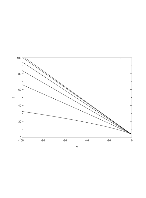
Figure 1: Plot of $r$ vs.$\tau$ for magnetically charged black hole, for different choices of $c_{1}$ and $c_{3}$..

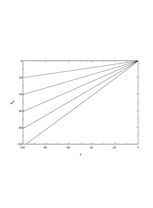
Figure 2: $x_{5}$ vs. $\tau$ for magnetically charged black hole.

The integrals (STRING DYNAMICS NEAR A KALUZA-KLEIN BLACK HOLE) have been evaluated numerically and inverted to obtain the coordinates as function of $\tau$. The behaviour of $r$ as a function of $\tau$ is shown in Fig. 1 and that of the coordinate $x_{5}$ is shown in Fig. 2 for different values of $c_{1}$ and $c_{3}$.

For the electrically charged ($P=0$) black hole, the equations of motion in the zeroth order take the form

$$AB[Af^{2}+12Q^{2}(r-\Sigma_{1})^{2}]\frac{\mbox{$\partial$}^{2}t}{\mbox{$\partial$}\tau^{2}}-[12A^{\prime}BQ^{2}(r-\Sigma_{1})^{2}+B^{\prime}A^{2}f^{2} -$$ (14)

$$4B^{\prime}AQ^{2}(r-\Sigma_{1})^{2}-2f^{\prime}A^{2}Bf-8ABQ^{2}(r-\Sigma_{1})]\frac{\mbox{$\partial$}t}{\mbox{$\partial$}\tau}\frac{\mbox{$\partial$}r}{\mbox{$\partial$}\tau} +$$

$$4QAB[B^{\prime}(r-\Sigma_{1})-B]\frac{\mbox{$\partial$}r}{\mbox{$\partial$}\tau}\frac{\mbox{$\partial$}x_{5}}{\mbox{$\partial$}\tau} = 0,$$

$$2A^{3}B^{2}f\frac{\mbox{$\partial$}^{2}r}{\mbox{$\partial$}\tau^{2}}+f^{3}[4A^{\prime}BQ^{2}(r-\Sigma_{1})^{2}-B^{\prime}A^{2}f^{2}+4B^{\prime}AQ^{2}(r-\Sigma_{1})^{2} +$$

$$2f^{\prime}A^{2}Bf-8ABQ^{2}(r-\Sigma_{1})]\left(\frac{\mbox{$\partial$}t}{\mbox{$\partial$}\tau}\right)^{2}-8f^{3}B^{2}Q[A^{\prime}(r-\Sigma_{1})-A]\frac{\mbox{$\partial$}t}{\mbox{$\partial$}\tau}\frac{\mbox{$\partial$}x_{5}}{\mbox{$\partial$}\tau} +$$

$$A^{2}B^{2}[A^{\prime}f-2f^{\prime}A]\left(\frac{\mbox{$\partial$}r}{\mbox{$\partial$}\tau}\right)^{2}-A^{2}B^{2}f^{3}A^{\prime}\left(\frac{\mbox{$\partial$}\phi}{\mbox{$\partial$}\tau}\right)^{2}+f^{3}B^{2}[A^{\prime}B-B^{\prime}A]\left(\frac{\mbox{$\partial$}x_{5}}{\mbox{$\partial$}\tau}\right)^{2} = 0,$$

$$AB^{2}[Af^{2}+12Q^{2}(r-\Sigma_{1})^{2}]\frac{\mbox{$\partial$}^{2}x_{5}}{\mbox{$\partial$}\tau^{2}}-4QA[A^{\prime}Bf^{2}(r-\Sigma_{1})-B^{\prime}Af^{2}(r-\Sigma_{1}) +$$

$$4B^{\prime}Q^{2}(r-\Sigma_{1})^{3}+2f^{\prime}ABf(r-\Sigma_{1})-ABf^{2}-4BQ^{2}(r-\Sigma_{1})^{2}]\frac{\mbox{$\partial$}t}{\mbox{$\partial$}\tau}\frac{\mbox{$\partial$}r}{\mbox{$\partial$}\tau} -$$

$$B[A^{\prime}ABf^{2}+12A^{\prime}BQ^{2}(r-\Sigma_{1})^{2}-B^{\prime}A^{2}f^{2}+4B^{\prime}AQ^{2}(r-\Sigma_{1})^{2} -$$

$$16ABQ^{2}(r-\Sigma_{1})]\frac{\mbox{$\partial$}r}{\mbox{$\partial$}\tau}\frac{\mbox{$\partial$}x_{5}}{\mbox{$\partial$}\tau} = 0.$$

where $\Sigma_{1}=\Sigma/\sqrt{3}$ and the constraint equation is

$$\left\{\frac{f^{2}}{B}-\frac{4Q^{2}}{AB}(r-\Sigma_{1})^{2}\right\}\left(\frac{\mbox{$\partial$}t}{\mbox{$\partial$}\tau}\right)^{2}-\frac{8Q}{A}(r-\Sigma_{1})\frac{\mbox{$\partial$}t}{\mbox{$\partial$}t}\frac{\mbox{$\partial$}x_{5}}{\mbox{$\partial$}\tau} -$$ (15)

$$-\frac{A}{f^{2}}\left(\frac{\mbox{$\partial$}r}{\mbox{$\partial$}\tau}\right)^{2}-A\left(\frac{\mbox{$\partial$}\phi}{\mbox{$\partial$}\tau}\right)^{2}-\frac{B}{A}\left(\frac{\mbox{$\partial$}x_{5}}{\mbox{$\partial$}\tau}\right)^{2} = 0.$$

The structure of the equations in this case is such that they are not reducible to quadratures and we have to resort to solving them numerically. Again, we consider an infalling string in the region where $r>>\Sigma$ and $\theta=\pi/2$.

The set of equations (STRING DYNAMICS NEAR A KALUZA-KLEIN BLACK HOLE) and (STRING DYNAMICS NEAR A KALUZA-KLEIN BLACK HOLE) has been solved numerically to obtain the coordinates as functions of $\tau$. Again we have a two parameter family of solutions. Fig. 3 and Fig. 4 illustrate how $r$ and $x_{5}$ vary as functions of $\tau$ for different choices of integration constants.

The coordinate $x_{5}$ increases monotonically in the magnetic case, while in the electric case, it first increases and then starts decreasing. The two cases indicate, in the magnetic case, that the coordinate $x_{5}$ goes about a circle continuously in one direction, while in the electric case the direction reverses. Although the behaviour is different in the two cases, the picture becomes clear if we define a quantity, the Kaluza-Klein radius, which is related to its asymptotic value $R_{0}$ as

$$R(r)=R_{0}\left(\frac{B}{A}\right)^{1/2}.$$ (16)

The radius $R(r)$ is a dynamical quantity as it depends implicitly on $\tau$ through $R(\tau)=R(r(\tau))$. The effect of the magnetic field is to shrink the extra dimension (as already mentioned in [7]) i.e., as the string approaches the black hole, the value of the Kaluza-Klein radius which it sees becomes smaller than its asymptotic value. The presence of electric charge tends to expand the extra dimension. Fig. 5 and Fig. 6 clearly show that the behaviour of the Kaluza-Klein radius is opposite in the electrically and magnetically charged cases.

We have studied propagation of a null string in five-dimensional, electrically and magnetically charged, Kaluza-Klein black hole backgrounds. Our study of string propagation in Kaluza-Klein backgrounds is motivated by the importance of such backgrounds in the context of toroidal compactification schemes for string theory. Here, we have tried to explore the behaviour of the extra fifth dimension as the string approaches the black hole horizon. The solutions we have obtained are valid in the region outside the horizon but not asymptotically far from the horizon.

The solutions, in the limit $\Sigma\longrightarrow 0$, match with the ones given in [6]. The essential difference lies in the presence of the extra dimension. Another paper that deals with five-dimensional Kaluza-Klein black holes [9] finds out string corrections to the five-dimensional vacuum Einstein equations and their effect on the black hole metrics. On the other hand our approach is to study the dynamics of a string probe in a classical background. The two approaches are complementary to each other.

In the present paper, we have only considered the classical picture. In principle, however, one expects quantum effects to be dominant in the strong gravity regime. Nevertheless, we expect the classical picture to give an intuitive idea of the mechanism of compactification. It is clear from the above considerations that, even in the classical regime, we can probe the expansion/shrinking of the compact dimension. However, the effects of the background (and hence the compact dimension) on the string probe itself, in terms of changes in its shape and conformation, are identically zero in the zeroth order of the expansion in $c$. These effects are expected to manifest themselves if we go to higher orders in $c$. Work on this is in progress and will be reported elsewhere.

H. K. J. thanks the University Grants Commission, India, for a fellowship.

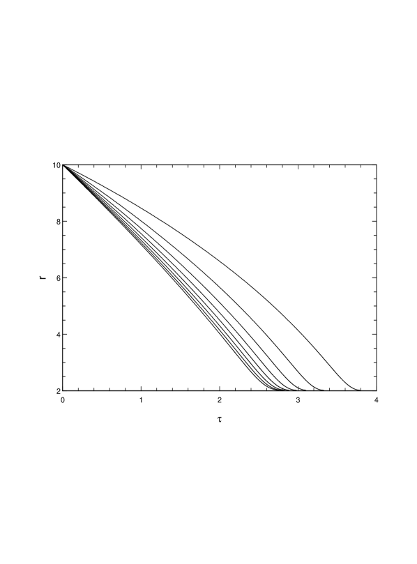
Figure 3: Plot of $r$ w.r.t. $\tau$ for electrically charged black hole, for different choices of integration constants.

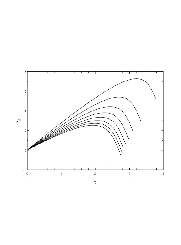
Figure 4: $x_{5}$ vs. $\tau$ for electrically charged black hole.

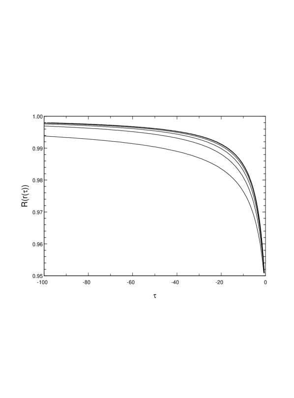
Figure 5: Kaluza-Klein radius as a function of $\tau$ for magnetic black hole.

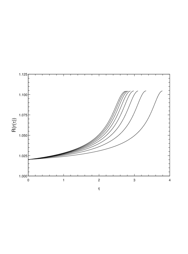
Figure 6: Kaluza-Klein radius for electrically charged case.

References

[1]H. J. De Vega and N. Sánchez, Lectures on String
Theory in Curved Spacetimes, in: Proc. Third Paris Cosmology
Colloquium (Paris, June 1995), ed. H. J. De Vega and N. Sánchez,
(World Scientific, 1996).
[2] I. Antoniadis, C. Bachas, J. Ellis and
D. V. Nanopoulos, Phys. Lett. B211 (1988) 393
[3] M. B. Green, J. H. Schwarz and E. Witten,
Superstring Theory
(Cambridge Univ. Press, 1987).
[4] H. J. De Vega and A. Nicolaidis,
Phys. Lett. B 295 (1992) 241.
[5] H. J. De Vega, I. Giannakis and A. Nicolaidis,
Mod. Phys. Lett. A, 10 (1995) 2479.
[6] C. O. Lousto and N. Sánchez,
Phys. Rev. D 54 (1996) 6399.
[7] G. W. Gibbons and D. L. Wiltshire,
Ann. Phys. 167 (1987) 201; 176 (1987) 393 (E).
[8] M. Cvetič and D. Youm, Phys. Rev. Lett. 75, (1995) 4165.
[9] N. Itzhaki, Nucl. Phys. B, 508 (1997) 700.