Gauge independent effective gauge fields

Abstract

The problem of gauge independent definition of the effective gauge field is considered. The Slavnov identities corresponding to a system of interacting quantum gauge and classical matter fields, playing the role of a measuring device, are obtained. With their help, in the case of power-counting renormalizable theories, gauge independence of the effective device action is proved in the low-energy limit, which allows to introduce the gauge independent notion of the effective gauge field.

Moscow State University, Physics Faculty,
Department of Theoretical Physics.
$117234$, Moscow, Russian Federation

PACS 03.70.+k, 11.15. q

1 Introduction

Description of quantized fields by means of the effective action (EA) is the most general in quantum theory. Being the sum of all one-particle-irreducible diagrams EA for a given theory allows to calculate any Green function in this theory. Well known that it also can be given a nonperturbative definition as the Legendre transform of the Green functions generating functional logarithm. Formal analogy between the classical equations of motion and quantum equations describing dynamics of the mean fields suggests natural interpretation of EA as the quantum substitute for its classical counterpart. However, explicit dependence of EA on the way the theory is quantized lacks direct physical application of this remarkable analogy. The most important kind of such a dependence, which attracts our attention in this Paper, is the gauge dependence of EA for gauge theories.

It is not our purpose to anew investigate various procedures formulated by many authors in attempts to construct a gauge independent object from EA. Instead, we would like to pay attention to a possible physical reason for the gauge dependence of EA, recently pointed out by Dalvit and Mazzitelli [1]. In the case of quantum gravity they showed that the motion of a classical device measuring the effective gravitational field is independent of the choice of gauge conditions fixing the general coordinate invariance. More precisely, the equations of motion (geodesic equation) of a test particle in the effective static gravitational field of a point mass, calculated in the one-loop approximation up to leading logarithms was shown to be independent of the choice of linear gauge.

The point is that while the graviton-test particle quantum interaction is negligible in calculation of the total effective gravitational field, it is not when the equations of the test particle motion are to be determined. It turns out that in the latter case the gauge dependent part of the contribution due to graviton-test particle interaction just cancels that corresponding to the ordinary gauge dependence of the mean field.

This fact offers a tempting possibility to change our plain view on the problem of gauge independent definition of the effective gravitational field, and look at it through a prism of the measurement. In other words, we can try to describe the effective gravitational field in terms corresponding to the measuring device. For example, in the case considered in [1] it is the form of the equations of the test particle motion by which the effective gravitational field is implicitly described.

Whether a proper definition of the effective field can be given in this way, depends on resolution of the following questions:

1. Whether the special choices of the source for the gravitational field and of the measuring device made in [1] are essential for the aforementioned cancellation.

2. Whether this cancellation holds at any order of the loop expansion and for all energies (not only for the one-loop low-energy leading quantum corrections).

3. If the effective gravitational field is described through characteristics of the measuring device, is such a description actually independent of the choice of device, for the concept of the effective action to be self-contained.

4. Is all of this inherent to the gravitation, or represents a general property of gauge interactions.

The purpose of this Paper is to show that the answer to 1.,4., and to the first part of 2. is really positive, i.e. the low-energy leading quantum corrections to the equations of motion of any kind of classical matter (infinitely weak) interacting with the gravitational or any other gauge field are gauge independent at any order of the loop expansion. In sec.2 we introduce notations and display some basic tools used later in investigation of EA properties. In sec.3 the Slavnov identities for the generating functionals of the Green functions corresponding to the system gauge field plus device are derived, on which basis the renormalization equations for divergent parts of these functionals are obtained in sec.4. These equations allow to demonstrate the gauge dependence cancellation most generally. In sec.5 we briefly discuss the rest of the problems listed above, and make conclusions.

2 The quantum effective action

The reason for the cancellation of the gauge dependence found by Dalvit and Mazzitelli may lie, of course, only in the residual symmetry of the Faddev-Popov quantum action for the gauge field, the Becci-Rouet-Stora-Tyutin (BRST) symmetry [2]. Having the form of the ordinary gauge transformation for the gauge and matter fields, the latter is indifferent to the specific structure of the classical action for these fields. Therefore, following the standard procedure of derivation of the Slavnov identities for the generating functionals of the Green functions, we can try to obtain analogous identities for the system of the gauge field plus measuring device in the most general form.

We consider a general type gauge theory described by an action $S(A_{a},\phi_{i})$, where $A_{a},a=1,...,n$ denotes the gauge field and $\phi_{i},i=1,...,m$ – matter fields of any kind.

If the pure gauge theory describes free fields $A_{a},$ then a number of quantum matter fields interacting with $A_{a}$ should be included in $\phi$. However, for notation simplicity we suppose that the gauge field is self-interacting and $\phi$ contains only classical matter fields. Furthermore, the part of $\phi$ corresponding to the sources for $A_{a}$ can be omitted since any desired A-field configuration can be formally obtained by appropriate choice of the standard source term $J_{a}A_{a}$ which is normally introduced into the generating functional of the Green functions. Thus, we suppose the fields $\phi_{i}$ to describe the measuring device only. The latter is a classical object in the ordinary sense that the low-energy quantum corrections to its equations of motion due to propagation of the $\phi$-fields can be neglected, which usually means that the device should be sufficiently heavy. Following [1] we also require the device contribution to the total gauge field to be infinitely small. One could suppose, for example, that the coupling constants of the gauge field-device interaction are sufficiently small. Since, however, it is not always possible to choose these constants arbitrary small, we simply imagine that the device action enters the full action with a small overall coefficient.

It is problematical to satisfy the above requirements in the case of gravity, since they contradict to each other. Even more: in this case we cannot satisfy the first of them alone because there is no such a thing as the classical source for gravity, as was pointed out in [3]. Therefore, in the case of measurement of the effective gravitational field we are forced to introduce the classical form for the device action ”by hands”.

Let the action $S(A,\phi)$ be invariant under the following (infinitesimal) gauge transformations

$$\delta A_{a}=D_{a\alpha}(A)\xi_{\alpha},~{}~{}\delta\phi_{i}=\tilde{D}_{i\alpha}(\phi)\xi_{\alpha},$$ (1)

where $D_{a\alpha}(A),\tilde{D}_{i\alpha}(\phi)$ are the generators, and $\xi_{\alpha},\alpha=1,...,N$ are arbitrary gauge functions of the gauge transformations. We suppose that these generators form a closed algebra

$$D_{a\alpha,b}D_{b\beta}-D_{a\beta,b}D_{b\alpha}=f_{\alpha\beta\gamma}D_{a\gamma},$$

$$\tilde{D}_{i\alpha,j}\tilde{D}_{j\beta}-\tilde{D}_{i\beta,j}\tilde{D}_{j\alpha}=f_{\alpha\beta\gamma}\tilde{D}_{i\gamma},$$ (2)

where the ”structure constants” $f_{\gamma\alpha\beta}$ are some linear differential operators which we assume to be field-independent, for simplicity. Commas followed by indices denote functional differentiation with respect to the corresponding fields, and DeWitt’s summation-integration on repeated indices is supposed.

To fix this invariance we impose an arbitrary gauge condition $F_{\alpha}(A)=0$. For simplicity, we suppose that it is linear in the field $A$: $F_{\alpha}(A)\equiv F_{\alpha,a}A_{a}$, where $F_{\alpha,a}$ is some (differential) operator independent of the fields. Weighted in the usual way this gauge condition enters the Faddeev-Popov (FP) quantum action $S_{fp}$ in the form of the gauge-fixing term

$$S_{gf}=-\frac{1}{2\xi}F_{\alpha}^{2},$$ (3)

$\xi$ being the weighting parameter. Introducing FP ghost fields $C_{\alpha},\bar{C}_{\alpha}$ we write the FP quantum action

$$S_{fp}=S(A,\phi)+S_{gf}+\bar{C}_{\beta}F_{\beta,a}D_{a\alpha}C_{\alpha}.$$ (4)

$S_{fp}$ is still invariant under the following BRST transformations [2]

$$\delta_{brst}A_{a}=D_{a\alpha}(A)C_{\alpha}\lambda,$$

$$\delta_{brst}\phi_{i}=\tilde{D}_{i\alpha}(\phi)C_{\alpha}\lambda,$$

$$\delta_{brst}C_{\alpha}=-f_{\alpha\beta\gamma}C_{\beta}C_{\gamma}\lambda,$$

$$\delta_{brst}\bar{C}_{\alpha}=-\frac{1}{\xi}F_{\alpha}\lambda,$$ (5)

$\lambda$ being a constant anticommuting parameter.

To be able to write down the Slavnov identities for the generating functional of connected Green functions we introduce sources for the BRST transformations following Zinn-Justin [6], and obtain the quantum action $\Sigma$ in the form

$$\Sigma=S(A,\phi)-\frac{1}{2\xi}F_{\alpha}^{2}+\bar{C}_{\alpha}F_{\alpha,a}D_{a\beta}C_{\beta}+K_{a}D_{a\alpha}C_{\alpha}+\tilde{K}_{i}\tilde{D}_{i\alpha}C_{\alpha}.$$ (6)

Introduction of the source $\tilde{K}$ is dispensable since $\tilde{D}_{i\alpha}C_{\alpha}$ is linear in quantum fields. However, it allows to write the Slavnov identities in the form containing no explicit information on the structure of the gauge algebra, and in addition to that, to omit all ghost sources from the very beginning (these sources should be restored, however, in renormalization of the theory).

Below we consider the most important kind of the gauge dependence of EA, namely its dependence on the weighting parameter $\xi$. The general case contains no principal complications, and can be handled, for example, by extending the field content of the theory to include a number of auxiliary fields introducing the gauge, and employing the method of anticanonical transformations ( see, e.g., [4]). A natural way of investigation of the $\xi$-dependence is to introduce the term

$$YF_{\alpha}\bar{C}_{\alpha},$$ (7)

$Y$ being a constant anticommuting parameter, into the quantum action [5]. Thus we write the generating functional of the Green functions as

$$Z[J,\phi,K,\tilde{K},Y]={\displaystyle\int}dAdCd\bar{C}exp\{i(\Sigma(A,\phi,C,\bar{C},K,\tilde{K})+YF_{\alpha}\bar{C}_{\alpha}+J_{a}A_{a})\}.$$ (8)

$\phi$-fields are not integrated in Eq. (8). Following [1] we consider them as c-functions, and the absence of these fields in the integral measure reflects the fact that we neglect all the quantum ]contributions due to their propagation.

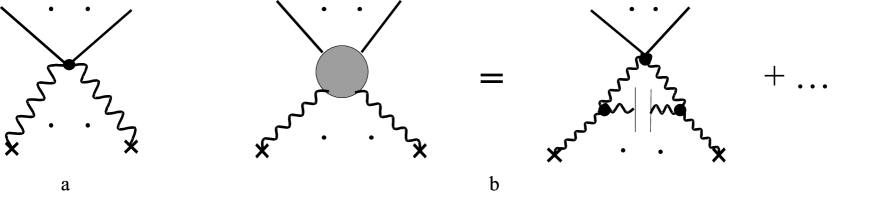
Figure 1: A typical vertex representing local interaction of the measuring device (straight lines) with the effective gauge field (wavy lines) in the standard interpretation (a). The corresponding non local vertex (the shaded blob) given by the generating functional (8) (b). The plus sign denotes higher-order contributions. The source $J$ for the gauge field is pictured schematically as the local crossed vertex.

Diagrammatically, this situation is illustrated in Fig.1. Fig.1(a) represents a typical vertex of the gauge field-device interaction according to the standard definition of the effective field as the quantum average of the corresponding field operator. It is implied by this definition that the mean field is simply put into the classical equations of device motion instead of its tree value. Such vertices are local, unlike those given by the generating functional (8) and represented in Fig.1(b). To determine effective equations of device motion we have to consider the sum of diagrams like that pictured in Fig.1(b), each having only one insertion of a $\phi$-vertex, since the device action is supposed to be infinitely small.

Now, introducing the generating functional of the connected Green functions

$$W(J)=-i~{}ln~{}Z(J),$$ (9)

we define the effective action $\Gamma$ as the Legendre transform of $W$ with respect to the mean gauge field

$$A_{a}=\frac{\delta W}{\delta J_{a}}$$ (10)

(denoted by the same symbol as the corresponding field operator):

$$\left.\Gamma(A)=W(J)-J_{a}A_{a}\right|_{J\to J(A)},$$ (11)

where the function $J(A)$ is implicitly defined by Eq. (10).

In the standard interpretation the reciprocal of Eq. (10)

$$\frac{\delta\Gamma}{\delta A_{a}}=-J_{a}$$ (12)

are the effective equations of motion for the full quantum corrected field $A$ corresponding to the given background field configuration $A^{0}$ satisfying

$$\frac{\delta S}{\delta A_{a}}(A^{0})=-J_{a}.$$ (13)

The use of $J$ as the source for the field $A^{0}$ instead of realistic matter sources, though formal, allows to simplify the derivation of the Slavnov identities below. As always, the source $J$ satisfies the ”conservation law”

$$D_{a\alpha}(A^{0})J_{a}=0,$$

where $A^{0}$ is the solution of Eq. (13), satisfying

$$F_{\alpha}(A^{0})=0.$$ (14)

3 The Slavnov identities

3.1 Preliminaries

Being a classical object the measuring device is completely described by its action. We can therefore investigate the gauge dependence of the latter rather than of the corresponding equations of motion (as was done in [1]). The action for the measuring device is the part of $\Gamma$ containing the fields $\phi_{i}$. Its gauge dependence is determined by the Slavnov identities for the generating functional of proper vertices corresponding to (8). However, these identities are complicated because of the peculiar role of the device action which is a kind of source for the gauge field. It is the nonlinearity of this source on the fields which complicates the usual derivation of the Slavnov identities.

Fortunately, in the present case we can limit ourselves by derivation of the Slavnov identities for the functional $W$ only. Indeed, the gauge dependent part of the device action is a sum of two different contributions. The first is the ordinary explicit gauge dependence of the effective action. The second results from implicit gauge dependence of the mean field $A$. Being a solution of the gauge dependent effective equations (12) the latter is also gauge dependent. It is precisely this gauge dependence of $A$ which lacks its physical interpretation. Thus, denoting by $\Gamma_{\phi}$ the part of $\Gamma$ containing $\phi$-fields we have for the full variation of the device action under a small change $\delta\xi$ of the gauge parameter $\xi$:

$$d\Gamma_{\phi}=\frac{\partial\Gamma_{\phi}}{\partial\xi}\delta\xi+\left.\frac{\delta\Gamma_{\phi}}{\delta A_{a}}\frac{\partial A_{a}}{\partial\xi}\right|_{J}\delta\xi\equiv\frac{d\Gamma_{\phi}}{d\xi}\delta\xi.$$ (15)

In (15) the derivative $\partial A_{a}/\partial\xi$ is calculated keeping $J$ fixed in accordance with the meaning of $J$ as producing the given classical field $A^{0}.$

Now note, that if we define the quantity $W_{\phi}$ by analogy with $\Gamma_{\phi}$, i.e., as the part of $W$ containing $\phi$, then

$$\Gamma_{\phi}(A)=\left.W_{\phi}(J)\right|_{J\to J(A)},$$ (16)

since the device action is supposed to be infinitely small.

Comparing (15) and (16) we arrive at the following important relation

$$\frac{d\Gamma_{\phi}(A,\xi)}{d\xi}=\left.\frac{\partial W_{\phi}(J,\xi)}{\partial\xi}\right|_{J\to J(A)}.$$ (17)

Thus, perhaps needed in carrying out the renormalization program, the Slavnov identities for $\Gamma$ turn out to be unnecessary in our consideration.

Let us now go over to the successive derivation of the Slavnov identities for $W.$

3.2 Derivation

Following the standard procedure (see, e.g., [6]) we perform a BRST shift (2) of integration variables in (8). Unlike the usual case, however, the quantum action (6) is not invariant under this operation, since besides the quantum fields $A,C,\bar{C}$ it contains the classical field $\phi$ which is not integrated in (8). Therefore, we obtain the following identity

$${\displaystyle\int}dAdCd\bar{C}\left[\frac{\delta S_{\phi}}{\delta A_{a}}D_{a\alpha}C_{\alpha}+J_{a}D_{a\alpha}C_{\alpha}+Y\bar{C}_{\alpha}F_{\alpha,a}D_{a\alpha}C_{\alpha}-\tilde{K}_{i}\tilde{D}_{i\alpha}f_{\alpha\beta\gamma}C_{\beta}C_{\gamma}-\frac{Y}{\xi}F_{\alpha}^{2}\right]\times$$

$$exp\{i(\Sigma(A,\phi,C,\bar{C},K,\tilde{K})+YF_{\alpha}\bar{C}_{\alpha}+J_{a}A_{a})\}=0,$$ (18)

where $S_{\phi}$ is the classical device action.

Since $S_{\phi}(A,\phi)$ is invariant under BRST transformations (2), we may write

$$\frac{\delta S_{\phi}}{\delta A_{a}}D_{a\alpha}(A)C_{\alpha}=-\frac{\delta S_{\phi}}{\delta\phi_{i}}\tilde{D}_{i\alpha}(\phi)C_{\alpha}.$$ (19)

Then the first term in square brackets in the left hand side of (3.2) can be transformed as

$${\displaystyle\int}dAdCd\bar{C}\frac{\delta S_{\phi}}{\delta A_{a}}D_{a\alpha}(A)C_{\alpha}exp\{...\}=-{\displaystyle\int}dAdCd\bar{C}\frac{\delta S_{\phi}}{\delta\phi_{i}}\tilde{D}_{i\alpha}(\phi)C_{\alpha}exp\{...\}$$

$$=-\frac{1}{i}\frac{\delta}{\delta\phi_{i}}{\displaystyle\int}dAdCd\bar{C}\tilde{D}_{i\alpha}(\phi)C_{\alpha}exp\{...\}+{\displaystyle\int}dAdCd\bar{C}\tilde{D}_{i\alpha}(\phi)C_{\alpha}\tilde{K}_{l}\frac{\delta\tilde{D}_{l\beta}(\phi)}{\delta\phi_{i}}C_{\beta}exp\{...\}$$

$$=\frac{\delta^{2}Z}{\delta\phi_{i}\delta\tilde{K}_{i}}+{\displaystyle\int}dAdCd\bar{C}\tilde{K}_{i}\tilde{D}_{i\gamma}(\phi)f_{\gamma\alpha\beta}C_{\alpha}C_{\beta}exp\{...\},$$ (20)

where locality of generators $\tilde{D}(\phi)$, and the property $\delta(0)=0$ were taken into account. The latter also implies that the third term in square brackets in (3.2) is equal to zero. Indeed, performing a shift $\bar{C}\to\bar{C}+\delta\bar{C}$ of integration variables in the functional integral (8) we obtain the quantum ghost equation of motion

$${\displaystyle\int}dAdCd\bar{C}\left[F_{\alpha,a}D_{a\beta}(A)C_{\beta}-YF_{\alpha}\right]exp\{...\}=0,$$ (21)

from which follows that

$$Y{\displaystyle\int}dAdCd\bar{C}\left[\bar{C}_{\alpha}F_{\alpha,a}D_{a\beta}(A)C_{\beta}-N\delta(0)\right]exp\{...\}=0.$$ (22)

Thus, the identity (3.2) can be rewritten as

$$\left(J_{a}\frac{\delta}{\delta K_{a}}+i\frac{\delta^{2}}{\delta\phi_{i}\delta\tilde{K}_{i}}-2Y\xi\frac{\partial}{\partial\xi}\right)Z=0.$$ (23)

This is the sought identity for the generating functional of the Green functions. It can be called effective Slavnov identity, since it is obtained under certain conditions concerning the device motion. In terms of the functional $W$ it looks like

$$J_{a}\frac{\delta W}{\delta K_{a}}-\frac{\delta W}{\delta\phi_{i}}\frac{\delta W}{\delta\tilde{K}_{i}}+i\frac{\delta^{2}W}{\delta\phi_{i}\delta\tilde{K}_{i}}=2Y\xi\frac{\partial W}{\partial\xi}.$$ (24)

In the next section (24) will be used to prove the low-energy gauge independence of the effective device action.

4 The gauge dependence cancellation

4.1 The renormalization equation

Definition of the device as a classical object, reflected in the way its action is introduced into the generating functional $Z,$ implies certain conditions under which the device motion can be considered in such a way, namely, it corresponds to the effective description of the device motion at low energies. Well known [3, 7], that in this case the leading quantum contribution to EA is due to non-analytical terms in the amplitudes, containing the logarithms of external momenta. On the other hand, the form of the latter can be simply read off from divergent parts of the amplitudes, since it is propagation of massless particles of the theory, which dominates at low energies (see, e.g., [3, 8]). For example, in the case of dimensionally regularized Feynman integrals of the type

$$\mu^{\varepsilon}{\displaystyle\int}d^{4-\varepsilon}qf(q,p_{1},...,p_{n}),$$ (25)

where $\varepsilon$ – dimensional regulator, $\mu$ – mass scale, and $f(q,p_{1},...,p_{n})$ – the result of all subintegrations, the low-energy leading contributions, corresponding to some powers of the logarithms of the external momenta $p_{1},...,p_{n}$, are given by zero order terms in the Loran expansion for (25) in powers of $\varepsilon$, and unambiguously determined by the poles of (25).

Thus, to determine the full gauge dependence of the device effective action, it is sufficient, in view of the relation (17), to investigate that of the divergent parts ($W^{div}$) of the generating functional $W$.

To do this, we use the Slavnov identity (24) to obtain the renormalization equation for $W^{div}.$ Namely, we first separate the $Y$-dependent part of $W$

$$W=W_{1}+YW_{2},$$

and substitute it in (24). Comparing multiples of $Y$ from the left and right hand sides of this identity then gives

$$2\xi\frac{\partial W_{1}}{\partial\xi}=-J_{a}\frac{\delta W_{2}}{\delta K_{a}}+\frac{\delta W_{1}}{\delta\phi_{i}}\frac{\delta W_{2}}{\delta\tilde{K}_{i}}-i\frac{\delta^{2}W_{2}}{\delta\phi_{i}\delta\tilde{K}_{i}},$$ (26)

where all the sources except $J_{a}$ are set equal to zero after differentiation.

Next, we extract the $\phi$-dependent part of (26) and obtain the following identity

$$2\xi\frac{\partial W_{1\phi}}{\partial\xi}=-J_{a}\frac{\delta W_{2\phi}}{\delta K_{a}}+\frac{\delta W_{1\phi}}{\delta\phi_{i}}\frac{\delta W_{2\bar{\phi}}}{\delta\tilde{K}_{i}}-i\frac{\delta^{2}W_{2\phi}}{\delta\phi_{i}\delta\tilde{K}_{i}},$$ (27)

where the symbol $W_{2\bar{\phi}}$ denotes the part of $W_{2}$ independent of the gauge field-device interaction. All of these identities are derived for invariantly regularized, but still unrenormalized functionals. Being connected with the high-energy behavior of the Green functions the renormalization of EA is immaterial in determination of the low-energy quantum corrections to the device motion. On the other hand, since we use the formal correspondence between divergences of EA and the form of logs in reconstruction of the leading quantum contributions to $\Gamma_{\phi},$ the effect of renormalization on the structure of divergences might seem to be important for us. However, as we have mentioned above, the use of the generating functional of the Green functions in the form of Eq. (8) is justified only in the low-energy regime of the device motion. Instead, the renormalization of the theory must be carried out, of course, in terms of the ordinary generating functional for which Eq. (8) is just an effective expression, and in which all the fields, including those corresponding to the measuring device, are considered as quantum. Thus, at each given order of the loop expansion it has to be supposed that all the subdivergences of the Green functions have been eliminated at lower orders according to the standard procedure, so that the only superficially divergent diagrams are in rest. It is the general result of the renormalization theory [4, 6] that this procedure can be arranged in the way that preserves the symmetry properties of the generating functionals of the Green functions. Thus, we suppose that the functional $W$ renormalized, say, up to $(n-1)$ th-loop order, satisfies the identity (27) and has local divergences of order $n.$

As follows from Eq. (17) divergences of $\partial W_{1\phi}/\partial\xi$ are to be determined after the substitution $J\to J(A)$ has been made. As always, this means that the corresponding one-particle-irreducible diagrams should be considered only. In the present case, however, one may substitute $J\to J(A^{0})$ directly, the function $J(A^{0})$ being determined by Eq. (13). Indeed, additional divergences associated with the reexpressing of the right hand side of Eq. (27) in terms of the mean field $A$, can appear, by assumption, only in the $n$ th-loop order. However, they actually do not contribute at this order, since the right hand side of Eq. (27) vanishes at the zeroth order, as one can easily verify.

Thus, splitting $W_{\phi}$ into the sum of divergent and convergent parts

$$W_{\phi}=W_{\phi}^{div(n)}+W_{\phi}^{con},$$

and noting that the corresponding parts of the identity (27) must cancel independently, we obtain the renormalization equation for $W_{\phi}^{div(n)}$:

$$2\xi\frac{\partial W_{1\phi}^{div(n)}}{\partial\xi}=-J_{a}\frac{\delta W_{2\phi}^{div(n)}}{\delta K_{a}}+\frac{\delta W_{1\phi}^{div(n)}}{\delta\phi_{i}}\frac{\delta W_{2\bar{\phi}}^{(0)}}{\delta\tilde{K}_{i}}+\frac{\delta W_{1\phi}^{(0)}}{\delta\phi_{i}}\frac{\delta W_{2\bar{\phi}}^{div(n)}}{\delta\tilde{K}_{i}},$$ (28)

where the superscript $(0)$ denotes the zeroth order approximation.

Let us now turn to examination of the right hand side of Eq. (28).

4.2 The power counting

We begin with definition of vertices and field propagators in the loop expansion. According to the standard procedure, one expands the exponent of the integrand in Eq. (8) around the extremal $A^{0}$

$$\Sigma(A,\phi,C,\bar{C},K,\tilde{K})+YF_{\alpha}\bar{C}_{\alpha}+J_{a}A_{a}=\Sigma(A^{0},\phi,C,\bar{C},K,\tilde{K})+J_{a}A^{0}+K_{a}D_{a\alpha}(A^{0})C_{\alpha}$$

$$+\tilde{K}_{i}\tilde{D}_{i\alpha}(\phi)C_{\alpha}+\frac{1}{2}\left(S+S_{gf}\right)_{,ab}(A^{0},\phi)a_{a}a_{b}+YF_{\alpha}(a)\bar{C}_{\alpha}+K_{a}D_{a\alpha,b}(A^{0})a_{b}C_{\alpha}+\cdot\cdot\cdot~{},$$

where the ellipsis denote terms of cubic and higher order in the quantum fields $a\equiv A-A^{0},~{}C,~{}\bar{C}.$ Note that in view of Eq. (14) the term $YF_{\alpha}(A^{0})\bar{C}_{\alpha}$ is absent in this expansion. Therefore, the second term in the right hand side of Eq. (28) vanishes identically.

For further examination of Eq. (28) it is necessary to employ the dimensional analysis. At this point we have to limit our general consideration and require the theory to be power-counting-renormalizable. Although quantum consequences of the original gauge symmetry of the classical action are normally expressed in the same form (like that of Eq. (28)) at all orders of the loop expansion even despite possible deformations of the gauge algebra, the strength of divergences of Feynman diagrams varies from order to order, in general. However, it is a common feature of all power-counting-renormalizable gauge theories that the degree of divergence $D$ of an arbitrary diagram with a set $\{n_{F}\}$ of external lines, where $\{F\}=\{A^{0},Y,K,\tilde{K}\}$, is less than or equals to

$$\tilde{D}\equiv 4-2n_{K}-2n_{\tilde{K}}-(2-\sigma)n_{Y}-\sigma n_{A^{0}},$$ (29)

$\sigma$ being the canonical dimension of the gauge field $a.$ The case $D<\tilde{D}$ corresponds to theories with superrenormalizable interactions.

It can be inferred from Eq. (29) that in the case of $\sigma=1$ (e.g., Yang-Mills theories) the third term in the right hand side of Eq. (28) is zero. Indeed, the only divergent diagram with $n_{\tilde{K}}=n_{Y}=1$ in this case corresponds to $n_{A^{0}}=1,$ and turns into zero, since the ghost vertex connected with the external $\tilde{K}$-line by the ghost propagator, contains the gauge condition operator $F_{\alpha,a}$ which vanishes upon acting on the rest of the diagram. This is illustrated in Fig.2.

Figure 2: Graphical representation of the third term in the right hand side of Eq. (28). Dashed lines correspond to FP ghost propagator $G$.

As far as the case $\sigma=0$ is concerned (e.g., $R^{2}$-gravity), there is an infinite number of logarithmically divergent diagrams with $n_{\tilde{K}}=n_{Y}=1$ and arbitrary number of external gauge fields. In this case the above argument goes if we confine ourselves by calculation of the gauge invariant part of the device action only.

Finally, from (29) follows that if the $\phi$-vertex were absent, then the remaining term in the right hand side of Eq. (28) would diverge, with $\tilde{D}=\sigma$. Whether it does depends on the form of the device-gauge field interaction. Obviously, insertion of a vertex corresponding to this interaction makes a diagram with $\tilde{D}=\sigma$ convergent if and only if

$$N_{\partial}+\sigma N_{a}<4-\sigma,$$ (30)

where $N_{a},N_{\partial}$ are numbers of the gauge fields entering the vertex, and acting on them derivatives, respectively. This condition is obviously satisfied if the full underlying quantum theory of interacting gauge and matter fields is also power-counting renormalizable.

Summing up, the right hand side of Eq. (28) turns out to be zero, thus proving gauge independence of the low-energy effective action of the measuring device.

5 Discussion and Conclusion.

We have shown that in the case when the quantum propagation of the fields describing measuring device can be neglected, namely, in the low-energy classical limit, the effective equations of device motion turn out to be gauge independent at any order of the loop expansion.

This allows to define in the same limit the gauge independent effective gauge field as the field that enters these equations and couples to the measuring device in the classical fashion. We would like to emphasize that it is purely classical nature of the observables (which are functionals of the $\phi$-fields) due to which the well-known problem of their unambiguous definition [10, 11] does not arise in our consideration. So, whether it is possible to extend the definition to higher energies depends on eventual applicability of the classical conceptions contained in the notion of measurement.

Now, turning back to the item 3. of the Introduction, it is natural to ask whether the value of the effective gauge field, defined in the manner described above, is one and the same for all measuring devices. It definitely is in the case of infinitesimal device action, considered above. Indeed, in this case account of any possible dependence of the effective gauge field on characteristics of the measuring device would exceed the precision chosen in our discussion. It is not clear, however, whether this is true in the general case of finite disturbances produced in the effective field by the process of measurement.

References

- [1] D. Dalvit and F. Mazzitelli, Phys.Rev. D56 n.12 (1997) 7779.
- [2] C. Becchi, A. Rouet and R. Stora, Ann. of Phys. 98 (1976) 287; Commun. Math. Phys. 42 (1975) 127; I. V. Tyutin, Report FIAN 39 (1975).
- [3] J. F. Donoghue, Phys.Rev. D50 n.6 (1994) 3874.
- [4] P. M. Lavrov, I. V. Tyutin and B. L. Voronov, Yad. Fiz. v.36 (1982) 498 [Sov. Journ. Nucl. Phys. v.36 (1982) 292].
- [5] H. Kluberg-Stern and J. B. Zuber, Phys. Rev. D 12 (1975) 467, 3159; N. K. Nielsen, Nucl. Phys. B101 (1975) 173; D. Johnston, Nucl. Phys. B293 (1987) 229; C. M. Fraser and I. J. R. Aitchison, Ann. of Phys. (N.Y.) 156 (1984) 1; O. Piguet and K. Sibold, Nucl. Phys. B253 (1985) 517.
- [6] J. Zinn-Justin, Renormalization of gauge theories, in: Trends in elementary particle physics, edited by H. Rollnik and K. Dietz (Springer-Verlag, Berlin, 1975) p. 2.
- [7] S. Weinberg, Physica (Amsterdam) 96A (1979) 327; J. F. Donoghue, in: Effective Field Theories of the Standard Model, edited by U.-G. Meissner (World Scientific, Singapore, 1994); H. Leutwyler and S. Weinberg, in Proceedings of the XXVIth International Conference on High Energy Physics, edited by J. Sanford (Dallas, Texas, 1992), AIP Conf. Proc. No. 272 (AIP, NY, 1993) pp. 185, 346.
- [8] G. A. Vilkovisky, The gospel according to DeWitt, in: Quantum theory of gravity, edited by S. M. Christensen (Hilger, Bristol, 1984) p. 169.
- [9] K. A. Kazakov and P. I. Pronin, Phys. Rev. D 59 (1999) 064012.
- [10] B. S. DeWitt, The quantization of geometry, in: Gravitation: an introduction to current research, edited by L. Witten (Wiley, New-York, 1962) p. 266.
- [11] G. A. Vilkovisky, Nucl. Phys. B234 (1984) 125; Class. Quantum Grav. 9 (1992) 895.