FTUAM-99-13; IFT-UAM/CSIC-99-19 INLO-PUB-9/99

Abstract: We give a unified description of self-dual $SU(2)$ gauge fields on tori of size $\l_{t}\times l_{s}^{3}$, based on a mixture of analytical and numerical methods using the Nahm transformation, extended to the case of twisted boundary conditions. We show how torus calorons ($l_{t}/l_{s}$ small) are Nahm dual to the torus instantons ($l_{t}/l_{s}$ large). Holonomies are dual to the locations of constituents, this duality becoming exact in the limiting cases $l_{s}$ or $l_{t}\rightarrow\infty$. Implications for the moduli spaces are discussed.

1 Introduction

The study of $SU(N)$ gauge fields on the torus has a long history (see Ref. [1] for a recent account). It was initiated by G. ‘t Hooft [2] who pointed out additional non-trivial topological features, associated to what is known as twisted boundary conditions (tbc), describing the presence of center-valued conserved fluxes for non-abelian gauge fields. In particular, the study of self-dual gauge field configurations on the torus has become a challenging problem. Both within the finite volume Hamiltonian and the finite temperature formulations of non-abelian gauge theories they play an important role, and the main result of this paper is a rather surprising detailed dual relationship between these solutions.

For non-zero twist, numerical methods based on the lattice formulation of gauge theories strongly suggested the existence of non-abelian self-dual solutions for all torus sizes [3, 4]. Indeed, existence of smooth solutions with one unit of topological charge ($Q$) and any non-trivial twist has been established rigorously [5], even though one can prove non-existence for zero twist [6]. (For higher topological charges existence has been proven by Taubes [7] earlier). To date, however, no analytic expressions have been found for these non-abelian solutions on the 4-torus. This contrasts with the situation for $R^{4}$ (or $S^{4}$), where one has the algebraic ADHM construction [8].

An important technique for studying self-dual gauge fields is the Nahm transformation [9], which is particularly simple for the torus. It maps $SU(N)$ self-dual solutions of charge $Q$ on the torus to $SU(Q)$ self-dual solutions of charge $N$ on the dual torus. The mapping is an involution, i.e. applying the Nahm transformation again brings one back to the original gauge field configuration. The only analytically known example of the Nahm transformation on the torus, based on a particular abelian solution [10], maps it onto itself [11]. Nevertheless, the Nahm transformation is believed to be an important ingredient in leading to analytical results for the self-dual solutions.

A few strategies have been used to improve our understanding of this problem. One follows from the consideration of mixed compact and non-compact directions $T^{n}\times R^{4-n}$. Under the duality transformation the non-compact directions collapse and the dual space is an $n$-dimensional torus, thereby achieving a dimensional reduction. The most dramatic example is that of $n=0$, where the dual space collapses to a point, being the reason that the ADHM construction [8] is algebraic. The $n=1$ case is relevant at finite temperature [12, 13] for which the associated geometry is $R^{3}\times S^{1}$. The case $n=3$ was considered as a way to circumvent the no-go theorem on $Q=1$, zero-twist configurations [14, 15]. This geometry is relevant for the Hamiltonian formulation of gauge fields on the spatial torus, with the non-compact direction identified with time. The possibility of having $Q=1$ configurations introduces an important additional simplification, since its Nahm-dual connection is an abelian gauge field.

Applying Nahm’s transformation in the non-compact case demands some modifications [11]. In particular, there appear a finite number of singularities where the Nahm transformed gauge field is non-selfdual. These occur when the holonomy of the original self-dual gauge field (extended to $U(N)$ by adding a curvature free abelian gauge field, which parametrises the coordinates of the dual torus) has a trivial eigenvalue. The holonomy is defined by the Wilson loops winding non-trivially in the compact directions, when taken to infinity in the non-compact directions.

An important example of the appearance of these singularities in the Nahm transformation is the case of calorons [12, 13], instantons at finite temperature. It was already known from the early work of Nahm [9] that the dual formulation involves a $U(1)$ gauge field on the circle with suitable singularities. It was only recently that explicit expressions for the $Q=1$ self-dual configurations on $R^{3}\times S^{1}$ with non-trivial holonomy were obtained [16, 17]. In particular it was shown how the location of the singularities in the dual field is related to the holonomy (the Polyakov loop at spatial infinity). These non-trivial calorons reveal the presence of constituent BPS monopoles, hidden at trivial holonomy due the masslessness of one of the monopoles.

Another example recently analysed in detail is the $Q=1$ instanton configuration for $T^{3}\times R$ with twisted boundary conditions in time [18]. There the location of the singularities is determined by the holonomies (Polyakov loops in the three directions of $T^{3}$) at infinite time. Away from these singularities, the abelian Nahm transformed field is self-dual and therefore satisfies Maxwell equations. The singularities act as sources and can be interpreted as point-like dyons carrying (equal) electric and magnetic charge.

It is interesting to ask oneself how these caloron and instanton configurations are approached from configurations on a torus, $l_{t}\times l_{s}^{3}$, when sending either $l_{s}$ or $l_{t}$ to infinity. When finite, these configurations will be referred to as torus calorons and torus instantons respectively. Both types of configurations have been analysed in the past by means of numerical methods. In [14] it was seen how some of the $T^{3}\times R$ configurations are the limit of self-dual configurations on the 4-torus with twisted boundary conditions in time, which are known to exist [5]. The $Q=1$ solution tunnels between vacua where some of the holonomies have opposite signs. The non-existence of the $Q=1$ solution without twist was understood as an obstruction for tunnelling between two vacua with the same holonomy. The situation seems quite similar to the O(3) model on the cylinder, which turned out to be tractable analytically [19].

The case of non-zero spatial twist was studied numerically even earlier. The basic building block is a lump –the twisted instanton– carrying fractional topological charge ($Q={\scriptstyle{{1\over 2}}}$ for $SU(2)$) and which is well localised in time [3, 4, 20]. Single twisted instanton configurations arise for non-zero (so called non-orthogonal) twist, both in space and time, and they have a well-defined limit as $l_{t}\rightarrow\infty$. Only their overall position is a free parameter, so that in particular their scale is fixed (to $l_{s}$). Higher topological charge configurations look as superpositions of these twisted instantons, distributed in the time-direction [21, 22]. These $Q={\scriptstyle{{1\over 2}}}$ lumps also feature prominently in numerical studies that address how 4-torus configurations approach the non-compact geometries of $T^{2}\times R^{2}$ [23].

Finally, caloron configurations on a torus have been recently studied [24] on lattices typically having $l_{s}/l_{t}=4$ or higher. These torus calorons fitted extremely well to the infinite volume analytic results. Interestingly, twist in the time direction enforces the holonomy (when taking the limit $l_{s}\rightarrow\infty$) to have zero trace, which implies the constituent monopoles of the caloron have equal mass. For spatial twists, however, the numerical analysis of Ref. [24] suggests that the constituent monopoles are forced to sit at fixed relative positions on the torus, but can have arbitrary masses (only constrained by the total topological charge). One can also study one constituent monopole in isolation by having suitable twists, both in space and time, such that it supports the $Q={\scriptstyle{{1\over 2}}}$ twisted instanton mentioned before. Indeed in the limit $l_{t}/l_{s}\rightarrow 0$ this solution becomes time independent and thus has to approach a single BPS monopole. Hence also in this limit the twisted instanton - as the BPS monopole - is the basic building block, but now arbitrarily placed in space.

Quite remarkably, as will be discussed in this paper, torus calorons are dual to torus instantons, with either their space (for calorons) or time (for instantons) positions determined by the holonomies of their Nahm dual. In the limit $l_{t}\rightarrow\infty$, relevant for $T^{3}\times R$, the Nahm dual has the limit $\hat{l}_{t}\rightarrow 0$ (setting $l_{s}=1=1/l_{s}$ for convenience). This means that the non-abelian cores of the torus caloron shrink to zero and one is left with the abelian field discussed before. Quite in the same way one can interpret the abelian dual of the caloron in the limit $l_{s}\rightarrow\infty$ (here setting units by $l_{t}=1$, the Nahm dual has $\hat{l}_{s}\rightarrow 0$) as the limit in which the instanton cores have shrunk to zero. In both cases the non-abelian field is self-dual at all values of $l_{t}$ and $l_{s}$, and the violation of the abelian self-duality in the limiting case is thus due to ignoring the singular non-abelian cores of the constituents. Such understanding of the singularity may prove important for future analytic work in the $T^{3}\times R$ case.

In our analysis, two ingredients play an important part. One is that for $T^{4}$ lattice techniques have been developed [25] that allow us to study the Nahm transformation numerically. This was tested in a non-trivial example for $SU(2)$ with charge 2, which maps to itself. This demonstrated that the method is precise enough to become a useful tool in numerically analysing the properties of the Nahm dualities. This charge 2 configuration was actually composed from four $Q={\scriptstyle{{1\over 2}}}$ twisted instantons. As we will see, it is these twisted instantons that are mapped on to themselves as they only have their position as a free parameter.

The other ingredient is the recent formulation of the Nahm transformation in the presence of twisted boundary conditions [26]. The Nahm transform of an $SU(N)$, charge $Q$ self-dual configuration is an $SU(N_{0}Q)$ configuration with topological charge $\hat{Q}=N/N_{0}$, where $N_{0}$ is an integer depending on the twist. If the original twist is non-trivial the Nahm transform lives on a torus with non trivial twist. In essence the construction is related to recognising twist as (for $SU(2)$) half-periods for a larger torus, to which the usual Nahm transformation can be applied. Remarkably, the dual configuration admits “half-periods” as well, and the dual gauge field can thus be formulated in terms of gauge fields with twisted boundary conditions. It is this that allows us to demonstrate that the $Q={\scriptstyle{{1\over 2}}}$ $SU(2)$ twisted instanton is mapped to itself under the Nahm transformation.

Alternative to the formulation in terms of “doubling”, one can introduce a suitable flavour group to compensate for the twist [27], with which the Nahm transformation can then be performed. Again one might study half-periods in the resulting dual torus and reach a self-dual configuration in a smaller torus (the Nahm-dual torus) and with non-zero twist (the Nahm-dual twist) [26]. Furthermore, it was shown that both formulations agree. From the analytical point of view this method is more general and allows a simple and compact characterisation of the Nahm-dual torus and twist. This will be presented in an Appendix.

In this paper we will make a synthesis of all the results mentioned above, leading to additional insight in self-dual gauge fields on the torus and their moduli spaces. In Section 2 we will set up the formalism, whereas section 3 shows how the torus calorons and torus instantons are related under the Nahm transformation, illustrated explicitly by numerical examples. We show that taking the appropriate limits, as discussed qualitatively in this introduction, reproduces the known analytic results.

2 The Nahm transformation with twist

Let us consider a 4 dimensional torus. This can be defined as $R^{4}/\Lambda$ where $\Lambda$ is a rank-four lattice of points. Let $e^{(\alpha)}$ stand for four vectors ($\alpha\in\{0,1,2,3\}$) which can be chosen as generators of $\Lambda$. We will take in general a hypercubic torus $l_{t}\times l_{1}\times l_{2}\times l_{3}$, for which $e^{(0)}=(l_{t},0,0,0)$, $e^{(1)}=(0,l_{1},0,0)$, $e^{(2)}=(0,0,l_{2},0)$ and $e^{(3)}=(0,0,0,l_{3})$. Often we will take $l_{1}=l_{2}=l_{3}\equiv l_{s}$. For obvious physical reasons we will refer to the direction with length $l_{t}$ as time and to the other three as space.

Now consider $SU(N)$ self-dual gauge fields $A_{\mu}(x)$ defined on this torus. They can be looked at as fields defined on $R^{4}$, periodic modulo gauge transformations under translations by vectors $a$ in the lattice $\Lambda$. Given any element of $\Lambda$, $a\equiv e(s)=s_{\alpha}e^{(\alpha)}$ ($s_{\alpha}\in Z$), we have (our convention throughout this paper is that $A_{\mu}(x)$ is hermitian)

$$A_{\nu}(x+a)=[\Omega_{a}]A_{\nu}(x)\equiv\Omega_{a}(x)\,A_{\nu}(x)\,\Omega^{\dagger}_{a}(x)+i\ \Omega_{a}(x)\,\partial_{\nu}\Omega^{\dagger}_{a}(x)\quad,$$ (1)

where $\Omega_{a}(x)$ form a family of $SU(N)$ matrices, known as twist matrices. Since the lattice $\Lambda$ is abelian, the matrices $\Omega_{a}(x)$ must satisfy the following consistency conditions

$$\Omega_{a}(x+b)\,\Omega_{b}(x)=e^{2\pi i{\cal N}(a,b)}\,\Omega_{b}(x+a)\,\Omega_{a}(x)\quad.$$ (2)

Because the matrices belong to $SU(N)$, the factor $\exp(2\pi i\,{\cal N}(a,b))$ must be an element of the center $Z_{N}$. Hence, ${\cal N}(a,b)$ is an antisymmetric bilinear form defined by its action on the generators

$${\cal N}(e^{(\alpha)},e^{(\beta)})=\frac{n_{\alpha\beta}}{N}\quad,$$ (3)

where $n_{\alpha\beta}$ is an antisymmetric matrix of integers defined modulo $N$, known as the twist tensor. We will frequently refer to its elements in the form of two 3-vectors of integers: $k_{i}=n_{0i}$ and $m_{i}={\scriptstyle{{1\over 2}}}\varepsilon_{ijk}n_{jk}$.

An important role in what follows will be played by the lattice $\Lambda_{0}$, a sublattice of $\Lambda$. This is given by the elements $a\in\Lambda$, such that the associated gauge transformation $\Omega_{a}(x)$ commutes (in the sense of the composition in Eq. (2)) with all other $\Omega_{b}(x)$. Equivalently

$$\Lambda_{0}\equiv\{a\in\Lambda\;|\;{\cal N}(a,b)\in Z,\quad\forall b\in\Lambda\}\quad.$$ (4)

The quotient group $\Lambda/\Lambda_{0}$ is a finite abelian group. Using the freedom to select a basis of $\Lambda$ such that $n_{\alpha\beta}$ has the canonical Frobenius form, one can show that the order of this group is the square of some integer, $N_{0}^{2}$. The integer $N_{0}$ plays an important role in what follows and depends only on the form ${\cal N}$. It is clear that for trivial twist vectors $\vec{k}=\vec{m}=\vec{0}\bmod N$ (${\cal N}(a,b)\in Z$) one has $\Lambda_{0}=\Lambda$ and $N_{0}=1$.

Now let us proceed to introduce Nahm’s transformation [9, 6]. For that purpose add a 4 parameter family of curvature free abelian gauge fields to the original self-dual gauge field, $A_{\mu}(x)+2\pi z_{\mu}I$. This family of $U(N)$ gauge fields is still self-dual, as the curvature is not affected by the addition. The zero-modes of the Weyl equation in this background satisfy

$$(\overline{D}-2\pi i\bar{z})\Psi_{z}^{\alpha}(x)=0\quad.$$ (5)

In this notation we associate to each four-vector $C_{\mu}$ a $2\times 2$ matrix $\overline{C}=C_{0}\,I_{2\times 2}+i\vec{C}\cdot\vec{\sigma}$ (with $\sigma_{k}$ the Pauli matrices). The covariant derivative $D_{\mu}$ is given by $\partial_{\mu}-iA_{\mu}(x)$. In the absence of twist ($\vec{k}=\vec{m}=0$), the Weyl spinors satisfy the boundary conditions:

$$\Psi_{z}^{\alpha}(x+a)=\Omega_{a}(x)\Psi_{z}^{\alpha}(x)\quad,$$ (6)

and the index theorem [28] implies that the number of solutions satisfying Eqs. (5-6) (labelled by $\alpha$) is given by the topological charge $Q$. Then the Nahm transformed gauge field is given by

$$\hat{A}_{\mu}^{\alpha\beta}(z)=i\int d^{4}x\,\Psi_{z}^{\alpha}(x)^{\dagger}\frac{\partial}{\partial z_{\mu}}\Psi_{z}^{\beta}(x)\quad.$$ (7)

Quite miraculously this is an $SU(Q)$ self-dual gauge field with topological charge $N$. Furthermore, the gauge field is defined on a dual torus $\tilde{R}^{4}/\tilde{\Lambda}$, where $\tilde{\Lambda}$ is the dual lattice of $\Lambda$.

With non-trivial twist ($\vec{k},\vec{m}\neq 0$) the boundary conditions shown in Eq. (6) are no longer valid, since $\Psi_{z}^{\alpha}(x)$ takes values in the fundamental representation of $SU(N)$, which transforms non-trivially under the center of the gauge group. Two strategies were developed in Ref. [26] to deal with this. One involves adding flavour and the other replicating the original torus. Both methods were shown to lead to the same Nahm transformed gauge field.

For the flavour construction one introduces the $U(N_{f}N)$ self-dual gauge field $A_{\mu}(x)\otimes\,I_{N_{f}\times N_{f}}$. The enlargement of the colour space allows us to modify the twist matrices as follows: $\Omega_{a}(x)\rightarrow\Omega_{a}(x)\otimes\Gamma^{*}(a)$. The $N_{f}\times N_{f}$ constant matrices $\Gamma(a)$ satisfy

$$\Gamma(a)\,\Gamma(a^{\prime})=e^{2\pi i{\cal N}(a,a^{\prime})}\,\Gamma(a^{\prime})\,\Gamma(a)\quad.$$ (8)

In this way the new $U(N_{f}N)$ matrices $\Omega_{a}(x)$ have no twist, and the standard formalism can be applied to them. The existence of solutions to Eq. (8), known as twist-eaters, was studied in the past [33]. The constant matrices $\Gamma(a)$ are known to exist provided $N_{f}$ is a multiple of $N_{0}$, the twist-dependent integer defined below Eq. (4). The solutions form an irreducible set provided the matrices are precisely $N_{0}\times N_{0}$. Furthermore, the solution is unique modulo similarity transformations and multiplication by constants [33, 1]. If we restrict to matrices belonging to $U(N_{0})$ these constants are necessarily phases (a $U(1)$ representation of the lattice $\Lambda$). Hence, we will consider $N_{f}=N_{0}$ and make a particular choice of solutions $\Gamma(a)$. In the appendix we show how different choices of the twist eaters correspond to translations in $z$ of the Nahm transformed field.

We have reduced the problem to the situation without twist, for a $U(N_{0}N)$ self-dual gauge field defined on the torus $R^{4}/\Lambda$ with topological charge $\hat{N}=N_{0}Q$. One can then construct the Nahm transformed gauge field in the standard way. It will be a $U(\hat{N})$ self-dual gauge field with topological charge $N_{0}N$, living on the dual torus $R^{4}/\tilde{\Lambda}$. The construction is in terms of the solutions of the Weyl equation in the background of the $U(N_{0}N)$ gauge field (adding $2\pi z_{\mu}I$). However, given the tensor product form of this gauge field, these zero-modes are seen to be solutions of the original $U(N)$ Weyl equation (5). But the boundary condition, Eq. (6), is replaced by

$$\Psi_{z}^{i\alpha}(x+a)=\Omega_{a}(x)\,\Gamma_{ij}^{*}(a)\,\Psi_{z}^{j\alpha}(x)\quad,$$ (9)

where $i,j$ are flavour indices (taking $N_{0}$ values). The index theorem tells us that the label $\alpha$, running over the linearly independent solutions, takes $\hat{N}=N_{0}Q$ values. Choosing these solutions to form an orthonormal set, we can express the dual gauge field as follows:

$$\hat{A}_{\mu}^{\alpha\beta}(z)=i\sum_{i=1}^{N_{0}}\int d^{4}x\,\Psi_{z}^{i\alpha}(x)^{\dagger}\frac{\partial}{\partial z_{\mu}}\Psi_{z}^{i\beta}(x)\quad.$$ (10)

Although this field is in principle living on the torus $R^{4}/\tilde{\Lambda}$, in Ref. [26] it is shown that it possesses additional periodicities. Hence, one can define the Nahm transform of the original gauge field with non-trivial twist as the restriction of the gauge field given in Eq. (10) to the minimal torus, in which case it has non-trivial twist as well. It can be shown that this minimal torus is precisely $R^{4}/\hat{\Lambda}$, where $\hat{\Lambda}=\tilde{\Lambda}_{0}$, the dual lattice of $\Lambda_{0}$ (see Eq. (4)). This definition preserves the property that the Nahm transformation is an involution, and reduces to the standard construction for trivial twist. Proofs are given in Ref. [26]. A more elegant, basis independent derivation is given in the appendix.

Now we will explain briefly what is the essence of the alternative construction, which is directly related to our numerical implementation of the Nahm transform. We can view $A_{\mu}(x)$ on $R^{4}/\Lambda$ as being defined on the 4 dimensional hypercube formed by the unit cell (spanned by $e^{(\mu)}$) of $\Lambda$, with appropriated twisted boundary conditions. Consider now a sublattice $\Lambda^{\prime}$ whose unit cell is obtained by duplicating the original hypercube in various directions, in such a way that the net twist vanishes. So one defines $A_{\mu}(x)$ on $R^{4}/\Lambda^{\prime}$, such that its boundary conditions do no longer carry twist. A trivial way to achieve this is by taking $\Lambda^{\prime}=\Lambda_{0}$, whose unit cell contains $N_{0}^{2}$ unit cells of $\Lambda$, but this is not a minimal choice.

To determine $\Lambda^{\prime}$ it is simplest to make a choice of generators for $\Lambda$ such that $n_{\alpha\beta}$ takes the Frobenius standard form with non-zero entries defined by $n_{02}=-n_{20}=q_{1}$ and $n_{31}=-n_{13}=q_{2}$. We introduce $p_{1}$ and $p_{2}$ as the smallest positive integers such that $q_{i}p_{i}/N\in Z$. One duplicates the hypercube $(p_{1}-1)$ times in either the 0 or 2 direction and $(p_{2}-1)$ times in either the 1 or 3 direction such that $N_{0}=p_{1}p_{2}$. Further freedom arises in case $p_{i}$ has non-trivial prime factors. The new gauge field on $R^{4}/\Lambda^{\prime}$ has topological charge $N_{0}Q$ and no twist. Now one can apply the Nahm transformation, which maps to a $SU(N_{0}Q)$ self-dual gauge field of topological charge $N$, defined on $R^{4}/\tilde{\Lambda}^{\prime}$.

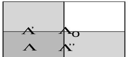
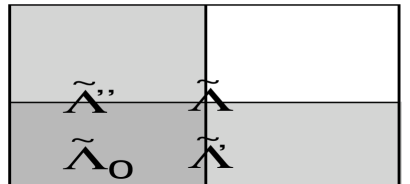
Figure 1: We present a cross section through the 0-2 plane of the various lattices that appear in the Nahm transformation with twisted boundary conditions $n_{02}=-n_{20}=1$ on $R^{4}/\Lambda$. Units are such that $l_{0}^{2}=l_{2}^{2}={\scriptstyle{{1\over 2}}}$, for which $R^{4}/\tilde{\Lambda}_{0}$ is of the same size as the original torus. In this case $N_{0}=2$ and the two choices for the minimal lattices with twist are denoted by $\Lambda^{\prime}$ and $\Lambda"$. The dual of the lattice $\Lambda_{0}$ gives the torus on which the Nahm transformed gauge field lives, with the same twist. Duplications on the dual side are identical, except for interchanging the roles of $\Lambda$ and $\Lambda_{0}$ (and less importantly $\Lambda^{\prime}$ and $\Lambda"$). When a symbol overlaps with different cells it belongs to all of those cells as a whole.

Each choice of $\Lambda^{\prime}$ will lead to a different set of zero-modes. This can only mean that the resulting dual gauge fields are related by gauge transformation. Gauge invariant quantities have to agree when derived from the various choices of $\Lambda^{\prime}$. But this means that the smallest unit cell in terms of which these gauge invariant quantities can be reproduced, is the intersection of the unit cells of all $\tilde{\Lambda}^{\prime}$, which is precisely $\hat{\Lambda}=\tilde{\Lambda}_{0}$, the dual of $\Lambda_{0}$ (in the same way the unit cell of $\Lambda$ is the intersection of the unit cells of all $\Lambda^{\prime}$). Note that $\Lambda_{0}$ is the smallest sublattice of $\Lambda$, that is also a sublattice of all possible choices of $\Lambda^{\prime}$ (the unit cell of $\Lambda_{0}$ consists of $N_{0}$ unit cells of $\Lambda^{\prime}$ and therefore of $N_{0}^{2}$ unit cells of $\Lambda$). With the twist in the standard form given above, $\Lambda_{0}$ is obtained by duplicating the hypercube that defines the original torus $R^{4}/\Lambda$, $(p_{1}-1)$ times in both the 0 and 2 directions and $(p_{2}-1)$ times in both the 1 and 3 directions. In Fig. 1 we elucidate this for the 0-2 plane with $q_{1}=1$ and $p_{1}=2$.

This shows that $\hat{A}$ can be defined as an $SU(N_{0}Q)$ gauge field on $R^{4}/\tilde{\Lambda}_{0}$ [26] and has topological charge $N/N_{0}$. Nevertheless, as is obvious in particular for $N/N_{0}$ not an integer, the unit cell of $\Lambda_{0}$ cannot be without twist, i.e. $\hat{A}$ is also a gauge field with twisted boundary conditions. For $SU(2)$ in the case that the original twist is already in the Frobenius standard form (where the situation of Fig. 1 applies in the 0-2 and/or the 1-3 planes), the dual twist can be read off from the minimal number of duplications required to go from $\tilde{\Lambda}_{0}$ to any of the choices $\tilde{\Lambda}^{\prime}$.

3 The case of $SU(2)$ (twisted) instantons

Having presented the general formalism, let us now concentrate on the study of $SU(2)$ gauge field configurations for spatially symmetric tori. From the previous formulas one can deduce that the symmetric structure of the torus is not always preserved by the Nahm transform. Nonetheless, the dual torus is always contained within the symmetric torus $R^{4}/\tilde{\Lambda}$. Furthermore, if a given torus has $l_{s}/l_{t}\gg 1$, its Nahm transform corresponds to $l_{s}/l_{t}\ll 1$. Thus, the Nahm transform of the torus instanton configurations are the torus caloron configurations. The space of gauge inequivalent solutions defines the moduli space. Its dimension is given through an index theorem to be $4NQ$ for $SU(N)$ gauge fields of charge $Q$ on the torus. Note that $QN=\hat{Q}\hat{N}$ so that the dimensionality is preserved by the Nahm transform. Indeed, in Ref. [6] it is proven that the Nahm transformation induces an isometry between the moduli spaces.

3.1 The twisted instanton $Q={\scriptstyle{{1\over 2}}}$

We start with the smallest value of the topological charge, for $SU(2)$ this is $Q={\scriptstyle{{1\over 2}}}$. The dimension of the moduli space is 4, so that the set of solutions is discrete up to translations. The value of the topological charge is related to the twist by the formula [2, 29]

$$Q=\nu-\frac{\vec{k}\cdot\vec{m}}{N}\quad,$$ (11)

where $\nu$ is an integer. Fractional values of the topological charge are attainable for non-orthogonal twists, i.e. $\vec{k}\cdot\vec{m}\neq 0\bmod N$. For $SU(2)$ we choose $\vec{k}=\vec{m}=(0,1,0)$, with $\vec{k}\cdot\vec{m}=1$. We deduce $N_{0}=4$ and therefore the Nahm transformation is again an $SU(2)$ self-dual gauge field with topological charge ${\scriptstyle{{1\over 2}}}$. Furthermore, it lives on a torus with generators $\hat{e}^{(\mu)}={\scriptstyle{{1\over 2}}}\tilde{e}^{(\mu)}$, where $\tilde{e}^{(\mu)}$ are the dual basis vectors $\tilde{e}^{(0)}=(1/l_{t},0,0,0)$, $\tilde{e}^{(1)}=(0,1/l_{s},0,0)$, $\tilde{e}^{(2)}=(0,0,1/l_{s},0)$, $\tilde{e}^{(3)}=(0,0,0,1/l_{s})$. The corresponding twist is unchanged.

Now we will explain how this works for configurations with $l_{s}/l_{t}\ll 1$. This will serve to illustrate the precision of our numerical techniques. One can generate self-dual configurations numerically by employing the method described in Ref. [3]. To minimise the errors due to lattice artifacts we actually make use of the improved cooling technique described in Ref. [14], with the parameter $\varepsilon=0$. One can implement twist by the method of Ref. [30]. We have generated self-dual configurations with the twist mentioned above on lattices of size $4\times 16^{3}$ and $32\times 8^{3}$. Notice that in the former case $l_{s}/l_{t}=4$ and in the latter case $\frac{1}{4}$. They correspond to Nahm-dual tori for this twist. In both cases the action density of the configuration has a lumpy profile with a single maximum in space. The position of the maximum does not coincide with a lattice point, but can be estimated by interpolation. Then, given the interpolated position of the maximum, one can determine the coordinates corresponding to each lattice point with respect to it.

Figure 2: Comparison between the action densities of a numerical $Q={\scriptstyle{{1\over 2}}}$ instanton with twist $\vec{k}=\vec{m}=(0,1,0)$, living on a $32\times 8^{3}$ lattice, and the Nahm transformation of a $Q={\scriptstyle{{1\over 2}}}$ caloron (BPS monopole) with the same twist, living on a $4\times 16^{3}$ lattice. The depicted values correspond to points in the $32\times 8^{3}$ lattice, along the lattice direction $\vec{n}_{latt}=(8,4,8)$; the peak of the action density of the lattice instanton being interpolated, in lattice coordinates, to $n=(15.809,3.741,3.979,4.162)$ and shifted to $({\scriptstyle{{1\over 4}}},{\scriptstyle{{1\over 16}}},{\scriptstyle 0},{\scriptstyle{{1\over 16}}})$ where the maximum of the Nahm transform of the caloron sits. The continuum time period has been set to $l_{t}=1$ for the caloron and hence $\tilde{l_{t}}={\scriptstyle{{1\over 2}}}$ for its Nahm transformed instanton.

What we did next was to apply the numerical Nahm transformation introduced in Ref. [25]. The values of $z$, where the Nahm transformation was calculated, were those corresponding to the lattice points of the dual configuration. In this way the Nahm transformation can be compared with the lattice configuration obtained on the dual torus. Fig. 2 shows the result of such a comparison for the action density along a line on the torus. The agreement is remarkable. It shows the way in which our expectations work and gives us confidence on the precision of our numerical methods to investigate other more complicated situations. Note that in fact Ref. [25] dealt with the case of four $Q={\scriptstyle{{1\over 2}}}$ instantons (with $l_{s}/l_{t}=1$) on a $12\times 6\times 12\times 6$ lattice, finding that the configuration is mapped to itself (up to a shift). In terms of the $Q={\scriptstyle{{1\over 2}}}$ twisted instantons this can be understood from the fact that only its position is a free parameter. Since the work in Ref. [25] the numerical methods have been greatly improved, details of which will be reported elsewhere.

3.2 Temporal twist $Q=1$

Let us recall what is known about $Q=1$ configurations with $\vec{m}=\vec{0}$ and $\vec{k}\neq\vec{0}$, for the cases $l_{t}/l_{s}\rightarrow 0$ (torus calorons) and $\infty$ (torus instantons). These will be mapped onto each other by the Nahm transformation and we are interested in establishing how the 8 dimensional moduli spaces are related.

The torus caloron configurations ($l_{t}\ll l_{s}$) have been studied recently by $\varepsilon$-cooling techniques [24]. As $l_{t}/l_{s}\rightarrow 0$ these configurations approach some of the non-trivial holonomy calorons [16, 17], namely those associated with $\omega=\frac{1}{4}$. The parameter $\omega=|\vec{\omega}|$ is defined through the holonomy that in the infinite volume is defined by the value of the Polyakov loop at infinity

$$\exp(2\pi i\vec{\omega}\,\cdot\vec{\tau})=\lim_{|\vec{x}|\rightarrow\infty}{\rm P\,exp}(-i\int_{0}^{l_{t}}A_{0}(t,\vec{x})dt)\quad.$$ (12)

These calorons with $\omega={\scriptstyle{{1\over 4}}}$ correspond to equal size constituent monopoles located at two different points. For finite $l_{s}/l_{t}$ the periodic boundary conditions in space slightly modify the action density profiles without changing the qualitative features. Already for $l_{s}/l_{t}=4$ the agreement is excellent [24].

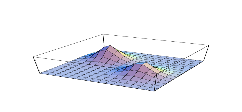
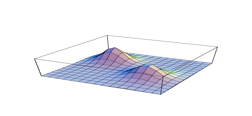
Figure 3: Zero-mode density profiles for the two zero-modes of the lattice caloron (left) on a $4\times 16^{3}$ lattice for $\vec{k}=(1,1,1)$, created with improved cooling ($\varepsilon=0$). The profiles fit well to the two zero-modes for the infinite volume analytic caloron solution (shown on the right at $y\!=\!t\!=\!0$) with $\omega={\scriptstyle{{1\over 4}}}$ and constituents at $\vec{y}_{1}=(2.50,0.12,0.95)$ and $\vec{y}_{2}=(1.38,-0.24,2.67)$, in units where $\beta=l_{t}=1$ (or $a={\scriptstyle{{1\over 4}}}$) and the left most lattice point corresponding to $x=z=0$. The plots give the added densities of the two zero-modes.

Recently also the Weyl-Dirac zero-mode for the infinite volume caloron with non-trivial holonomy was determined analytically [31]. The zero-modes are more localised than the action density and the agreement between the numerically determined zero-mode for the torus caloron is therefore expected to be even better. This is illustrated in Fig. 3, where we compare these exact infinite volume zero-modes with those that are numerically constructed. Since the zero-modes are the ingredients for performing the Nahm transformation, the present comparison shows the numerical accuracy that was achieved. For convenience we have taken for this comparison the parameters that were used in Fig. 1 of Ref. [24], where one can find the action density profiles. In this particular case $\vec{k}=(1,1,1)$ and we duplicate the initial torus in the time-direction, to reach a situation without twist. This gives a charge 2 configuration with two zero-modes, of which one is periodic and the other is anti-periodic. From Ref. [31] one knows that each is localised on one of the constituents. The numerical procedure was to combine the two zero-modes of the doubled lattice in two orthonormal modes, each maximising the overlap with one of the two constituents. Using the large degree of localisation, we have simply added the zero-mode densities together to show the result in one figure, but we stress each lump corresponds to the density of one of the zero-modes. There are no free parameters involved in this comparison and the agreement for the zero-modes is indeed impressive.

In the infinite volume the parameters of the caloron are described by the spatial positions of the two constituents (6 parameters), one overall time position and a $U(1)$ phase rotation that can be undone by a gauge transformation. For large separations of the constituents the caloron becomes static with the two constituent monopoles showing up as separate lumps. On the other extreme when the constituent monopoles are close to each other they fuse into a single lump that looks like an ordinary instanton in $R^{4}$.

Torus instanton configurations ($l_{s}\ll l_{t}$) were studied a few years ago [14, 15]. As $l_{s}/l_{t}\rightarrow 0$ the configurations evolve into well-defined solutions on $T^{3}\times R$. One feature shared by all these torus instanton solutions is that they are local in time. At large times the configurations have to approach a pure gauge, to guarantee the action stays finite. The gauge fields with zero curvature on $T^{3}$ at $t=\pm\infty$ are characterised by their holonomies (spatial Polyakov loops)

$$P_{j}^{\pm}=\lim_{t\rightarrow\pm\infty}{\rm P\,exp}(-i\int_{0}^{l_{j}}A_{j}(t,\vec{x})dx_{j})\quad.$$ (13)

In the presence of a temporal twist $\vec{k}$, the holonomies at both ends are related

$$P_{j}^{+}=e^{2\pi ik_{j}/N}\,P_{j}^{-}\quad.$$ (14)

When we consider $l_{t}/l_{s}$ finite, the instanton has 8 parameters, but the holonomies can not be rigorously defined. In the limit $l_{t}/l_{s}\rightarrow\infty$ they would, however, be related by the twist factors. It is likely that in this limit the three holonomies are part of the moduli that describe the solution (for the infinite volume caloron, gauge zero-modes associated with a variation of $\omega$ are not normalisable and $\omega$ is not a moduli parameter). There are indications that the holonomies fix the scale of the torus instanton [15, 18]. In addition there are of course the four position parameters, and presumably a phase that describes the colour orientation relative to the twist matrices.

The dual gauge field for instantons on $T^{3}\times R$ with temporal twist was shown to be a solution of the abelian Bogomolny equations with point sources [18] that have (due to the self-duality) equal magnetic and electric charges. From this one computes the Maxwell field analytically by summing over the periodic copies of these charges. Essential is that the location of the point charges is determined by the holonomies $P_{j}^{\pm}$. At these specific points on the dual torus the Nahm transformation is modified due to boundary terms in the non-compact directions. This leads to four singularities, whose locations are determined by requiring $\exp(-2\pi il_{j}z_{j})P_{j}^{\pm}$ to have a unit eigenvalue (this leads to a zero-energy state in the Weyl-Dirac Hamiltonian at $t=\pm\infty$ and therefore to non-exponential decay of the zero-mode). The charges are all equal in absolute value, due to Dirac quantisation [18], and opposite in sign for those associated to the holonomies at either end. With temporal twist, the location of the sources with one sign of the charge are displaced by ${\scriptstyle{{1\over 2}}}(\frac{k_{1}}{l_{1}},\frac{k_{2}}{l_{2}},\frac{k_{3}}{l_{3}})$ with respect to the location of the two sources with the opposite sign.

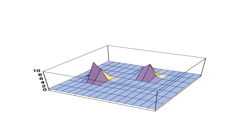
Figure 4: Ratio of the action densities of the Nahm transformed gauge field for a $l_{t}\times 8^{3}$ lattice, dividing the $l_{t}=40$ result by that of $l_{t}=20$. The (approximate) holonomies are given by ${\scriptstyle{{1\over 2}}}{\rm Tr}P_{j}^{-}=-{\scriptstyle{{1\over 2}}}{\rm Tr}P_{j}^{+}=(0.86,0.76,0.082)$.

We illustrate in Fig. 4 how the singularities arise as $l_{t}$ increases. The results are based on a charge 1 instanton on an $20\times 8^{3}$ and $40\times 8^{3}$ lattice with temporal twist $\vec{k}=(1,1,1)$ and holonomies defined by ${\scriptstyle{{1\over 2}}}{\rm Tr}P_{j}^{-}=-{\scriptstyle{{1\over 2}}}{\rm Tr}P_{j}^{+}=(0.86,0.76,0.082)$ (changing $l_{t}$ and making sure the holonomies stay fixed can be achieved by cooling with open boundary conditions, introduced in Ref. [15]). We choose units such that $l_{s}=1$, so that the sources with positive charge are located at $\vec{z}=(0.415,0.387,0.263)$ and $\vec{z}=(0.585,0.613,0.737)$ and the ones with negative charge at $\vec{z}=(0.915,0.887,0.763)$ and $\vec{z}=(0.085,0.113,0.237)$. Fig. 4 is plotted in the plane defined by $z_{3}=0.263$, which is through the position of the first source and still close to the position of the last source. Shown is the ratio of the action density for the $40\times 8^{3}$ lattice over the action density for the $20\times 8^{3}$ lattice.

The nature of the singularities is illuminated by the observation, made before, that the Nahm transformation of the torus instantons are the torus calorons. Thus, the action density peaks correspond to the location of the BPS constituent monopoles. Their mass (associated to $w={\scriptstyle{{1\over 4}}}$) should be given by $8\pi^{2}l_{t}$ (in units where $l_{s}=1$). The result is compatible with the fact that the peak heights of these BPS monopoles scale as $l_{t}^{3}$. Away from the core of these BPS monopoles the field becomes abelian and should become independent of $l_{t}$, as the charge is fixed. Fig. 4 shows that indeed the ratio becomes one outside of the core of the monopoles. The non-abelian core of the BPS monopole shrinks to a point in the limit $l_{t}\rightarrow\infty$, and one is left with the resulting abelian field. This is illustrated in Fig. 5, where we plot the square of the electric field in the plane defined by $z_{3}=0.5$. The numerical result is based on the $40\times 8^{3}$ lattice, for which the plane $z_{3}=0.5$ is far enough away from all sources not to be affected by their non-abelian dressing as $SU(2)$ BPS monopoles of mass $40\pi^{2}$ (in units where $l_{s}=1$). The agreement, that involves no free parameters, is indeed very good.

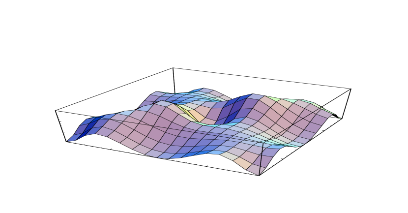
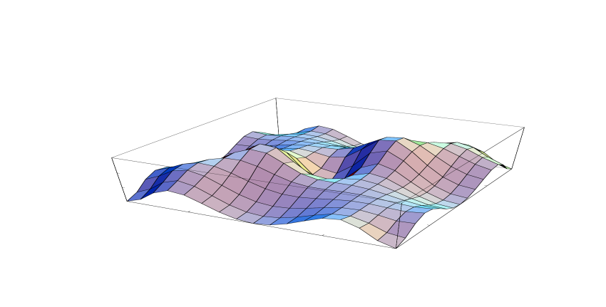
Figure 5: Comparison of $\vec{E}^{2}$ in the plane $z_{3}=0.5$ for the Nahm transformation of the $40\times 8^{3}$ instanton configuration described in the caption of Fig. 4. On the left is the numerical result and on the right the analytic result for $T^{3}\times R$.

The Nahm transformation was constructed by doubling in time, such that at finite $l_{t}$ this corresponds to a charge 2 torus instanton, which is mapped to a charge 2 torus caloron defined on the hypercube $[0,{\scriptstyle{{1\over 2}}}l_{t}^{-1}]\times[0,1]^{3}$. Our general formalism tells us that this is formed by duplicating the Nahm-dual torus, which is half the size. The latter corresponds to a skew lattice, since the twist is not in the Frobenius standard form. The additional lattice generator is precisely the vector ${\scriptstyle{{1\over 2}}}(0,\frac{k_{1}}{l_{1}},\frac{k_{2}}{l_{2}},\frac{k_{3}}{l_{3}})$ giving the displacement of the 2 positive versus the 2 negative sources.

In summary, we have illustrated how the Nahm transformation maps torus instantons into torus calorons, and how the (approximate) holonomies are mapped into the positions of the constituent BPS monopoles. This relation is exact in the limit that $l_{t}\rightarrow\infty$ (resp. 0). To test its validity at finite $l_{t}/l_{s}$ we studied the case with temporal twist $\vec{k}=(0,1,0)$ ($\vec{m}=(0,0,0)$). One cannot have both the original and Nahm-dual torus to be spatially symmetric, due to the asymmetric twist, but that is not important for the general conclusion about the mapping we are studying. If our original torus has size $l_{t}\times l_{s}^{3}$, $\hat{\Lambda}=\tilde{\Lambda}_{0}$ has size $\frac{1}{2l_{t}}\times\frac{1}{l_{s}}\times\frac{1}{2l_{s}}\times\frac{1}{l_{s}}$. The twist vectors for the Nahm transform are the same as the original ones.

By means of improved cooling ($\varepsilon=0$) we have generated a lattice torus caloron configuration [24]. The relative distance between the two constituent monopoles can be tuned by using different values of the parameter $\varepsilon$ [24]. On the other hand, it is possible to use a modified version of cooling [15] (fixing the field to have zero colour magnetic fields at $t=0$ and $t=l_{t}$ in terms of prescribed holonomies) in order to produce torus instanton configurations with fixed holonomies. If we choose these to be the ones determined by the location of the monopole constituents of the torus caloron, then the numerical Nahm transformation [25] can be applied to each of these configurations and has to give back the other configuration, up to a translation. This is illustrated in Fig. 6. The somewhat larger numerical differences are in part due to the not sufficiently large ratio for $l_{t}/l_{s}$ which, for the required values of the holonomies, enforces a rather narrow instanton which is not easily stabilised on the lattice. Results for a smaller value of $l_{t}/l_{s}$ (not shown) confirm this improvement with increasing $l_{t}/l_{s}$. Going to even a larger ratio is however computationally too expensive. The comparison confirms that the holonomies of the time-twisted torus instanton are part of the moduli.

Figure 6: Comparison between the action densities of a numerical $Q=1$ instanton with twist $\vec{k}=(0,1,0)$ and $\vec{m}=\vec{0}$, living on a $32\times 8\times 4\times 8$ lattice, and the Nahm transformation of $Q=1$ torus caloron with the same twist, living on a $4\times 32^{3}$ lattice. The constituent locations were used to fix the holonomies in generating the torus instanton. Depicted values correspond to points in the $4\times 32^{3}$ lattice, along the $x$ direction. The continuum units are such that $l_{t}=1$ for the caloron.

3.3 Spatial twist $Q=1$

We will conclude by discussing the case of spatial twist ($\vec{k}=\vec{0}$), for which we take $\vec{m}=(0,1,0)$. If our original torus has size $l_{t}\times l_{s}^{3}$, the Nahm dual torus for this twist has size $\frac{1}{l_{t}}\times\frac{1}{2l_{s}}\times\frac{1}{l_{s}}\times\frac{1}{2l_{s}}$ (to obtain instead a spatially symmetric dual torus we should apply the Nahm transformation to a torus with size $l_{t}\times{\scriptstyle{{1\over 2}}}l_{s}\times l_{s}\times{\scriptstyle{{1\over 2}}}l_{s}$). As before, the dual gauge field has the same spatial twist as the original gauge field. The phenomenology of these configurations, for the large aspect ratios we are interested in, is different to the previous case with temporal twist. But there are also quite interesting analogies that may be important for the case $l_{t}=l_{s}$, where from the Euclidean point of view there should be no essential difference between twist in space or time.

The analysis of Ref. [24] shows that for $l_{s}/l_{t}$ large, torus calorons with spatial twist are given by configurations that approximate the infinite volume caloron with arbitrary holonomy, parametrised by $\omega\in[0,{\scriptstyle{{1\over 2}}}]$, such that the two constituent monopoles have in general differing masses, $16\pi^{2}\omega/l_{t}$ and $8\pi^{2}(1-2\omega)/l_{t}$. But now their relative positions are fixed and determined by the spatial twist. This contrasts with the situation for temporal twists for which the value of $w$ is fixed, but the relative position is arbitrary.

Torus instantons with twisted boundary conditions in space, and $l_{s}/l_{t}$ small, have been studied extensively in relation to the Hamiltonian formulation in a twisted box [21]. The outcome of these studies [22] showed that the configurations can be described in terms of two $Q={\scriptstyle{{1\over 2}}}$ twisted instantons ($2Q$ twisted instantons in the case of higher charges), that have both twist in space and time. The net twist in time, however, vanishes. We can view the $Q={\scriptstyle{{1\over 2}}}$ constituents of the $Q=1$ instanton in very much the same way as the monopole constituents for the caloron. It was found that the space-time locations of these twisted instanton lumps can be arbitrary. Only when they are very close to each other, they merge into a single lump. In that region, when the size of the lump becomes small compared to $l_{s}$, the configuration behaves like the ordinary instanton in $R^{4}$. There are two very simple specific examples where this constituent nature of the torus instantons with spatial twist is apparent. Take a $Q={\scriptstyle{{1\over 2}}}$ instanton with twist $\vec{m}=\vec{k}=(0,1,0)$ and duplicate either in the 0 or 2 direction to remove the time twist. The result is a $Q=1$ instanton with spatial twist. Either the two lumps have the same spatial positions and are separated maximally along the time direction, or they have equal time positions and are maximally separated along the space direction.

We now turn our attention to studying how the Nahm transformation relates these torus instantons and calorons. For the above example built from two $Q={\scriptstyle{{1\over 2}}}$ instantons, this can directly be understood in terms of the results of section 3.1, where it was shown that the dual of such a $Q={\scriptstyle{{1\over 2}}}$ instanton is a BPS monopole, with twist $\vec{k}=\vec{m}=(0,1,0)$. Duplication of the instanton in the 0 direction is dual to duplication of the BPS monopole in the 2 direction, and we do get a caloron with maximal separation of the ($\omega={\scriptstyle{{1\over 4}}}$) constituents in the direction of the spatial twist. On the other hand, duplication of the instanton in the 2 direction is dual to duplication of the BPS monopole in the 0 direction. This doubles the mass of the constituent monopole and corresponds to a caloron with trivial holonomy $\omega=0$ or ${\scriptstyle{{1\over 2}}}$ (the other constituent is massless and therefore absent). This establishes that, with twist in space, $\omega$ need not be ${\scriptstyle{{1\over 4}}}$.

To deal with a more general case, we consider the $Q=1$ instanton with spatial twist being made out of two $Q={\scriptstyle{{1\over 2}}}$ ($\vec{m}=(0,1,0)$, $\vec{k}$ arbitrary such that $\vec{k}\cdot\vec{m}=1({\rm mod}\,2$)) with an arbitrary time separation, i.e. no longer obtained by duplication in the time direction. To study some of the properties of its Nahm transform, we consider the limit $l_{s}\rightarrow 0$. In this limit all spatial dependence is removed and the two $Q={\scriptstyle{{1\over 2}}}$ instantons shrink to two points, specified by their positions in time. In one dimension curvature can be non-trivial only at point-like singularities, so the curvature vanishes everywhere, except at the locations of the $Q={\scriptstyle{{1\over 2}}}$ instantons, where the field strength becomes singular. The curvature free regions are described by a constant abelian gauge field $\hat{A}_{j}$, making a jump at the positions of the $Q={\scriptstyle{{1\over 2}}}$ instantons. In this limit, for a single $Q={\scriptstyle{{1\over 2}}}$ instanton, the twist determines the jump in the constant gauge field to be $\Delta\hat{A}_{j}=\pi k_{j}/l_{s}$ (relevant for the case of space twist, so as to assure that Eq. (14) is satisfied. In the general case, where the values of the Polyakov loops are not fixed (see below), there is more freedom). The $Q=1$ instanton is therefore described by

$$\hat{A}_{j}=2\pi(\xi_{j}+{\scriptstyle{{1\over 2}}}k_{j}\chi_{[t_{a},t_{b}]}(t)/l_{s})\quad,$$ (15)

where $\xi_{j}$ (and $\hat{A}_{0}$) are arbitrary constants (fixed for spatial twist, see later) and $\chi_{[t_{a},t_{b}]}(t)$ is the characteristic function of the interval $t\in[t_{a},t_{b}]$. This result agrees exactly with the Nahm transformed gauge field of the infinite volume caloron [16]. We can identify ${\scriptstyle{{1\over 2}}}\vec{k}/l_{s}(=\hat{a}\pi\rho^{2})$ with the distance vector between the two constituents (in units set by $l_{t}=1$) and $\omega={\scriptstyle{{1\over 2}}}(t_{b}-t_{a})$ with its holonomy (see the second of Ref. [16], Eqs. (41) and (65), for the precise definitions of $\rho$ and $\hat{a}$).

Figure 7: Comparison between the action densities of the numerical Nahm transform of a torus instanton and the appropriate infinite volume analytic caloron solution. The original field lives on a $80\times 4\times 8\times 4$ lattice with twist $\vec{k}=(0,0,0)$, $\vec{m}=(0,1,0)$. Units are set by $l_{t}=1$. The temporal distance between the two $Q={\scriptstyle{{1\over 2}}}$ constituents for the instanton corresponds to a caloron with $\omega=d_{0}/2=0.311$. The plot is along the line connecting the centers of the two constituent monopoles, defined by $z_{1}=z_{3}=5$ as determined by the spatial holonomies of the instanton.

It may seem that for the Nahm gauge field of the caloron $t_{a}=-\omega$ and $t_{b}=\omega$ are fixed, but one should of course realise that $\hat{A}$ is still self-dual, away from the singularities, when $t$ is shifted over a constant. We conclude that the holonomy of the caloron fixes the relative locations of the $Q={\scriptstyle{{1\over 2}}}$ instanton lumps under the Nahm transformation, whereas the holonomies of the instanton, determined in each of the two flat regions (for $l_{s}\rightarrow 0$), fix the relative locations of the constituent monopoles of the caloron. Their difference vector ${\scriptstyle{{1\over 2}}}\vec{m}/l_{s}$, remarkably, agrees with maximal separation on the dual torus along the direction determined by the spatial twist. This derivation is as rigorous, in the limit $l_{s}\rightarrow 0$, as the one for $T^{3}\times[0,l_{t}]$, in the limit $l_{t}\rightarrow\infty$ and has given a beautifully consistent picture of the dual relationship between the moduli spaces of the calorons and finite volume instantons.

To test this picture at finite $l_{s}$ we have made use of our numerical methods. We started with a configuration on an $80\times 4\times 8\times 4$ lattice containing two $Q={\scriptstyle{{1\over 2}}}$ torus twisted instantons (with $\vec{m}=\vec{k}=(0,1,0)$) separated in time by a distance $d_{0}$. In units where $l_{t}=1$ (so $l_{s}=1/10$), the lattice $\Lambda$ is generated by $e_{0}=(1,0,0,0)$, $e_{1}=(0,l_{s}/2,0,0)$, $e_{2}=(0,0,l_{s},0)$ and $e_{3}=(0,0,0,l_{s}/2)$. The dual torus $R^{4}/\tilde{\Lambda}_{0}$ has as unit cell $[0,1]\times[0,l_{s}^{-1}]^{3}$. This configuration is constructed in several steps. First one starts with a $Q={\scriptstyle{{1\over 2}}}$ configuration on a $40\times 4\times 8\times 4$ lattice with twist $\vec{k}=\vec{m}=(0,1,0)$. Using a time reversal and parity transformation one obtains a second $Q={\scriptstyle{{1\over 2}}}$ instanton with the Polyakov loops at $t\approx\pm\infty$ interchanged. One can glue the two configurations together at arbitrary time separation $d_{0}$ and transform them appropriately to trivial twist matrices in time. If $d_{0}\gg l_{s}$ this procedure gives an approximate self-dual solution on the required torus and with spatial twist. The small deviations from self-duality induced by the procedure can be eliminated by cooling with $\varepsilon=0$. We end up with a $Q=1$ configuration with the desired properties.

Figure 8: The same as in Fig. 7, but for a temporal distance corresponding to $d_{0}=0.786$.

A few remarks are in order, concerning the values of the Polyakov loops for the space twisted instantons. Eqs. (12) and (13) are only valid in the gauge where the appropriate $\Omega_{a}(x)$ are trivial. Such a gauge was assumed for the discussion in sect. 3.2. The general formula for a Wilson loop that closes by the shift over a period reads [32]

$$P_{\mu}(x)={\rm P\,exp}(-i\int^{l_{\mu}}_{0}A_{\mu}(x)dx_{\mu})\,\Omega_{e^{(\mu)}}(x)\quad.$$ (16)

In the presence of a space twist the $P_{i}$ are not arbitrary, but uniquely determined (up to some discrete transformations) by the twist. This can be seen as follows. Since the configuration is exponentially localised in time, it goes to a pure gauge at $\pm\infty$. Now one can choose a gauge in which $A_{i}(t=\infty)=0$, fixing $\xi_{i}=0$ in Eq. (15), for which the twist matrices $\Omega_{e^{(i)}}$ are constant and the holonomy is given precisely by these matrices. The fact that $\Omega_{e^{(1)}}$ and $\Omega_{e^{(3)}}$ anticommute (as a result of the twist), implies they can be brought to the form $i\sigma_{1}$ and $i\sigma_{3}$, respectively. On the other hand, the constant twist matrix for the $2$ direction has to commute with these Pauli matrices and therefore must be $\pm I$. This fixes the Polyakov loops for the $Q=1$ space twisted instanton at both $t=\infty$ and $t=-\infty$ to be ${\scriptstyle{{1\over 2}}}{\rm Tr}P_{1}={\scriptstyle{{1\over 2}}}{\rm Tr}P_{3}=0$ and ${\scriptstyle{{1\over 2}}}{\rm Tr}P_{2}=\pm 1$, depending on whether we choose the twist matrix in direction 2 to be $\pm I$. The location of the caloron constituents are determined by the holonomies to be at $\vec{z}=(5,0,5)$, and the one displaced by ${\scriptstyle{{1\over 2}}}\vec{m}/l_{s}$ from it, i.e. $\vec{z}=(5,5,5)$.

We have generated two such configurations with time separations between the $Q={\scriptstyle{{1\over 2}}}$ instanton constituents given by $d_{0}=0.622$ and $d_{0}=0.786$. In Figs. 7 and 8 we compare the Nahm transformed results with the infinite volume analytic caloron solutions and the holonomy fixed to $\omega=d_{0}/2$. Plotted is the action density along the line joining the two monopoles. The comparison is very good taking into account that there are no free parameters. The mismatch at the peaks can be attributed to the fact that the data points correspond to a finite ratio $\l_{t}/l_{s}=1/10$, which is zero for the analytic result. A direct comparison with numerical data at this fixed ratio is difficult due to its small value, and seems unnecessary given the agreement shown in Figs. 7-8.

4 Conclusions

By now our knowledge of self-dual configurations on the torus has come from various sources. Apart from general existence proofs and consequences of the index theorem, information in this field has arisen from both numerical studies based on lattice gauge theories and analytical results obtained on manifolds having compact and non-compact directions. Most of the interest and information refers to self-dual configurations on spatially symmetric tori of size $l_{t}\times l_{s}^{3}$ for large and small aspect ratios, known as torus instantons ($l_{s}/l_{t}\ll 1$) and torus calorons ($l_{s}/l_{t}\gg 1$). In this paper we have studied the Nahm transformation that relates $SU(N)$ self-dual gauge fields of charge $Q$ with twisted boundary conditions on a torus, to $SU(N_{0}Q)$ self-dual gauge fields of charge $N/N_{0}$ on the dual torus. Here $N_{0}$ is determined by the twist. We found that torus calorons and instantons are dual to each other. This provides information on their respective moduli spaces, which is fully consistent with the structure suggested by numerical studies. In particular, it allows us to understand the findings of Ref. [24]. The most notable result is the duality observed between holonomies and the location of constituent structures (BPS monopoles or twisted instantons), as suggested by analysis of the Nahm transformation of configurations living in $T^{3}\times R$ and $R^{3}\times S^{1}$. We showed how the abelian Nahm connections with singularities obtained in this case, result from the collapse of the non-abelian core of the constituents into point-like singularities, which act as sources of the surviving abelian field. Thus, all the information fits nicely into a unified picture.

Our results might be of help in different respects. Recently the ($T$) dualities discussed here have played important roles in D-brane and string compactifications and our findings concerning the relation between holonomies and constituent positions is an interesting one also in this context. For the low charges studied here we saw that the basic constituent is a twisted instanton, with charge $Q={\scriptstyle{{1\over 2}}}$ in $SU(2)$, which shows up as a BPS monopole at finite temperature. We have shown that this fractional instanton maps onto itself under the Nahm duality transformation, a property guaranteed by the fact that for $SU(2)$ the twist is preserved under the duality transformation and the only freedom is the position of these twisted instantons. It would be interesting to see in which sense these constituents do continue to play an important role at higher charges. Finally, we hope that the work presented here will lead to a more complete analytic understanding.

Appendix

In this appendix we will provide the proofs of the basic ingredients of the flavour construction of Nahm’s transformation for non-trivial twisted boundary conditions ($\vec{k}$, $\vec{m}\neq\vec{0})$. In particular, we will present in a basis independent way the derivation of the characterisation for the Nahm-dual torus and its corresponding dual twist. This complements the results of Ref. [26].

Our starting point is the set of Weyl zero-modes $\Psi_{z}^{i\alpha}(x)$ satisfying the boundary conditions of Eq. (9). Consider now the behaviour of these zero-modes under translation of the variables $z$. It is easy to see that given a solution $\Psi_{z}(x)$ of the Weyl equation one can construct a new solution of the Weyl equation as follows:

$$\chi^{(y)}_{z}(x)\equiv e^{-2\pi iy(x)}\,\Psi_{z+y}(x)\quad,$$ (17)

for any element $y\in\tilde{R}^{4}$ (as usual the space of linear forms $\tilde{R}^{4}$ can be identified with $R^{4}$, and $y(x)\equiv y\cdot x$). Applying this to an orthonormal set of solutions of the Weyl equation one obtains a new set. This set satisfies different boundary conditions, obtained from Eq. (9) by replacing the twist eating matrices $\Gamma(a)$,

$$\Gamma(a)\longrightarrow\Gamma^{\prime}(a)=e^{2\pi iy(a)}\,\Gamma(a)\quad.$$ (18)

We thus see that there is a correspondence between translations in $z$ and different choices of twist-eating solutions.

In general the matrices $\Gamma^{\prime}(a)$ constitute an inequivalent set of solutions to the original $\Gamma(a)$. However, for special values of $y$ the two sets are unitarily equivalent (related by a similarity transformation). For those values of $y$, denoted by $\hat{a}$, there exist $U(N_{0})$ matrices $\tilde{\Gamma}(\hat{a})$ satisfying

$$\tilde{\Gamma}(\hat{a})\,\Gamma(a)=e^{2\pi i\hat{a}(a)}\,\Gamma(a)\,\tilde{\Gamma}(\hat{a})\quad.$$ (19)

This formula shows a nice duality between both sets of $U(N_{0})$ matrices. Before investigating for which $\hat{a}$ these equations have solutions, we want to discuss its consequences. For all values $\hat{a}$, for which Eq. (19) has solutions, we can construct the functions

$$e^{-2\pi i\hat{a}(a)}\,\Psi_{z+\hat{a}}^{j\alpha}(x)\,\tilde{\Gamma}^{ji}(\hat{a})$$ (20)

which form a new orthonormal set of solutions of the Weyl equation with the same boundary conditions Eq. (9). Thus, they can be expressed as a unitary combination of the original set of zero-modes. We arrive at the main formula:

$$\Psi_{z+\hat{a}}^{i\alpha}(x)=e^{2\pi i\hat{a}(a)}\,\tilde{\Gamma}^{*}_{ij}(\hat{a})\,\Psi_{z}^{j\beta}(x)(\hat{\Omega}_{\hat{a}}^{\dagger}(z))^{\beta\alpha}\quad.$$ (21)

From this one can deduce that for all $\hat{a}$ the Nahm transformed gauge field satisfies

$$\hat{A}_{\mu}(z+\hat{a})=[\hat{\Omega}_{\hat{a}}(z)]\,\hat{A}_{\mu}(z)$$ (22)

One easily sees that the set of $\hat{a}$ define a lattice $\hat{\Lambda}$, which we will call the Nahm-dual lattice. It is a sublattice of $\tilde{\Lambda}$, the lattice dual to $\Lambda$. We define the Nahm transformation of the original self-dual gauge field with twist as the restriction of $\hat{A}$ to the Nahm-dual torus $R^{4}/\hat{\Lambda}$. This is a $U(N_{0}Q)$ self-dual gauge field with topological charge $\hat{Q}=N_{0}N/|\tilde{\Lambda}/\hat{\Lambda}|$, where $|\tilde{\Lambda}/\hat{\Lambda}|$ stands for the number of unit cells of $\hat{\Lambda}$ that fit in a unit cell of $\tilde{\Lambda}$, or the number of elements in $\hat{\Lambda}$(mod $\tilde{\Lambda}$). The matrices $\hat{\Omega}_{\hat{a}}(z)$ are the corresponding twist matrices.

Now let us investigate the solutions to Eq. (19) and the characterisation of $\hat{\Lambda}$. For that it is essential to use some properties of the twist eating solutions. One can prove [1] that the set of matrices $\Gamma(a)$ contains a set of $N_{0}^{2}$ linearly independent matrices, which form a basis of the space of all $N_{0}\times N_{0}$ matrices. Actually, to construct this basis one has to select a representative of the quotient lattice $\Lambda/\Lambda_{0}$. Its order is precisely $N_{0}^{2}$. The sublattice $\Lambda_{0}$ can also be defined as the one associated to the matrices $\Gamma(a)$ commuting with all other $\Gamma(a^{\prime})$ for any $a^{\prime}\in\Lambda$. We call it the center lattice. Using this fact one can, after some effort, prove that indeed the matrices $\tilde{\Gamma}(\hat{a})$ do coincide, up to a phase factor, with the original matrices $\Gamma(a)$. In more mathematical terms, we can say that there exists a mapping $\phi$ from $\hat{\Lambda}$ to $\Lambda$ such that

$$\tilde{\Gamma}(\hat{a})=e^{i\varphi(\hat{a})}\,\Gamma(\phi(\hat{a}))\quad.$$ (23)

where $\varphi(\hat{a})$ is an arbitrary phase. From this we can identify $\hat{\Lambda}$. Let $a$ be an element of $\Lambda_{0}$, then it commutes with all matrices $\Gamma(a^{\prime})$ for any $a\in\Lambda^{\prime}$, this includes the matrices $\tilde{\Gamma}(\hat{a})$. Inspecting Eq. (19) we conclude that $\hat{a}(a)\in Z$ for any $a\in\Lambda_{0}$. Therefore $\hat{\Lambda}=\tilde{\Lambda}_{0}$, the Nahm dual lattice coincides with the dual lattice of the center lattice. One can also see that the center lattice of $\hat{\Lambda}$ coincides with $\tilde{\Lambda}$. From here it is immediate to see that the Nahm-dual of the Nahm-dual gives back the original lattice.

There is one extra ingredient which has to be worked out, namely what is the Nahm dual twist. This follows from Eq. (23) and Eq. (8). We have

$$\tilde{\Gamma}(\hat{a})\,\tilde{\Gamma}(\hat{a}^{\prime})=e^{-2\pi i\hat{\cal N}(\hat{a},\hat{a}^{\prime}))}\,\tilde{\Gamma}(\hat{a}^{\prime})\,\tilde{\Gamma}(\hat{a})$$ (24)

with

$$\hat{\cal N}(\hat{a},\hat{a}^{\prime})=-{\cal N}(\phi(\hat{a}),\phi(\hat{a}^{\prime}))\quad.$$ (25)

Eq. (21) is only consistent provided the Nahm-dual twist matrices $\hat{\Omega}_{\hat{a}}(z)$ satisfy twisted boundary conditions analogous to Eq. (2) with the skew symmetric form ${\cal N}$ replaced by $\hat{\cal N}$, the dual twist form.

References

- [1] A. González-Arroyo, Yang-Mills fields on the four-dimensional torus. Part 1.: Classical theory, hep-th/9807108, in: Advanced School for Nonperturbative Quantum Field Physics, eds. M. Asorey and A. Dobado, World Scientific 1998, 57.
- [2] G. ‘t Hooft, Nucl. Phys. B153 (1979) 141; Acta Physica Aust. Suppl. XXII (1980) 531.
- [3] M. García Pérez, A. González-Arroyo and B. Söderberg, Phys. Lett. B235 (1990) 117.
- [4] M. García Pérez and A. González-Arroyo, Jour. Phys. A26 (1993) 2667.
- [5] P. Braam, A. Maciocia and A. Todorov, Inv. Math. 108 (1992) 419.
- [6] P. Braam and P. van Baal, Comm. Math. Phys. 122 (1989) 267.
- [7] C.H. Taubes, J. Diff. Geom. 19 (1984) 517.
- [8] M.F. Atiyah, N.J. Hitchin, V.G. Drinfeld, Yu. I. Manin, Phys. Lett. 65 A (1978) 185.
- [9] W. Nahm, Phys. Lett. 90B (1980) 413; Self-dual monopoles and calorons, in: Lect. Notes in Physics. 201, eds. G. Denardo, e.a. (1984) p.189.
- [10] G. ‘t Hooft, Comm. Math. Phys. 81 (1981) 267; P. van Baal Comm. Math. Phys. 94 (1984) 397.
- [11] P. van Baal, Nucl. Phys. B(Proc.Suppl.)49 (1996) 238 (hep-th/9512223).
- [12] B.J. Harrington and H.K. Shepard, Phys. Rev. D17 (1978) 2122; D18 (1978) 2990.
- [13] D.J. Gross, R.D. Pisarski and L.G. Yaffe, Rev. Mod. Phys. 53 (1983) 43.
- [14] M. García Pérez, A. González-Arroyo, J. Snippe and P. van Baal, Nucl. Phys. B413 (1994) 535 (hep-lat/9309009).
- [15] M. García Pérez, A. González-Arroyo, J. Snippe and P. van Baal, Nucl. Phys. B(Proc.Suppl)34 (1994) 222 (hep-lat/9311032).
- [16] T.C. Kraan and P. van Baal, Phys. Lett. B428 (1998) 268 (hep-th/9802049); Nucl. Phys. B533 (1998) 627 (hep-th/9805168); Phys. Lett. B435 (1998) 389 (hep-th/9806034).
- [17] K. Lee and P. Yi, Phys. Rev. D56 (1997) 3711 (hep-th/9702107); K. Lee, Phys. Lett. B426 (1998) 323 (hep-th/9802012); K. Lee and C. Lu, Phys. Rev. D58 (1998) 025011 (hep-th/9802108).
- [18] P. van Baal, Phys. Lett. B448 (1999) 26 (hep-th/9811112).
- [19] J. Snippe, Phys. Lett. B335 (1994) 395-402 (hep-th/9405129).
- [20] M. García Pérez, A. González-Arroyo, A. Montero and C. Pena, Nucl. Phys. B(Proc.Suppl.)63 (1998) 501 (hep-lat/9709107).
- [21] M. García Pérez, A. González-Arroyo, P. Martínez, et al (RTN Collaboration) Phys. Lett. B305 (1993) 366 (hep-lat/9302007).
- [22] A. González-Arroyo, P. Martínez and A. Montero, Phys. Lett. B359 (1995) 159 (hep-lat/9507006).
- [23] A. González-Arroyo and A. Montero, Phys. Lett. B442 (1998) 273 (hep-th/9809037).
- [24] M. García Pérez, A. González-Arroyo, A. Montero and P. van Baal, Calorons on the lattice - a new perspective, hep-lat/9903022.
- [25] A. González-Arroyo and C. Pena, JHEP 09 (1998) 013.
- [26] A. González-Arroyo, On Nahm’s transformation with twisted boundary conditions, hep-th/9811041.
- [27] E. Cohen and C. Gómez, Nucl. Phys. B223 (1983) 183.
- [28] M.F. Atiyah, I.M. Singer, Ann. Math. 93 (1971) 119.
- [29] P. van Baal, Comm. Math. Phys. 85 (1982) 529.
- [30] J. Groeneveld, J. Jurkiewicz and C.P. Korthals Altes, Physica Scripta 23 (1981) 1022.
- [31] M. García Pérez, A. González-Arroyo, C. Pena and P. van Baal, Weyl-Dirac zero-mode for calorons, hep-lat/9905016, Phys. Rev. D, Rapid Comm., to appear.
- [32] P. van Baal, Twisted Boundary Conditions: A Non-Perturbative Probe for Pure Non-Abelian Gauge Theories, PhD-Thesis, Utrecht, July 1984.
- [33] P. van Baal and B. van Geemen, J. Math. Phys. 27 (1986) 455; Proc. K. Ned. Akad. Wet. B89 (1986) 39; D.R. Lebedev and M.I. Polikarpov, Nucl. Phys. B269 (1986) 285.