hep-th/9905134

May 1999

$Osp(N|4)$ supermultiplets

as conformal superfields on $\partial AdS_{4}$ and

the generic form of $N=2,\,d=3$ gauge theories ${}^{*}{}^{\dagger}$
Davide Fabbri, Pietro Fré, Leonardo Gualtieri and Piet Termonia

Dipartimento di Fisica Teorica, Universitá di Torino, via P. Giuria 1, I-10125 Torino,

Istituto Nazionale di Fisica Nucleare (INFN) - Sezione di Torino, Italy

In this paper we fill a necessary gap in order to realize the explicit comparison between the Kaluza Klein spectra of supergravity compactified on $AdS_{4}\times X^{7}$ and superconformal field theories living on the world volume of M2–branes. On the algebraic side we consider the superalgebra $Osp({\cal N}|4)$ and we study the double intepretation of its unitary irreducible representations either as supermultiplets of particle states in the bulk or as conformal superfield on the boundary. On the lagrangian field theory side we construct, using rheonomy rather than superfield techniques, the generic form of an ${\cal N}=2,d=3$ gauge theory. Indeed the superconformal multiplets are supposed to be composite operators in a suitable gauge theory.

 ^∗ Supported in part by EEC under TMR contract ERBFMRX-CT96-0045

1 Introduction

One of the most exciting developments in the recent history of string theory has been the discovery of the holographic AdS/CFT correspondence [1, 2, 3, 4, 5, 6]:

$$\mbox{SCFT on $\partial(AdS_{p+2})$}\quad\leftrightarrow\quad\mbox{SUGRA on $AdS_{p+2}$}$$ (1.1)

between a $d=p+1$ quantum superconformal field theory on the boundary of anti de Sitter space and classical Kaluza Klein supergravity [7, 8, 9, 10, 11], [12, 13, 14, 15, 16, 17], [18, 19, 20], [21, 22, 23, 24, 25, 26] emerging from compactification of either superstrings or M-theory on the product space

$$AdS_{p+2}\,\times\,X^{D-p-2}\,,$$ (1.2)

where $X^{D-p-2}$ is a $D-p-2$–dimensional compact Einstein manifold.

The present paper deals with the case:

$$p=2\quad\leftrightarrow\quad d=3$$ (1.3)

and studies two issues:

1. The relation between the description of unitary irreducible representations of the $Osp(2|4)$ superalgebra seen as off–shell conformal superfields in $d=3$ or as on–shell particle supermultiplets in $d=4$ anti de Sitter space. Such double interpretation of the same abstract representations is the algebraic core of the AdS/CFT correspondence.

2. The generic component form of an ${\cal N}=2$ gauge theory in three space-time dimensions containing the supermultiplet of an arbitrary gauge group, an arbitrary number of scalar multiplets in arbitrary representations of the gauge group and with generic superpotential interactions. This is also an essential item in the discussion of the AdS/CFT correspondence since the superconformal field theory on the boundary is to be identified with a superconformal infrared fixed point of a non abelian gauge theory of such a type.

Before presenting our results we put them into perspective through the following introductory remarks.

1.1 The conceptual environment and our goals

The logical path connecting the two partners in the above correspondence (1.1) starts from considering a special instance of classical $p$–brane solution of $D$–dimensional supergravity characterized by the absence of a dilaton ($a=0$ in standard $p$–brane notations) and by the following relation:

$$\frac{d{\widetilde{d}}}{D-2}=2$$ (1.4)

between the dimension $d\equiv p+1$ of the $p$–brane world volume and that of its magnetic dual ${\widetilde{d}}\equiv D-p-3$. Such a solution is given by the following metric and $p+2$ field strength:

$$ds^{2}_{brane} = \left(1+\frac{k}{r^{\widetilde{d}}}\right)^{-\frac{{\widetilde{d}}}{(D-2)}}\,dx^{m}\otimes dx^{n}\,\eta_{mn}-\left(1+\frac{k}{r^{\widetilde{d}}}\right)^{\frac{{d}}{(D-2)}}\,\left(dr^{2}+r^{2}\,ds^{2}_{X}(y)\right)\,,$$

$$F\equiv dA = \lambda(-)^{p+1}\epsilon_{m_{1}\dots m_{p+1}}dx^{m_{1}}\wedge\dots\wedge dx^{m_{p+1}}\wedge\,dr\,\left(1+\frac{k}{r^{\widetilde{d}}}\right)^{-2}\,\frac{1}{r^{{\widetilde{d}}+1}}\,.$$ (1.5)

In eq. (1.5) $ds^{2}_{X}(y)$ denotes the Einstein metric on the compact manifold $X^{D-p-2}$ and the $D$ coordinates have been subdivided into the following subsets

• $x^{m}$ $(m=0,\dots,p)$ are the coordinates on the $p$–brane world–volume,

• $r=\mbox{radial}$ $\oplus$ $y^{x}=\mbox{angular on $X^{D-p-2}$}$ $(x=D-d+2,\dots,D)$ are the coordinates transverse to the brane.

In the limit $r\to 0$ the classical brane metric $ds^{2}_{brane}$ approaches the following metric:

$$\begin{array}[]{ccccc}ds^{2}&=&\underbrace{\frac{r^{2{\widetilde{d}}/d}}{k^{2/d}}\,dx^{m}\otimes dx^{n}\,\eta_{mn}-\frac{k^{2/{\widetilde{d}}}}{r^{2}}\,dr^{2}}&-&\underbrace{\phantom{\frac{1}{1^{1}}}k^{2/{\widetilde{d}}}\,ds^{2}_{X}(y)\phantom{\frac{1}{1^{1}}}}\\ \hbox{}\hfil&\hbox{}\hfil&AdS_{p+2}&\times&X^{D-p-2}\,,\\ \end{array}$$ (1.6)

that is easily identified as the standard metric on the product space $AdS_{p+2}\times X^{D-p-2}$. Indeed it suffices to set:

$$\rho=r^{{\widetilde{d}}/d}\,k^{2(d+{\widetilde{d}})/d^{2}}$$ (1.7)

to obtain :

$$ds^{2}_{brane} \stackrel{{\scriptstyle r\to 0}}{{\approx}} k^{2/{\widetilde{d}}}\,\left(ds^{2}_{AdS}-ds^{2}_{X}(y)\right)\,,$$ (1.8)

$$ds^{2}_{AdS} = \left(\rho^{2}\,dx^{m}\otimes dx^{n}\,\eta_{mn}-\frac{d\rho^{2}}{\rho^{2}}\right)\,,$$ (1.9)

where (1.9) is the canonical form of the anti de Sitter metric in solvable coordinates [49].

On the other hand, for $r\to\infty$ the brane metric approaches the limit:

$$\begin{array}[]{ccccc}ds^{2}_{brane}&\stackrel{{\scriptstyle r\to\infty}}{{\approx}}&\underbrace{dx^{m}\otimes dx^{n}\,\eta_{mn}}&-&\underbrace{dr^{2}+r^{2}\,ds^{2}_{X}(y)}\\ \hbox{}\hfil&\hbox{}\hfil&M_{p+1}&\hbox{}\hfil&C\left(X^{D-p-2}\right)\,,\end{array}$$ (1.10)

where $M_{p+1}$ denotes Minkowski space in $p+1$ dimensions while $C\left(X^{D-p-2}\right)$ denotes the $D-p-1$ dimensional metric cone over the horizon manifold $X^{D-p-2}$. The key point is that (compactified) Minkowski space can also be identified with the boundary of anti de Sitter space:

$$\partial\left(AdS_{p+2}\right)\equiv M_{p+1}\,,$$ (1.11)

so that we can relate supergravity on $AdS_{p+2}\times X^{D-p-2}$ to the gauge theory of a stack of $p$–branes placed in such a way as to have the metric cone as transverse space (see fig.1)

$$C\left(X^{D-p-2}\right)=\mbox{transverse directions to the branes.}$$ (1.12)

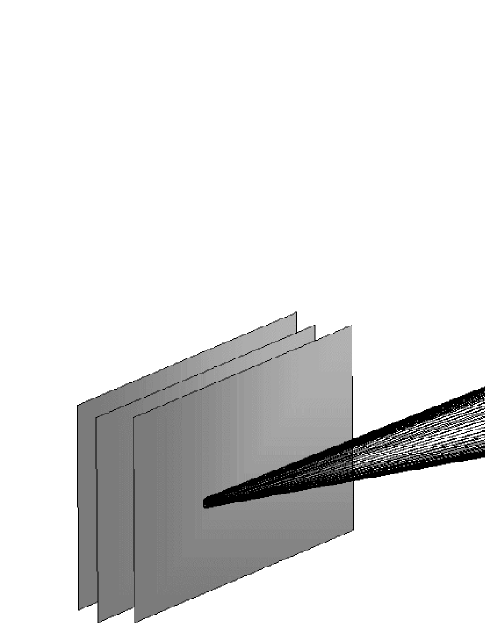
Figure 1: The metric cone $C\left(X^{D-p-2}\right)$ is transverse to the stack of branes

According to current lore on brane dynamics [50, 51, 52, 53], if the metric cone $C(X^{D-p-2})$ can be reintepreted as some suitable resolution of an orbifold singularity [54, 55, 56, 57]:

$$C(X^{D-p-2}) = \mbox{resolution of }\,\frac{R^{D-p-1}}{\Gamma}\,,$$

$$\Gamma = \mbox{discrete group},$$ (1.13)

then there are means to identify a gauge theory in $M_{p+1}$ Minkowski space with supersymmetry ${\cal N}$ determined by the holonomy of the metric cone, whose structure and field content in the ultraviolet limit is determined by the orbifold ${R^{D-p-1}}/{\Gamma}$. In the infrared limit, corresponding to the resolution $C(X^{D-p-2})$, such a gauge theory has a superconformal fixed point and defines the superconformal field theory $SCFT_{p+1}$ dual to supergravity on $AdS_{p+2}\times X^{D-p-2}$.

In this general conceptual framework there are three main interesting cases where the basic relation (1.4) is satisfied

$$\begin{array}[]{cccl}p=3&D=10&AdS_{5}\times X^{5}&\mbox{ $D3$--brane of type IIB theory}\\ p=2&D=11&AdS_{4}\times X^{7}&\mbox{ $M2$--brane of M--theory}\\ p=5&D=11&AdS_{7}\times X^{4}&\mbox{ $M5$--brane of M--theory}\end{array}$$ (1.14)

The present paper focuses on the case of $M2$ branes and on the general features of ${\cal N}=2$ superconformal field theories in $d=3$. Indeed the final goal we are pursuing in a series of papers is that of determining the three–dimensional superconformal field theories dual to compactifications of D=11 supergravity on $AdS_{4}\times X^{7}$, where the non spherical horizon $X^{7}$ is chosen to be one of the four homogeneous sasakian $7$–manifolds $G/H$:

$$X^{7}=\cases{\begin{array}[]{ccc}M^{1,1,1}&=&\frac{SU(3)\times SU(2)\times U(1)}{SU(2)\times U(1)\times U(1)}\\ Q^{1,1,1}&=&\frac{SU(2)\times SU(2)\times SU(2)}{U(1)\times U(1)}\\ N^{0,1,0}&=&\frac{SU(3)}{U(1)}\\ V_{5,2}&=&\frac{SO(5)\times SO(2)}{SO(3)\times SO(2)}\end{array}}$$ (1.15)

that were classified in the years 1982-1985 [13, 21, 24] when Kaluza Klein supergravity was very topical. The Sasakian structure [30, 31, 32, 33] of $G/H$ reflects its holonomy and is the property that guarantees ${\cal N}=2$ supersymmetry both in the bulk $AdS_{4}$ and on the boundary $M_{3}$. Kaluza Klein spectra for $D=11$ supergravity compactified on the manifolds (1.15) have already been constructed [29] or are under construction [34] and, once the corresponding superconformal theory has been identified, it can provide a very important tool for comparison and discussion of the AdS/CFT correspondence.

1.2 The specific problems addressed and solved in this paper

In the present paper we do not address the question of constructing the algebraic conifolds defined by the metric cones $C(G/H)$ nor the identification of the corresponding orbifolds. Here we do not discuss the specific construction of the superconformal field theories associated with the horizons (1.15) which is postponed to future publications [35]: we rather consider a more general problem that constitutes an intermediate and essential step for the comparison between Kaluza Klein spectra and superconformal field theories. As anticipated above, what we need is a general translation vocabulary between the two descriptions of $Osp({\cal N}|4)$ as the superisometry algebra in anti de Sitter ${\cal N}$–extended $d=4$ superspace and as a superconformal algebra in $d=3$. In order to make the comparison between superconformal field theories and Kaluza Klein results explicit, such a translation vocabulary is particularly essential at the level of unitary irreducible representations (UIR). On the Kaluza Klein side the UIR.s appear as supermultiplets of on–shell particle states characterized by their square mass $m^{2}$ which, through well established formulae, is expressed as a quadratic form:

$$m^{2}=c\,(E_{0}-a)(E_{0}-b)$$ (1.16)

in the energy eigenvalue $E_{0}$ of a compact $SO(2)$ generator, by their spin $s$ with respect to the compact $SO(3)$ little group of their momentum vector and, finally, by a set of $SO({\cal N})$ labels. These particle states live in the bulk of $AdS_{4}$. On the superconformal side the UIR.s appear instead as multiplets of primary conformal operators constructed out of the fundamental fields of the gauge theory. They are characterized by their conformal weight $D$, their $SO(1,2)$ spin $J$ and by the labels of the $SO({\cal N})$ representation they belong to. Actually it is very convenient to regard such multiplets of conformal operators as appropriate conformally invariant superfields in $d=3$ superspace.

Given this, what one needs is a general framework to convert data from one language to the other.

Such a programme has been extensively developed in the case of the $AdS_{5}/CFT_{4}$ correspondence between ${\cal N}=4$ Yang–Mills theory in $D=4$, seen as a superconformal theory, and type IIB supergravity compactified on $AdS_{5}\times S^{5}$. In this case the superconformal algebra is $SU(2,2|4)$ and the relation between the two descriptions of its UIR.s as boundary or bulk supermultiplets was given, in an algebraic setup, by Gunaydin and collaborators [36, 37], while the corresponding superfield description was discussed in a series of papers by Ferrara and collaborators [38, 39, 40, 41].

A similar discussion for the case of the $Osp({\cal N}|4)$ superalgebra was, up to our knowledge, missing so far. The present paper is meant to fill the gap.

There are relevant structural differences between the superalgebra ${\bf G}=SU(2,2|{\cal N})$ and the superalgebra ${\bf G}=Osp({\cal N}|4)$ but the basic strategy of papers [36, 37] that consists of performing a suitable rotation from a basis of eigenstates of the maximal compact subgroup $SO(2)\times SO(p+1)\subset{\bf G}$ to a basis of eigenstates of the maximal non compact subgroup $SO(1,1)\times SO(1,p)\subset{\bf G}$ can be adapted. After such a rotation we derive the $d=3$ superfield description of the supermultiplets by means of a very simple and powerful method based on the supersolvable parametrization of anti de Sitter superspace [48]. By definition, anti de Sitter superspace is the following supercoset:

$$AdS_{4|{\cal N}}\equiv\frac{Osp({\cal N}|4)}{SO(1,3)\times SO({\cal N})}$$ (1.17)

and has $4$ bosonic coordinates labeling the points in $AdS_{4}$ and $4\times{\cal N}$ fermionic coordinates $\Theta^{\alpha i}$ that transform as Majorana spinors under $SO(1,3)$ and as vectors under $SO({\cal N})$. There are many possible coordinate choices for parametrizing such a manifold, but as far as the bosonic submanifold is concerned it was shown in [49] that a particularly useful parametrization is the solvable one where the $AdS_{4}$ coset is regarded as a non–compact solvable group manifold:

$$AdS_{4}\equiv\frac{SO(2,3)}{SO(1,3)}=\exp\left[Solv_{adS}\right]$$ (1.18)

The solvable algebra $Solv_{adS}$ is spanned by the unique non–compact Cartan generator $D$ belonging to the coset and by three abelian operators $P_{m}$ ($m=0,1,2$) generating the translation subalgebra in $d=1+2$ dimensions. The solvable coordinates are

$$\begin{array}[]{rclcrcl}\rho&\leftrightarrow&D&;&z^{m}&\leftrightarrow&P_{m}\end{array}$$ (1.19)

and in such coordinates the $AdS_{4}$ metric takes the form (1.9). Hence $\rho$ is interpreted as measuring the distance from the brane–stack and $z^{m}$ are interpreted as cartesian coordinates on the brane boundary $\partial(AdS_{4})$. In [48] we addressed the question whether such a solvable parametrization of $AdS_{4}$ could be extended to a supersolvable parametrization of anti de Sitter supersapce as defined in (1.17). In practice that meant to single out a solvable superalgebra with $4$ bosonic and $4\times{\cal N}$ fermionic generators. This turned out to be impossible, yet we easily found a supersolvable algebra $SSolv_{adS}$ with $4$ bosonic and $2\times{\cal N}$ fermionic generators whose exponential defines solvable anti de Sitter superspace:

$$AdS^{(Solv)}_{4|2{\cal N}}\equiv\exp\left[SSolv_{adS}\right]$$ (1.20)

The supermanifold (1.20) is also a supercoset of the same supergroup $Osp({\cal N}|4)$ but with respect to a different subgroup:

$$AdS^{(Solv)}_{4|2{\cal N}}=\frac{Osp(4|{\cal N})}{CSO(1,2|{\cal N})}$$ (1.21)

where $CSO(1,2|{\cal N})\subset Osp({\cal N}|4)$ is an algebra containing $3+3+{\textstyle\frac{{\cal N}({\cal N}-1)}{2}}$ bosonic generators and $2\times{\cal N}$ fermionic ones. This algebra is the semidirect product:

$$\begin{array}[]{ccc}CSO(1,2|{\cal N})&=&{\underbrace{ISO(1,2|{\cal N})\times SO({\cal N})}}\\ \hbox{}\hfil&\hbox{}\hfil&\mbox{semidirect}\end{array}$$ (1.22)

of ${\cal N}$–extended superPoincaré algebra in $d=3$ ($ISO(1,2|{\cal N})$) with the orthogonal group $SO({\cal N})$. It should be clearly distinguished from the central extension of the Poincaré superalgebra $Z\left[ISO(1,2|{\cal N})\right]$ which has the same number of generators but different commutation relations. Indeed there are three essential differences that it is worth to recall at this point:

1. In $Z\left[ISO(1,2|{\cal N})\right]$ the ${{\cal N}({\cal N}-1)}/{2}$ internal generators $Z^{ij}$ are abelian, while in $CSO(1,2|{\cal N})$ the corresponding $T^{ij}$ are non abelian and generate $SO({\cal N})$.

2. In $Z\left[ISO(1,2|{\cal N})\right]$ the supercharges $q^{\alpha i}$ commute with $Z^{ij}$ (these are in fact central charges), while in $CSO(1,2|{\cal N})$ they transform as vectors under $T^{ij}$

3. In $Z\left[ISO(1,2|{\cal N})\right]$ the anticommutator of two supercharges yields, besides the translation generators $P_{m}$, also the central charges $Z^{ij}$, while in $CSO(1,2|{\cal N})$ this is not true.

We will see the exact structure of $CSO(1,2|{\cal N})\subset Osp({\cal N}|4)$ and of $ISO(1,2|{\cal N})\subset CSO(1,2|{\cal N})$ as soon as we have introduced the full orthosymplectic algebra. In the superconformal interpretation of the $Osp({\cal N}|4)$ superalgebra, $CSO(1,2|{\cal N})$ is spanned by the conformal boosts $K_{m}$, the Lorentz generators $J^{m}$ and the special conformal supersymmetries $s^{i}_{\alpha}$. Being a coset, the solvable $AdS$–superspace $AdS^{(Solv)}_{4|2{\cal N}}$ supports a non linear representation of the full $Osp({\cal N}|4)$ superalgebra. As shown in [48], we can regard $AdS^{(Solv)}_{4|2{\cal N}}$ as ordinary anti de Sitter superspace $AdS_{4|{\cal N}}$ where $2\times{\cal N}$ fermionic coordinates have being eliminated by fixing $\kappa$–supersymmetry.

Our strategy to construct the boundary superfields is the following. First we construct the supermultiplets in the bulk by acting on the abstract states spanning the UIR with the coset representative of the solvable superspace $AdS^{(Solv)}_{4|2{\cal N}}$ and then we reach the boundary by performing the limit $\rho\to 0$ (see fig. 2)

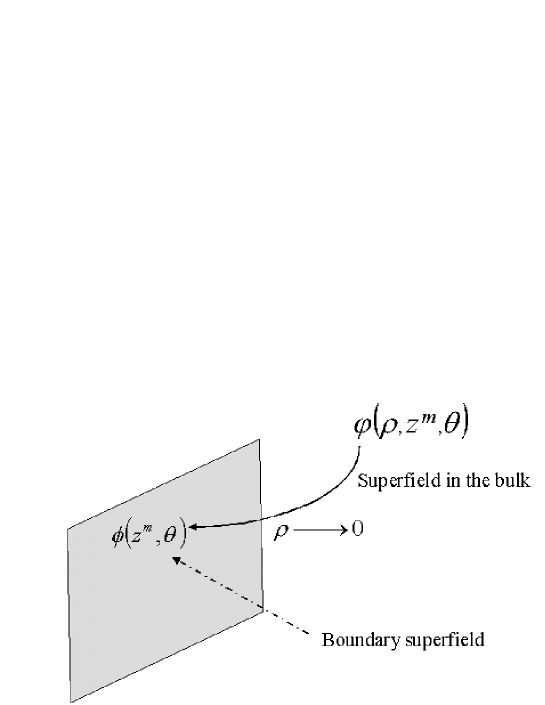
Figure 2: Boundary superfields are obtained as limiting values of superfields in the bulk

The general structure of the $Osp(2|4)$ supermultiplets that may appear in Kaluza Klein supergravity has been determined recently in [29] through consideration of a specific example, that where the manifold $X^{7}$ is the sasakian $M^{1,1,1}$. Performing harmonic analysis on $M^{1,1,1}$ we have found graviton, gravitino and vector multiplets both in a long and in a shortened version. In addition we have found hypermultiplets that are always short and the ultra short multiplets corresponding to massless fields. According to our previous discussion each of these multiplets must correspond to a primary superfield on the boundary. We determine such superfields with the above described method. Short supermultiplets correspond to constrained superfields. The shortening conditions relating mass and hypercharges are retrieved here as the necessary condition to mantain the constraints after a superconformal transformation.

As we anticipated above these primary conformal fields are eventually realized as composite operators in a suitable ${\cal N}=2$, $d=3$ gauge theory. Hence, in the second part of this paper we construct the general form of such a theory. To this effect, rather than superspace formalism we employ our favorite rheonomic approach that, at the end of the day, yields an explicit component form of the lagrangian and the supersymmetry transformation rules for all the physical and auxiliary fields. Although supersymmetric gauge theories in $d=3$ dimensions have been discussed in the literature through many examples (mostly using superspace formalism) a survey of their general form seems to us useful. Keeping track of all the possibilities we construct a supersymmetric off–shell lagrangian that employs all the auxiliary fields and includes, besides minimal gauge couplings and superpotential interactions also Chern Simons interactions and Fayet Iliopoulos terms. We restrict however the kinetic terms of the gauge fields to be quadratic since we are interested in microscopic gauge theories and not in effective lagrangians. Generalization of our results to non minimal couplings including arbitrary holomorphic functions of the scalars in front of the gauge kinetic terms is certainly possible but it is not covered in our paper.

In particular we present general formulae for the scalar potential and we analyse the further conditions that an ${\cal N}=2$ gauge theory should satisfy in order to admit either ${\cal N}=4$ or ${\cal N}=8$ supersymmetry. This is important in connection with the problem of deriving the ultraviolet orbifold gauge theories associated with the sasakian horizons (1.15). Indeed a possible situation that might be envisaged is that where at the orbifold point the gauge theory has larger supersymmetry broken to ${\cal N}=2$ by some of the perturbations responsible for the singularity resolution. It is therefore vital to write ${\cal N}=4$ and ${\cal N}=8$ theories in ${\cal N}=2$ language. This is precisely what we do here.

1.3 Our paper is organized as follows:

In section 2 we discuss the definition and the general properties of the orthosymplectic $Osp({\cal N}|4)$ superalgebra. In particular we discuss its two five–gradings: compact and non compact, the first related to the supergravity interpretation , the second to the superconformal field theory interpretation.

In section 3 we discuss the supercoset structure of superspace and the realization of the $Osp({\cal N}|4)$ superalgebra as an algebra of transformations in two different supercosets, the first describing the bulk of $AdS_{4}$, the second its boundary $\partial(AdS_{4})$.

In section 4 we come to one of the main points of our paper and focusing on the case ${\cal N}=2$ we show how to construct boundary conformal superfields out of the Kaluza Klein $Osp(2|4)$ supermultiplets.

In section 5 we discuss the rheonomic construction of a generic ${\cal N}=2$, $d=3$ gauge theory with arbitrary field content and arbitrary superpotential interactions.

In section 6 we briefly summarize our conclusions.

Finally in appendix A the reader can find the explicit derivation of the Killing vectors generating the action of the $Osp({\cal N}|4)$ superalgebra on superspace. These Killing vectors are an essential tool for the derivation of our result in section 4

2 The $Osp({\cal N}|4)$ superalgebra: definition, properties and notations

The non compact superalgebra $Osp({\cal N}|4)$ relevant to the $AdS_{4}/CFT_{3}$ correspondence is a real section of the complex orthosymplectic superalgebra $Osp({\cal N}|4,\,\hbox{$\vrule height=6.45831pt,width=0.4pt,depth=0.0pt\kern-3.00003pt{\rm C}$})$ that admits the Lie algebra

$$G_{even}=Sp(4,{\rm I\kern-1.79993ptR})\times SO({\cal N},{\rm I\kern-1.79993ptR})$$ (2.1)

as even subalgebra. Alternatively, due to the isomorphism $Sp(4,{\rm I\kern-1.79993ptR})\equiv Usp(2,2)$ we can take a different real section of $Osp({\cal N}|4,\,\hbox{$\vrule height=6.45831pt,width=0.4pt,depth=0.0pt\kern-3.00003pt{\rm C}$})$ such that the even subalgebra is:

$$G_{even}^{\prime}=Usp(2,2)\times SO({\cal N},{\rm I\kern-1.79993ptR})$$ (2.2)

In this paper we mostly rely on the second formulation (2.2) which is more convenient to discuss unitary irreducible representations, while in ([48]) we used the first (2.1) that is more advantageous for the description of the supermembrane geometry. The two formulations are related by a unitary transformation that, in spinor language, corresponds to a different choice of the gamma matrix representation. Formulation (2.1) is obtained in a Majorana representation where all the gamma matrices are real (or purely imaginary), while formulation (2.2) is related to a Dirac representation.

Our choice for the gamma matrices in a Dirac representation is the following one:

$$\Gamma^{0}=\left(\begin{array}[]{cc}\mathord{\!\leavevmode\hbox{ \begin{picture}(0.6,0.7)\put(0.0,0.0){\line(1,0){0.5}} \put(0.15,0.0){\line(0,1){0.7}} \put(0.35,0.0){\line(0,1){0.8}} \put(0.3,0.8){\rule{0.5pt}{0.5pt}}\put(0.26,0.78){\rule{0.5pt}{0.5pt}}\put(0.22,0.76){\rule{0.5pt}{0.5pt}}\put(0.18,0.74){\rule{0.5pt}{0.5pt}}\put(0.14,0.72){\rule{0.5pt}{0.5pt}}\put(0.1,0.7){\rule{0.5pt}{0.5pt}}\put(0.06,0.68){\rule{0.5pt}{0.5pt}}\put(0.02,0.66){\rule{0.5pt}{0.5pt}}\put(-0.02,0.64){\rule{0.5pt}{0.5pt}}\put(-0.06,0.62){\rule{0.5pt}{0.5pt}} \end{picture}}}&0\\ 0&-\mathord{\!\leavevmode\hbox{ \begin{picture}(0.6,0.7)\put(0.0,0.0){\line(1,0){0.5}} \put(0.15,0.0){\line(0,1){0.7}} \put(0.35,0.0){\line(0,1){0.8}} \put(0.3,0.8){\rule{0.5pt}{0.5pt}}\put(0.26,0.78){\rule{0.5pt}{0.5pt}}\put(0.22,0.76){\rule{0.5pt}{0.5pt}}\put(0.18,0.74){\rule{0.5pt}{0.5pt}}\put(0.14,0.72){\rule{0.5pt}{0.5pt}}\put(0.1,0.7){\rule{0.5pt}{0.5pt}}\put(0.06,0.68){\rule{0.5pt}{0.5pt}}\put(0.02,0.66){\rule{0.5pt}{0.5pt}}\put(-0.02,0.64){\rule{0.5pt}{0.5pt}}\put(-0.06,0.62){\rule{0.5pt}{0.5pt}} \end{picture}}}\end{array}\right)\,,\qquad\Gamma^{1,2,3}=\left(\begin{array}[]{cc}0&\tau^{1,2,3}\\ -\tau^{1,2,3}&0\end{array}\right)\,,\qquad C_{[4]}=i\Gamma^{0}\Gamma^{3}\,,$$ (2.3)

having denoted by $C_{[4]}$ the charge conjugation matrix in $4$–dimensions $C_{[4]}\,\Gamma^{\mu}\,C_{[4]}^{-1}=-(\Gamma^{\mu})^{T}$.

Then the $Osp({\cal N}|4)$ superalgebra is defined as the set of graded $(4+{\cal N})\times(4+{\cal N})$ matrices $\mu$ that satisfy the following two conditions:

$$\begin{array}[]{rccclcc}\mu^{T}&\left(\matrix{C_{[4]}&0\cr 0&{\rm 1\kern-3.50006pt1}_{{\cal N}\times{\cal N}}\cr}\right)&+&\left(\matrix{C_{[4]}&0\cr 0&{\rm 1\kern-3.50006pt1}_{{\cal N}\times{\cal N}}\cr}\right)&\mu&=&0\\ \hbox{}\hfil&\hbox{}\hfil&\hbox{}\hfil&\hbox{}\hfil&\hbox{}&\hbox{}\hfil&\hbox{}\hfil\\ \mu^{\dagger}&\left(\matrix{\Gamma^{0}&0\cr 0&-{\rm 1\kern-3.50006pt1}_{{\cal N}\times{\cal N}}\cr}\right)&+&\left(\matrix{\Gamma^{0}&0\cr 0&-{\rm 1\kern-3.50006pt1}_{{\cal N}\times{\cal N}}\cr}\right)&\mu&=&0\\ \end{array}$$ (2.4)

the first condition defining the complex orthosymplectic algebra, the second one the real section with even subalgebra as in eq.(2.2). Eq.s (2.4) are solved by setting:

$$\mu=\left(\matrix{\varepsilon^{AB}\,\frac{1}{4}\,\left[{{\rm I}\kern-1.79993pt\Gamma}_{A}\,,\,{{\rm I}\kern-1.79993pt\Gamma}_{B}\right]&\epsilon^{i}\cr{\bar{\epsilon}}^{i}&\mbox{i}\,\varepsilon_{ij}\,t^{ij}\cr}\right)\\$$

In eq.(2) $\varepsilon_{ij}=-\varepsilon_{ji}$ is an arbitrary real antisymmetric ${\cal N}\times{\cal N}$ tensor, $t^{ij}=-t^{ji}$ is the antisymmetric ${\cal N}\times{\cal N}$ matrix:

$$(t^{ij})_{\ell m}=\mbox{i}\left(\delta^{i}_{\ell}\delta^{j}_{m}-\delta^{i}_{m}\delta^{j}_{\ell}\right)$$ (2.5)

namely a standard generator of the $SO({\cal N})$ Lie algebra,

$${{\rm I}\kern-1.79993pt\Gamma}_{A}=\cases{\begin{array}[]{cl}\mbox{i}\,\Gamma_{5}\Gamma_{\mu}&A=\mu=0,1,2,3\\ \Gamma_{5}\equiv\mbox{i}\Gamma^{0}\Gamma^{1}\Gamma^{2}\Gamma^{3}&A=4\\ \end{array}}$$ (2.6)

denotes a realization of the $SO(2,3)$ Clifford algebra:

$$\left\{{{\rm I}\kern-1.79993pt\Gamma}_{A}\,,\,{{\rm I}\kern-1.79993pt\Gamma}_{B}\right\} = 2\eta_{AB}$$

$$\eta_{AB} = {\rm diag}(+,-,-,-,+)$$ (2.7)

and

$$\epsilon^{i}=C_{[4]}\left({\bar{\epsilon}}^{i}\right)^{T}\quad(i=1,\dots\,{\cal N})$$ (2.8)

are ${\cal N}$ anticommuting Majorana spinors.

The index conventions we have so far introduced can be summarized as follows. Capital indices $A,B=0,1,\ldots,4$ denote $SO(2,3)$ vectors. The latin indices of type $i,j,k=1,\ldots,{\cal N}$ are $SO({\cal N})$ vector indices. The indices $a,b,c,\ldots=1,2,3$ are used to denote spatial directions of $AdS_{4}$: $\eta_{ab}={\rm diag}(-,-,-)$, while the indices of type $m,n,p,\ldots=0,1,2$ are space-time indices for the Minkowskian boundary $\partial\left(AdS_{4}\right)$: $\eta_{mn}={\rm diag}(+,-,-)$. To write the $Osp({\cal N}|4)$ algebra in abstract form it suffices to read the graded matrix (2) as a linear combination of generators:

$$\mu\equiv-\mbox{i}\varepsilon^{AB}\,M_{AB}+\mbox{i}\varepsilon_{ij}\,T^{ij}+{\bar{\epsilon}}_{i}\,Q^{i}$$ (2.9)

where $Q^{i}=C_{[4]}\left(\overline{Q}^{i}\right)^{T}$ are also Majorana spinor operators. Then the superalgebra reads as follows:

$$\left[M_{AB}\,,\,M_{CD}\right] = \mbox{i}\,\left(\eta_{AD}M_{BC}+\eta_{BC}M_{AD}-\eta_{AC}M_{BD}-\eta_{BD}M_{AC}\right)$$

$$\left[T^{ij}\,,\,T^{kl}\right] = -\mbox{i}\,(\delta^{jk}\,T^{il}-\delta^{ik}\,T^{jl}-\delta^{jl}\,T^{ik}+\delta^{il}\,T^{jk})\,$$

$$\left[M_{AB}\,,\,Q^{i}\right] = -\mbox{i}\frac{1}{4}\,\left[{{\rm I}\kern-1.79993pt\Gamma}_{A}\,,\,{{\rm I}\kern-1.79993pt\Gamma}_{B}\right]\,Q^{i}$$

$$\left[T^{ij}\,,\,Q^{k}\right] = -\mbox{i}\,(\delta^{jk}\,Q^{i}-\delta^{ik}\,Q^{j})$$

$$\left\{Q^{\alpha i},\overline{Q}_{\beta}^{\,j}\right\} = \mbox{i}\delta^{ij}\frac{1}{4}\,\left[{{\rm I}\kern-1.79993pt\Gamma}^{A}\,,\,{{\rm I}\kern-1.79993pt\Gamma}^{B}\right]{}^{\alpha}_{\ \beta}M_{AB}+\mbox{i}\delta^{\alpha}_{\,\beta}\,T^{ij}$$ (2.10)

The form (2.10) of the $Osp({\cal N}|4)$ superalgebra coincides with that given in papers [16],[17] and utilized by us in our recent derivation of the $M^{111}$ spectrum [29].

In the gamma matrix basis (2.3) the Majorana supersymmetry charges have the following form:

$$Q^{i}=\left(\matrix{a_{\alpha}^{i}\cr\varepsilon_{\alpha\beta}\bar{a}^{\beta i}}\right)\,,\qquad\bar{a}^{\alpha i}\equiv\left(a_{\alpha}^{i}\right)^{\dagger}\,,$$ (2.11)

where $a_{\alpha}^{i}$ are two-component $SL(2,\,\hbox{$\vrule height=6.45831pt,width=0.4pt,depth=0.0pt\kern-3.00003pt{\rm C}$})$ spinors: $\alpha,\beta,\ldots=1,2$. We do not use dotted and undotted indices to denote conjugate $SL(2,\,\hbox{$\vrule height=6.45831pt,width=0.4pt,depth=0.0pt\kern-3.00003pt{\rm C}$})$ representations; we rather use higher and lower indices. Raising and lowering is performed by means of the $\varepsilon$-symbol:

$$\psi_{\alpha}=\varepsilon_{\alpha\beta}\psi^{\beta}\,,\qquad\psi^{\alpha}=\varepsilon^{\alpha\beta}\psi_{\beta}\,,$$ (2.12)

where $\varepsilon_{12}=\varepsilon^{21}=1$, so that $\varepsilon_{\alpha\gamma}\varepsilon^{\gamma\beta}=\delta_{\alpha}^{\beta}$. Unwritten indeces are contracted according to the rule “from eight to two”.

In the second part of the paper where we deal with the lagrangian of $d=3$ gauge theories, the conventions for two–component spinors are slightly modified to simplify the notations and avoide the explicit writing of spinor indices. The Grassman coordinates of ${\cal N}\!\!=\!\!2$ three-dimensional superspace introduced in equation (4.2) , $\theta^{\pm}_{\alpha}$, are renamed $\theta$ and $\theta^{c}$. The reason for the superscript “$\,{}^{c}\,$” is that, in three dimensions the upper and lower components of the four–dimensional $4$–component spinor are charge conjugate:

$$\theta^{c}\equiv C_{[3]}\overline{\theta}^{T}\,,\qquad\overline{\theta}\equiv\theta^{\dagger}\gamma^{0}\,,$$ (2.13)

where $C_{[3]}$ is the $d=3$ charge conjugation matrix:

$$\left\{\begin{array}[]{ccc}C_{[3]}\gamma^{m}C_{[3]}^{-1}&=&-(\gamma^{m})^{T}\\ \gamma^{0}\gamma^{m}(\gamma^{0})^{-1}&=&(\gamma^{m})^{\dagger}\end{array}\right.$$ (2.14)

The lower case gamma matrices are $2\!\times\!2$ and provide a realization of the $d\!=\!2\!+\!1$ Clifford algebra:

$$\{\gamma^{m}\,,\,\gamma^{n}\}=\eta^{mn}$$ (2.15)

Utilizing the following explicit basis:

$$\left\{\begin{array}[]{ccl}\gamma^{0}&=&\sigma^{2}\\ \gamma^{1}&=&-i\sigma^{3}\\ \gamma^{2}&=&-i\sigma^{1}\end{array}\right.\qquad C_{[3]}=-i\sigma^{2}\,,$$ (2.16)

both $\gamma^{0}$ and $C_{[3]}$ become proportional to $\varepsilon_{\alpha\beta}$. This implies that in equation (2.13) the role of the matrices $C_{[3]}$ and $\gamma^{0}$ is just to convert upper into lower $SL(2,\,\hbox{$\vrule height=6.45831pt,width=0.4pt,depth=0.0pt\kern-3.00003pt{\rm C}$})$ indices and viceversa.

The relation between the two notations for the spinors is summarized in the following table:

$$\begin{array}[]{|c|c|}\hline\cr(\theta^{+})^{\alpha}&\sqrt{2}\,\theta\\ (\theta^{+})_{\alpha}&\sqrt{2}\,\overline{\theta}^{c}\\ (\theta^{-})^{\alpha}&-i\sqrt{2}\,\theta^{c}\\ (\theta^{-})_{\alpha}&-i\sqrt{2}\,\overline{\theta}\\ \hline\cr\end{array}$$ (2.17)

With the second set of conventions the spinor indices can be ignored since the contractions are always made between barred (on the left) and unbarred (on the right) spinors, corresponding to the “eight to two” rule of the first set of conventions. Some examples of this “transcription” are given by:

$$\overline{\theta}\theta={\textstyle\frac{1}{2}}i(\theta^{-})_{\alpha}(\theta^{+})^{\alpha}$$

$$\overline{\theta}^{c}\gamma\theta^{c}={\textstyle\frac{1}{2}}i(\theta^{+})_{\alpha}(\gamma)^{\alpha}_{\ \beta}(\theta^{-})^{\beta}$$ (2.18)

2.1 Compact and non compact five gradings of the $Osp({\cal N}|4)$ superalgebra

As it is extensively explained in [36], a non-compact group $G$ admits unitary irreducible representations of the lowest weight type if it has a maximal compact subgroup $G^{0}$ of the form $G^{0}=H\times U(1)$ with respect to whose Lie algebra $g^{0}$ there exists has a three grading of the Lie algebra $g$ of $G$. In the case of a non–compact superalgebra the lowest weight UIR.s can be constructed if the three grading is generalized to a five grading where the even (odd) elements are integer (half-integer) graded:

$$g=g^{-1}\oplus g^{-{\textstyle\frac{1}{2}}}\oplus g^{0}\oplus g^{+{\textstyle\frac{1}{2}}}\oplus g^{+1}\,,$$ (2.19)

$$\left[g^{k},g^{l}\right]\subset g^{k+l}\qquad g^{k+l}=0\ {\rm for}\ |k+l|>1\,.$$ (2.20)

For the supergroup $Osp({\cal N}|4)$) this grading can be made in two ways, choosing as grade zero subalgebra either the maximal compact subalgebra

$$g^{0}\equiv SO(3)\times SO(2)\times SO({\cal N})\subset Osp({\cal N}|4)$$ (2.21)

or the non-compact subalgebra

$${\widetilde{g}}^{0}\equiv SO(1,2)\times SO(1,1)\times SO({\cal N})\subset Osp({\cal N}|4)$$ (2.22)

which also exists, has the same complex extension and is also maximal.

The existence of the double five–grading is the algebraic core of the $AdS_{4}/CFT_{3}$ correspondence. Decomposing a UIR of $Osp({\cal N}|4)$ into representations of $g^{0}$ shows its interpretation as a supermultiplet of particles states in the bulk of $AdS_{4}$, while decomposing it into representations of ${\widetilde{g}}^{0}$ shows its interpretation as a supermultiplet of conformal primary fields on the boundary $\partial(AdS_{4})$.

In both cases the grading is determined by the generator $X$ of the abelian factor $SO(2)$ or $SO(1,1)$:

$$[X,g^{k}]=k\,g^{k}$$ (2.23)

In the compact case (see [16]) the $SO(2)$ generator $X$ is given by $M_{04}$. It is interpreted as the energy generator of the four-dimensional $AdS$ theory. It was used in [17] and [29] for the construction of the $Osp(2|4)$ representations, yielding the long multiplets of [17] and the short and ultra-short multiplets of [29]. We repeat such decompositions here.

We call $E$ the energy generator of $SO(2)$, $L_{a}$ the rotations of $SO(3)$:

$$E = M_{04}\,,$$

$$L_{a} = {\textstyle\frac{1}{2}}\varepsilon_{abc}\,M_{bc}\,,$$ (2.24)

and $M_{a}^{\pm}$ the boosts:

$$M_{a}^{+} = -M_{a4}+iM_{0a}\,,$$

$$M_{a}^{-} = M_{a4}+iM_{0a}\,.$$ (2.25)

The supersymmery generators are $a^{i}_{\alpha}$ and $\bar{a}^{\alpha i}$. Rewriting the $Osp({\cal N}|4)$ superalgebra (2.10) in this basis we obtain:

$${}[E,M_{a}^{+}] = M_{a}^{+}\,,$$

$${}[E,M_{a}^{-}] = -M_{a}^{-}\,,$$

$${}[L_{a},L_{b}] = i\,\varepsilon_{abc}L_{c}\,,$$

$${}[M^{+}_{a},M^{-}_{b}] = 2\,\delta_{ab}\,E+2i\,\varepsilon_{abc}\,L_{c}\,,$$

$${}[L_{a},M^{+}_{b}] = i\,\varepsilon_{abc}\,M^{+}_{c}\,,$$

$${}[L_{a},M^{-}_{b}] = i\,\varepsilon_{abc}\,M^{-}_{c}\,,$$

$${}[T^{ij},T^{kl}] = -i\,(\delta^{jk}\,T^{il}-\delta^{ik}\,T^{jl}-\delta^{jl}\,T^{ik}+\delta^{il}\,T^{jk})\,,$$

$${}[T^{ij},\bar{a}^{\alpha k}] = -i\,(\delta^{jk}\,\bar{a}^{\alpha i}-\delta^{ik}\,\bar{a}^{\alpha j})\,,$$

$${}[T^{ij},a_{\alpha}^{k}] = -i\,(\delta^{jk}\,a_{\alpha}^{i}-\delta^{ik}\,a_{\alpha}^{i})\,,$$

$${}[E,a_{\alpha}^{i}] = -{\textstyle\frac{1}{2}}\,a_{\alpha}^{i}\,,$$

$${}[E,\bar{a}^{\alpha i}] = {\textstyle\frac{1}{2}}\,\bar{a}^{\alpha i}\,,$$

$${}[M_{a}^{+},a_{\alpha}^{i}] = (\tau_{a})_{\alpha\beta}\,\bar{a}^{\beta i}\,,$$

$${}[M_{a}^{-},\bar{a}^{\alpha i}] = -(\tau_{a})^{\alpha\beta}\,a_{\beta}^{i}\,,$$

$${}[L_{a},a_{\alpha}^{i}] = {\textstyle\frac{1}{2}}\,(\tau_{a})_{\alpha}{}^{\beta}\,a^{i}_{\beta}\,,$$

$${}[L_{a},\bar{a}^{\alpha i}] = -{\textstyle\frac{1}{2}}\,(\tau_{a})^{\alpha}{}_{\beta}\,\bar{a}^{\beta i}\,,$$

$$\{a_{\alpha}^{i},a_{\beta}^{j}\} = \delta^{ij}\,(\tau^{k})_{\alpha\beta}\,M_{k}^{-}\,,$$

$$\{\bar{a}^{\alpha i},\bar{a}^{\beta j}\} = \delta^{ij}(\tau^{k})^{\alpha\beta}\,M_{k}^{+}\,,$$

$$\{a_{\alpha}^{i},\bar{a}^{\beta j}\} = \delta^{ij}\,\delta_{\alpha}{}^{\beta}\,E+\delta^{ij}\,(\tau^{k})_{\alpha}{}^{\beta}\,L_{k}+i\,\delta_{\alpha}{}^{\beta}\,T^{ij}\,.$$ (2.26)

The five–grading structure of the algebra (2.26) is shown in fig. 3 In the superconformal field theory context we are interested in the action of the $Osp({\cal N}|4)$ generators on superfields living on the minkowskian boundary $\partial(AdS_{4})$. To be precise the boundary is a compactification of $d=3$ Minkowski space and admits a conformal family of metrics $g_{mn}=\phi(z)\eta_{mn}$ conformally equivalent to the the flat Minkowski metric

$$\eta_{mn}=(+,-,-)\,,\qquad m,n,p,q=0,1,2\,.$$ (2.27)

Precisely because we are interested in conformal field theories the the choice of representative metric inside the conformal family is immaterial and the flat one (2.27) is certainly the most convenient. The requested action of the superalgebra generators is obtained upon starting from the non–compact grading with respect to (2.22). To this effect we define the dilatation $SO(1,1)$ generator $D$ and the Lorentz $SO(1,2)$ generators $J^{m}$ as follows:

$$D\equiv i\,M_{34}\,,\qquad J^{m}={\textstyle\frac{i}{2}}\,\varepsilon^{mpq}M_{pq}\,.$$ (2.28)

Figure 3: Schematic representation of the root diagram of $Osp({\cal N}|4)$ in the $SO(2)\times SO(3)$ basis. The grading w.r.t. the energy $E$ is given on the right.

In addition we define the the $d=3$ translation generators $P_{m}$ and special conformal boosts $K_{m}$ as follows:

$$P_{m}=M_{m4}-M_{3m}\,,$$

$$K_{m}=M_{m4}+M_{3m}\,.$$ (2.29)

Finally we define the generators of $d=3$ ordinary and special conformal supersymmetries, respectively given by:

$$q^{\alpha i}={\textstyle\frac{1}{\sqrt{2}}}\left(a_{\alpha}^{i}+\bar{a}^{\alpha i}\right)\,,$$

$$s_{\alpha}^{i}={\textstyle\frac{1}{\sqrt{2}}}\left(-a_{\alpha}^{i}+\bar{a}^{\alpha i}\right)\,.$$ (2.30)

The $SO({\cal N})$ generators are left unmodified as above. In this new basis the $Osp({\cal N}|4)$-algebra (2.10) reads as follows

$${}[D,P_{m}] = -P_{m}\,,$$

$${}[D,K_{m}] = K_{m}\,,$$

$${}[J_{m},J_{n}] = \varepsilon_{mnp}\,J^{p}\,,$$

$${}[K_{m},P_{n}] = 2\,\eta_{mn}\,D-2\,\varepsilon_{mnp}\,J^{p}\,,$$

$${}[J_{m},P_{n}] = \varepsilon_{mnp}\,P^{p}\,,$$

$${}[J_{m},K_{n}] = \varepsilon_{mnp}\,K^{p}\,,$$

$${}[T^{ij},T^{kl}] = -i\,(\delta^{jk}\,T^{il}-\delta^{ik}\,T^{jl}-\delta^{jl}\,T^{ik}+\delta^{il}\,T^{jk})\,,$$

$${}[T^{ij},q^{\alpha k}] = -i\,(\delta^{jk}\,q^{\alpha i}-\delta^{ik}\,q^{\alpha j})\,,$$

$${}[T^{ij},s_{\alpha}^{k}] = -i\,(\delta^{jk}\,s_{\alpha}^{i}-\delta^{ik}\,s_{\alpha}^{i})\,,$$

$${}[D,q^{\alpha i}] = -{\textstyle\frac{1}{2}}\,q^{\alpha i}\,,$$

$${}[D,s_{\alpha}^{i}] = {\textstyle\frac{1}{2}}\,s_{\alpha}^{i}\,,$$

$${}[K^{m},q^{\alpha i}] = -i\,(\gamma^{m})^{\alpha\beta}\,s_{\beta}^{i}\,,$$

$${}[P^{m},s_{\alpha}^{i}] = -i\,(\gamma^{m})_{\alpha\beta}\,q^{\beta i}\,,$$

$${}[J^{m},q^{\alpha i}] = -{\textstyle\frac{i}{2}}\,(\gamma^{m})^{\alpha}{}_{\beta}q^{\beta i}\,,$$

$${}[J^{m},s_{\alpha}^{i}] = {\textstyle\frac{i}{2}}\,(\gamma^{m})_{\alpha}{}^{\beta}s_{\beta}^{i}\,,$$

$$\{q^{\alpha i},q^{\beta j}\} = -i\,\delta^{ij}\,(\gamma^{m})^{\alpha\beta}P_{m}\,,$$

$$\{s_{\alpha}^{i},s_{\beta}^{j}\} = i\,\delta^{ij}\,(\gamma^{m})_{\alpha\beta}K_{m}\,,$$

$$\{q^{\alpha i},s_{\beta}^{j}\} = \delta^{ij}\delta^{\alpha}{}_{\beta}\,D-i\,\delta^{ij}(\gamma^{m})^{\alpha}{}_{\beta}J_{m}+i\delta^{\alpha}{}_{\beta}T^{ij}\,.$$ (2.31)

and the five grading structure of eq.s (2.31) is displayed in fig.4.

Figure 4: Schematic representation of the root diagram of $Osp({\cal N}|4)$ in the $SO(1,1)\times SO(1,2)$ basis. The grading w.r.t. the dilatation $D$ is given on the right.

In both cases of fig.3 and fig.4 if one takes the subset of generators of positive grading plus the abelian grading generator $X=\cases{E\cr D\cr}$ one obtains a solvable superalgebra of dimension $4+2{\cal N}$. It is however only in the non compact case of fig.4 that the bosonic subalgebra of the solvable superalgebra generates anti de Sitter space $AdS_{4}$ as a solvable group manifold. Therefore the solvable superalgebra $Ssolv_{adS}$ mentioned in eq. (1.20) is the vector span of the following generators:

$$Ssolv_{adS}\equiv\mbox{span}\left\{P_{m},D,q^{\alpha i}\right\}$$ (2.32)

2.2 The lowest weight UIR.s as seen from the compact and non compact five–grading viewpoint

The structure of all the $Osp(2|4)$ supermultiplets relevant to Kaluza Klein supergravity is known. Their spin content is upper bounded by $s=2$ and they fall into three classes: long, short and ultrashort. Such a result has been obtained in [29] by explicit harmonic analysis on $X^{7}=M^{111}$, namely through the analysis of a specific example of ${\cal N}\!\!=\!\!2$ compactification on $AdS_{4}\times X^{7}$. As stressed in the introduction the goal of the present paper is to reformulate the structure of these multiplets in a way appropriate for comparison with composite operators of the three-dimensional gauge theory living on the boundary $\partial(AdS_{4})$ that behave as primary conformal fields. Actually, in view of the forthcoming Kaluza-Klein spectrum on $X^{7}=N^{010}$ [42], that is arranged into $Osp(3|4)$ rather than $Osp(2|4)$ multiplets, it is more convenient to begin by discussing $Osp({\cal N}|4)$ for generic ${\cal N}$.

We start by briefly recalling the procedure of [16, 43] to construct UIR.s of $Osp({\cal N}|4)$ in the compact grading (2.21). Then, in a parallel way to what was done in [37] for the case of the $SU(2,2|4)$ superalgebra we show that also for $Osp({\cal N}|4)$in each UIR carrier space there exists a unitary rotation that maps eigenstates of $E,L^{2},L_{3}$ into eigenstates of $D,J^{2},J_{2}$. By means of such a rotation the decomposition of the UIR into $SO(2)\times SO(3)$ representations is mapped into an analogous decomposition into $SO(1,1)\times SO(1,2)$ representations. While $SO(2)\times SO(3)$ representations describe the on–shell degrees of freedom of a bulk particle with an energy $E_{0}$ and a spin $s$, irreducible representations of $SO(1,1)\times SO(1,2)$ describe the off-shell degrees of freedom of a boundary field with scaling weight $D$ and Lorentz character $J$. Relying on this we show how to construct the on-shell four-dimensional superfield multiplets that generate the states of these representations and the off-shell three-dimensional superfield multiplets that build the conformal field theory on the boundary.

Lowest weight representations of $Osp({\cal N}|4)$ are constructed starting from the basis (2.26) and choosing a a vacuum state such that

$$M_{i}^{-}|(E_{0},s,\Lambda)\rangle = 0\,,$$

$$a^{i}_{\alpha}|(E_{0},s,\Lambda)\rangle = 0\,,$$ (2.33)

where $E_{0}$ denotes the eigenvalue of the energy operator $M_{04}$ while $s$ and $\Lambda$ are the labels of an irreducible $SO(3)$ and $SO({\cal N})$ representation, respectively. In particular we have:

$$M_{04}\,|(E_{0},s,\Lambda)\rangle = E_{0}\,|(E_{0},s,\Lambda)\rangle$$

$$L^{a}\,L^{a}\,|(E_{0},s,\Lambda)\rangle = s(s+1)\,|(E_{0},s,\Lambda)\rangle$$

$$L^{3}|(E_{0},s,\Lambda)\rangle = s\,|(E_{0},s,\Lambda)\rangle\,.$$ (2.34)

The states filling up the UIR are then built by applying the operators $M^{-}$ and the anti-symmetrized products of the operators $\bar{a}^{i}_{\alpha}$:

$$\left(M_{1}^{+}\right)^{n_{1}}\left(M_{2}^{+}\right)^{n_{2}}\left(M_{3}^{+}\right)^{n_{3}}[\bar{a}^{i_{1}}_{\alpha_{1}}\dots\bar{a}^{i_{p}}_{\alpha_{p}}]|(E_{0},s,\Lambda)\rangle$$ (2.35)

Lowest weight representations are similarly constructed with respect to five–grading (2.31). One starts from a vacuum state that is annihilated by the conformal boosts and by the special conformal supersymmetries

$$K_{m}\,|(D_{0},j,\Lambda)\rangle = 0\,,$$

$$s^{i}_{\alpha}\,|(D_{0},j,\Lambda)\rangle = 0\,,$$ (2.36)

and that is an eigenstate of the dilatation operator $D$ and an irreducible $SO(1,2)$ representation of spin $j$:

$$D\,|(D_{0},j,\Lambda)\rangle = D_{0}\,|(D_{0},j,\Lambda)\rangle$$

$$J^{m}\,J^{n}\,\eta_{mn}\,|(D_{0},j,\Lambda)\rangle = j(j+1)\,|(D_{0},j,\Lambda)\rangle$$

$$J_{2}\,|(D_{0},j,\Lambda)\rangle = j|(D_{0},j,\Lambda)\rangle$$ (2.37)

As for the $SO({\cal N})$ representation the new vacuum is the same as before. The states filling the UIR are now constructed by applying to the vacuum the operators $P_{m}$ and the anti-symmetrized products of $q^{\alpha i}$,

$$\left(P_{0}\right)^{p_{0}}\left(P_{1}\right)^{p_{1}}\left(P_{2}\right)^{p_{2}}[q^{\alpha_{1}i_{1}}\dots q^{\alpha_{q}i_{q}}]|(D_{0},j,\Lambda)\rangle\,.$$ (2.38)

In the language of conformal field theories the vacuum state satisfying eq.(2.36) is named a primary state (corresponding to the value at $z^{m}=0$ of a primary conformal field. The states (2.38) are called the descendants.

The rotation between the $SO(3)\times SO(2)$ basis and the $SO(1,2)\times SO(1,1)$ basis is performed by the operator:

$$U\equiv\exp\left[{{\textstyle\frac{i}{\sqrt{2}}}\pi(E-D)}\right]\,,$$ (2.39)

which has the following properties,

$$DU = -UE\,,$$

$$J_{0}U = i\,UL_{3}\,,$$

$$J_{1}U = UL_{1}\,,$$

$$J_{2}U = UL_{2}\,,$$ (2.40)

with respect to the grade $0$ generators. Furthermore, with respect to the non vanishing grade generators we have:

$$K_{0}U = -i\,UM_{3}^{-}\,,$$

$$K_{1}U = -UM_{1}^{-}\,,$$

$$K_{2}U = -UM_{2}^{-}\,,$$

$$P_{0}U = i\,UM_{3}^{+}\,,$$

$$P_{1}U = UM_{1}^{+}\,,$$

$$P_{2}U = UM_{2}^{+}\,,$$

$$q^{\alpha i}U = -i\,U\bar{a}^{\alpha i}$$

$$s_{\alpha}^{i}U = i\,Ua_{\alpha}^{i}\,.$$ (2.41)

As one immediately sees from (2.41), U interchanges the compact five–grading structure of the superalgebra with its non compact one. In particular the $SO(3)\times SO(2)$-vacuum with energy $E_{0}$ is mapped into an $SO(1,2)\times SO(1,1)$ primary state and one obtains all the descendants (2.38) by acting with $U$ on the particle states (2.35). Furthermore from (2.40) we read the conformal weight and the Lorentz group representation of the primary state $U|(E_{0},s,J)\rangle$. Indeed its eigenvalue with respect to the dilatation generator $D$ is:

$$D_{0}=-E_{0}\,.$$ (2.42)

and we find the following relation between the Casimir operators of $SO(1,2)$ and $SO(3)$,

$$J^{2}U=UL^{2}\,,\qquad J^{2}\equiv-J_{0}^{2}+J_{1}^{2}+J_{2}^{2}\,,$$ (2.43)

which implies that

$$j=s\,.$$ (2.44)

Hence under the action of $U$ a particle state of energy $E_{0}$ and spin $s$ of the bulk is mapped into a primary conformal field of conformal weight $-E_{0}$ and Lorentz spin $s$ on the boundary. This discussion is visualized in fig.5

Figure 5: The operator $U=\exp\{i\pi/\sqrt{2}(E-D)\}$ rotates the Hilbert space of the physical states. It takes states labeled by the Casimirs ($E,\,s$) of the $SO(2)\times SO(3)\subset Osp({\cal N}|4)$ into states labeled by the Casimirs ($D,\,j$) of $SO(1,1)\times SO(1,2)$.

3 $AdS_{4}$ and $\partial AdS_{4}$ as cosets and their Killing vectors

In the previous section we studied $Osp({\cal N}|4)$ and its representations in two different bases. The form (2.26) of the superalgebra is that we used in [29] to construct the $Osp(2|4)$ supermultiplets from Kaluza Klein supergravity. It will be similarly used to obtain the $Osp(3|4)$ spectrum on $X^{7}=N^{010}$. We translated these results in terms of the form (2.31) of the $Osp({\cal N}|4)$ algebra in order to allow a comparison with the three-dimensional CFT on the boundary. In this section we introduce the announced description of the anti de Sitter superspace and of its boundary in terms of supersolvable Lie algebra parametrization as in eq.s(1.20),(1.21). It turns out that such a description is the most appropriate for a comparative study between $AdS_{4}$ and its boundary. We calculate the Killing vectors of these two coset spaces since they are needed to determine the superfield multiplets living on both $AdS_{4}$ and $\partial AdS_{4}$.

So we write both the bulk and the boundary superspaces as supercosets,

$$\frac{G}{H}\,,$$ (3.1)

Applying supergroup elements $g\in Osp({\cal N}|4)$ to the coset representatives $L(y)$ these latter transform as follows:

$$g\,L(y)=L(y^{\prime})h(g,y)\,,$$ (3.2)

where $h(y)$ is some element of $H\subset Osp({\cal N}|4)$, named the compensator that, generically depends both on $g$ and on the coset point $y\in G/H$. For our purposes it is useful to consider the infinitesimal form of (3.2), i.e. for infinitesimal $g$ we can write:

$$g = 1+\epsilon^{A}T_{A}\,,$$

$$h = 1+\epsilon^{A}W^{H}_{A}(y)T_{H}\,,$$

$$y^{\mu\prime}\, = y^{\mu}+\epsilon^{A}k^{\mu}_{A}(y)$$ (3.3)

and we obtain:

$$T_{A}L(y) = k_{A}L(y)+L(y)T_{H}W^{H}_{A}(y)\,,$$ (3.4)

$$k_{A} \equiv k^{\mu}_{A}(y)\,\frac{\partial}{\partial y^{\mu}}$$ (3.5)

The shifts in the superspace coordinates $y$ determined by the supergroup elements (see eq.(3.2)) define the Killing vector fields (3.5) of the coset manifold.

Let us now consider the solvable anti de Sitter superspace defined in eq.s (1.20),(1.21). It describes a $\kappa$–gauge fixed supersymmetric extension of the bulk $AdS_{4}$. As explained by eq.(1.21) it is a supercoset (3.1) where $G=Osp({\cal N}|4)$ and $H=CSO(1,2|{\cal N})\times SO({\cal N})$ Using the non–compact basis (2.31), the subgroup $H$ is given by,

$$H^{AdS}=CSO(1,2|{\cal N})\,\equiv\,\mbox{span}\,\left\{\,J^{m},K_{m},s_{\alpha}^{i},T^{ij}\,\right\}\,.$$ (3.6)

A coset representative can be written as follows:

$$L^{AdS}(y)=\exp\left[{\rho D+i\,x\cdot P+\theta^{i}q^{i}}\right]\,,\qquad y=(\rho,x,\theta)\,.$$ (3.7)

In $AdS_{4|2{\cal N}}$ $s$-supersymmetry and $K$-symmetry have a non linear realization since the corresponding generators are not part of the solvable superalgebra $Ssolv_{adS}$ that is exponentiated (see eq.(2.32).

The form of the Killing vectors simplifies considerably if we rewrite the coset representative as a product of exponentials

$$L(y)=\exp\left[i\,z\cdot P\right]\,\cdot\,\exp\left[\xi^{i}q^{i}\right]\,\cdot\,\exp\left[{\rho D}\right]$$ (3.8)

This amounts to the following coordinate change:

$$z = \left(1-{\textstyle\frac{1}{2}}\rho+{\textstyle\frac{1}{6}}\rho^{2}+{\cal O}(\rho^{3})\right)\,x\,,$$

$$\xi^{i} = \left(1-{\textstyle\frac{1}{4}}\rho+{\textstyle\frac{1}{24}}\rho^{2}+{\cal O}(\rho^{3})\right)\,\theta^{i}\,.$$ (3.9)

This is the parametrization that was used in [48] to get the $Osp(8|4)$-singleton action from the supermembrane. For this choice of coordinates the anti de Sitter metric takes the standard form (1.9). The Killing vectors are

$$\stackrel{{\scriptstyle\rightarrow}}{{k}}[P_{m}] = -i\,\partial_{m}\,,$$

$$\stackrel{{\scriptstyle\rightarrow}}{{k}}[q^{\alpha i}] = \frac{\partial}{\partial\xi_{\alpha}^{i}}-\frac{1}{2}\left(\gamma^{m}\xi^{i}\right)^{\alpha}\partial_{m}\,,$$

$$\stackrel{{\scriptstyle\rightarrow}}{{k}}[J^{m}] = \varepsilon^{mpq}z_{p}\partial_{q}-\frac{i}{2}\left(\xi^{i}\gamma^{m}\right)_{\alpha}\frac{\partial}{\partial\xi_{\alpha}^{i}}\,,$$

$$\stackrel{{\scriptstyle\rightarrow}}{{k}}[D] = \frac{\partial}{\partial\rho}-z\cdot\partial-\frac{1}{2}\xi_{\alpha}^{i}\frac{\partial}{\partial\xi_{\alpha}^{i}}\,,$$

$$\stackrel{{\scriptstyle\rightarrow}}{{k}}[s^{\alpha i}] = -\xi^{\alpha i}\frac{\partial}{\partial\rho}+\frac{1}{2}\xi^{\alpha i}\,z\cdot\partial+\frac{i}{2}\varepsilon^{pqm}\,z_{p}(\gamma_{q}\xi^{i})^{\alpha}\partial_{m}$$ (3.10)

$$-\frac{1}{8}(\xi^{j}\xi^{j})(\gamma^{m}\xi^{i})^{\alpha}\partial_{m}-z^{m}(\gamma_{m})^{\alpha}{}_{\beta}\frac{\partial}{\partial\xi^{i}_{\beta}}-\frac{1}{4}(\xi^{j}\xi^{j})\frac{\partial}{\partial\xi^{i}_{\alpha}}$$

$$+\frac{1}{2}\xi^{\alpha i}\xi^{\beta j}\frac{\partial}{\partial\xi^{j}_{\beta}}-\frac{1}{2}(\gamma^{m}\xi^{i})^{\alpha}\xi^{j}_{\beta}\gamma_{m}\frac{\partial}{\partial\xi^{j}_{\beta}}\,.$$

and for the compensators we find:

$$W[P] = 0\,,$$

$$W[q^{\alpha i}] = 0\,,$$

$$W[J^{m}] = J^{m}\,,$$

$$W[D] = 0\,,$$

$$W[s^{\alpha i}] = s^{\alpha i}-i\,\left(\gamma^{m}\theta^{i}\right)^{\alpha}\,J_{m}+i\theta^{\alpha j}\,T^{ij}\,.$$ (3.11)

For a detailed derivation of these Killing vectors and compensators we refer the reader to appendix A.

The boundary superspace $\partial(AdS_{4|2{\cal N}})$ is formed by the points on the supercoset with $\rho=0$:

$$L^{CFT}(y)=\exp\left[\mbox{ i}\,x\cdot P+\theta^{i}q^{i}\right]$$ (3.12)

In order to see how the supergroup acts on fields that live on this boundary we use the fact that this submanifold is by itself a supercoset. Indeed instead of $H^{AdS}\subset Osp({\cal N}|4)$ as given in (3.6), we can choose the larger subalgebra

$$H^{CFT}=\mbox{span}\,\left\{D,J^{m},K_{m},s_{\alpha}^{i},T^{ij}\right\}\,.$$ (3.13)

and consider the new supercoset $G/H^{CFT}$. By defintion also on this smaller space we have a non linear realization of the full orthosymplectic superalgebra. For the Killing vectors we find:

$$\stackrel{{\scriptstyle\rightarrow}}{{k}}[P_{m}] = -i\,\partial_{m}\,,$$

$$\stackrel{{\scriptstyle\rightarrow}}{{k}}[q^{\alpha i}] = \frac{\partial}{\partial\theta_{\alpha}^{i}}-\frac{1}{2}\left(\gamma^{m}\theta^{i}\right)^{\alpha}\partial_{m}\,,$$

$$\stackrel{{\scriptstyle\rightarrow}}{{k}}[J^{m}] = \varepsilon^{mpq}x_{p}\partial_{q}-\frac{i}{2}\left(\theta^{i}\gamma^{m}\right)_{\alpha}\frac{\partial}{\partial\theta_{\alpha}^{i}}\,,$$

$$\stackrel{{\scriptstyle\rightarrow}}{{k}}[D] = -x\cdot\partial-\frac{1}{2}\theta_{\alpha}^{i}\frac{\partial}{\partial\theta_{\alpha}^{i}}\,,$$

$$\stackrel{{\scriptstyle\rightarrow}}{{k}}[s^{\alpha i}] = \frac{1}{2}\theta^{\alpha i}\,x\cdot\partial+\frac{i}{2}\varepsilon^{pqm}\,x_{p}(\gamma_{q}\theta^{i})^{\alpha}\partial_{m}-\frac{1}{8}(\theta^{j}\theta^{j})(\gamma^{m}\theta^{i})^{\alpha}\partial_{m}$$

$$-x^{m}(\gamma_{m})^{\alpha}{}_{\beta}\frac{\partial}{\partial\theta^{i}_{\beta}}-\frac{1}{4}(\theta^{j}\theta^{j})\frac{\partial}{\partial\theta^{i}_{\alpha}}+\frac{1}{2}\theta^{\alpha i}\theta^{\beta j}\frac{\partial}{\partial\theta^{j}_{\beta}}-\frac{1}{2}(\gamma^{m}\theta^{i})^{\alpha}\theta^{j}_{\beta}\gamma_{m}\frac{\partial}{\partial\theta^{j}_{\beta}}\,.$$

and for the compensators we have:

$$W[P_{m}] = 0\,,$$

$$W[q^{\alpha i}] = 0\,,$$

$$W[J^{m}] = J^{m}\,,$$

$$W[D] = D\,,$$

$$W[s^{\alpha i}] = -\theta^{\alpha i}\,D+s^{\alpha i}-i\,\left(\gamma^{m}\theta^{i}\right)^{\alpha}\,J_{m}+i\theta^{j}T^{ij}\,.$$ (3.15)

If we compare the Killing vectors on the boundary (LABEL:bounkil) with those on the bulk (3.10) we see that they are very similar. The only formal difference is the suppression of the $\frac{\partial}{\partial\rho}$ terms. The conceptual difference, however, is relevant. On the boundary the transformations generated by (LABEL:bounkil) are the standard superconformal transformations in three–dimensional (compactified) Minkowski space. In the bulk the transformations generated by (3.10) are superisometries of anti de Sitter superspace. They might be written in completely different but equivalent forms if we used other coordinate frames. The form they have is due to the use of the solvable coordinate frame $(\rho,z,\xi)$ which is the most appropriate to study the restriction of bulk supermultiplets to the boundary. For more details on this point we refer the reader to appendix A

4 $Osp(2|4)$ superfields in the bulk and on the boundary

As we explained in the introduction our main goal is the determination of the ${\cal N}=2$ three dimensional gauge theories associated with the sasakian horizons (1.15) and the comparison between Kaluza Klein spectra of M–theory compactified on $AdS_{4}$ times such horizons with the spectrum of primary conformal superfields of the corresponding gauge theory. For this reason we mainly focus on the case of $Osp(2|4)$ supermultiplets. As already stressed the structure of such supermultiplets has been determined in Kaluza Klein language in [17, 29]. Hence they have been obtained in the basis (2.26) of the orthosymplectic superalgebra. Here we consider their translation into the superconformal language provided by the other basis (2.31). In this way we will construct a boundary superfield associated with each particle supermultiplet of the bulk. The components of the supermultiplet are Kaluza Klein states: it follows that we obtain a one–to–one correspondence between Kaluza Klein states and components of the boundary superfield.

4.1 Conformal $Osp(2|4)$ superfields: general discussion

So let us restrict our attention to ${\cal N}\!\!=\!\!2$. In this case the $SO(2)$ group has just one generator that we name the hypercharge:

$$Y\equiv T^{21}\,.$$ (4.1)

Since it is convenient to work with eigenstates of the hypercharge operator, we reorganize the two Grassman spinor coordinates of superspace in complex combinations:

$$\theta^{\pm}_{\alpha}=\frac{1}{\sqrt{2}}(\theta^{1}_{\alpha}\pm i\theta^{2}_{\alpha})\,,\qquad Y\,\theta^{\pm}_{\alpha}=\pm\theta^{\pm}_{\alpha}$$ (4.2)

In this new notations the Killing vectors generating $q$–supersymmetries on the boundary (see eq.(LABEL:bounkil)) take the form:

$${\vec{k}}\left[q^{\alpha i}\right]\quad\longrightarrow\quad q^{\alpha\pm}=\frac{\partial}{\partial\theta^{\mp}_{\alpha}}-{\textstyle\frac{1}{2}}\,(\gamma^{m})^{\alpha}{}_{\beta}\theta^{\beta\pm}\partial_{m}\,,$$ (4.3)

A generic superfield is a function $\Phi(x,\theta)$ of the bosonic coordinates $x$ and of all the $\theta.s$ Expanding such a field in power series of the $\theta.s$ we obtain a multiplet of $x$–space fields that, under the action of the Killing vector (4.3), form a representation of Poincaré supersymmetry. Such a representation can be shortened by imposing on the superfield $\Phi(x,\theta)$ constraints that are invariant with respect to the action of the Killing vectors (4.3). This is possible because of the existence of the so called superderivatives, namely of fermionic vector fields that commute with the supersymmetry Killing vectors. In our notations the superderivatives are defined as follows:

$${\cal D}^{\alpha\pm}=\frac{\partial}{\partial\theta^{\mp}_{\alpha}}+{\textstyle\frac{1}{2}}\,(\gamma^{m})^{\alpha}{}_{\beta}\theta^{\beta\pm}\partial_{m}\,,$$ (4.4)

and satisfy the required property

$$\begin{array}[]{rclcr}\{{\cal D}^{\alpha\pm},q^{\beta\pm}\}&=&\{{\cal D}^{\alpha\pm},q^{\beta\mp}\}&=&0\,.\end{array}$$ (4.5)

As explained in [44] the existence of superderivatives is the manifestation at the fermionic level of a general property of coset manifolds. For $G/H$ the true isometry algebra is not $G$, rather it is $G\times N(H)_{G}$ where $N(H)_{G}$ denotes the normalizer of the stability subalgebra $H$. The additional isometries are generated by right–invariant rather than left–invariant vector fields that as such commute with the left–invariant ones. If we agree that the Killing vectors are left–invariant vector fields than the superderivatives are right–invariant ones and generate the additional superisometries of Poincaré superspace. Shortened representations of Poincaré supersymmetry are superfields with a prescribed behaviour under the additional superisometries: for instance they may be invariant under such transformations. We can formulate these shortening conditions by writing constraints such as

$${\cal D}^{\alpha+}\Phi(x,\theta)=0\,.$$ (4.6)

The key point in our discussion is that a constraint of type (4.6) is guaranteed from eq.s (4.5) to be invariant with respect to the superPoincaré algebra, yet it is not a priori guaranteed that it is invariant under the action of the full superconformal algebra (LABEL:bounkil). Investigating the additional conditions that make a constraint such as (4.6) superconformal invariant is the main goal of the present section. This is the main tool that allows a transcription of the Kaluza–Klein results for supermultiplets into a superconformal language.

To develop such a programme it is useful to perform a further coordinate change that is quite traditional in superspace literature. Given the coordinates $x$ on the boundary (or the coordinates $z$ for the bulk) we set:

$$y^{m}=x^{m}+{\textstyle\frac{1}{2}}\,\theta^{+}\gamma^{m}\theta^{-}\,.$$ (4.7)

Then the superderivatives become

$${\cal D}^{\alpha+} = \frac{\partial}{\partial\theta^{-}_{\alpha}}\,,$$

$${\cal D}^{\alpha-} = \frac{\partial}{\partial\theta^{+}_{\alpha}}+(\gamma^{m})^{\alpha}{}_{\beta}\theta^{\beta-}\partial_{m}\,.$$ (4.8)

It is our aim to describe superfield multiplets both on the bulk and on the boundary. It is clear that one can do the same redefinitions for the Killing vector of $q$-supersymmetry (4.3) and that one can introduce superderivatives also for the theory on the bulk. In that case one inserts the functions $t(\rho)$ and $\gamma(\rho)$ in the above formulas or if one uses the solvable coordinates $(\rho,z,\xi)$ as in (3.9) then there is just no difference with the boundary case.

So let us finally turn to superfields. We begin by focusing on boundary superfields since their treatment is slightly easier than the treatment of bulk superfields.

Definition 4.1

A primary superfield is defined as follows (see [37, 47]),

$$\Phi^{\partial AdS}(x,\theta)=\exp\left[\mbox{i}\,x\cdot P+\theta^{i}q^{i}\right]\Phi(0)\,,$$ (4.9)

where $\Phi(0)$ is a primary state (see eq.(2.36))

$$s_{\alpha}^{i}\Phi(0) = 0\,,$$

$$K_{m}\Phi(0) = 0\,.$$ (4.10)

of scaling weight $D_{0}$, hypercharge $y_{0}$ and eigenvalue $j$ for the “third-component” operator $J_{2}$

$$\begin{array}[]{ccccc}D\,\Phi(0)=D_{0}\,\Phi(0)&;&Y\,\Phi(0)=y_{0}\,\Phi(0)&;&J_{2}\,\Phi(0)=j\,\Phi(0)\end{array}$$ (4.11)

From the above defintion one sees that the primary superfield $\Phi^{\partial AdS}(x,\theta)$ is actually obtained by acting with the coset representative (3.12) on the $SO(1,2)\times SO(1,1)$-primary state. Hence we know how it transforms under the infinitesimal transformations of the group $Osp(2|4)$. Indeed one simply uses (3.4) to obtain the result. For example under dilatation we have:

$$D\,\Phi^{\partial AdS}(x,\theta)=\left(-x\cdot\partial-{\textstyle\frac{1}{2}}\theta^{i}\frac{\partial}{\partial\theta^{i}}+D_{0}\right)\Phi(x,\theta),$$ (4.12)

where the term $D_{0}$ comes from the compensator in (3.15). Of particular interest is the transformation under special supersymmetry since it imposes the constraints for shortening,

$$s^{\pm}\Phi^{\partial AdS}(x,\theta)=\stackrel{{\scriptstyle\rightarrow}}{{k}}[s^{\pm}]\Phi(x,\theta)+e^{i\,x\cdot P+\theta^{i}q^{i}}\left(-\theta^{\pm}D-i\,\gamma^{m}\theta^{\pm}\,J_{m}+s^{\pm}\pm\theta^{\pm}Y\right)\Phi(0)\,.$$ (4.13)

For completeness we give the form of $s^{\pm}$ in the $y$-basis where it gets a relatively concise form,

$$\stackrel{{\scriptstyle\rightarrow}}{{k}}[s^{\alpha-}] = -\left(y\cdot\gamma\right)^{\alpha}{}_{\beta}\frac{\partial}{\partial\theta_{\beta}^{+}}+\frac{1}{2}\left(\theta^{-}\theta^{-}\right)\frac{\partial}{\partial\theta^{-}_{\alpha}}$$

$$\stackrel{{\scriptstyle\rightarrow}}{{k}}[s^{\alpha+}] = \theta^{\alpha+}y\cdot\partial+i\,\varepsilon^{pqm}y_{p}\left(\gamma_{p}\theta^{+}\right)^{\alpha}\partial_{m}+\frac{1}{2}\left(\theta^{+}\theta^{+}\right)\frac{\partial}{\partial\theta^{+}_{\alpha}}$$ (4.14)

$$+\theta^{+}\gamma^{m}\theta^{-}\left(\gamma_{m}\right)^{\alpha}{}_{\beta}\frac{\partial}{\partial\theta_{\beta}^{-}}\,,$$

Let us now turn to a direct discussion of multiplet shortening and consider the superconformal invariance of Poincaré constraints constructed with the superderivatives ${\cal D}^{\alpha\pm}$. The simplest example is provided by the chiral supermultiplet. By definition this is a scalar superfield $\Phi_{chiral}(y,\theta)$ obeying the constraint (4.6) which is solved by boosting only along $q^{-}$ and not along $q^{+}$:

$$\Phi_{chiral}(y,\theta)=e^{i\,y\cdot P+\theta^{+}q^{-}}\Phi(0),$$ (4.15)

Hence we have

$$\Phi_{chiral}(\rho,y,\theta)=X(\rho,y)+\theta^{+}\lambda(\rho,y)+\theta^{+}\theta^{+}H(\rho,y)$$ (4.16)

on the bulk or

$$\Phi_{chiral}(y,\theta)=X(y)+\theta^{+}\lambda(y)+\theta^{+}\theta^{+}H(y)$$ (4.17)

on the boundary. The field components of the chiral multiplet are:

$$X=e^{i\,y\cdot P}\,\Phi(0)\,,\qquad\lambda=i\,e^{i\,y\cdot P}\,q^{-}\Phi(0)\,,\qquad H=-{\textstyle\frac{1}{4}}e^{i\,y\cdot P}\,q^{-}q^{-}\phi(0)\,.$$ (4.18)

For completeness, we write the superfield $\Phi$ also in the $x$-basis,

$$\Phi(x) = X(x)+\theta^{+}\lambda(x)+(\theta^{+}\theta^{+})H(x)+{\textstyle\frac{1}{2}}\theta^{+}\gamma^{m}\theta^{-}\partial_{m}X(x)$$ (4.21)

$$+{\textstyle\frac{1}{4}}(\theta^{+}\theta^{+})\theta^{-}\hbox{\ooalign{$\displaystyle\partial$\cr$/$}}\lambda(x)+{\textstyle\frac{1}{16}}(\theta^{+}\theta^{+})(\theta^{-}\theta^{-})\Box X(x)$$

$$= \exp\left({\textstyle\frac{1}{2}}\theta^{+}\gamma^{m}\theta^{-}\partial_{m}\right)\Phi(y)\,.$$ (4.22)

Because of (4.5), we are guaranteed that under $q$–supersymmetry the chiral superfield $\Phi_{chiral}$ transforms into a chiral superfield. We should verify that this is true also for $s$–supersymmetry. To say it simply we just have to check that $s^{-}\Phi_{chiral}$ does not depend on $\theta^{-}$. This is not generically true, but it becomes true if certain extra conditions on the quantum numbers of the primary state are satisfied. Such conditions are the same one obtains as multiplet shortening conditions when constructing the UIR.s of the superalgebra with the norm method of Freedman and Nicolai [16] or with the oscillator method of Günaydin and collaborators [26, 25, 36, 37] .

In the specific instance of the chiral multiplet, looking at (4.13) and (4.14) we see that in $s^{-}\Phi_{chiral}$ the terms depending on $\theta^{-}$ are the following ones:

$$s^{-}\Phi\Big{|}_{\theta^{-}}=-\left(D_{0}+y_{0}\right)\theta^{-}\Phi=0\,,$$ (4.23)

they cancel if

$$D_{0}=-y_{0}\,.$$ (4.24)

Eq.(4.24) is easily recognized as the unitarity condition for the existence of $Osp(2|4)$ hypermultiplets (see [17, 29]). The algebra (A.11) ensures that the chiral multiplet also transforms into a chiral multiplet under $K_{m}$. Moreover we know that the action of the compensators of $K_{m}$ on the chiral multiplet is zero. Furthermore, the compensators of the generators $P_{m},q^{i},J_{m}$ on the chiral multiplet are zero and from (3.4) we conclude that their generators act on the chiral multiplet as the Killing vectors.

Notice that the linear part of the $s$-supersymmetry transformation on the chiral multiplet has the same form of the $q$-supersymmetry but with the parameter taken to be $\epsilon_{q}=-i\,y\cdot\gamma\epsilon_{s}$. As already stated the non-linear form of $s$-supersymmetry is the consequence of its gauge fixing which we have implicitly imposed from the start by choosing the supersolvable Lie algebra parametrization of superspace and by taking the coset representatives as in (3.7) and (3.12). In addition to the chiral multiplet there exists also the complex conjugate antichiral multiplet ${\bar{\Phi}}_{chiral}=\Phi_{antichiral}$ with opposite hypercharge and the relation $D_{0}=y_{0}$.

4.2 Matching the Kaluza Klein results for $Osp(2|4)$ supermultiplets with boundary conformal superfields

It is now our purpose to reformulate the ${\cal N}=2$ multiplets found in Kaluza Klein supergravity [29] in terms of superfields living on the boundary of the $AdS_{4}$ space–time manifold. This is the key step to convert information coming from classical harmonic analysis on the compact manifold $X^{7}$ into predictions on the spectrum of conformal primary operators present in the three–dimensional gauge theory of the M2–brane. Although the results obtained in [29] refer to a specific case, the structure of the multiplets is general and applies to all ${\cal N}=2$ compactifications, namely to all sasakian horizons $X^{7}$. Similarly general are the recipes discussed in the present section to convert Kaluza–Klein data into boundary superfields.

As shown in [29] there are three types of long multiplets with the following bulk spin content:

1. The long graviton multiplet $~{}~{}\left(1\left(2\right),4\left(3\over 2\right),6\left(1\right),4\left(1\over 2\right),1\left(0\right)\right)$

2. The long gravitino multiplet $~{}~{}\left(1\left({3\over 2}\right),4\left(1\right),6\left(1\over 2\right),4\left(0\right)\right)$

3. The long vector multiplets $~{}~{}\left(1\left(1\right),4\left(1\over 2\right),5\left(0\right)\right)$

and four types of short multiplets with the following bulk spin content:

1. the short graviton multiplet $~{}~{}\left(1\left(2\right),3\left(3\over 2\right),3\left(1\right),1\left({1\over 2}\right)\right)$

2. the short gravitino multiplet $~{}~{}\left(1\left({3\over 2}\right),3\left(1\right),3\left(1\over 2\right),1\left(0\right)\right)$

3. the short vector multiplet $~{}~{}\left(1\left(1\right),3\left(1\over 2\right),3\left(0\right)\right)$

4. the hypermultiplet $~{}~{}\left(2\left(1\over 2\right),4\left(0\right)\right)$

Finally there are the ultrashort multiplets corresponding to the massless multiplets available in ${\cal N}=2$ supergravity and having the following bulk spin content:

1. the massless graviton multiplet $~{}~{}\left(1\left(2\right),2\left({3\over 2}\right),1\left(1\right)\right)$

2. the massless vector multiplet $~{}~{}\left(1\left(1\right),2\left({\textstyle\frac{1}{2}}\right),2\left(0\right)\right)$

Interpreted as superfields on the boundary the long multiplets correspond to unconstrained superfields and their discussion is quite straightforward. We are mostly interested in short multiplets that correspond to composite operators of the microscopic gauge theory with protected scaling dimensions. In superfield language, as we have shown in the previous section, short multiplets are constrained superfields.

Just as on the boundary, also in the bulk, we obtain such constraints by means of the bulk superderivatives. In order to show how this works we begin by discussing the chiral superfield in the bulk and then show how it is obtained from the hypermultiplet found in Kaluza Klein theory [29].

4.2.1 Chiral superfields are the Hypermultiplets: the basic example

The treatment for the bulk chiral field is completely analogous to that of chiral superfield on the boundary.

Generically bulk superfields are given by:

$$\Phi^{AdS}(\rho,x,\theta)=\exp\left[\rho D+\mbox{i}\,x\cdot P+\theta^{i}q^{i}\right]\,\Phi(0)\,,$$ (4.25)

Using the parametrization (3.9) we can rewrite (4.25) in the following way:

$$\Phi^{AdS}(\rho,z,\xi)=\exp\left[\mbox{i}\,z\cdot P+\xi^{i}q^{i}\right]\,\cdot\,\exp\left[\rho D_{0}\right]\,\Phi(0)\,.$$ (4.26)

Then the generator $D$ acts on this field as follows:

$$D\,\Phi^{AdS}(\rho,z,\xi)=\left(-z\cdot\partial-{\textstyle\frac{1}{2}}\xi^{i}\frac{\partial}{\partial\xi^{i}}+D_{0}\right)\Phi^{AdS}(\rho,z,\xi)\,.$$ (4.27)

Just as for boundary chiral superfields, also in the bulk we find that the constraint (4.6) is invariant under the $s$-supersymmetry rule (3.10) if and only if:

$$D_{0}=-y_{0}$$ (4.28)

Furthermore, looking at (4.26) one sees that for the bulk superfields $D_{0}=0$ is forbidden. This constraint on the scaling dimension together with the relation $E_{0}=-D_{0}$, coincides with the constraint:

$$E_{0}=|y_{0}|$$ (4.29)

defining the $Osp(2|4)$ hypermultiplet UIR of $Osp(2|4)$ constructed with the norm method and in the formulation (2.26) of the superalgebra (see [17, 29]). The transformation of the bulk chiral superfield under $s,P_{m},q^{i},J_{m}$ is simply given by the bulk Killing vectors. In particular the form of the $s$-supersymmetry Killing vector coincides with that given in (4.14) for the boundary.

As we saw a chiral superfield in the bulk describes an $Osp(2|4)$ hypermultiplet. To see this explicitly it suffices to look at the following table

$$\centering\begin{array}[]{||c|c|c||}\hline\cr{\rm Spin}&{\rm Particle\,\,states}&{\rm Name}\\ \hline\cr\hline\cr&&\\ {\textstyle\frac{1}{2}}&\bar{a}^{-}|E_{0}=y_{0},y_{0}\rangle&\lambda_{L}\\ 0&\bar{a}^{-}\bar{a}^{-}|E_{0}=y_{0},y_{0}\rangle&\pi\\ 0&|E_{0}=y_{0},y_{0}\rangle&S\\ &&\\ \hline\cr\hline\cr&&\\ {\textstyle\frac{1}{2}}&\bar{a}^{+}|E_{0}=y_{0},-y_{0}\rangle&\lambda_{L}\\ 0&\bar{a}^{+}\bar{a}^{+}|E_{0}=y_{0},-y_{0}\rangle&\pi\\ 0&|E_{0}=y_{0},-y_{0}\rangle&S\\ &&\\ \hline\cr\end{array}\@add@centering$$ (4.41)

where we have collected the particle states forming a hypermultiplet as it appears in Kaluza Klein supergravity on $AdS_{4}\times X^{7}$, whenever $X^{7}$ is sasakian. The names of the fields are the standard ones introduced in [15] for the linearization of D=11 supergravity on $AdS_{4}\times X^{7}$ and used in [17, 29]. Applying the rotation matrix $U$ of eq. (2.39) to the states in the upper part of this table we indeed find the field components (4.18) of the chiral supermultiplet.

Having clarified how to obtain the four-dimensional chiral superfield from the $Osp(2|4)$ hypermultiplet we can now obtain the other shortened $Osp(2|4)$ superfields from the information that was obtained in [29]. In [29] all the field components of the $Osp(2|4)$ multiplets were listed together with their spins $s_{0}$, energy $E_{0}$ and their hypercharge $y_{0}$. This is sufficient to reconstruct the particle states of the multiplets which are given by the states (2.33). Indeed the energy determines the number of energy boosts that are applied to the vacuum in order to get the state. The hypercharge determines the number of $\bar{a}^{+}$ and/or $\bar{a}^{-}$ present. Finally $s_{0}$ tells us what spin we should get. In practice this means that we always have to take the symmetrization of the spinor indices, since $(\alpha_{1}\dots\alpha_{n})$ yields a spin-${\textstyle\frac{n}{2}}$ representation. Following [17] we ignore the unitary representations of $SO(3,2)$ that are built by the energy boosts $M_{i}^{+}$ and we just list the ground states for each UIR of $SO(2,3)$ into which the UIR of $Osp(2|4)$ decomposes.

4.2.2 Superfield description of the short vector multiplet

Let us start with the short massive vector multiplet. From [29] we know that the constraint for shortening is

$$E_{0}=|y_{0}|+1$$ (4.42)

and that the particle states of the multiplet are given by,

$$\centering\begin{array}[]{||c|c|c||}\hline\cr{\rm Spin}&{\rm Particle\,\,states}&{\rm Name}\\ \hline\cr\hline\cr&&\\ 1&(\bar{a}^{-}\tau^{i}\bar{a}^{+})|E_{0}=y_{0}+1,y_{0}\rangle&A\\ {\textstyle\frac{1}{2}}&(\bar{a}^{-}\bar{a}^{-})\bar{a}^{+}|y_{0}+1,y_{0}\rangle&\lambda_{T}\\ {\textstyle\frac{1}{2}}&\bar{a}^{+}|y_{0}+1,y_{0}\rangle&\lambda_{L}\\ {\textstyle\frac{1}{2}}&\bar{a}^{-}|y_{0}+1,y_{0}\rangle&\lambda_{L}\\ 0&(\bar{a}^{-}\bar{a}^{-})|y_{0}+1,y_{0}\rangle&\pi\\ 0&(\bar{a}^{+}\bar{a}^{-})|y_{0}+1,y_{0}\rangle&\pi\\ 0&|y_{0}+1,y_{0}\rangle&S\\ &&\\ \hline\cr\hline\cr&&\\ 1&(\bar{a}^{+}\tau^{i}\bar{a}^{-})|E_{0}=y_{0}+1,-y_{0}\rangle&A\\ {\textstyle\frac{1}{2}}&(\bar{a}^{+}\bar{a}^{+})\bar{a}^{-}|y_{0}+1,-y_{0}\rangle&\lambda_{T}\\ {\textstyle\frac{1}{2}}&\bar{a}^{-}|y_{0}+1,-y_{0}\rangle&\lambda_{L}\\ {\textstyle\frac{1}{2}}&\bar{a}^{+}|y_{0}+1,-y_{0}\rangle&\lambda_{L}\\ 0&(\bar{a}^{+}\bar{a}^{+})|y_{0}+1,-y_{0}\rangle&\pi\\ 0&(\bar{a}^{+}\bar{a}^{-})|y_{0}+1,-y_{0}\rangle&\pi\\ 0&|y_{0}+1,-y_{0}\rangle&S\\ &&\\ \hline\cr\end{array}\@add@centering$$ (4.62)

where we have multiplied the symmetrized product $\bar{a}^{+}_{\alpha}\bar{a}^{-}_{\beta}$ with the $\tau$-matrices in order to single out the $SO(3)$ vector index $i$ that labels the on–shell states of the $d=4$ massive vector field. Applying the rotation matrix $U$ to the states in the upper part of table (4.62) we find the following states:

$$S=|{\rm vac}\rangle\,,\qquad\lambda^{\pm}_{L}=i\,q^{\pm}|{\rm vac}\rangle\,,\qquad\pi^{--}=-{\textstyle\frac{1}{4}}\,q^{-}q^{-}|{\rm vac}\rangle\,,\qquad{\rm etc}\dots$$ (4.63)

where we used the same notation for the rotated as for the original states and up to an irrelevant factor ${\textstyle\frac{1}{4}}$. We follow the same procedure also for the other short and massless multiplets. Namely in the superfield transcription of our multiplets we use the same names for the superspace field components as for the particle fields appearing in the $SO(3)\times SO(2)$ basis. Moreover when convenient we rescale some field components without mentioning it explicitly. The list of states appearing in (4.63) are the components of a superfield

$$\Phi_{vector} = S+\theta^{-}\lambda_{L}^{+}+\theta^{+}\lambda_{L}^{-}+\theta^{+}\theta^{-}\pi^{0}+\theta^{+}\theta^{+}\pi^{--}+\theta^{+}\hbox{\ooalign{$\displaystyle A$\cr$\hskip 2.168pt/$}}\theta^{-}+\theta^{+}\theta^{+}\,\theta^{-}\lambda_{T}^{-}\,,$$ (4.66)

which is the explicit solution of the following constraint

$${\cal D}^{+}{\cal D}^{+}\Phi_{vector}=0\,.$$ (4.68)

imposed on a superfield of the form (4.25) with hypercharge $y_{0}$.

In superspace literature a superfield of type (LABEL:vecsupfil) is named a linear superfield. If we consider the variation of a linear superfield with respect to $s^{-}$, such variation contains, a priori, a term of the form

$$s^{-}\Phi_{vector}\Big{|}_{\theta^{-}\theta^{-}}={\textstyle\frac{1}{2}}\left(D_{0}+y_{0}+1\right)(\theta^{-}\theta^{-})\lambda_{L}^{+}\,,$$ (4.69)

which has to cancel if $\Phi_{vector}$ is to transform into a linear multiplet under $s^{-}$. Hence the following condition has to be imposed

$$D_{0}=-y_{0}-1\,.$$ (4.70)

which is identical with the bound for the vector multiplet shortening $E_{0}=y_{0}+1$ found in [17, 29].

4.2.3 Superfield description of the short gravitino multiplet

Let us consider the short gravitino multiplets found in [29]. The particle state content of these multiplet is given below:

$$\centering\begin{array}[]{||c|c|c||}\hline\cr{\rm Spin}&{\rm Particle\,\,states}&{\rm Name}\\ \hline\cr\hline\cr&&\\ {\textstyle\frac{3}{2}}&\bar{a}^{-}_{(\alpha}\bar{a}^{+}_{\beta}|E_{0}=y_{0}+{\textstyle\frac{3}{2}},s_{0}={\textstyle\frac{1}{2}},y_{0}\rangle_{\gamma)}&\chi^{(+)}\\ 1&(\bar{a}^{-}\bar{a}^{-})\bar{a}^{+}\tau^{i}|y_{0}+{\textstyle\frac{3}{2}},{\textstyle\frac{1}{2}},y_{0}\rangle&Z\\ 1&\bar{a}^{+}\tau^{i}|y_{0}+{\textstyle\frac{3}{2}},{\textstyle\frac{1}{2}},y_{0}\rangle&A\\ 1&\bar{a}^{-}\tau^{i}|y_{0}+{\textstyle\frac{3}{2}},{\textstyle\frac{1}{2}},y_{0}\rangle&A\\ {\textstyle\frac{1}{2}}&(\bar{a}^{-}\bar{a}^{-})|y_{0}+{\textstyle\frac{3}{2}},{\textstyle\frac{1}{2}},y_{0}\rangle&\lambda_{T}\\ {\textstyle\frac{1}{2}}&(3\,\bar{a}^{-}\bar{a}^{+}+\bar{a}^{-}\tau^{i}\bar{a}^{+}\,\tau_{i})|y_{0}+{\textstyle\frac{3}{2}},{\textstyle\frac{1}{2}},y_{0}\rangle&\lambda_{T}\\ {\textstyle\frac{1}{2}}&|y_{0}+{\textstyle\frac{3}{2}},{\textstyle\frac{1}{2}},y_{0}\rangle&\lambda_{L}\\ 0&\bar{a}^{-}|y_{0}+{\textstyle\frac{3}{2}},{\textstyle\frac{1}{2}},y_{0}\rangle&\phi\\ &&\\ \hline\cr\hline\cr&&\\ {\textstyle\frac{3}{2}}&\bar{a}^{+}_{(\alpha}\bar{a}^{-}_{\beta}|E_{0}=y_{0}+{\textstyle\frac{3}{2}},s_{0}={\textstyle\frac{1}{2}},-y_{0}\rangle_{\gamma)},&\chi^{(+)}\\ 1&(\bar{a}^{+}\bar{a}^{+})\bar{a}^{-}\tau^{i}|y_{0}+{\textstyle\frac{3}{2}},{\textstyle\frac{1}{2}},-y_{0}\rangle&Z\\ 1&\bar{a}^{-}\tau^{i}|y_{0}+{\textstyle\frac{3}{2}},{\textstyle\frac{1}{2}},-y_{0}\rangle&A\\ 1&\bar{a}^{+}\tau^{i}|y_{0}+{\textstyle\frac{3}{2}},{\textstyle\frac{1}{2}},-y_{0}\rangle&A\\ {\textstyle\frac{1}{2}}&(\bar{a}^{+}\bar{a}^{+})|y_{0}+{\textstyle\frac{3}{2}},{\textstyle\frac{1}{2}},-y_{0}\rangle&\lambda_{T}\\ {\textstyle\frac{1}{2}}&(3\,\bar{a}^{+}\bar{a}^{-}+\bar{a}^{+}\tau^{i}\bar{a}^{-}\,\tau_{i})|y_{0}+{\textstyle\frac{3}{2}},{\textstyle\frac{1}{2}},-y_{0}\rangle&\lambda_{T}\\ {\textstyle\frac{1}{2}}&|y_{0}+{\textstyle\frac{3}{2}},{\textstyle\frac{1}{2}},-y_{0}\rangle&\lambda_{L}\\ 0&\bar{a}^{+}|y_{0}+{\textstyle\frac{3}{2}},{\textstyle\frac{1}{2}},-y_{0}\rangle&\phi\\ &&\\ \hline\cr\end{array}\@add@centering$$ (4.92)

Applying the rotation matrix $U$ (2.39) to the upper part of table (4.92), and identifying the particle states with the corresponding rotated field states as we have done in the previous cases, we find the following spinorial superfield

$$\Phi_{gravitino} = \lambda_{L}+\hbox{\ooalign{$\displaystyle A^{+}$\cr$\hskip 2.168pt/$}}\theta^{-}+\hbox{\ooalign{$\displaystyle A^{-}$\cr$\hskip 2.168pt/$}}\theta^{+}+\phi^{-}\theta^{+}+3\,(\theta^{+}\theta^{-})\lambda_{T}^{+-}-(\theta^{+}\gamma^{m}\theta^{-})\gamma_{m}\lambda_{T}^{+-}$$ (4.100)

$$+(\theta^{+}\theta^{+})\lambda_{T}^{--}+(\theta^{+}\gamma^{m}\theta^{-})\chi_{m}^{(+)}+(\theta^{+}\theta^{+})\hbox{\ooalign{$\displaystyle Z^{-}$\cr$\hskip 2.168pt/$}}\theta^{-}\,,$$

where the vector–spinor field $\chi^{m}$ is expressed in terms of the spin-${\textstyle\frac{3}{2}}$ field with symmetrized spinor indices in the following way

$$\chi^{(+)m\alpha}=\left(\gamma^{m}\right)_{\beta\gamma}\,\chi^{(+)(\alpha\beta\gamma)}$$ (4.101)

and where, as usual, $\hbox{\ooalign{$\displaystyle A^{+}$\cr$\hskip 2.168pt/$}}=\gamma^{m}\,A_{m}$.

The superfield $\Phi_{gravitino}$ is linear in the sense that it does not depend on the monomial $\theta^{-}\theta^{-}$, but to be precise it is a spinorial superfield (4.25) with hypercharge $y_{0}$ that fulfils the stronger constraint

$${\cal D}^{+}_{\alpha}\Phi_{gravitino}^{\alpha}=0\,.$$ (4.102)

The generic linear spinor superfield contains, in its expansion, also terms of the form $\varphi^{+}\theta^{-}$ and $(\theta^{+}\theta^{+})\varphi^{-}\theta^{-}$, where $\varphi^{+}$ and $\varphi^{-}$ are scalar fields and a term $(\theta^{+}\gamma^{m}\theta^{-})\chi_{m}$ where the spinor-vector $\chi_{m}$ is not an irreducible ${\textstyle\frac{3}{2}}$ representation since it cannot be written as in (4.101).

Explicitly we have:

$$\Phi^{\alpha}_{linear} = \lambda_{L}+\hbox{\ooalign{$\displaystyle A^{+}$\cr$\hskip 2.168pt/$}}\theta^{-}+\hbox{\ooalign{$\displaystyle A^{-}$\cr$\hskip 2.168pt/$}}\theta^{+}+\phi^{-}\theta^{+}+\varphi^{+}\theta^{-}+3\,(\theta^{+}\theta^{-})\lambda_{T}^{+-}+(\theta^{+}\theta^{+})\lambda_{T}^{--}$$ (4.110)

$$+(\theta^{+}\gamma^{m}\theta^{-})\chi_{m}+(\theta^{+}\theta^{+})\hbox{\ooalign{$\displaystyle Z^{-}$\cr$\hskip 2.168pt/$}}\theta^{-}+(\theta^{+}\theta^{+})\varphi^{-}\theta^{-}\,,$$

The field component $\chi^{\alpha m}$ in a generic unconstrained spinor superfield can be decomposed in a spin-${\textstyle\frac{1}{2}}$ component and a spin-${\textstyle\frac{3}{2}}$ component according to,

$$\begin{array}[]{|c|c|}\hline\cr&\cr\hline\cr\end{array}\times\begin{array}[]{|c|}\hline\cr\cr\hline\cr\end{array}=\begin{array}[]{c}\begin{array}[]{|c|c|}\hline\cr&\cr\hline\cr\end{array}\cr\begin{array}[]{|c|}\cr\hline\cr\end{array}\begin{array}[]{c}\cr\end{array}\end{array}+\begin{array}[]{|c|c|c|}\hline\cr&&\cr\hline\cr\end{array}$$ (4.119)

where $m={\begin{array}[]{|c|c|}\hline\cr&\cr\hline\cr\end{array}}\,$. Then the constraint (4.102) eliminates the scalars $\varphi^{\pm}$ and eliminates the ${\begin{array}[]{c}\begin{array}[]{|c|c|}\hline\cr&\cr\hline\cr\end{array}\cr\begin{array}[]{|c|}\cr\hline\cr\end{array}\begin{array}[]{c}\cr\end{array}\end{array}}$-component of $\chi$ in terms of $\lambda_{T}^{+-}$. From

$$s_{\beta}^{-}\,\Phi_{gravitino}^{\alpha}\Big{|}_{\theta^{-}\theta^{-}}={\textstyle\frac{1}{2}}\left(-D_{0}-y_{0}-{\textstyle\frac{3}{2}}\right)(\theta^{-}\theta^{-})(\hbox{\ooalign{$\displaystyle A^{+}$\cr$\hskip 2.168pt/$}})_{\beta}{}^{\alpha}$$ (4.120)

we conclude that the constraint (4.102) is superconformal invariant if and only if

$$D_{0}=-y_{0}-{\textstyle\frac{3}{2}}\,.$$ (4.121)

Once again we have retrieved the shortening condition already known in the $SO(3)\times SO(2)$ basis: $E_{0}=|y_{0}|+{\textstyle\frac{3}{2}}$

4.2.4 Superfield description of the short graviton multiplet

For the massive short graviton multiplet we have the following states

$$\centering\begin{array}[]{||c|c|c||}\hline\cr{\rm Spin}&{\rm Particle\,\,states}&{\rm Name}\\ \hline\cr\hline\cr&&\\ 2&\bar{a}^{-}_{(\alpha}\bar{a}^{+}_{\beta}|E_{0}=y_{0}+2,s_{0}=1,y_{0}\rangle_{\gamma\delta)}&h\\ {\textstyle\frac{3}{2}}&(\bar{a}^{-}\bar{a}^{-})\bar{a}^{+}_{(\alpha}|y_{0}+2,1,y_{0}\rangle_{\beta\gamma)}&\chi^{(-)}\\ {\textstyle\frac{3}{2}}&\bar{a}^{+}_{(\alpha}|y_{0}+2,1,y_{0}\rangle_{\beta\gamma)}&\chi^{(+)}\\ {\textstyle\frac{3}{2}}&\bar{a}^{-}_{(\alpha}|y_{0}+2,1,y_{0}\rangle_{\beta\gamma)}&\chi^{(+)}\\ 1&(\bar{a}^{-}\bar{a}^{-})|y_{0}+2,1,y_{0}\rangle&Z\\ 1&(\bar{a}^{+}\bar{a}^{-})|y_{0}+2,1,y_{0}\rangle&Z\\ 1&|E_{0}=y_{0}+2,1,y_{0}\rangle&A\\ {\textstyle\frac{1}{2}}&\bar{a}^{-}\tau\cdot|E_{0}=y_{0}+2,1,y_{0}\rangle&\lambda_{T}\\ &&\\ \hline\cr\hline\cr&&\\ 2&\bar{a}^{-}_{(\alpha}\bar{a}^{+}_{\beta}|E_{0}=y_{0}+2,s_{0}=1,-y_{0}\rangle_{\gamma\delta)}&h\\ {\textstyle\frac{3}{2}}&(\bar{a}^{+}\bar{a}^{+})\bar{a}^{-}_{(\alpha}|y_{0}+2,1,-y_{0}\rangle_{\beta\gamma)}&\chi^{(-)}\\ {\textstyle\frac{3}{2}}&\bar{a}^{-}_{(\alpha}|y_{0}+2,1,-y_{0}\rangle_{\beta\gamma)}&\chi^{(+)}\\ {\textstyle\frac{3}{2}}&\bar{a}^{+}_{(\alpha}|y_{0}+2,1,-y_{0}\rangle_{\beta\gamma)}&\chi^{(+)}\\ 1&(\bar{a}^{+}\bar{a}^{+})|y_{0}+2,1,-y_{0}\rangle&Z\\ 1&(\bar{a}^{+}\bar{a}^{-})|y_{0}+2,1,-y_{0}\rangle&Z\\ 1&|E_{0}=y_{0}+2,1,-y_{0}\rangle&A\\ {\textstyle\frac{1}{2}}&\bar{a}^{+}\tau\cdot|E_{0}=y_{0}+2,1,-y_{0}\rangle&\lambda_{T}\\ &&\\ \hline\cr\end{array}\@add@centering$$ (4.143)

Applying the rotation $U$ (2.39) to the upper part of the above table, and identifying the particle states with the corresponding boundary fields, as we have done so far, we derive the short graviton superfield:

$$\Phi^{m}_{graviton} = A^{m}+\theta^{+}\gamma^{m}\lambda_{T}^{-}+\theta^{-}\chi^{(+)+m}+\theta^{+}\chi^{(+)-m}$$ (4.144)

$$+(\theta^{+}\theta^{-})\,Z^{+-m}+{\textstyle\frac{i}{2}}\,\varepsilon^{mnp}\,(\theta^{+}\gamma_{n}\theta^{-})\,Z_{p}^{+-}+(\theta^{+}\theta^{+})\,Z^{--m}$$

$$+(\theta^{+}\gamma_{n}\theta^{-})\,h^{mn}+(\theta^{+}\theta^{+})\,\theta^{-}\chi^{(-)-m}\,,$$

where

$$\chi^{(+)\pm m\alpha} = \left(\gamma^{m}\right)_{\beta\gamma}\chi^{(+)\pm(\alpha\beta\gamma)}\,,$$

$$\chi^{(-)-m\alpha} = \left(\gamma^{m}\right)_{\beta\gamma}\chi^{(-)-(\alpha\beta\gamma)}\,,$$

$$h^{m}{}_{m} = 0\,,$$ (4.145)

This superfield satisfies the following constraint,

$${\cal D}^{+}_{\alpha}\Phi_{graviton}^{\alpha\beta}=0\,,$$ (4.146)

where we have defined:

$$\Phi^{\alpha\beta}=\left(\gamma_{m}\right)^{\alpha\beta}\,\Phi^{m}$$ (4.147)

Furthermore we check that $s^{-}\Phi^{m}_{graviton}$ is still a short graviton superfield if and only if:

$$D_{0}=-y_{0}-2\,.$$ (4.148)

corresponding to the known unitarity bound [17, 29]:

$$E_{0}=|y_{0}|+2$$ (4.149)

4.2.5 Superfield description of the massless vector multiplet

Considering now ultrashort multiplets we focus on the massless vector multiplet containing the following bulk particle states:

$$\centering\begin{array}[]{||c|c|c||}\hline\cr{\rm Spin}&{\rm Particle\,\,states}&{\rm Name}\\ \hline\cr\hline\cr&&\\ 1&\bar{a}^{-}_{1}\bar{a}^{+}_{1}|E_{0}=1,s_{0}=0,y_{0}=0\rangle\,,\bar{a}^{-}_{2}\bar{a}^{+}_{2}|E_{0}=1,s_{0}=0,y_{0}=0\rangle&A\\ {\textstyle\frac{1}{2}}&\bar{a}^{+}|1,0,0\rangle&\lambda_{L}\\ {\textstyle\frac{1}{2}}&\bar{a}^{-}|1,0,0\rangle&\lambda_{L}\\ 0&\bar{a}^{-}\bar{a}^{+}|1,0,0\rangle&\pi\\ 0&|1,0,0\rangle&S\\ &&\\ \hline\cr\end{array}\@add@centering$$ (4.158)

where the gauge field $A$ has only two helicity states $1$ and $-1$. Applying the rotation $U$ (2.39) we get,

$$V=S+\theta^{+}\lambda_{L}^{-}+\theta^{-}\lambda_{L}^{+}+(\theta^{+}\theta^{-})\,\pi+\theta^{+}\hbox{\ooalign{$\displaystyle A$\cr$\hskip 2.168pt/$}}\theta^{-}\,.$$ (4.161)

This multiplet can be obtained by a real superfield

$$V = S+\theta^{+}\lambda_{L}^{-}+\theta^{-}\lambda_{L}^{+}+(\theta^{+}\theta^{-})\,\pi+\theta^{+}\hbox{\ooalign{$\displaystyle A$\cr$\hskip 2.168pt/$}}\theta^{-}$$

$$+(\theta^{+}\theta^{+})\,M^{--}+(\theta^{-}\theta^{-})\,M^{++}$$

$$+(\theta^{+}\theta^{+})\,\theta^{-}\mu^{-}+(\theta^{-}\theta^{-})\,\theta^{+}\mu^{+}$$

$$+(\theta^{+}\theta^{+})(\theta^{-}\theta^{-})\,F\,,$$

$$V^{\dagger} = V$$ (4.165)

that transforms as follows under a gauge transformation ,

$$V\rightarrow V+\Lambda+\Lambda^{\dagger}\,,$$ (4.166)

where $\Lambda$ is a chiral superfield of the form (4.22). In components this reads,

$$S \rightarrow S+X+X^{*}\,,$$

$$\lambda_{L}^{-} \rightarrow \lambda_{L}^{-}+\lambda\,,$$

$$\pi \rightarrow \pi\,,$$

$$A_{m} \rightarrow A_{m}+{\textstyle\frac{1}{2}}\,\partial_{m}\left(X-X^{*}\right)\,,$$

$$M^{--} \rightarrow M^{--}+H\,,$$

$$\mu^{-} \rightarrow \mu^{-}+{\textstyle\frac{1}{4}}\,\hbox{\ooalign{$\displaystyle\partial$\cr$/$}}\lambda\,,$$ (4.169)

$$F \rightarrow F+{\textstyle\frac{1}{16}}\,\Box X\,,$$ (4.170)

which may be used to gauge fix the real multiplet in the following way,

$$M^{--}=M^{++}=\mu^{-}=\mu^{+}=F=0\,,$$ (4.171)

to obtain (4.161). For the scaling weight $D_{0}$ of the massless vector multiplet we find $-1$. Indeed this follows from the fact that $\Lambda$ is a chiral superfield with $y_{0}=0,D_{0}=0$. Which is also in agreement with $E_{0}=1$ known from [17, 29].

4.2.6 Superfield description of the massless graviton multiplet

The massless graviton multiplet is composed of the following bulk particle states:

$$\centering\begin{array}[]{||c|c|c||}\hline\cr{\rm Spin}&{\rm Particle\,\,states}&{\rm Name}\\ \hline\cr\hline\cr&&\\ 2&\bar{a}^{-}\tau^{(i}\bar{a}^{+}|E_{0}=2,s_{0}=1,y_{0}=0\rangle^{j)}&h\\ {\textstyle\frac{3}{2}}&\bar{a}^{+}|2,1,0\rangle^{i}&\chi^{(+)}\\ {\textstyle\frac{3}{2}}&\bar{a}^{-}|2,1,0\rangle^{i}&\chi^{(+)}\\ 1&|2,1,0\rangle^{i}&A\\ &&\\ \hline\cr\end{array}\@add@centering$$ (4.179)

from which, with the usual procedure we obtain

$$g_{m}=A_{m}+\theta^{+}\chi^{(+)-}_{m}+\theta^{-}\chi^{(+)+}_{m}+\theta^{+}\gamma^{n}\theta^{-}\,h_{mn}\,.$$ (4.180)

Similarly as for the vector multiplet we may write this multiplet as a gauge fixed multiplet with local gauge symmetries that include local coordinate transformations, local supersymmetry and local $SO(2)$, in other words full supergravity. However this is not the goal of our work where we prepare to interprete the bulk gauge fields as composite states in the boundary conformal field theory..

This completes the treatment of the short $Osp(2|4)$ multiplets of [29]. We have found that all of them are linear multiplets with the extra constraint that they have to transform into superfields of the same type under $s$-supersymmetry. Such constraint is identical with the shortening conditions found in the other constructions of unitary irreducible representations of the orthosymplectic superalgebra.

5 ${\cal N}=2$, $d=3$ gauge theories and their rheonomic construction

Next, as announced in the introduction, we turn to consider gauge theories in three space–time dimensions with ${\cal N}=2$ supersymmetry. From the view point of the $AdS_{4}/CFT_{3}$ correspondence these gauge theories, whose elementary fields we collectively denote $\phi^{i}(x)$, are microscopic field theories living on the $M2$ brane world volume such that suitable composite operators (see also fig.6):

$${\cal O}(x)=\phi^{i_{1}}(x,)\,\dots\,\phi^{i_{n}}(x)c_{i_{1}\dots i_{n}}$$ (5.1)

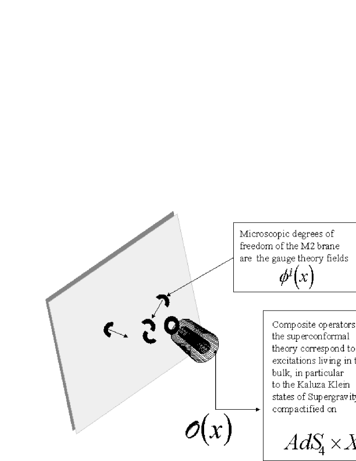
Figure 6: Conformal superfields are composite operators in the gauge theory

can be identified with the components of the conformal superfields described in the previous section and matching the Kaluza Klein classical spectrum.

According to the specific horizon $X^{7}$, the world volume gauge group is of the form:

$$G^{WV}_{gauge}=U(k_{1}\,N)^{\ell_{1}}\,\times\,\dots\,\times\,U(k_{n}N)^{\ell_{n}}$$ (5.2)

where $k_{i}$ and $\ell_{i}$ are integer number and where the correspondence is true in the large $N\to\infty$ limit. Indeed $N$ is to be identified with the number of $M2$ branes in the stack.

In addition the gauge theory has a flavor group which coincides with the gauge group of Kaluza Klein supergravity, namely with the isometry group of the $X^{7}$ horizon:

$$G^{WV}_{flavor}=G_{KK}^{bulk}=\mbox{isometry}(X^{7})$$ (5.3)

Since our goal is to study the general features of the $AdS_{4}/CFT_{3}$ correspondence, rather than specific cases, we concentrate on the construction of a generic ${\cal N}=2$ gauge theory with an arbitrary gauge group and an arbitrary number of chiral multiplets in generic interaction. We are mostly interested in the final formulae for the scalar potential and on the restrictions that guarantee an enlargement of supersymmetry to ${\cal N}=4$ or ${\cal N}=8$, but we provide a complete construction of the lagrangian and of the supersymmetry transformation rules. To this effect we utilize the time honored method of rheonomy [44, 45, 46] that yields the the result for the lagrangian and the supersymmetry rules in component form avoiding the too much implicit notation of superfield formulation. The first step in the rheonomic construction of a rigid supersymmetric theory involves writing the structural equations of rigid superspace.

5.1 ${\cal N}=2,\,d=3$ rigid superspace

The $d\!\!=\!\!3,~{}{\cal N}$–extended superspace is viewed as the supercoset space:

$${\cal M}^{\cal N}_{3}=\frac{ISO(1,2|{\cal N})}{SO(1,2)}\,\equiv\,\frac{Z\left[ISO(1,2|{\cal N})\right]}{SO(1,2)\times{\rm I\kern-1.79993ptR}^{{\cal N}({\cal N}-1)/2}}$$ (5.4)

where $ISO(1,2|{\cal N})$ is the ${\cal N}$–extended Poincaré superalgebra in three–dimensions. It is the subalgebra of $Osp({\cal N}|4)$ (see eq. (2.31)) spanned by the generators $J_{m}$, $P_{m}$, $q^{i}$. The central extension $Z\left[ISO(1,2|{\cal N})\right]$ which is not contained in $Osp({\cal N}|4)$ is obtained by adjoining to $ISO(1,2|{\cal N})$ the central charges that generate the subalgebra ${\rm I\kern-1.79993ptR}^{{\cal N}({\cal N}-1)/2}$. Specializing our analysis to the case ${\cal N}\!\!=\!\!2$, we can define the new generators:

$$\left\{\begin{array}[]{ccl}Q&=&\sqrt{2}q^{-}=(q^{1}-iq^{2})\\ Q^{c}&=&\sqrt{2}iq^{+}=i(q^{1}+iq^{2})\\ Z&=&Z^{12}\end{array}\right.$$ (5.5)

The left invariant one–form $\Omega$ on ${\cal M}^{\cal N}_{3}$ is:

$$\Omega=iV^{m}P_{m}-i\omega^{mn}J_{mn}+i\overline{\psi^{c}}Q-i\overline{\psi}Q^{c}+i{\cal B}Z\,.$$ (5.6)

The superalgebra (2.31) defines all the structure constants apart from those relative to the central charge that are trivially determined. Hence we can write:

$$d\Omega-\Omega\wedge\Omega = \left(dV^{m}-\omega^{m}_{\ n}\wedge V^{n}+i\overline{\psi}\wedge\gamma^{m}\psi+i\overline{\psi}^{c}\wedge\gamma^{m}\psi^{c}\right)P_{m}$$ (5.7)

$$-{\textstyle\frac{1}{2}}i\left(d\omega^{mn}-\omega^{m}_{\ p}\wedge\omega^{pn}\right)J_{mn}$$

$$+\left(d\overline{\psi}^{c}+{\textstyle\frac{1}{2}}\omega^{mn}\wedge\overline{\psi}^{c}\gamma_{mn}\right)Q$$

$$+\left(d\overline{\psi}-{\textstyle\frac{1}{2}}\omega^{mn}\wedge\overline{\psi}\gamma_{mn}\right)Q^{c}$$

$$+i\left(d{\cal B}+i\overline{\psi}^{c}\wedge\psi^{c}-i\overline{\psi}\wedge\psi\right)Z$$

Imposing the Maurer-Cartan equation $d\Omega-\Omega\wedge\Omega=0$ is equivalent to imposing flatness in superspace, i.e. global supersymmetry. So we have

$$\left\{\begin{array}[]{ccl}dV^{m}-\omega^{m}_{\ n}\wedge V^{n}&=&-i\overline{\psi}^{c}\wedge\gamma^{m}\psi^{c}-i\overline{\psi}\wedge\gamma^{m}\psi\\ d\omega^{mn}&=&\omega^{m}_{\ p}\wedge\omega^{pn}\\ d\overline{\psi}^{c}&=&-{\textstyle\frac{1}{2}}\omega^{mn}\wedge\overline{\psi}^{c}\gamma_{mn}\\ d\overline{\psi}&=&{\textstyle\frac{1}{2}}\omega^{mn}\wedge\overline{\psi}\gamma_{mn}\\ d{\cal B}&=&-i\overline{\psi}^{c}\wedge\psi^{c}+i\overline{\psi}\wedge\psi\end{array}\right.$$ (5.8)

The simplest solution for the supervielbein and connection is:

$$\left\{\begin{array}[]{ccl}V^{m}&=&dx^{m}-i\overline{\theta}^{c}\gamma^{m}d\theta^{c}-i\overline{\theta}\gamma^{m}d\theta\\ \omega^{mn}&=&0\\ \psi&=&d\theta\\ \psi^{c}&=&d\theta^{c}\\ {\cal B}&=&-i\overline{\theta}^{c}\,d\theta^{c}+i\overline{\theta}\,d\theta\end{array}\right.$$

The superderivatives discussed in the previous sections (compare with (4.4)),

$$\left\{\begin{array}[]{ccl}D_{m}&=&\partial_{m}\\ D&=&\frac{\partial}{\partial\overline{\theta}}-i\gamma^{m}\theta\partial_{m}\\ D^{c}&=&\frac{\partial}{\partial\overline{\theta}^{c}}-i\gamma^{m}\theta^{c}\partial_{m}\\ \end{array}\right.,$$ (5.9)

are the vectors dual to these one–forms.

5.2 Rheonomic construction of the ${\cal N}=2,~{}d=3,$ lagrangian

As stated we are interested in the generic form of ${\cal N}=2,~{}d=3$ super Yang Mills theory coupled to $n$ chiral multiplets arranged into a generic representation $\cal R$ of the gauge group $\cal G$.

In ${\cal N}=2,~{}d=3$ supersymmetric theories, two formulations are allowed: the on–shell and the off–shell one. In the on–shell formulation which contains only the physical fields, the supersymmetry transformations rules close the supersymmetry algebra only upon use of the field equations. On the other hand the off–shell formulation contains further auxiliary, non dynamical fields that make it possible for the supersymmetry transformations rules to close the supersymmetry algebra identically. By solving the field equations of the auxiliary fields these latter can be eliminated and the on–shell formulation can be retrieved. We adopt the off–shell formulation.

5.2.1 The gauge multiplet

The three–dimensional ${\cal N}=2$ vector multiplet contains the following Lie-algebra valued fields:

$$\left({\cal A},\lambda,\lambda^{c},M,P\right)\,,$$ (5.10)

where ${\cal A}={\cal A}^{I}t_{I}$ is the real gauge connection one–form, $\lambda$ and $\lambda^{c}$ are two complex Dirac spinors (the gauginos), $M$ and $P$ are real scalars; $P$ is an auxiliary field.

The field strength is:

$$F=d{\cal A}+i{\cal A}\wedge{\cal A}\,.$$ (5.11)

The covariant derivative on the other fields of the gauge multiplets is defined as:

$$\nabla X=dX+i\left[{\cal A},X\right]\,.$$ (5.12)

From (5.11) and (5.12) we obtain the Bianchi identity:

$$\nabla^{2}X=i\left[F,X\right]\,.$$ (5.13)

The rheonomic parametrization of the curvatures is given by:

$$\left\{\begin{array}[]{ccl}F&=&F_{mn}V^{m}V^{n}-i\overline{\psi}^{c}\gamma_{m}\lambda V^{m}-i\overline{\psi}\gamma_{m}\lambda^{c}V^{m}+iM\left(\overline{\psi}\psi-\overline{\psi}^{c}\psi^{c}\right)\\ \nabla\lambda&=&V^{m}\nabla_{m}\lambda+\nabla\!\!\!\!/M\psi^{c}-F_{mn}\gamma^{mn}\psi^{c}+iP\psi^{c}\\ \nabla\lambda^{c}&=&V^{m}\nabla_{m}\lambda^{c}-\nabla\!\!\!\!/M\psi-F_{mn}\gamma^{mn}\psi-iP\psi\\ \nabla M&=&V^{m}\nabla_{m}M+i\overline{\psi}\lambda^{c}-i\overline{\psi}^{c}\lambda\\ \nabla P&=&V^{m}\nabla_{m}P+\overline{\psi}\nabla\!\!\!\!/\lambda^{c}-\overline{\psi}^{c}\nabla\!\!\!\!/\lambda-i\overline{\psi}\left[\lambda^{c},M\right]-i\overline{\psi}^{c}\left[\lambda,M\right]\end{array}\right.$$ (5.14)

and we also have:

$$\left\{\begin{array}[]{ccl}\nabla F_{mn}&=&V^{p}\nabla_{p}F_{mn}+i\overline{\psi}^{c}\gamma_{[m}\nabla_{n]}\lambda+i\overline{\psi}\gamma_{[m}\nabla_{n]}\lambda^{c}\\ \nabla\nabla_{m}M&=&V^{n}\nabla_{n}\nabla_{m}M+i\overline{\psi}\nabla_{m}\lambda^{c}-i\overline{\psi}^{c}\nabla_{m}\lambda+\overline{\psi}^{c}\gamma_{m}\left[\lambda,M\right]+\overline{\psi}\gamma_{m}\left[\lambda^{c},M\right]\\ \nabla\nabla_{m}\lambda&=&V^{n}\nabla_{n}\nabla_{m}\lambda+\nabla_{m}\nabla_{n}M\gamma^{n}\psi^{c}-\nabla_{m}F_{np}\gamma^{np}\psi^{c}\\ &&+i\nabla_{m}P\psi^{c}+\overline{\psi}\gamma_{m}\left[\lambda^{c},\lambda\right]\\ \nabla_{[p}F_{mn]}&=&0\\ \nabla_{[m}\nabla_{n]}M&=&i\left[F_{mn},M\right]\\ \nabla_{[m}\nabla_{n]}\lambda&=&i\left[F_{mn},\lambda\right]\end{array}\right.$$ (5.15)

The off–shell formulation of the theory contains an arbitrariness in the choice of the functional dependence of the auxiliary fields on the physical fields. Consistency with the Bianchi identities forces the generic expression of $P$ as a function of $M$ to be:

$$P^{I}=2\alpha M^{I}+\zeta^{\widetilde{I}}{\cal C}_{\widetilde{I}}^{\ I}\,,$$ (5.16)

where $\alpha,~{}\zeta^{\widetilde{I}}$ are arbitrary real parameters and ${\cal C}_{\widetilde{I}}^{\ I}$ is the projector on the center of $Z[\cal G]$ of the gauge Lie algebra. The terms in the lagrangian proportional to $\alpha$ and $\zeta$ are separately supersymmetric. In the bosonic lagrangian, the part proportional to $\alpha$ is a Chern Simons term, while the part proportional to $\zeta$ constitutes the Fayet Iliopoulos term. Note that the Fayet Iliopoulos terms are associated only with a central abelian subalgebra of the gauge algebra $\cal G$.

Enforcing (5.16) we get the following equations of motion for the spinors:

$$\left\{\begin{array}[]{c}\nabla\!\!\!\!/\lambda=2i\alpha\lambda-i\left[\lambda,M\right]\\ \\ \nabla\!\!\!\!/\lambda^{c}=2i\alpha\lambda^{c}+i\left[\lambda^{c},M\right]\end{array}\right.$$ (5.17)

Taking the covariant derivatives of these, we obtain the equations of motion for the bosonic fields:

$$\left\{\begin{array}[]{c}\nabla_{m}\nabla^{m}M^{I}=-4\alpha^{2}M^{I}-2\alpha\zeta^{\widetilde{I}}{\cal C}_{\widetilde{I}}^{\ I}-2\left[\overline{\lambda},\lambda\right]^{I}\\ \nabla^{n}F_{mn}=-\alpha\epsilon_{mnp}F^{np}-{\textstyle\frac{i}{2}}\left[\nabla_{m}M,M\right]\end{array}\right.$$ (5.18)

Using the rheonomic approach we find the following superspace lagrangian for the gauge multiplet:

$${\cal L}_{gauge}={\cal L}_{gauge}^{Maxwell}+{\cal L}_{gauge}^{Chern-Simons}+{\cal L}_{gauge}^{Fayet-Iliopoulos}\,,$$ (5.19)

where

$${\cal L}_{gauge}^{Maxwell} = Tr\left\{-F^{mn}\left[F+i\overline{\psi}^{c}\gamma_{m}\lambda V^{m}+i\overline{\psi}\gamma_{m}\lambda^{c}V^{m}-2iM\overline{\psi}\psi\right]V^{p}\epsilon_{mnp}\right.$$ (5.20)

$$+ {\textstyle\frac{1}{6}}F_{qr}F^{qr}V^{m}V^{n}V^{p}\epsilon_{mnp}-{\textstyle\frac{1}{4}}i\epsilon_{mnp}\left[\nabla\overline{\lambda}\gamma^{m}\lambda+\nabla\overline{\lambda}^{c}\gamma^{m}\lambda^{c}\right]V^{n}V^{p}$$

$$+ {\textstyle\frac{1}{2}}\epsilon_{mnp}{\cal M}^{m}\left[\nabla M-i\overline{\psi}\lambda^{c}+i\overline{\psi}^{c}\lambda\right]V^{n}V^{p}-{\textstyle\frac{1}{12}}{\cal M}^{d}{\cal M}_{d}\epsilon_{mnp}V^{m}V^{n}V^{p}$$

$$+ \nabla M\overline{\psi}^{c}\gamma_{c}\lambda V^{p}-\nabla M\overline{\psi}\gamma_{p}\lambda^{c}V^{p}$$

$$+ F\overline{\psi}^{c}\lambda+F\overline{\psi}\lambda^{c}+{\textstyle\frac{1}{2}}i\overline{\lambda}^{c}\lambda\overline{\psi}^{c}\gamma_{m}\psi V^{m}+{\textstyle\frac{1}{2}}i\overline{\lambda}\lambda^{c}\overline{\psi}\gamma_{m}\psi^{c}V^{m}$$

$$+ {\textstyle\frac{1}{12}}{\cal P}^{2}V^{m}V^{n}V^{p}\epsilon_{mnp}-2i(\overline{\psi}\psi)M\left[\overline{\psi}^{c}\lambda+\overline{\psi}\lambda^{c}\right]$$

$$- \left.{\textstyle\frac{1}{6}}M\left[\overline{\lambda},\lambda\right]V^{m}V^{n}V^{p}\epsilon_{mnp}\right\}\,,$$

$${\cal L}_{gauge}^{Chern-Simons} = \alpha Tr\left\{-\left(A\wedge F-iA\wedge A\wedge A\right)-{\textstyle\frac{1}{3}}MP\epsilon_{mnp}V^{m}V^{n}V^{p}\right.$$ (5.21)

$$+ {\textstyle\frac{1}{3}}\overline{\lambda}\lambda\epsilon_{mnp}V^{m}V^{n}V^{p}+M\epsilon_{mnp}\left[\overline{\psi}^{c}\gamma^{m}\lambda-\overline{\psi}\gamma^{m}\lambda^{c}\right]V^{n}V^{p}$$

$$\left.-2iM^{2}\overline{\psi}\gamma_{m}\psi V^{m}\right\}$$

$${\cal L}_{gauge}^{Fayet-Iliopoulos} = Tr\left\{\zeta{\cal C}\left[-{\textstyle\frac{1}{6}}P\epsilon_{mnp}V^{m}V^{n}V^{p}+{\textstyle\frac{1}{2}}\epsilon_{mnp}\left(\overline{\psi}^{c}\gamma^{m}\lambda-\overline{\psi}\gamma^{m}\lambda^{c}\right)V^{n}V^{p}\right.\right.$$ (5.22)

$$\left.\left.-2iM\overline{\psi}\gamma_{m}\psi V^{m}-2i{\cal A}\overline{\psi}\psi\right]\right\}$$

5.2.2 Chiral multiplet

The chiral multiplet contains the following fields:

$$\left(z^{i},\chi^{i},H^{i}\right)$$ (5.23)

where $z^{i}$ are complex scalar fields which parametrize a Kähler manifold. Since we are interested in microscopic theories with canonical kinetic terms we take this Kähler manifold to be flat and we choose its metric to be the constant $\eta_{ij^{*}}\equiv\mbox{diag}(+,+,\dots,+)$. The other fields in the chiral multiplet are $\chi^{i}$ which is a two components Dirac spinor and $H^{i}$ which is a complex scalar auxiliary field. The index $i$ runs in the representation $\cal R$ of $\cal G$.

The covariant derivative of the fields $X^{i}$ in the chiral multiplet is:

$$\nabla X^{i}=dX^{i}+i\eta^{ii^{*}}{\cal A}^{I}(T_{I})_{i^{*}j}X^{j}\,,$$ (5.24)

where $(T_{I})_{i^{*}j}$ are the hermitian generators of $\cal G$ in the representation $\cal R$. The covariant derivative of the complex conjugate fields $\overline{X}^{i^{*}}$ is:

$$\nabla\overline{X}^{i^{*}}=d\overline{X}^{i^{*}}-i\eta^{i^{*}i}{\cal A}^{I}(\overline{T}_{I})_{ij^{*}}\overline{X}^{j^{*}}\,,$$ (5.25)

where

$$(\overline{T}_{I})_{ij^{*}}\equiv\overline{(T_{I})_{i^{*}j}}=(T_{I})_{j^{*}i}\,.$$ (5.26)

The rheonomic parametrization of the curvatures is given by:

$$\left\{\begin{array}[]{ccl}\nabla z^{i}&=&V^{m}\nabla_{m}z^{i}+2\overline{\psi}^{c}\chi^{i}\\ \nabla\chi^{i}&=&V^{m}\nabla_{m}\chi^{i}-i\nabla\!\!\!\!/z^{i}\psi^{c}+H^{i}\psi-M^{I}(T_{I})^{i}_{\,j}z^{j}\psi^{c}\\ \nabla H^{i}&=&V^{m}\nabla_{m}H^{i}-2i\overline{\psi}\nabla\!\!\!\!/\chi^{i}-2i\overline{\psi}\lambda^{I}(T_{I})^{i}_{\,j}z^{j}+2M^{I}(T_{I})^{i}_{\,j}\overline{\psi}\chi^{j}\end{array}\right.\,.$$ (5.27)

We can choose the auxiliary fields $H^{i}$ to be the derivatives of an arbitrary antiholomorphic superpotential $\overline{W}(\overline{z})$:

$$H^{i}=\eta^{ij^{*}}\frac{\partial\overline{W}(\overline{z})}{\partial z^{j^{*}}}=\eta^{ij^{*}}\partial_{j^{*}}\overline{W}$$ (5.28)

Enforcing eq. (5.28) we get the following equations of motion for the spinors:

$$\left\{\begin{array}[]{c}\nabla\!\!\!\!/\chi^{i}=i\eta^{ij^{*}}\partial_{j^{*}}\partial_{k^{*}}\overline{W}\chi^{ck^{*}}-\lambda^{I}(T_{I})^{i}_{\,j}z^{j}-iM^{I}(T_{I})^{i}_{\,j}\chi^{j}\\ \\ \nabla\!\!\!\!/\chi^{ci^{*}}=i\eta^{i^{*}j}\partial_{j}\partial_{k}W\chi^{k}+\lambda^{cI}(\overline{T}_{I})^{i^{*}}_{\,j^{*}}\overline{z}^{j^{*}}-iM^{I}(\overline{T}_{I})^{i^{*}}_{\,j^{*}}\chi^{cj^{*}}\end{array}\right.\,.$$ (5.29)

Taking the differential of (5.29) one obtains the equation of motion for $z$:

$$\Box z^{i} = \eta^{ii^{*}}\partial_{i^{*}}\partial_{j^{*}}\partial_{k^{*}}\overline{W}(\overline{z})\left(\overline{\chi}^{j^{*}}\chi^{ck^{*}}\right)-\eta^{ij^{*}}\partial_{j^{*}}\partial_{k^{*}}\overline{W}(\overline{z})\partial_{i}W(z)$$ (5.30)

$$+P^{I}(T_{I})^{i}_{\,j}z^{j}-M^{I}M^{J}(T_{I}T_{J})^{i}_{\,j}z^{j}-2i\overline{\lambda}^{I}(T_{I})^{i}_{\,j}\chi^{j}$$

The first order Lagrangian for the chiral multiplet (5.23) is:

$${\cal L}_{chiral}={\cal L}_{chiral}^{Wess-Zumino}+{\cal L}_{chiral}^{superpotential}\,,$$ (5.31)

where

$${\cal L}_{chiral}^{Wess-Zumino} = {\textstyle\frac{1}{2}}\epsilon_{mnp}\overline{\Pi}^{m\,i^{*}}\eta_{i^{*}j}\left[\nabla z^{j}-2\overline{\psi}^{c}\chi^{j}\right]V^{n}V^{p}$$ (5.32)

$$+ {\textstyle\frac{1}{2}}\epsilon_{mnp}\Pi^{m\,i}\eta_{ij^{*}}\left[\nabla\overline{z}^{j^{*}}-2\overline{\chi}\psi^{c\,j^{*}}\right]V^{n}V^{p}$$

$$- {\textstyle\frac{1}{6}}\epsilon_{mnp}\eta_{ij^{*}}\Pi_{q}^{\,i}\overline{\Pi}^{q\,j^{*}}V^{m}V^{n}V^{p}$$

$$+ {\textstyle\frac{1}{2}}i\epsilon_{mnp}\eta_{ij^{*}}\left[\overline{\chi}^{j^{*}}\gamma^{m}\nabla\chi^{i}+\overline{\chi}^{c\,i}\gamma^{m}\nabla\chi^{c\,j^{*}}\right]V^{n}V^{p}$$

$$+ 2i\eta_{ij^{*}}\left[\nabla z^{i}\overline{\psi}\gamma_{m}\chi^{c\,j^{*}}-\nabla\overline{z}^{j^{*}}\overline{\chi}^{c\,i}\gamma_{m}\psi\right]V^{m}$$

$$- 2i\eta_{ij^{*}}\left(\overline{\chi}^{j^{*}}\gamma_{m}\chi^{i}\right)\left(\overline{\psi}^{c}\psi^{c}\right)V^{m}-2i\eta_{ij^{*}}\left(\overline{\chi}^{j^{*}}\chi^{i}\right)\left(\overline{\psi}^{c}\gamma_{m}\psi^{c}\right)V^{m}$$

$$+ {\textstyle\frac{1}{6}}\eta_{ij^{*}}H^{i}\overline{H}^{j^{*}}\epsilon_{mnp}V^{m}V^{n}V^{p}+\left(\overline{\psi}\psi\right)\eta_{ij^{*}}\left[\overline{z}^{j^{*}}\nabla z^{i}-z^{i}\nabla\overline{z}^{j^{*}}\right]$$

$$+ i\epsilon_{mnp}z^{i}M^{I}(T_{I})_{ij^{*}}\overline{\chi}^{j^{*}}\gamma^{m}\psi^{c}V^{n}V^{p}$$

$$+ i\epsilon_{mnp}\overline{z}^{j^{*}}M^{I}(T_{I})_{j^{*}i}\overline{\chi}^{c\,i}\gamma^{m}\psi V^{n}V^{p}$$

$$- {\textstyle\frac{1}{3}}M^{I}(T_{I})_{ij^{*}}\overline{\chi}^{j^{*}}\chi^{i}\epsilon_{mnp}V^{m}V^{n}V^{p}$$

$$+ {\textstyle\frac{1}{3}}i\left[\overline{\chi}^{j^{*}}\lambda^{I}(T_{I})_{j^{*}i}z^{i}-\overline{\chi}^{c\,i}\lambda^{c\,I}(T_{I})_{ij^{*}}\overline{z}^{j^{*}}\right]\epsilon_{mnp}V^{m}V^{n}V^{p}$$

$$+ {\textstyle\frac{1}{6}}z^{i}P^{I}(T_{I})_{ij^{*}}\overline{z}^{j^{*}}\epsilon_{mnp}V^{m}V^{n}V^{p}$$

$$- {\textstyle\frac{1}{2}}\left(\overline{\psi}^{c}\gamma^{m}\lambda^{I}(T_{I})_{ij^{*}}\right)z^{i}\overline{z}^{j^{*}}\epsilon_{mnp}V^{n}V^{p}$$

$$+ {\textstyle\frac{1}{2}}\left(\overline{\psi}\gamma^{m}\lambda^{c\,I}(T_{I})_{ij^{*}}\right)z^{i}\overline{z}^{j^{*}}\epsilon_{mnp}V^{n}V^{p}$$

$$- {\textstyle\frac{1}{6}}M^{I}M^{J}\,z^{i}(T_{I}T_{J})_{ij^{*}}\overline{z}^{j^{*}}\epsilon_{mnp}V^{m}V^{n}V^{p}$$

$$+ 2iM^{I}(T_{I})_{ij^{*}}z^{i}\overline{z}^{j^{*}}\overline{\psi}\gamma_{m}\psi V^{m}\,,$$

and

$${\cal L}_{chiral}^{superpotential} = -i\epsilon_{mnp}\left[\overline{\chi}^{j^{*}}\gamma^{m}\partial_{j^{*}}\overline{W}(\overline{z})\psi+\overline{\chi}^{c\,j}\gamma^{m}\partial_{j}\overline{W}(z)\psi^{c}\right]V^{n}V^{p}$$ (5.33)

$$+ {\textstyle\frac{1}{6}}\left[\partial_{i}\partial_{j}W(z)\overline{\chi}^{c\,i}\chi^{j}+\partial_{i^{*}}\partial_{j^{*}}\overline{W}(\overline{z})\overline{\chi}^{i^{*}}\chi^{c\,j^{*}}\right]\epsilon_{mnp}V^{m}V^{n}V^{p}$$

$$- {\textstyle\frac{1}{6}}\left[H^{i}\partial_{i}W(z)+\overline{H}^{j^{*}}\partial_{j^{*}}\overline{W}(\overline{z})\right]\epsilon_{mnp}V^{m}V^{n}V^{p}$$

$$- 2i\left[W(z)+\overline{W}(\overline{z})\right]\overline{\psi}\gamma_{m}\psi^{c}V^{m}$$

5.2.3 The space–time Lagrangian

In the rheonomic approach ([44]), the total three–dimensional ${\cal N}\!\!=\!\!2$ lagrangian:

$${\cal L}^{{\cal N}=2}={\cal L}_{gauge}+{\cal L}_{chiral}$$ (5.34)

is a closed ($d{\cal L}^{{\cal N}=2}=0$) three–form defined in superspace. The action is given by the integral of ${\cal L}^{{\cal N}=2}$ on a generic bosonic three–dimensional surface ${\cal M}_{3}$ in superspace:

$$S=\int_{{\cal M}_{3}}{\cal L}^{{\cal N}=2}\,.$$ (5.35)

Supersymmetry transformations can be viewed as global translations in superspace which move ${\cal M}_{3}$. Then, being ${\cal L}^{{\cal N}=2}$ closed, the action is invariant under global supersymmetry transformations.

We choose as bosonic surface the one defined by:

$$\theta=d\theta=0\,.$$ (5.36)

Then the space–time lagrangian, i.e. the pull–back of ${\cal L}^{{\cal N}=2}$ on ${\cal M}_{3}$, is:

$${\cal L}^{{\cal N}=2}_{st}={\cal L}^{kinetic}_{st}+{\cal L}^{fermion~{}mass}_{st}+{\cal L}^{potential}_{st}\,,$$ (5.37)

where

$${\cal L}_{st}^{kinetic} = \left\{\eta_{ij^{*}}\nabla_{m}z^{i}\nabla^{m}\overline{z}^{j^{*}}+i\eta_{ij^{*}}\left(\overline{\chi}^{j^{*}}\nabla\!\!\!\!/\chi^{i}+\overline{\chi}^{c\,i}\nabla\!\!\!\!/\chi^{c\,j^{*}}\right)\right.$$ (5.38)

$$-g_{IJ}F^{I}_{mn}F^{J\,mn}+{\textstyle\frac{1}{2}}g_{IJ}\nabla_{m}M^{I}\nabla^{m}M^{J}$$

$$+\left.{\textstyle\frac{1}{2}}ig_{IJ}\left(\overline{\lambda}^{I}\nabla\!\!\!\!/\lambda^{J}+\overline{\lambda}^{c\,I}\nabla\!\!\!\!/\lambda^{c\,J}\right)\right\}d^{3}x$$

$${\cal L}_{st}^{fermion~{}mass} = \left\{i\left(\overline{\chi}^{c\,i}\partial_{i}\partial_{j}W(z)\chi^{j}+\overline{\chi}^{i^{*}}\partial_{i^{*}}\partial_{j^{*}}\overline{W}(\overline{z})\chi^{c\,j^{*}}\right)\right.$$ (5.39)

$$-f_{IJK}M^{I}\overline{\lambda}^{J}\lambda^{K}-2\overline{\chi}^{i^{*}}M^{I}(T_{I})_{ij^{*}}\chi^{j^{*}}$$

$$+2i\left(\overline{\chi}^{i^{*}}\lambda^{I}(T_{I})_{i^{*}j}z^{j}-\overline{\chi}^{c\,i}\lambda^{I}(T_{I})_{ij^{*}}\overline{z}^{j^{*}}\right)$$

$$\left.+2\alpha g_{IJ}\overline{\lambda}^{I}\lambda^{J}\right\}d^{3}x$$

$${\cal L}_{st}^{potential} = -U(z,\overline{z},H,\overline{H},M,P)d^{3}x\,,$$ (5.40)

and

$$U(z,\overline{z},H,\overline{H},M,P) = H^{i}\partial_{i}W(z)+\overline{H}^{j^{*}}\partial_{j^{*}}\overline{W}(\overline{z})-\eta_{ij^{*}}H^{i}\overline{H}^{j^{*}}$$ (5.41)

$$-{\textstyle\frac{1}{2}}g_{IJ}P^{I}P^{J}-z^{i}P^{I}(T_{I})_{ij^{*}}\overline{z}^{j^{*}}$$

$$+z^{i}M^{I}(T_{I})_{ij^{*}}\eta^{j^{*}k}M^{J}(T_{J})_{kl^{*}}\overline{z}^{l^{*}}$$

$$+2\alpha g_{IJ}M^{I}P^{J}+\zeta^{\widetilde{I}}{\cal C}_{\widetilde{I}}^{\ I}g_{IJ}P^{J}$$

From the variation of the lagrangian with respect to the auxiliary fields $H^{i}$ and $P^{I}$ we find:

$$H^{i} = \eta^{ij^{*}}\partial_{j^{*}}\overline{W}(\overline{z})\,,$$ (5.42)

$$P^{I} = D^{I}(z,\overline{z})+2\alpha M^{I}+\zeta^{\widetilde{I}}{\cal C}_{\widetilde{I}}^{\ I}\,,$$ (5.43)

where

$$D^{I}(z,\overline{z})=-\overline{z}^{i^{*}}(T_{I})_{i^{*}j}z^{j}$$ (5.44)

Substituting this expressions in the potential (5.41) we obtain:

$$U(z,\overline{z},M) = -\partial_{i}W(z)\eta^{ij^{*}}\partial_{j^{*}}\overline{W}(\overline{z})$$ (5.45)

$$+{\textstyle\frac{1}{2}}g^{IJ}\left(\overline{z}^{i^{*}}(T_{I})_{i^{*}j}z^{j}\right)\left(\overline{z}^{k^{*}}(T_{J})_{k^{*}l}z^{l}\right)$$

$$+\overline{z}^{i^{*}}M^{I}(T_{I})_{i^{*}j}\eta^{jk^{*}}M^{J}(T_{J})_{k^{*}l}z^{l}$$

$$-2\alpha^{2}g_{IJ}M^{I}M^{J}-2\alpha\zeta^{\widetilde{I}}{\cal C}_{\widetilde{I}}^{\ I}g_{IJ}M^{J}-{\textstyle\frac{1}{2}}\zeta^{\widetilde{I}}{\cal C}_{\widetilde{I}}^{\ I}g_{IJ}\zeta^{\widetilde{J}}{\cal C}_{\widetilde{J}}^{\ J}$$

$$-2\alpha M^{I}\left(\overline{z}^{i^{*}}(T_{I})_{i^{*}j}z^{j}\right)-\zeta^{\widetilde{I}}{\cal C}_{\widetilde{I}}^{\ I}\left(\overline{z}^{i^{*}}(T_{I})_{i^{*}j}z^{j}\right)$$

5.3 A particular ${\cal N}=2$ theory: ${\cal N}=4$

A general lagrangian for matter coupled rigid ${\cal N}=4,d=3$ super Yang Mills theory is easily obtained from the dimensional reduction of the ${\cal N}=2,d=4$ gauge theory (see [58]). The bosonic sector of this latter lagrangian is the following:

$${\cal L}_{bosonic}^{{\cal N}=4} = -\frac{1}{g^{2}_{{}_{YM}}}g_{IJ}F^{I}_{mn}F^{J\,mn}+\frac{1}{2g^{2}_{{}_{YM}}}g_{IJ}\nabla_{m}M^{I}\nabla^{m}M^{J}$$ (5.46)

$$+\frac{2}{g^{2}_{{}_{YM}}}g_{IJ}\nabla_{m}\overline{Y}^{I}\nabla^{m}Y^{J}+\frac{1}{2}Tr\left(\nabla_{m}\overline{\bf Q}\nabla^{m}{\bf Q}\right)$$

$$-\frac{1}{g^{2}_{{}_{YM}}}g_{IN}f^{I}_{JK}f^{N}_{LM}\,M^{J}\overline{Y}^{K}\,M^{L}Y^{M}-M^{I}M^{J}Tr\left(\overline{\bf Q}(\hat{T}_{I}\,\hat{T}_{J}){\bf Q}\right)$$

$$-\frac{2}{g^{2}_{{}_{YM}}}g_{IN}f^{I}_{JK}f^{N}_{LM}\,\overline{Y}^{J}Y^{K}\,\overline{Y}^{L}Y^{M}-\overline{Y}^{I}Y^{J}\,Tr\left(\overline{\bf Q}\left\{\hat{T}_{I},\hat{T}_{J}\right\}{\bf Q}\right)$$

$$-\frac{1}{4}g^{2}_{{}_{YM}}g_{IJ}Tr\left(\overline{\bf Q}(\hat{T}^{I}){\bf Q}\,\overline{\bf Q}(\hat{T}^{J}){\bf Q}\right)$$

The bosonic matter field content is given by two kinds of fields. First we have a complex field $Y^{I}$ in the adjoint representation of the gauge group, which belongs to a chiral multiplet. Secondly, we have an $n$-uplet of quaternions ${\bf Q}$, which parametrize a (flat) HyperKähler manifold:

$${\bf Q}=\left(\begin{array}[]{ccl}Q^{1}&=&q^{1|0}\mathord{\!\leavevmode\hbox{ \begin{picture}(0.6,0.7)\put(0.0,0.0){\line(1,0){0.5}} \put(0.15,0.0){\line(0,1){0.7}} \put(0.35,0.0){\line(0,1){0.8}} \put(0.3,0.8){\rule{0.5pt}{0.5pt}}\put(0.26,0.78){\rule{0.5pt}{0.5pt}}\put(0.22,0.76){\rule{0.5pt}{0.5pt}}\put(0.18,0.74){\rule{0.5pt}{0.5pt}}\put(0.14,0.72){\rule{0.5pt}{0.5pt}}\put(0.1,0.7){\rule{0.5pt}{0.5pt}}\put(0.06,0.68){\rule{0.5pt}{0.5pt}}\put(0.02,0.66){\rule{0.5pt}{0.5pt}}\put(-0.02,0.64){\rule{0.5pt}{0.5pt}}\put(-0.06,0.62){\rule{0.5pt}{0.5pt}} \end{picture}}}-iq^{1|x}\sigma_{x}\\ Q^{2}&=&q^{2|0}\mathord{\!\leavevmode\hbox{ \begin{picture}(0.6,0.7)\put(0.0,0.0){\line(1,0){0.5}} \put(0.15,0.0){\line(0,1){0.7}} \put(0.35,0.0){\line(0,1){0.8}} \put(0.3,0.8){\rule{0.5pt}{0.5pt}}\put(0.26,0.78){\rule{0.5pt}{0.5pt}}\put(0.22,0.76){\rule{0.5pt}{0.5pt}}\put(0.18,0.74){\rule{0.5pt}{0.5pt}}\put(0.14,0.72){\rule{0.5pt}{0.5pt}}\put(0.1,0.7){\rule{0.5pt}{0.5pt}}\put(0.06,0.68){\rule{0.5pt}{0.5pt}}\put(0.02,0.66){\rule{0.5pt}{0.5pt}}\put(-0.02,0.64){\rule{0.5pt}{0.5pt}}\put(-0.06,0.62){\rule{0.5pt}{0.5pt}} \end{picture}}}-iq^{2|x}\sigma_{x}\\ &\cdots&\\ Q^{A}&=&q^{A|0}\mathord{\!\leavevmode\hbox{ \begin{picture}(0.6,0.7)\put(0.0,0.0){\line(1,0){0.5}} \put(0.15,0.0){\line(0,1){0.7}} \put(0.35,0.0){\line(0,1){0.8}} \put(0.3,0.8){\rule{0.5pt}{0.5pt}}\put(0.26,0.78){\rule{0.5pt}{0.5pt}}\put(0.22,0.76){\rule{0.5pt}{0.5pt}}\put(0.18,0.74){\rule{0.5pt}{0.5pt}}\put(0.14,0.72){\rule{0.5pt}{0.5pt}}\put(0.1,0.7){\rule{0.5pt}{0.5pt}}\put(0.06,0.68){\rule{0.5pt}{0.5pt}}\put(0.02,0.66){\rule{0.5pt}{0.5pt}}\put(-0.02,0.64){\rule{0.5pt}{0.5pt}}\put(-0.06,0.62){\rule{0.5pt}{0.5pt}} \end{picture}}}-iq^{A|x}\sigma_{x}\\ &\cdots&\\ Q^{n}&=&q^{n|0}\mathord{\!\leavevmode\hbox{ \begin{picture}(0.6,0.7)\put(0.0,0.0){\line(1,0){0.5}} \put(0.15,0.0){\line(0,1){0.7}} \put(0.35,0.0){\line(0,1){0.8}} \put(0.3,0.8){\rule{0.5pt}{0.5pt}}\put(0.26,0.78){\rule{0.5pt}{0.5pt}}\put(0.22,0.76){\rule{0.5pt}{0.5pt}}\put(0.18,0.74){\rule{0.5pt}{0.5pt}}\put(0.14,0.72){\rule{0.5pt}{0.5pt}}\put(0.1,0.7){\rule{0.5pt}{0.5pt}}\put(0.06,0.68){\rule{0.5pt}{0.5pt}}\put(0.02,0.66){\rule{0.5pt}{0.5pt}}\put(-0.02,0.64){\rule{0.5pt}{0.5pt}}\put(-0.06,0.62){\rule{0.5pt}{0.5pt}} \end{picture}}}-iq^{n|x}\sigma_{x}\end{array}\right)\qquad\begin{array}[]{l}q^{A|0},q^{A|x}\in{\rm I\kern-1.79993ptR}\\ \\ A\in\{1,\ldots,n\}\\ \\ x\in\{1,2,3\}\end{array}$$ (5.47)

The quaternionic conjugation is defined by:

$$\overline{Q}^{A}=q^{A|0}\mathord{\!\leavevmode\hbox{ \begin{picture}(0.6,0.7)\put(0.0,0.0){\line(1,0){0.5}} \put(0.15,0.0){\line(0,1){0.7}} \put(0.35,0.0){\line(0,1){0.8}} \put(0.3,0.8){\rule{0.5pt}{0.5pt}}\put(0.26,0.78){\rule{0.5pt}{0.5pt}}\put(0.22,0.76){\rule{0.5pt}{0.5pt}}\put(0.18,0.74){\rule{0.5pt}{0.5pt}}\put(0.14,0.72){\rule{0.5pt}{0.5pt}}\put(0.1,0.7){\rule{0.5pt}{0.5pt}}\put(0.06,0.68){\rule{0.5pt}{0.5pt}}\put(0.02,0.66){\rule{0.5pt}{0.5pt}}\put(-0.02,0.64){\rule{0.5pt}{0.5pt}}\put(-0.06,0.62){\rule{0.5pt}{0.5pt}} \end{picture}}}+iq^{A|x}\sigma_{x}$$ (5.48)

In this realization, the quaternions are represented by matrices of the form:

$$Q^{A}=\left(\begin{array}[]{cc}u^{A}&i\overline{v}_{A^{*}}\\ iv_{A}&\overline{u}^{A^{*}}\end{array}\right)\qquad\overline{Q}^{A}=\left(\begin{array}[]{cc}\overline{u}^{A^{*}}&-i\overline{v}_{A^{*}}\\ -iv_{A}&u^{A}\end{array}\right)\qquad\begin{array}[]{l}u^{A}=q^{A|0}-iq^{A|3}\\ V^{m}=-q^{A|1}-iq^{A|2}\end{array}$$ (5.49)

The generators of the gauge group ${\cal G}$ have a triholomorphic action on the flat HyperKähler manifold, namely they respect the three complex structures. Explicitly this triholomorphic action on Q is the following:

$$\delta^{I}{\bf Q} = i\hat{T}^{I}{\bf Q}$$

$$\delta^{I}\left(\begin{array}[]{cc}u^{A}&i\overline{v}_{A^{*}}\\ iv_{A}&\overline{u}^{A^{*}}\end{array}\right) = i\left(\begin{array}[]{cc}T^{I}_{A^{*}B}&\\ &-\overline{T}^{I}_{AB^{*}}\end{array}\right)\left(\begin{array}[]{cc}u^{B}&i\overline{v}_{B^{*}}\\ iv_{B}&\overline{u}^{B^{*}}\end{array}\right)$$ (5.56)

where the $T^{I}_{A^{*}B}$ realize a representation of ${\cal G}$ in terms of $n\times n$ hermitian matrices. We define $\overline{T}_{AB^{*}}\equiv\left(T_{A^{*}B}\right)^{*}$, so, being the generators hermitian ($T^{*}=T^{T}$), we can write:

$$T_{A^{*}B}=\overline{T}_{BA^{*}}.$$ (5.57)

We can rewrite eq. (5.46) in the form:

$${\cal L}_{bosonic}^{{\cal N}=4} = -\frac{1}{g^{2}_{{}_{YM}}}g_{IJ}F^{I}_{mn}F^{J\,mn}+\frac{1}{2g^{2}_{{}_{YM}}}g_{IJ}\nabla_{m}M^{I}\nabla^{m}M^{J}$$ (5.58)

$$+\frac{2}{g^{2}_{{}_{YM}}}g_{IJ}\nabla_{m}\overline{Y}^{I}\nabla^{m}Y^{J}+\nabla_{m}\overline{u}\nabla^{m}u+\nabla_{m}\overline{v}\nabla^{m}v$$

$$-\frac{2}{g^{2}_{{}_{YM}}}M^{I}M^{J}\overline{Y}^{R}f_{RIL}f^{L}_{\,JS}Y^{S}-M^{I}M^{J}\left(\overline{u}T_{I}T_{J}u+\overline{v}\overline{T}_{I}\overline{T}_{J}v\right)$$

$$-\frac{2}{g^{2}_{{}_{YM}}}g_{IJ}\left[\overline{Y},Y\right]^{I}\left[\overline{Y},Y\right]^{J}-2\overline{Y}^{I}Y^{J}\left(\overline{u}\{T_{I},T_{J}\}u+\overline{v}\{\overline{T}_{I},\overline{T}_{J}\}v\right)$$

$$-2g^{2}_{{}_{YM}}g_{IJ}\left(vT^{I}u\right)\left(\overline{v}\overline{T}^{J}\overline{u}\right)-{\textstyle\frac{1}{2}}g^{2}_{{}_{YM}}g_{IJ}\left[\left(\overline{u}T^{I}u\right)\left(\overline{u}T^{J}u\right)\right.$$

$$\left.+\left(\overline{v}\overline{T}^{I}v\right)\left(\overline{v}\overline{T}^{J}v\right)-2\left(\overline{u}T^{I}u\right)\left(\overline{v}\overline{T}^{J}v\right)\right]$$

By comparing the bosonic part of (5.37) (rescaled by a factor ${4\over g_{{}_{YM}}^{2}}$) with (5.58), we see that in order for a ${\cal N}\!\!=\!\!2$ lagrangian to be also ${\cal N}\!\!=\!\!4$ supersymmetric, the matter content of the theory and the form of the superpotantial are constrained. The chiral multiplets have to be in an adjoint plus a generic quaternionic representation of $\cal G$. So the fields $z^{i}$ and the gauge generators are

$$z^{i}=\left\{\begin{array}[]{l}\sqrt{2}Y^{I}\\ g_{{}_{YM}}u^{A}\\ g_{{}_{YM}}v_{A}\end{array}\right.\qquad T^{I}_{i^{*}j}=\left\{\begin{array}[]{l}f^{I}_{\,JK}\\ (T^{I})_{A^{*}B}\\ -(\overline{T}^{I})_{AB^{*}}\end{array}\right.\,.$$ (5.59)

Moreover, the holomorphic superpotential $W(z)$ has to be of the form:

$$W\left(Y,u,v\right)=2g^{4}_{{}_{YM}}\delta^{AA^{*}}Y^{I}\,v_{A}(T_{I})_{A^{*}B}u^{B}\,.$$ (5.60)

Substituting this choices in the supersymmetric lagrangian (5.37) we obtain the general ${\cal N}\!\!=\!\!4$ lagrangian expressed in ${\cal N}\!\!=\!\!2$ language.

Since the action of the gauge group is triholomorphic there is a triholomorphic momentum map associated with each gauge group generator (see [61, 62, 58])

The momentum map is given by:

$${\cal P}={\textstyle\frac{1}{2}}i\left(\overline{\bf Q}\,\hat{T}\,{\bf Q}\right)=\left(\begin{array}[]{cc}{\cal P}_{3}&{\cal P}_{+}\\ {\cal P}_{-}&-{\cal P}_{3}\end{array}\right)\,,$$ (5.61)

where

$${\cal P}_{3}^{I} = -\left(\overline{u}T^{I}u-\overline{v}\overline{T}^{I}v\right)=D^{I}$$

$${\cal P}_{+}^{I} = -2\overline{v}\overline{T}^{I}\overline{u}=-g^{-4}_{{}_{YM}}\ \partial\overline{W}/\partial\overline{Y}_{I}$$

$${\cal P}_{-}^{I} = 2vT^{I}u=g^{-4}_{{}_{YM}}\ \partial W/\partial Y_{I}\,.$$ (5.62)

So the superpotential can be written as:

$$W=g^{4}_{{}_{YM}}Y_{I}{\cal P}_{-}^{I}\,.$$ (5.63)

5.4 A particular ${\cal N}=4$ theory: ${\cal N}=8$

In this section we discuss the further conditions under which the ${\cal N}\!\!=\!\!4$ three dimensional lagrangian previously derived acquires an ${\cal N}\!\!=\!\!8$ supersymmetry. To do that we will compare the four dimensional ${\cal N}\!\!=\!\!2$ lagrangian of [58] with the four dimensional ${\cal N}\!\!=\!\!4$ lagrangian of [59] (rescaled by a factor ${4\over g_{{}_{YM}}^{2}}$), whose bosonic part is:

$${\cal L}^{{\cal N}=4~{}D=4}_{bosonic} = {1\over g_{{}_{YM}}^{2}}\left\{-F^{\underline{m}\underline{n}}F_{\underline{m}\underline{n}}+{1\over 4}\nabla^{\underline{m}}\phi^{AB}\nabla_{\underline{m}}\phi^{AB}+{1\over 4}\nabla^{\underline{m}}\pi^{AB}\nabla_{\underline{m}}\pi^{AB}\right.$$ (5.64)

$$+ {1\over 64}\left(\left[\phi^{AB},\phi^{CD}\right]\left[\phi^{AB},\phi^{CD}\right]+\left[\pi^{AB},\pi^{CD}\right]\left[\pi^{AB},\pi^{CD}\right]\right.$$

$$+ \left.\left.2\left[\phi^{AB},\pi^{CD}\right]\left[\phi^{AB},\pi^{CD}\right]\right)\right\}$$

The fields $\pi^{AB}$ and $\phi^{AB}$ are Lie-algebra valued:

$$\left\{\begin{array}[]{ccl}\pi^{AB}&=&\pi^{AB}_{I}t^{I}\\ \phi^{AB}&=&\phi^{AB}_{I}t^{I}\end{array}\right.\,,$$ (5.65)

where $t^{I}$ are the generators of the gauge group $\cal G$. They are the real and imaginary parts of the complex field $\rho$:

$$\left\{\begin{array}[]{ccl}\rho^{AB}&=&{\textstyle\frac{1}{\sqrt{2}}}\left(\pi^{AB}+i\phi^{AB}\right)\\ \overline{\rho}_{AB}&=&{\textstyle\frac{1}{\sqrt{2}}}\left(\pi^{AB}-i\phi^{AB}\right)\end{array}\right.\,.$$ (5.66)

$\rho^{AB}$ transforms in the represention $\bf 6$ of a global $SU(4)$-symmetry of the theory. Moreover, it satisfies the following pseudo-reality condition:

$$\rho^{AB}=-{\textstyle\frac{1}{2}}\epsilon^{ABCD}\overline{\rho}_{CD}$$ (5.67)

In terms of $\rho$ the lagrangian (5.64) can be rewritten as:

$${\cal L}^{{\cal N}=8}_{bosonic}={1\over g_{{}_{YM}}^{2}}\left\{-F^{\underline{m}\underline{n}}F_{\underline{m}\underline{n}}+{1\over 2}\nabla_{\underline{m}}\overline{\rho}_{AB}\nabla^{\underline{m}}\rho^{AB}+{1\over 16}\left[\overline{\rho}_{AB}\rho^{CD}\right]\left[\rho^{AB},\overline{\rho}_{CD}\right]\right\}$$ (5.68)

The $SU(2)$ global symmetry of the ${\cal N}\!\!=\!\!2,~{}D\!\!=\!\!4$ theory can be diagonally embedded into the $SU(4)$ of the ${\cal N}\!\!=\!\!4,~{}D\!\!=\!\!4$ theory:

$${\cal U}=\left(\begin{array}[]{cc}U&0\\ 0&\overline{U}\end{array}\right)\ \in SU(2)\subset SU(4)\,.$$ (5.69)

By means of this embedding, the $\bf 6$ of SU(4) decomposes as ${\bf 6}\longrightarrow{\bf 4+1+1}$. Correspondingly, the pseudo-real field $\rho$ can be splitted into:

$$\rho^{AB} = \left(\begin{array}[]{cccc}0&\sqrt{2}Y&g_{{}_{YM}}u&ig_{{}_{YM}}\overline{v}\\ -\sqrt{2}Y&0&ig_{{}_{YM}}v&g_{{}_{YM}}\overline{u}\\ -g_{{}_{YM}}u&-ig_{{}_{YM}}v&0&-\sqrt{2}\overline{Y}\\ -ig_{{}_{YM}}\overline{v}&-g_{{}_{YM}}\overline{u}&\sqrt{2}\overline{Y}&0\end{array}\right)$$ (5.74)

$$= \left(\begin{array}[]{cc}i\sqrt{2}\sigma^{2}\otimes Y&g_{{}_{YM}}Q\\ &\\ -g_{{}_{YM}}Q^{T}&-i\sqrt{2}\sigma^{2}\otimes\overline{Y}\end{array}\right)\,,$$ (5.78)

where $Y$ and $Q$ are Lie-algebra valued. The global $SU(2)$ transformations act as:

$$\rho\longrightarrow{\cal U}\rho{\cal U}^{T}=\left(\begin{array}[]{cc}i\sqrt{2}\sigma^{2}\otimes Y&g_{{}_{YM}}UQU^{\dagger}\\ &\\ -g_{{}_{YM}}\left(UQU^{\dagger}\right)^{T}&-i\sqrt{2}\sigma^{2}\otimes\overline{Y}\end{array}\right)$$ (5.79)

Substituting this expression for $\rho$ into (5.68) and dimensionally reducing to three dimensions, we obtain the lagrangian (5.46). In other words the ${\cal N}\!\!=\!\!4,~{}D\!\!=\!\!3$ theory is enhanced to ${\cal N}\!\!=\!\!8$ provided the hypermultiplets are in the adjoint representation of $\cal G$.

6 Conclusions

In this paper we have discussed an essential intermediate step for the comparison between Kaluza Klein supergravity compactified on manifolds $AdS_{4}\times X^{7}$ and superconformal field theories living on an M2 brane world volume. Focusing on the case with ${\cal N}=2$ supersymmetry we have shown how to convert Kaluza Klein data on $Osp(2|4)$ supermultiplets into conformal superfields living in three dimensional superspace. In addition since such conformal superfields are supposed to describe composite operators of a suitable $d=3$ gauge theory we have studied the general form of three dimesnional $N=2$ gauge theories. Hence in this paper we have set the stage for the discussion of specific gauge theory models capable of describing, at an infrared conformal point the Kaluza Klein spectra, associated with the sasakian seven–manifolds (1.15) classified in the eighties and now under active consideration once again. Indeed the possibility of constructing dual pairs {$M2$–brane gauge theory,supergravity on $G/H$ } provides a challenging testing ground for the exciting AdS/CFT correspondence.

7 Acknowledgements

We are mostly grateful to Sergio Ferrara for essential and enlightening discussions and for introducing us to the superfield method in the construction of the superconformal multiplets. We would also like to express our gratitude to C. Reina, A. Tomasiello and A. Zampa for very important and clarifying discussions on the geometrical aspects of the AdS/CFT correspondence and to A. Zaffaroni for many clarifications on brane dynamics. Hopefully these discussions will lead us to the construction of the gauge theories associated with the four sasakian manifolds of eq.(1.15) in a joint venture.

Appendix

Appendix A Calculation of the Killing vectors

To evaluate the left-hand-side of (3.2) which has the form $e^{A}\,e^{B}$, we use the Campell-Baker-Hausdorff formula for $A$ an infinitesimal generator:

$$e^{A}\,e^{B}=\exp\Big{(}A+B+z_{1}[B,A]+z_{2}[B,[B,A]]+\cdots+z_{n}[B,[\cdots[B,A]\cdots]]\Big{)}\,,$$

where $z_{0}=1,z_{1}=-{\textstyle\frac{1}{2}},z_{2}={\textstyle\frac{1}{12}},z_{3}=0,z_{4}=-{\textstyle\frac{1}{720}}\cdots$ We plug the equation (B.3) iteratively into (A). Then one sees that for the operators $D$, $P_{m}$ and $q^{\alpha i}$, the compensators $h_{D},h_{P}$ and $h_{q}$ are zero. We can determine the complete expressions for their Killing vectors,

$$\stackrel{{\scriptstyle\rightarrow}}{{k}}[P_{m}] = -i\,\pi(\rho)\partial_{m}\,,$$

$$\stackrel{{\scriptstyle\rightarrow}}{{k}}[D] = \frac{\partial}{\partial\rho}+\delta(\rho)\,x\cdot\partial+d(\rho)\,\theta^{i}_{\alpha}\frac{\partial}{\partial\theta^{i}_{\alpha}}\,,$$

$$\stackrel{{\scriptstyle\rightarrow}}{{k}}[q^{\alpha i}] = t(\rho)\frac{\partial}{\partial\theta^{i}_{\alpha}}+\gamma(\rho)\left(\gamma\theta^{i}\right)^{\alpha}\partial_{m}\,,$$ (A.3)

where,

$$\pi(\rho) = \sum_{n=0}^{\infty}(-)^{n}z_{n}\rho^{n}\,,$$

$$\delta(\rho) = \sum_{n=1}^{\infty}(-)^{n-1}z_{n}\rho^{n-1}\,,$$

$$d(\rho) = \sum_{n=1}^{\infty}(-)^{n-1}\frac{1}{2^{n}}z_{n}\rho^{n-1}\,,$$

$$t(\rho) = \sum_{n=0}^{\infty}(-)^{n}\frac{1}{2^{n}}z_{n}\rho^{n}\,,$$

$$\gamma(\rho) = \sum_{n=1}^{\infty}(-)^{n-1}c_{n}z_{n}\rho^{n-1}\,,$$ (A.4)

and

$$c_{n+1}=c_{n}+\frac{1}{2^{n}}\,,\qquad c_{1}=1\,.$$ (A.5)

These functions satisfy some differential relations that are needed for the closure of the algebra. For example,

$$\pi^{\prime}-\pi\delta = \pi\,,$$

$$-2\,t\gamma = \pi\,,$$

$$t^{\prime}-td = {\textstyle\frac{1}{2}}\,t\,,$$

$$\gamma^{\prime}+\gamma d-\gamma d = {\textstyle\frac{1}{2}}\,\gamma\,,$$ (A.6)

which ensures closure of the commutators $[D,P_{m}]$, $[D,q^{\alpha i}]$ and $\{q^{\alpha i},q^{\beta j}\}$. Upon taking an $SO(1,2)$-rotation for $g=e^{j\cdot J}$ in (3.2) one sees that the compensator does not vanish but equals $g$,

$$h_{J}(y)=e^{j\cdot J}\,.$$ (A.7)

Consequently one finds the complete expression for the Killing vector of the generator $J^{m}$,

$$\stackrel{{\scriptstyle\rightarrow}}{{k}}[J^{m}] = \varepsilon^{mpq}x_{p}\partial_{q}-\frac{i}{2}\left(\theta^{i}\gamma^{m}\right)_{\alpha}\frac{\partial}{\partial\theta_{\alpha}^{i}}\,.$$ (A.8)

Similarly, for the $SO({\cal N})$ group element $g=e^{t_{ij}\,T^{ij}}$ we find,

$$h_{T}=e^{t_{ij}\,T^{ij}}$$ (A.9)

and

$$\stackrel{{\scriptstyle\rightarrow}}{{k}}[T^{ij}] = i\left(\theta_{\alpha}^{i}\frac{\partial}{\partial\theta_{\alpha}^{j}}-\theta_{\alpha}^{j}\frac{\partial}{\partial\theta_{\alpha}^{i}}\right)\,.$$ (A.10)

Notice that both for the $SO(1,2)$ and the $SO({\cal N})$ the Killing vectors do not depend on the coordinate $\rho$. Finding the superspace operators for $s_{\alpha}^{i},K_{m}$ is more involved. We restrict ourselves here to find the superspace operators for small $\rho$, i.e. close to the boundary of $AdS$. However we have checked that the expressions for the Killing vectors (3.10) and the compensators (3.11) are complete. The $s$-supersymmetry is needed to find extra constraints on constrained superfields. There is no need to consider the $K$-transformations. A multiplet that transforms properly under $s$-supersymmetry will also transform properly under $K$-transformations since

$$K_{m}={\textstyle\frac{i}{2}}\,s^{i}\gamma_{m}s^{i}\,.$$ (A.11)

The Killing vectors for small $\rho$ (first-order approximation) are

$$\stackrel{{\scriptstyle\rightarrow}}{{k}}[P_{m}] = -i\,\left(1+{\textstyle\frac{1}{2}}\rho\right)\partial_{m}\,,$$

$$\stackrel{{\scriptstyle\rightarrow}}{{k}}[q^{\alpha i}] = \left(1+{\textstyle\frac{1}{4}}\rho\right)\frac{\partial}{\partial\theta_{\alpha}^{i}}-\frac{1}{2}\left(1+{\textstyle\frac{1}{4}}\rho\right)\left(\gamma^{m}\theta^{i}\right)^{\alpha}\partial_{m}\,,$$

$$\stackrel{{\scriptstyle\rightarrow}}{{k}}[J^{m}] = \varepsilon^{mpq}x_{p}\partial_{q}-\frac{i}{2}\left(\theta^{i}\gamma^{m}\right)_{\alpha}\frac{\partial}{\partial\theta_{\alpha}^{i}}\,,$$

$$\stackrel{{\scriptstyle\rightarrow}}{{k}}[D] = \frac{\partial}{\partial\rho}-\frac{1}{2}\left(1+{\textstyle\frac{1}{6}}\rho\right)x\cdot\partial-\frac{1}{4}\left(1+{\textstyle\frac{1}{12}}\rho\right)\theta_{\alpha}^{i}\frac{\partial}{\partial\theta_{\alpha}^{i}}\,,$$

$$\stackrel{{\scriptstyle\rightarrow}}{{k}}[s^{\alpha i}] = -\left(1-{\textstyle\frac{1}{4}}\rho\right)\theta^{\alpha i}\frac{\partial}{\partial\rho}+\frac{1}{12}\rho\,\theta^{\alpha i}x\cdot\partial+\frac{i}{2}\left(1-{\textstyle\frac{1}{4}}\rho\right)\varepsilon^{pqm}\,x_{p}\left(\gamma_{q}\theta^{i}\right)^{\alpha}\partial_{m}$$

$$-\frac{1}{8}\left(1-{\textstyle\frac{1}{4}}\rho\right)\,\theta^{j}\theta^{j}\,\left(\gamma^{m}\theta^{i}\right)^{\alpha}\,\partial_{m}-\left(1-{\textstyle\frac{1}{4}}\rho\right)\,x^{m}\,\left(\gamma_{m}\right)^{\alpha}{}_{\beta}\frac{\partial}{\partial\theta^{i}_{\beta}}$$

$$+\frac{1}{4}\,\left(1-{\textstyle\frac{1}{6}}\rho\right)\,\theta^{\alpha i}\,\theta_{\beta}^{j}\frac{\partial}{\partial\theta^{j}_{\beta}}-\frac{1}{4}\left(1-{\textstyle\frac{1}{4}}\rho\right)\,\theta^{j}\theta^{j}\frac{\partial}{\partial\theta^{i}_{\alpha}}$$

$$-\frac{1}{2}\left(1-{\textstyle\frac{1}{4}}\rho\right)\left(\gamma_{m}\theta^{i}\right)^{\alpha}\,\theta^{j}\gamma^{m}\frac{\partial}{\partial\theta^{j}}\,,$$

$$\stackrel{{\scriptstyle\rightarrow}}{{k}}[K_{m}] = -{\textstyle\frac{i}{2}}\,\stackrel{{\scriptstyle\rightarrow}}{{k}}[s^{i}]\,\gamma_{m}\stackrel{{\scriptstyle\rightarrow}}{{k}}[s^{i}]\,,$$

$$\stackrel{{\scriptstyle\rightarrow}}{{k}}[T^{ij}] = i\left(\theta_{\alpha}^{i}\frac{\partial}{\partial\theta_{\alpha}^{j}}-\theta_{\alpha}^{j}\frac{\partial}{\partial\theta_{\alpha}^{i}}\right)\,.$$ (A.12)

and the compensators ($\rho<<1$) are given by

$$W[P] = 0\,,$$

$$W[q^{\alpha i}] = 0\,,$$

$$W[J^{m}] = J^{m}\,,$$

$$W[D] = 0\,,$$

$$W[s^{\alpha i}] = \left(1-{\textstyle\frac{1}{2}}\rho\right)\,s^{\alpha i}-i\,\left(1-{\textstyle\frac{1}{4}}\rho\right)\,\left(\gamma^{m}\theta^{i}\right)^{\alpha}\,J_{m}+i\left(1-{\textstyle\frac{1}{4}}\rho\right)\theta^{\alpha j}\,T^{ij}\,.$$

Using the functions (A.4) it turns out that the change of coordinates from the $(\rho,x,\theta)$-basis to the $(\rho,z,\xi)$-basis can actually be written as

$$x = \pi(\rho)\,z\,,$$

$$\theta = t(\rho)\,\xi\,.$$ (A.14)

Using the properties (A.6) one sees that indeed the bounary Killing vectors get the simple form of (3.10).

Treating the boundary as a different coset, one understands that the superspace operators a priori are not retrieved by just putting $\rho=0$ in the operators (A.12). To illustrate this, let us look at the dilatation. Let us take $g=e^{\rho\,D}$, then on the coset $G/{H^{CFT}}$ we need a compensator $h_{D}^{CFT}=g$ and find

$$kD\Big{|}_{\partial AdS}=-x\cdot\partial-\frac{1}{2}\theta_{\alpha}^{i}\frac{\partial}{\partial\theta_{\alpha}^{i}}\,,$$ (A.15)

and one sees that this is not the Killing vector $kD$ in the parametrization $(\rho,x,\theta)$ that acts on the coset representative (3.7) with $\rho=0$. Yet this is clearly the case for the $(\rho,z,\theta)$ parametrization. And hence the parametrization (3.8) is the most suitable for a comparative study between the boundary and the bulk of $AdS$ superspace.

Appendix B Useful identities

$$\gamma^{n}\gamma^{m}\gamma_{n}=-\gamma^{m}$$ (B.1)

Fierz relation,

$$\phi^{\alpha}\psi_{\beta}=-{\textstyle\frac{1}{2}}\,\delta^{\alpha}{}_{\beta}\,\psi\phi-{\textstyle\frac{1}{2}}\,(\gamma^{m})^{\alpha}{}_{\beta}\,\psi\gamma_{m}\phi\,,$$

$$\left(\gamma^{m}\right)^{\alpha}{}_{\beta}\left(\gamma_{m}\right)^{\gamma}{}_{\delta}=-\delta^{\alpha}{}_{\beta}\delta^{\gamma}{}_{\delta}+2\,\delta^{\alpha}{}_{\delta}\delta^{\gamma}{}_{\beta}\,.$$ (B.2)

The following identity can be used to plug it iteratively in formula (A),

$$\left[\rho\,D+i\,x\cdot P+\theta^{i}q^{i}\,,R\,D+X\cdot P+\Theta^{j}q^{j}+L\cdot K+j\cdot J+\Sigma^{j}s^{j}+t_{jk}\,T^{jk}{}\right]$$

$$\hskip 85.35826pt=$$

$$\left(-2i\,x\cdot L+\Sigma^{i}\theta^{i}\right)\,D$$

$$+\left(-\rho\,X^{m}+i\,R\,x^{m}+i\,\Theta^{i}\gamma^{m}\theta^{i}+i\,\varepsilon^{pqm}\,x_{p}\,j_{q}\right)\,P_{m}$$

$$+\left(-{\textstyle\frac{1}{2}}\,\rho\,\Theta_{\alpha}^{i}+{\textstyle\frac{1}{2}}\,R\,\theta_{\alpha}^{i}+{\textstyle\frac{i}{2}}\,j^{m}\left(\theta\gamma_{m}\right)_{\alpha}-2\,i\,t_{ji}\,\theta_{\alpha}^{j}+x^{m}\left(\Sigma^{i}\gamma_{m}\right)_{\alpha}\right)q^{\alpha i}$$

$$+\left(\rho\,L^{m}\right)K_{m}$$

$$+\left(2i\,\varepsilon^{pqm}\,L_{p}\,x_{q}+i\,\Sigma^{i}\gamma^{m}\theta^{i}\right)J_{m}$$

$$+\left({\textstyle\frac{1}{2}}\,\rho\,\Sigma_{\alpha}^{i}-i\,L^{m}\left(\theta^{i}\gamma_{m}\right)_{\alpha}\right)s^{\alpha i}$$

$$+\left(-i\,\Sigma^{[i}\theta^{j]}\right)T^{ij}\,.$$ (B.3)

References

- [1] P. Claus, R. Kallosh, A. Van Proeyen M 5-brane and superconformal (0,2) tensor multiplet in 6 dimensions Nucl.Phys. B518 (1998) 117-150, hep-th/9711161
- [2] J. Maldacena,The Large N Limit of Superconformal Field Theories and Supergravity Adv.Theor.Math.Phys. 2 (1998) 231-252 hep-th/9711200.
- [3] P. Claus, R. Kallosh, J. Kumar, P. K. Townsend, A. Van Proeyen Conformal Theory of M2, D3, M5 and ‘D1+D5’ Branes JHEP 9806 (1998) 004, hep-th/9801206
- [4] S. Ferrara, C. Fronsdal Conformal Maxwell theory as a singleton field theory on , IIB three-branes and duality Class.Quant.Grav. 15 (1998) 2153, hep-th/9712239.
- [5] S. Ferrara, C. Fronsdal,Gauge fields as composite boundary excitations Phys.Lett. B433 (1998) 19, hep-th/9802126
- [6] S. Ferrara, A. Zaffaroni Bulk Gauge Fields in AdS Supergravity and Supersingletons hep-th/9807090
-
[7]
Th. Kaluza: Zum Unitätsproblem der Physik
Sitzungsber. Preuss. Akad. Wiss. Phys. Math. K1 (1921) 966,
O. Klein Quantum Theory and Five Dimensional Theory of Relativity Z. Phys. 37 (1926) 895. - [8] P.G.O. Freund and M.A. Rubin Dynamics of dimensional reduction Phys. Lett. B97 (1980) 233.
- [9] M.J. Duff, C.N. Pope, Kaluza Klein supergravity and the seven sphere ICTP/82/83-7, Lectures given at September School on Supergravity and Supersymmetry, Trieste, Italy, Sep 6-18, 1982. Published in Trieste Workshop 1982:0183 (QC178:T7:1982).
- [10] M.A. Awada, M.J. Duff, C.N. Pope N=8 supergravity breaks down to N=1. Phys. Rev. Letters 50 (1983) 294.
- [11] R. D’Auria, P. Fre’ Spontaneous generation of Osp(4/8) symmetry in the spontaneous compactification of d=11 supergravity Phys. Lett. B121 (1983) 225.
- [12] E. Witten, Search for a realistic Kaluza Klein Theory Nucl. Phys. B186 (1981) 412
- [13] L. Castellani, R. D’Auria and P. Fré from D=11 supergravity Nucl. Phys. B239 (1984) 60
- [14] R. D’Auria and P. Fré, On the fermion mass-spectrum of Kaluza Klein supergravity Ann. of Physics. 157 (1984) 1.
- [15] R. D’Auria and P. Fré Universal Bose-Fermi mass–relations in Kaluza Klein supergravity and harmonic analysis on coset manifolds with Killing spinors Ann. of Physics 162 (1985) 372.
- [16] D. Freedman and H. Nicolai Multiplet shortening in , Nucl. Phys. B237 (1984) 342-366.
- [17] A. Ceresole, P. Fré, H. Nicolai Multiplet structure and spectra of supersymmetric compactifications, Class. Quantum Grav. 2 (1985) 133-145.
- [18] F. Englert Spontaneous compactification of 11–dimensional supergravity Phys. Lett. 119B (1982) 339.
- [19] B. Biran, F. Englert, B. de Wit and H. Nicolai, Phys. Lett. B124, (1983) 45
- [20] A. Casher, F. Englert, H. Nicolai and M. Rooman The mass spectrum of Supergravity on the round seven sphere Nucl. Phys. B243 (1984) 173.
- [21] R. D’Auria, P. Fré and P. van Niewenhuizen N=2 matter coupled supergravity from compactification on a coset with an extra Killing vector Phys. Lett. B136B (1984) 347
- [22] B. de Wit and H. Nicolai, Nucl. Phys. B208, (1982) 323.
- [23] For an early review see: M.J. Duff, B.E.W. Nilsson and C.N. Pope Kaluza Klein Supergravity, Phys. Rep. 130 (1986) 1.
- [24] L. Castellani, L.J. Romans and N.P. Warner,A Classification of Compactifying solutions for D=11 Supergravity Nucl. Phys. B2421 (1984) 429
- [25] M. Günaydin and N.P. Warner. Unitary Supermultiplets of Osp(8/4,R) and the spectrum of the compactification of 11–dimensional supergravity Nucl. Phys. B272 (1986) 99
- [26] M. Günaydin, N. Marcus The spectrum of the compactification of the chiral N=2, D = 10 supergravity and the unitary supermultiplets of U(2, 2/4). Class. Quantum Grav. 2 (1985) L11
- [27] R. D’Auria and P. Fré On the spectrum of the gauge theory from D=11 supergravity Class. Quantum Grav. 1 (1984) 447.
- [28] P. Fré Lectures given at the 1984 Trieste Spring School, P. Van Nieuwenhuizen et al editors, World Scientific, publisher
- [29] D. Fabbri, P. Fré, L. Gualtieri, P. Termonia, M-theory on : the complete spectrum from harmonic analysis, hep-th/9903036.
- [30] J. M. Figueroa–O’Farrill, On the supersymmetries of anti de Sitter vacua hep-th/9902066.
- [31] C. P. Boyer and K. Galicki –Sasakian manifolds hep-th/9810250.
- [32] C. P. Boyer and K. Galicki On Sasakian–Einstein Geometry hep-th/9811098.
- [33] G.W. Gibbons and P. Rychenkova Cones, tri–sasakian structures and superconformal invariance hep-th/9809158.
- [34] A. Ceresole, G. Dall’Agata and R. D’Auria, paper on the spectrum of in preparation.
- [35] D. Fabbri, L. Gualtieri, P. Fré, C. Reina, A. Tomasiello, A. Zaffaroni, A. Zampa, in preparation.
- [36] M. Günaydin, D. Minic and M. Zagerman, Novel supermultiplets of and the duality, hep-th/9810226.
- [37] M. Günaydin, D. Minic and M. Zagerman, 4D Doubleton Conformal Theories, and IIB String on , hep-th/9806042.
- [38] L. Andrianopoli, S. Ferrara On short and long SU(2,2/4) multiplets in the AdS/CFT correspondence hep-th/9812067
- [39] L. Andrianopoli and S. Ferrara Non chiral primary superfields in the correspondence hep-th/9807150
- [40] S. Ferrara, M. A. Lled+, A. Zaffaroni Born-Infeld Corrections to D3 brane Action in and N=4, d=4 Primary Superfields hep-th/9805082
- [41] Laura Andrianopoli, Sergio Ferrara K-K excitations on as N=4 “primary” superfields hep-th/9803171
- [42] L. Castellani, D. Fabbri, P. Fré, L. Gualtieri, P. Termonia M–theory on : the spectrum of supermultiplets paper in preparation.
- [43] Heidenreich, Phys. Lett. 110B (1982) 461.
- [44] L. Castellani, R. D’Auria, P. Fré, Supergravity and Superstring Theory: a geometric perspective, World Scientific, Singapore 1991.
- [45] M. Billò and P. Frè, N=4 versus N=2 phases, Hyperkähler quotients and the 2D topological twist Class.Quant.Grav. 11 (1994) 785-848
- [46] P. Frè and P. Soriani, The N=2 Wonderland World Scientific, Singapore 1995.
- [47] G. Mack and A. Salam, Ann. Phys. 53 (1969) 174; G. Mack, Comm. Math. Phys. 55 (1977) 1.
- [48] G. Dall’ Agata, D Fabbri, C. Fraser, P. Fré, P. Termonia and M. Trigiante, The singleton action from the supermembrane hep–th/9807115.
- [49] L. Castellani, A. Ceresole, R. D’Auria, S. Ferrara, P. Fré and M. Trigiante M-branes and geometries Nucl. Phys. B527 (1998) 142, hep-th 9803039.
- [50] For a review see: A. Giveon, D. Kutasov Brane Dynamics and Gauge Theory hep-th/9802067
- [51] M. R. Douglas and G. Moore, D-branes, Quivers and ALE Instantons hep-th/9603167
- [52] A. Hanany and A. Zaffaroni Issues on Orientifolds: On the brane construction of gauge theories with global symmetry hep-th/9903242
- [53] D. R. Morrison, M.R. Plesser, Non spherical horizons I hepth-9810201
- [54] I. Klebanov and E. Witten, Superconformal Field Theory on Thrrebranes at a Calabi Yau singularity hep-th/9807080.
- [55] K. Oh and R. Tatar, Three Dimensional SCFT from M2 branes at Conifold Singualrities hep-th/9810244
- [56] C. Ahn and H. Kim, Branes at Singularity from Toric Geometry hep-th/9903181
- [57] G. Dall’Agata, conformal field theories from M2 branes at conifold singularities hep-th/9904198.
- [58] L. Andrianopoli, M. Bertolini, A. Ceresole, R. D’Auria, S. Ferrara, P. Fré, T. Magri. N=2 supergravity and N=2 super Yang Mills theory on general scalar manifolds: symplectic covariance, gaugings and the momentum map Journ. Geom. Phys. 23 (1997), 111
- [59] R. D’Auria, P. Fré, A. Da Silva, Geometric structure of N=1,D=10 and N=4,D=4 super Yang-Mills theory Nucl.Phys. B196 (1982) 205.
- [60] P. Claus and R. Kallosh Superisometries of the superspace. hep-th 9812087.
- [61] D. Anselmi, M. Billo’, P. Fre’, L. Girardello, A. Zaffaroni ALE Manifolds and Conformal Field Theories Int. Jour. Mod. Phys. A9 (1994) 3007.
- [62] D. Anselmi, P. Fre’ Topological -models in four dimensions and triholomorphic maps Nucl. Phys. B416 (1994) 255.