EFI-99-18

hep-th/9905064

U(1) Charges and Moduli in the D1-D5 System

Finn Larsen   and    Emil Martinec

Enrico Fermi Inst. and Dept. of Physics

University of Chicago

5640 S. Ellis Ave., Chicago, IL 60637, USA

The decoupling limit of the D1-D5 system compactified on $T^{4}\times S^{1}$ has a rich spectrum of U(1) charged excitations. Even though these states are not BPS in the limit, BPS considerations determine the mass and the semiclassical entropy for a given charge vector. The dependence of the mass formula on the compactification moduli situates the symmetric orbifold ${\sl Sym}^{N}(T^{4})\times\tilde{T}^{4}$ conformal field theory in the moduli space. A detailed analysis of the global identifications of the moduli space yields a picture of multiple weak-coupling limits – one for each factorization of $N$ into D1 and D5 charges $d_{1}$ and $d_{5}=N/d_{1}$ – joined through regions of strong coupling in the CFT moduli space.

1 Introduction and Summary

The D1-D5 system is a touchstone of recent progress in string theory. It underlies the first reliable counting of black hole microstates [1]; as well as precise calculations of their cross-sections for absorption and emission of low-energy quanta, in the context of a unitary quantum-mechanical theory (for review see e.g. [2, 3]). It is a prime example of the duality between gravitational and non-gravitational dynamics [4, 5, 6, 7] in certain scaling limits.

When the D1-D5 system is compactified on $X^{4}=T^{4}$ or K3 in the directions on the D5-brane that are transverse to the D1-brane, and on a large circle in the common direction, the low-energy dynamics in the appropriate scaling limit appears to be generically described by a sigma model on the moduli space of instantons ${\cal M}_{\rm inst}$ in the D5-brane gauge theory. It has been proposed that this sigma model might be effectively described as a blowup of the symmetric product orbifold ${\sl Sym}^{N}(X^{4})$.

When $X^{4}=T^{4}$, there is a large class of of U(1) charged excitations. Although these excitations are not BPS after taking the scaling limit, they are BPS states beforehand; moreover, their energies remain finite in the limiting theory. BPS considerations thus determine a lower bound on the masses of charged states, as well as the semiclassical entropy of states satisfying the bound; the evaluation of these quantities constitutes some of our main results. Their determination is not solely attributable to the fact that these charges couple to a U(1) current algebra in the limiting theory.

We begin in section 2 with a specification of the scaling limit itself, as a limit of the BPS mass formula where certain charges are taken to describe a “heavy” brane background, while others remain “light”. According to the Maldacena conjecture [5], the dynamics of the heavy brane background is dual to string theory on $AdS_{3}\times S^{3}\times X^{4}$, where the anti-de Sitter radius in units of the fundamental string scale is $R_{{\rm AdS}}=l_{s}(g_{6}^{2}q_{1}q_{5})^{{1\over 4}}$ ($g_{6}$ is the six-dimensional string coupling), and the characteristic proper size of $X^{4}$ is $l_{s}(q_{1}/q_{5})^{{1\over 4}}$. We determine how the energy of the light U(1)-charged excitations on $X^{4}=T^{4}$ depend on the radii of a rectangular four-torus, with all other moduli set to zero. The resulting mass formula depends separately on the background one-brane and five-brane charges $q_{1}$ and $q_{5}$ (and not just the product $q_{1}q_{5}$), due to the different ways the proper size of the four-torus affects the various charged objects [9]. This indicates that the theory in some way distinguishes backgrounds with different one-brane and five-brane charges.

This leads us in section 3 to a more detailed investigation of the dependence of the BPS mass formula on all the $SO(5,5)/SO(5)\times SO(5)$ moduli of compactification on $T^{4}$. We begin with an analysis of the heavy brane background, determining the tension of objects wrapping the large circle. The minimization of this tension fixes five of the moduli in terms of the rest [10, 11], reducing the local geometry of the moduli space to ${\cal K}=SO(5,4)/SO(5)\times SO(4)$. We give a set of explicit and general formulae for the fixed scalars.

For generic moduli, the D1- and D5-branes are bound together by an amount determined from the tension formula. The bound state dynamics is the Higgs branch of the low-energy D1-D5 gauge theory, reducing in the infrared to the aforementioned sigma model on instanton moduli space ${\cal M}_{\rm inst}$; the singularities of the instanton moduli space are regularized at generic points in the Teichmuller space ${\cal K}$ by nonzero antisymmetric tensor backgrounds (including the RR scalar) in the ambient spacetime [12, 8]. The binding energy of the brane background vanishes along certain codimension four subspaces of ${\cal K}$. These are the domains where the D1-D5 bound states can separate into subsystems. Coulomb branches (more precisely mixed Coulomb-Higgs branches) of the D1-D5 gauge dynamics describe configurations where these subsystems are separated in directions transverse to the fivebranes. It is the appearance of these new branches that causes the spacetime CFT to become singular. We apply the tension formula to determine the singular locus in the moduli space ${\cal K}$ for given background brane charges $d_{1}$ and $d_{5}$ (including the case where either of the charges is equal to one).

Having dealt with the heavy background for generic moduli, we proceed to an analysis of the light U(1)-charged excitations and their dependence on the moduli. This exercise provides a great deal of robust, non-topological data that can be compared to particular conformal field theories such as the symmetric orbifold. Later, in section 6, we use this data to locate the subspace of the moduli space described by the symmetric orbifold.

In maximal supergravity on $T^{5}$, 1/8-BPS states have a finite entropy. Usually, the charges participating in this entropy are taken to be the background D1- and D5-brane charges themselves, together with momentum along their common direction. However, the finite entropy will persist even when the responsible charges are “misaligned” with the large circle in the scaling procedure of section 2 – for example, a string could carry both winding and momentum on the small $T^{4}$. This finite entropy of states carrying combinations of U(1) charges is calculated in section 4.

An important part of the structure of moduli spaces of toroidal compactifications is their group of global identifications. These are discrete transformations on the charge lattice and moduli that leave the spectrum invariant. With the full moduli dependence of the charged spectrum in hand, we are poised for an analysis of these identifications in section 5. In the presence of the “heavy” brane background, the full $SO(5,5;{\bf Z})$ duality group of string theory compactified on $T^{5}$ is reduced to the subgroup ${\cal H}_{\vec{q}}$ that preserves the charge vector of the background. Transformations not in this subgroup do not preserve the fixed scalar conditions or the spectrum of U(1) charged excitations. Nevertheless, the theory is covariant under such transformations; one can transform any given background charges $(q_{1},q_{5})$ into $(N=q_{1}q_{5},1)$, as long as one transforms the moduli (including the fixed scalars) at the same time. Therefore, the moduli space for charges $(N,1)$ will be continuously connected to regions having a natural interpretation in terms of charges $(q_{1},q_{5})$. These are simply two different interpretations of the same spacetime conformal field theory. We call the charge vector $(N,1)$ the canonical background.

It is easy to find transformations from a given charge vector to the canonical charge vector inside an $SO(2,2;{\bf Z})$ subgroup of the duality group; a convenient choice is the $SO(2,2;{\bf Z})$ subgroup acting on the moduli that are scalar or pseudoscalar on the $T^{4}$. The map from the background charges $(q_{1},q_{5})$ to the canonical charges transforms the singular locus in moduli space to a well-defined region in the fundamental domain of the moduli in the canonical background. The interesting part of the residual duality group ${\cal H}_{\vec{q}}$ turns out to be a certain ‘diagonal’ $\Gamma_{0}(N)$ inside this $SO(2,2;{\bf Z})$. We show how the important structure of the fundamental domain of the moduli space of the spacetime CFT inside the Teichmuller space ${\cal K}=SO(5,4)/SO(5)\times SO(4)$ can be projected onto the fundamental domain of $\Gamma_{0}(N)$ acting on $\tau=\chi+i/g_{s}$ (here $\chi$ is the RR scalar, $g_{s}$ the string coupling of type IIB string theory). The rational cusps of the fundamental domain have the interpretation as coming from D1-D5 systems having different partitions of $N$ into one-brane and fivebrane numbers $(d_{1},d_{5}=N/d_{1})$. The singular locus in the CFT moduli space, where the system is unstable to decay by emitting D1- and D5-branes, is located as a set of circular arcs inside this fundamental domain passing between conjugate cusps. A satisfying picture of the CFT moduli space emerges, whereby different weakly-coupled regions of the CFT, describing the spacetime physics of different numbers of D1- and D5-branes, are connected through regions of strong coupling.

One of the goals of our investigation was to pin down the relation between the symmetric orbifold ${\sl Sym}^{N}(X^{4})$ and the D1-D5 spacetime conformal field theory. In section 6, we match the structure of a somewhat modified symmetric orbifold ${\sl Sym}^{N}(T^{4})\mathbin{\hbox{\hskip 2.0pt\vrule height=5.5pt,depth=-0.3pt,width=0.4pt\hskip-2.0pt$\times$}}{\tilde{T}}^{4}$ to that of the spacetime CFT. The extra ${\tilde{T}}^{4}$ is needed to represent the full spectrum of sixteen $U(1)$ charges. The U(1) currents of this orbifold naturally split into two sets: Eight (four left-moving and four right-moving) of “level” $N$ from the symmetric product, and eight more of level one from the extra ${\tilde{T}}^{4}$. This suggests that the orbifold naturally describes a region in the cusp of the fundamental domain corresponding to the canonical charges $(N,1)$; we indeed find that all known data are consistent with this proposal. This data includes the precise spectrum of BPS states (including the upper cutoff on R-charges), which matches expectations from duality [13, 14, 15]; the qualitative growth of the full (non-BPS) spectrum [16]; the structure of the moduli taking one away from the orbifold locus; and the U(1) mass formula.

During the course of our investigations, we learned of related work [17] on the entropy of U(1) charged excitations; and on the global structure of the moduli space [12].

2 The Setting

Consider type IIB string theory toroidally compactified to five dimensions. This theory contains 27 $U(1)$ charges: 5 KK-momenta, 5 fundamental strings, 1 fully wrapped NS5-brane, ${5\choose 1}=5$ D1-branes (D-strings), ${5\choose 3}=10$ D3-branes, and ${5\choose 5}=1$ D5 brane. The $U(1)$ charges transform in the fundamental $\bf 27$ of the $E_{6(6)}$ duality group. The toroidal compactification is characterized by $42$ moduli that parametrize the coset space $E_{6(6)}/USp(8)$. In this section we focus on the moduli that are given by the radii of a rectangular torus, as well as the type IIB coupling constant.

The Scaling Limit:

The microscopic description of black holes is based on a field theory that does not contain gravity. This theory can be isolated from the full string theory by taking a suitable limit. The limit leaves one of the radii, say $R_{5}$, much larger than the other four radii $R_{i}$, $i=1,2,3,4$. More precisely, we take $l_{s}\to 0$ with $R_{i}\propto l_{s}$ ($i=1,2,3,4$) and $R_{5}$ fixed, while keeping the integer quantized values of the $U(1)$ charges fixed. The scale of energy in the system is set by $R_{5}^{-1}$. The effect of this limit on the various $U(1)$ charges can be judged by considering the mass of singly charged constituent branes:

$$M_{F1} = R_{i}/l^{2}_{s}$$

$$M_{KK} = 1/R_{i}$$

$$M_{NS5} = R_{1}R_{2}R_{3}R_{4}R_{5}/l^{6}_{s}g^{2}_{s}$$

$$M_{D1} = R_{i}/l^{2}_{s}g_{s}$$ (1)

$$M_{D3} = R_{i}R_{j}R_{k}/l^{4}_{s}g_{s}$$

$$M_{D5} = R_{1}R_{2}R_{3}R_{4}R_{5}/l^{6}_{s}g_{s}\ .$$

The 10 branes that wrap $R_{5}$ have masses that scale as $l^{-2}_{s}$. These are the NS5/D5, the F1/D1 along $R_{5}$, and the ${4\choose 2}=6$ D3 branes with one dimension along $R_{5}$. The branes that do not wrap $R_{5}$ and the KK-momenta within the small $T^{4}$ have masses that scale as $l^{-1}_{s}$; there are 16 such charges. Finally the KK momentum along $R_{5}$ gives a mass scaling as $l_{s}^{0}$.

In the decoupling limit four dimensions are taken small, so it is natural to interpret results in terms of the remaining six dimensions even though one of these is actually compact (with radius $R_{5}$). The $10,16,1$ charges with masses that scale as $l^{-2}_{s}$, $l^{-1}_{s}$ and $l^{0}_{s}$ are tensors, vectors, and scalars from this six dimensional point of view. They transform in the vector (10), spinor (16) and scalar (1) of the $SO(5,5)$ duality group of the six-dimensional theory. The most massive excitations are those that correspond to charges of the 10 tensor fields. The strategy is to consider a background created by these “heavy” charges and then consider the remaining “light” charges as excitations in the resulting theory.

The Tensor Background:

Accordingly, first consider the tensor charges. Regular black holes correspond to configurations where these preserve 1/4 of the supersymmetry. Simple choices of excited charges are the D1 and the D5, or the F1 and the NS5 (these and other choices are equivalent under the action of the $SO(5,5;{\bf Z})$ U-duality subgroup that preserves the distinction between the small and large circles). We consider the F1/NS5 system without loss of generality. The mass of this brane background is

$$M={R_{5}\over l_{s}^{2}}\Bigl{(}q_{1}+{v_{4}\over g_{s}^{2}}q_{5}\Bigr{)}\ ,$$ (2)

where $v_{4}=R_{1}R_{2}R_{3}R_{4}/l_{s}^{4}$. Due to the attractor mechanism (see below), in the near-horizon geometry the six-dimensional string coupling $g_{6}^{2}=g_{s}^{2}/v_{4}$ is drawn to $g_{6}^{2}=q_{5}/q_{1}$, the value that minimizes the mass of the brane background in 6d Planck units.

The Vector Excitations:

Next consider the charged excitations about this background. It is instructive to begin the discussion with a simple example. Consider the F1/NS5 system with momentum along the F1 on a rectangular $T^{5}$ with vanishing parity-odd moduli. In general the F1 is not aligned with any of the coordinate axes, but the mass of the configuration is nevertheless the sum of constituent masses

$$l_{s}M={v_{4}r_{5}\over g^{2}_{s}}n_{5}+\sqrt{\sum_{a=1}^{5}(w_{a}^{F1}r^{a}+{p^{a}\over r^{a}})^{2}}\ ,$$ (3)

where $r_{a}=R_{a}/l_{s}$ for $a=1,\ldots,5$ (so $v_{4}\equiv r_{1}r_{2}r_{3}r_{4}$). In the scaling limit the formula becomes

$$l_{s}M={v_{4}r_{5}\over g^{2}_{s}}n_{5}+f_{1}r^{5}+{p^{5}\over r^{5}}+{1\over 2q_{F1}r^{5}}\sum_{i=1}^{4}\left(w_{i}^{F1}r^{i}+{p^{i}\over r^{i}}\right)^{2}\ ,$$ (4)

where terms that vanish in the limit were omitted and $f_{1}\equiv w^{F1}_{5}$. The first two terms scale as $l^{-2}_{s}$, as expected for tensor field backgrounds. More importantly, there are no terms that scale as $l^{-1}_{s}$; the energy attributable to the vector excitations is of order $l_{s}^{0}$. In other words, the vector charges contribute much less to the energy in the environment created by the tensor fields than they would in isolation.

After the remaining vector charges are taken into account, the energy of the vector excitations becomes

$$R_{5}E=p_{5}+{1\over 2f_{1}}\sum_{i=1}^{4}\Bigl{(}{p_{i}\over r_{i}}+w^{i}_{F1}r_{i}\Bigr{)}^{2}+{1\over 2n_{5}}\sum_{i=1}^{4}\Bigl{(}{w^{D3}_{i}\sqrt{v_{4}}\over r_{i}}+w^{i}_{D1}{r_{i}\over\sqrt{v}_{4}}\Bigr{)}^{2}\ ,$$ (5)

where $w^{D3}_{i}\equiv{1\over 6}\epsilon_{ijkl}w_{D3}^{jkl}$ are wrapping numbers of D3 branes that wrap the four-torus. This formula is derived in the Appendix. It can be motivated by noting that the two last terms in (5) are related by the symmetries of the theory; indeed $ST_{1234}S$ performs the interchanges $f_{1}\leftrightarrow n_{5}$, $p_{i}\leftrightarrow w_{D1}^{i}$, and $w_{F1}^{i}\leftrightarrow w_{D3\,i}$.

The formula (5) has the same spectrum as a “one-brane” current algebra at level $f_{1}$ on a torus of radii $r_{i}$, together with a “five-brane” current algebra at level $n_{5}$ on a torus of radii $r_{i}/\sqrt{v_{4}}$. This leads to a puzzle [18]: the proposed dual symmetric orbifold CFT has a diagonal $U(1)^{4}$ current algebra in the untwisted sector of level $N=f_{1}n_{5}$, and so would appear at best to describe $f_{1}=N$, $n_{5}=1$. We will see in section 5 that this apparent difficulty is an artifact of the particular subspace of moduli taken into account in (5). At generic points in moduli space, the mass formula does not neatly separate into a “one-brane term” and a “five-brane term”.

BPS arguments guarantee that the masses given in equation (5) are exact, that is, there are no perturbative or non-perturbative corrections. Nevertheless, the excitations are not BPS in the decoupled theory. It is the complete set of supersymmetries in the original string theory that ensures the exactness and some of these are realized nonlinearly in the decoupled theory. One of the motivations for considering the $U(1)$ charges is that these are well-behaved non-BPS excitations.

In this sense, our situation is directly parallel to that of matrix theory, where parts of the eleven-dimensional supersymmetry algebra become nonlinearly realized in the limiting process that defines the construction, and certain BPS charges (in that case, the transverse fivebrane charge) decouple from the supersymmetry algebra [19]. This property is a generic feature of the decoupling limit.

The mass formula (5) gives the energy of the lowest state with the specified charges. More generally this formula can be interpreted as a lower bound on the energy in the superselection sector with the specified charges. In this way the considerations of this section are relevant at any finite energy in the decoupled theory.

The discussion in this section assumed toroidal compactification. It is straightforward to replace the small four-torus with a $K3$ and scale the volume of the $K3$ in the same way. Then the “heavy” charges are carried by $26$ tensor fields in the 6d theory that transform in the fundamental representation of the duality group $SO(5,21)$. However, there are no 6d vectors and so there is less to say about the structure.

3 Masses and Moduli

The energy carried by $U(1)$ charged excitations depends sensitively on the moduli of the background. The purpose of this section is to present a mass formula that expresses the dependence on general $SO(5,4)/SO(5)\times SO(4)$ moduli.

The Tensor Fields:

Consider first the heavy background, i.e. the 6d tensor fields, and further assume that the parity-odd moduli vanish. In this restricted case the square of the mass is the obvious norm of the $SO(5,5)$ charge vector. We write the result as

$${{\tilde{G}}_{6}M^{2}_{5}\over R_{5}^{2}} = {g^{2}_{s}\over v_{4}}(f_{1}+{v_{4}\over g^{2}_{s}}n_{5})^{2}+{1\over v_{4}}(d_{1}+v_{4}d_{5})^{2}+$$ (6)

$$+ {1\over 2v_{4}}D^{ij5}G_{ik}G_{jl}D^{kl5}+{1\over 4}\epsilon_{ijkl}D^{ij5}D^{kl5}\ ,$$

where $D^{ij5}$ denote the numbers of D3-branes with one dimension wrapping $R^{5}$, and $G_{ij}$ is the string metric (e.g. $G_{11}=r^{2}_{1}$ on a square torus). The normalization factor

$${\tilde{G}}_{6}={l_{s}^{2}g^{2}_{s}\over v_{4}}={8\over(2\pi)^{2}}G_{6}~{},$$ (7)

is convenient because it is invariant under $SO(5,5)$ duality transformations. The normalization of the various terms in (6) can be verified by writing the right hand side as the sum of five perfect squares; the first is the square of (2), and the others follow similarly by comparison with (1).

The next step is to include the parity-odd moduli in the background. It turns out that the general effect of these fields can be summarized through the substitution rules

$$f_{1}\to{\tilde{f}}_{1} = f_{1}+\chi{\tilde{d}}_{1}-(A_{4}-{1\over 8}\epsilon^{ijkl}B_{ij}C_{kl})d_{5}-{1\over 8}\epsilon^{ijkl}C_{ij}C_{kl}n_{5}-{1\over 2}C_{ij}D^{5ij}$$

$$d_{1}\to{\tilde{d}}_{1} = d_{1}+(A_{4}+{1\over 8}\epsilon^{ijkl}B_{ij}C_{kl})n_{5}-{1\over 8}\epsilon^{ijkl}B_{ij}B_{kl}d_{5}+{1\over 2}B_{ij}D^{5ij}$$ (8)

$$D^{ij5}\to{\tilde{D}}^{ij5} = D^{ij5}-{1\over 2}\epsilon^{ijkl}B_{kl}d_{5}+{1\over 2}\epsilon^{ijkl}C_{kl}n_{5}$$

$$n_{5}\to\tilde{n}_{5} = n_{5}$$

$$d_{5}\to\tilde{d}_{5} = d_{5}-\chi n_{5}\ .$$

The physical interpretation of these shifts is that the parity-odd moduli induce charges in addition to the those that are present in the background. This effect is well-known from the anomaly-induced charges on D-brane world-volumes [20] and, simpler yet, from the shift in the momentum of the perturbative string in the presence of a NS B-field. The full substitution rules (8) can be derived using the methods reviewed in [21].

The Fixed Scalars:

The classical solutions that correspond to a given charge assignment have the property that, in the near horizon region, some of the background moduli are attracted to values which are independent of the moduli in the asymptotically flat region, and which are determined exclusively by the charge vector [10, 11]. From the perspective of the theory without gravity these scalars are not moduli because they cannot be varied; they are known as fixed scalars. Their values can be determined in general by minimizing the mass formula (6) with the substitutions (8).

It is instructive to carry out the details in the D1/D5 case. Then the mass formula is

$${{\tilde{G}}_{6}M^{2}_{5}\over R^{2}_{5}} = {1\over v_{4}}\left[d_{1}+(v_{4}-{1\over 8}\epsilon^{ijkl}B_{ij}B_{kl})d_{5}\right]^{2}$$ (9)

$$\qquad+{g_{s}^{2}\over v_{4}}\left[\chi(d_{1}-{1\over 8}\epsilon^{ijkl}B_{ij}B_{kl})-(A_{4}-{1\over 8}\epsilon^{ijkl}B_{ij}C_{kl})d_{5}\right]^{2}$$

$$\qquad+\left[v_{4}~{}{1\over 8}B_{ij}G^{ik}G^{jl}B_{kl}+{1\over 4}\epsilon^{ijkl}B_{ij}B_{kl}\right]d^{2}_{5}\ .$$

The fixed scalars are determined by minimizing over moduli space. The result is the self-duality conditions

$$v_{4}B_{ij}G^{ik}G^{jl} = {1\over 2}B_{ij}\epsilon^{ijkl}$$ (10)

$$v_{4}\chi = A_{4}-{1\over 8}\epsilon^{ijkl}B_{ij}C_{kl}~{},$$ (11)

and the fixed volume condition

$$v_{4}+{1\over 8}\epsilon^{ijkl}B_{ij}B_{kl}={d_{1}\over d_{5}}\ .$$ (12)

The mass formula at the fixed scalar point is

$${{\tilde{G}}_{6}M^{2}_{5}\over R_{5}^{2}}=4d_{1}d_{5}\ .$$ (13)

The free moduli that remain in the limiting theory can be chosen as the $16$ fields $G_{ij}+C_{ij}$ as well as the RR-scalar $\chi$ and the self-dual NS tensor fields, denoted $B^{+}$. The tensor mass at the fixed point is independent of all these 20 moduli, as it should be.

It is also interesting to consider the special case of the F1/NS5 background. Then the mass formula is

$${{\tilde{G}}_{6}M^{2}_{5}\over R^{2}_{5}} = {g^{2}_{s}\over v_{4}}\left[f_{1}-{1\over 8}\epsilon^{ijkl}C_{ij}C_{kl}n_{5}+{1\over 8}\epsilon^{ijkl}B_{ij}C_{kl}\chi n_{5}+(\chi A_{4}+{v_{4}\over g^{2}_{s}})n_{5}\right]^{2}$$ (14)

$$\qquad+{1\over v_{4}}\left[{1\over 8}\epsilon^{ijkl}B_{ij}C_{kl}+A_{4}-\chi v_{4}\right]^{2}n_{5}^{2}$$

$$\qquad+\left[v_{4}~{}{1\over 8}C_{ij}G^{ik}G^{jl}C_{kl}+{1\over 4}\epsilon^{ijkl}C_{ij}C_{kl}\right]n^{2}_{5}\ .$$

The fixed scalar conditions become

$$v_{4}C_{ij}G^{ik}G^{jl} = {1\over 2}C_{ij}\epsilon^{ijkl}$$ (15)

$$v_{4}\chi = -A_{4}-{1\over 8}\epsilon^{ijkl}B_{ij}C_{kl}$$ (16)

$${f_{1}\over n_{5}} = v_{4}(\chi^{2}+{1\over g^{2}_{s}})+{1\over 8}\epsilon^{ijkl}C_{ij}C_{kl}\ .$$ (17)

As a check on our computations we have verified that the fixed scalar equations (10-12) transform into (15-17) under duality. The mass formula at the fixed scalar point is similarly the dual of (13)

$${\tilde{G}_{6}M^{2}_{5}\over R_{5}^{2}}=4f_{1}n_{5}\ ,$$ (18)

as expected. In the F1/NS5 system the free moduli can be chosen as the $16$ fields $G_{ij}+B_{ij}$ as well as the RR-scalar $\chi$ and the self-dual RR tensor-fields, denoted $C^{+}$.

The Singularities in Moduli Space:

The spacetime conformal field theory is singular in a subspace of moduli space [22]. The physical origin of the singularity was explained in [23, 12]: The D1/D5 system can become unstable to fragmentation into smaller constituents. Decay is only possible for special values of moduli, which constitute the singular locus of moduli space.

The singular locus of moduli space is determined by the tensor mass formula. For example, consider the decay of the D1/D5 brane system with charges $(d_{1},d_{5})$ into two fragments with charges $(d_{1}-d_{1}^{\prime},d_{5})$ and $(d_{1}^{\prime},0)$, respectively (with $0<d_{1}^{\prime}<d_{1}$). The mass of each constitutent is given by (9), with the background moduli constrained by the fixed scalar conditions of the initial state (10-12). We further assume for simplicity that the $B^{+}$ vanishes and that the RR-scalar $\chi$ is small. Then the change in mass from initial to final state is given by

$${\delta M_{5}\over M_{5}}=-{\chi^{2}g^{2}_{s}\over 2}~{}{d_{1}^{\prime}\over 2d_{1}-d_{1}^{\prime}}+{\cal O}(\chi^{4})\ .$$ (19)

Thus the decay is kinematically forbidden, when $\chi\neq 0$. On the other hand, when $\chi=0$ there is no barrier to decay, so the singular locus of moduli space includes the codimension four subspace given by $\chi=B^{+}=0$. The converse result is also true, up to duality: Fragmentation is possible precisely for the moduli $\chi=B^{+}=0$, or others that are related to them by duality. It is straightforward to show that other potential decays are also forbidden unless $\chi=B^{+}=0$. Note that since these results are underpinned by BPS arguments, they are valid for all values of the charges and in particular when $d_{5}=1$. This is a necessary consistency condition for the proposal that the symmetric product describes the case $d_{5}=1$.

In [23, 12] a concrete picture of the singularity in the spacetime CFT was achieved in terms of an effective sigma model of long strings. This description breaks down completely for $d_{5}=1$; and for $d_{5}=2$ the model cannot describe the perturbation which lifts the degeneracy of the Coulomb and Higgs branches (it is not in the chiral ring of this effective theory for $d_{5}=2$). It would be interesting to find a useful description of the singularity of the spacetime CFT in these two special cases.

The Vector Fields:

The next step is to add vector charges to the background of tensor fields, and then expand as specified by the scaling limit discussed in section 2. The energy associated with the vectors is the total energy of the system less the mass of the background.

We first consider a square torus and assume that no non-trivial moduli are turned on. The desired mass formula follows from BPS algebra, as detailed in the Appendix. In the case where the background is the F1/NS5 system the result is

$$ER_{5}={1\over 2f_{1}}~{}(\vec{p}+\vec{w}_{F1})^{2}+{1\over 2n_{5}}~{}{1\over v_{4}}~{}(\vec{w}_{D1}+v_{4}\vec{w}_{D3})^{2}\ .$$ (20)

The notation here and in the following is that the metric contracting $\vec{p}$ or $\vec{w}_{D3}$ with themselves is $G^{ij}$, the inner product on $\vec{w}_{F1}$ or $\vec{w}_{D1}$ is $G_{ij}$, and cross-terms are contracted with $\delta_{i}^{j}$.

The corresponding formula for the D1/D5 system is derived by the S-duality transformation that takes $g_{s}\to g_{s}^{-1}$; maps the metric $G_{ij}\to g_{s}^{-1}G_{ij}$ (so that $v_{4}\to g^{-2}_{s}v_{4}$); interchanges the background charges $f_{1}\leftrightarrow d_{1}~{},~{}n_{5}\leftrightarrow d_{5}$; transforms the $U(1)$ charges as $\vec{w}_{D1}\leftrightarrow\vec{w}_{F1}$; finally $\vec{p}$ ($\vec{w}_{D3}$) are (pseudo) scalars. This gives

$$ER_{5}={1\over 2d_{1}}~{}g_{s}~{}(\vec{p}+{1\over g_{s}}\vec{w}_{D1})^{2}+{1\over 2d_{5}}~{}{g_{s}\over v_{4}}~{}(\vec{w}_{F1}-{v_{4}\over g_{s}}\vec{w}_{D3})^{2}\ .$$ (21)

The energy formulae (20-21) are derived without assumptions about the moduli. However, in the scaling limit the fixed scalar conditions must be imposed.

The next step is to take the parity-odd fields into account. The vector charges shift according to the substitution rules

$$p_{i}\to{\tilde{p}}_{i} = p_{i}+B_{ij}w^{j}_{F1}-C_{ij}w^{j}_{D1}-A_{4}w_{i}^{D3}-{1\over 4}(B_{jk}C_{mi}-C_{jk}B_{mi})\epsilon^{jkml}w^{D3}_{l}$$

$$w_{i}^{D3}\to{\tilde{w}}_{i}^{D3} = w_{i}^{D3}$$

$$w^{i}_{F1}\to{\tilde{w}}^{i}_{F1} = w^{i}_{F1}-\chi w^{i}_{D1}+{1\over 2}\epsilon^{ijkl}C_{jk}w_{l}^{D3}$$ (22)

$$w^{i}_{D1}\to{\tilde{w}}^{i}_{D1} = w^{i}_{D1}+{1\over 2}\epsilon^{ijkl}B_{jk}w_{l}^{D3}\ .$$

In these formulae there are no terms that are quadratic in the parity-odd fields because none of the branes carrying vector charge wrap the entire $T^{4}$.

The parity-odd fields also shift the background as indicated in (8). In general, this lead to significant complications; in particular, it is no longer consistent to choose the background as one of the canonical ones (D1/D5 or F1/NS5), because the parity-odd fields mix these with each other and with the D3-branes. However, when the scalars take their fixed point values the result is much simpler: the shifts in background charges are compensated by changes in the fixed scalar values. Thus the background charges are effectively unchanged by the parity-odd moduli. The end result for the energy of the charges in the D1/D5 background is therefore simply (21) with the shifts (22) and subject to the fixed scalar equations (10-12). The corresponding result for the F1/NS5 system is (20) with the same shifts but with the fixed scalar equations (15-17).

4 Entropy and U(1) Charges

In this section we take the “heavy” background to consist of $n_{5}$ NS5-branes and $f_{1}$ fundamental strings. General excitations in this background are characterized by the value of “momentum” (the scalar charge), energy, and the $16$ vector charges. For sufficiently large coupling, these general configurations are interpreted in spacetime as charged black holes. At small values of the charges and sufficiently small coupling, one has an ensemble of brane bound states in $AdS_{3}\times S^{3}\times T^{4}$. This section outlines the calculation of the entropy of such objects.

Consider a point in moduli space characterized by the $16$ components $G_{ij}+B_{ij}$; i.e. the RR bacground is set to zero. The 8 NS-NS $U(1)$ currents form a $U(1)^{4}_{R}\times U(1)^{4}_{L}$ lattice. The charges are represented as vectors in the fashion familiar from perturbative string theory. The right and left lattices have norms

$$Q_{R}^{2} = (p_{i}+B_{ij}w^{i}_{F1})G^{ij}(p_{j}+B_{jk}w^{k}_{F1})+w^{i}_{F1}G_{ij}w^{j}_{F1}+2p_{i}w^{i}_{F1}$$ (23)

$$Q_{L}^{2} = (p_{i}-B_{ij}w^{i}_{F1})G^{ij}(p_{j}-B_{jk}w^{k}_{F1})+w^{i}_{F1}G_{ij}w^{j}_{F1}-2p_{i}w^{i}_{F1}\ .$$ (24)

The invariant norm of the full lattice is

$${1\over 2}(Q_{R}^{2}-Q_{L}^{2})=2p_{i}w^{i}_{F1}\ .$$ (25)

Similarly, the 8 R-R $U(1)$ currents form a $U(1)^{4}_{R}\times U(1)^{4}_{L}$ lattice with norms given by

$$P_{R}^{2} = {1\over v_{4}}(w^{i}_{D1}+{{}^{*}B}^{ij}w_{i}^{D3})G_{ij}(w^{j}_{D1}+{{}^{*}B}^{jk}w_{k}^{D3})+v_{4}w_{i}^{D3}G^{ij}w_{j}^{D3}+2w_{i}^{D3}w^{i}_{D1}$$ (26)

$$P_{L}^{2} = {1\over v_{4}}(w^{i}_{D1}-{{}^{*}B}^{ij}w_{i}^{D3})G_{ij}(w^{j}_{D1}-{{}^{*}B}^{jk}w_{k}^{D3})+v_{4}w_{i}^{D3}G^{ij}w_{j}^{D3}-2w_{i}^{D3}w^{i}_{D1}\ ,$$ (27)

and the invariant norm

$${1\over 2}(P_{R}^{2}-P_{L}^{2})=2w_{i}^{D3}w^{i}_{D1}\ .$$ (28)

The conformal dimensions of the theory are written as

$$h_{L}={1\over 2}(\epsilon+p_{5})\quad,\qquad h_{R}={1\over 2}(\epsilon-p_{5})\quad,$$ (29)

where $\epsilon$ is the dimensionless energy (energy measured in units of the compactified dimension) and $p_{5}$ is the scalar charge. These equations express the physical interpretation of conformal levels as left and right moving energy. Vertex operators in the conformal field theory can be written in the factorized form

$${\cal V}={\cal V}_{\rm irr}~{}{\cal V}_{\rm U(1)}\ ,$$ (30)

where the latter factor carries all the dependence on the $U(1)$ charges. In the subspace of moduli space considered here, it is meaningful to assert that the currents associated to the NS-NS sublattice have level $q_{1}$ and those associated to the R-R sublattice have level $q_{5}$. The conformal dimensions of the uncharged part of the operator then become

$$h_{L}^{\rm irr} = {1\over 2}(\epsilon+p_{5})-{1\over 4f_{1}}Q^{2}_{L}-{1\over 4n_{5}}P^{2}_{L}$$ (31)

$$h_{R}^{\rm irr} = {1\over 2}(\epsilon-p_{5})-{1\over 4f_{1}}Q^{2}_{R}-{1\over 4n_{5}}P^{2}_{R}\ .$$ (32)

These equations express the fact that some of the excitation energy must be expended on excitations that carry the $16$ vector charges.

The background conformal field theory is the familiar one, with central charge $c_{R}=c_{L}=6f_{1}n_{5}$. This leads to the entropy

$$S=2\pi\Bigl{(}\sqrt{c_{L}h_{L}^{\rm irr}/6}+\sqrt{c_{R}h_{R}^{\rm irr}/6}\Bigr{)}\ .$$ (33)

This is a prediction for the area of a black hole with the prescribed set of charges. It would be cumbersome to find such a general solution explicitly but perhaps the result could be inferred by duality arguments on the supergravity side.

However, in the extreme limit $h_{R}^{\rm irr}=0$ the area formula is known [24]. In this case the excitation energy can be expressed in terms of the charges as

$$\epsilon=p+{1\over 2f_{1}}Q^{2}_{R}+{1\over 2n_{5}}P^{2}_{R}\ .$$ (34)

The remaining nontrivial energy level can therefore be expressed as

$$h_{L}=p+{1\over 4f_{1}}(Q^{2}_{R}-Q^{2}_{L})+{1\over 4n_{5}}(P^{2}_{R}-P^{2}_{L})=p+{1\over f_{1}}p_{i}w^{i}_{F1}+{1\over n_{5}}w_{i}^{D3}w^{i}_{D1}\ ,$$ (35)

and the entropy becomes

$$S=2\pi\sqrt{J_{3}}\ ,$$ (36)

where

$$J_{3}=p_{5}f_{1}n_{5}+n_{5}p_{i}w^{i}_{F1}+f_{1}w_{i}^{D3}w^{i}_{D1}\ .$$ (37)

This agrees with the area formula given in [24] upon specializing the $E_{6(6)}$ invariant $J_{3}$ to the case considered here .

A special case is $p_{5}=0$, i.e. no momentum flowing on the “large” circle of the $T^{5}$. This is interesting because now there is only momentum (and winding) along dimensions that are often thought of as dormant; the counting argument nevertheless works. In another special case, when the RR-charges vanish, an $SO(5)$ invariant formula is obtained. However, this symmetry is not preserved by the formalism in intermediate steps.

The entropy of the fundamental string with winding and momentum on $T^{4}$ is analogous to the usual Dabholkar-Harvey spectrum of perturbative string theory, apart from the factor of $n_{5}$ that seems to be a ubiquitous feature when five-branes are present.

5 A fundamental domain for the moduli space

The local geometry of the moduli space of the D1-D5 system is ${\cal K}=SO(5,4)/SO(5)\times SO(4)$, the subspace of the scalar field space $SO(5,5)/SO(5)\times SO(5)$ of supergravity on $T^{4}$ to which the geometry is attracted in the near-horizon limit. The global identifications of this moduli space are implemented by the elements of $SO(5,5;{\bf Z})$ which preserve the background charge vector; these form a subgroup ${{\cal H}_{\vec{q}}}\leq SO(5,5;{\bf Z})$. Elements of $SO(5,5;{\bf Z})$ not in ${{\cal H}_{\vec{q}}}$ can be used to map D1- and D5-brane charges $(d_{1},d_{5})$ to the canonical charge vector $(N=d_{1}d_{5},1)$, at the expense of mapping the moduli to exotic values. In other words, one can either impose conditions such as $g_{6}<1$ and vary the background charges $(d_{1},d_{5})$; or allow general $g_{6}$, etc., with $d_{5}=1$. We will choose the latter option. Thus, the fundamental domain ${\cal F}={{\cal H}_{\vec{q}}}\backslash{\cal K}$ of the moduli space consists of several copies of the domain ${\cal F}_{0}=SO(5,4;{\bf Z})\backslash SO(5,4)/SO(5)\times SO(4)$, and we will roughly be able to associate particular copies of ${\cal F}_{0}\subset{\cal F}$ with particular values of $(d_{1},d_{5})$.

The structure of the global identifications on moduli space ${{\cal H}_{\vec{q}}}\leq SO(5,5;{\bf Z})$ is illuminated by considering particular $SO(2,2;{\bf Z})=SL(2,{\bf Z})_{L}\times SL(2,{\bf Z})_{R}$ subgroups of the $SO(5,5;{\bf Z})$ U-duality group of compactification on $T^{4}$. Such subgroups are large enough to accomplish the transformation of the background charges to the canonical charge vector, and have a simple matrix realization. A convenient choice involves $SL(2,{\bf Z})_{R}$ acting on $\tau=\chi+ig_{s}^{-1}$ (i.e. the usual $SL(2,{\bf Z})$ symmetry of type IIB in D=10); and the $SL(2,{\bf Z})_{L}$ acting on ${\tilde{\tau}}=A_{4}+iv_{4}g^{-1}_{s}$ generated by $T_{1234}ST_{1234}$ and integer shifts of $A_{4}$. It is easy to check that these two $SL(2,{\bf Z})$’s commute. In the explicit computations, we will only track the dependence on these moduli; however, the general case is discussed at the end.

Let us represent the relevant charges by the matrix

$$Q=\pmatrix{f_{1}&d_{1}\cr-d_{5}&n_{5}}~{},$$ (38)

and encode the moduli in the matrices

$${\cal T} = {1\over\tau_{2}}\pmatrix{1&-\tau_{1}\cr-\tau_{1}&|\tau|^{2}}~{},$$ (39)

$${\widetilde{\cal T}} = {1\over{\tilde{\tau}}_{2}}\pmatrix{1&-{\tilde{\tau}}_{1}\cr-{\tilde{\tau}}_{1}&|{\tilde{\tau}}|^{2}}~{},$$ (40)

If $g_{R}\in SL(2,{\bf Z})_{R}$ transforms $\tau$, and $g_{L}\in SL(2,{\bf Z})_{L}$ transforms ${\tilde{\tau}}$, then the above matrices transform as

$$Q\rightarrow g_{L}Qg_{R}^{t}\quad \quad{\cal T}\rightarrow(g_{R}^{-1})^{t}{\cal T}g_{R}^{-1}\quad \quad{\widetilde{\cal T}}\rightarrow(g_{L}^{-1})^{t}{\widetilde{\cal T}}g_{L}^{-1}~{}.$$ (41)

For example, the BPS tension formula for the quartet of charges in $Q$ can be written in terms of SO(2,2) invariants as

$${{\tilde{G}}_{6}M^{2}\over R^{2}_{5}}={\rm tr}[{\widetilde{\cal T}}Q{\cal T}Q^{t}]+2{\rm det}[Q]\ .$$ (42)

The fixed scalars of the near-horizon limit are obtained by varying this expression with respect to the real and imaginary parts of $\tau$ and ${\tilde{\tau}}$; at the extremum two of the four parameters will be fixed. For instance, if there are only D-brane charges, then $A_{4}=\chi d_{1}/d_{5}$, $v_{4}/g_{s}=d_{1}/d_{5}g_{s}$; in other words, ${\tilde{\tau}}=\tau d_{1}/d_{5}$. If we have only NS charges, then ${\tilde{\tau}}\tau=-f_{1}/n_{5}$. These relations are special cases of the fixed scalar conditions (11-12) and (16-17), respectively. They show how the moduli space can be parametrized after fixing the scalars by a single complex parameter that can be chosen as $\tau$.

The $SO(2,2;{\bf Z})$ group we have isolated generally changes the values of the brane charges, keeping only the inner product ${\rm det}[Q]$ invariant. Among the transformations are some that can be used to map D1-D5 charges $(d_{1},d_{5})$ to the canonical background $(d_{1}d_{5},1)$, while maintaining $f_{1}=n_{5}=0$; they are

$$g_{L} = \pmatrix{a\,d_{5}&-b\,d_{1}\cr-c&d}~{},$$

$$g_{R} = \pmatrix{a&b\cr c\,d_{1}&d\,d_{5}}\qquad,\qquad ad\,d_{5}-bc\,d_{1}=1\ .$$ (43)

Solutions to this equation exist when (and only when) $d_{1}$ and $d_{5}$ are mutually prime; they can be chosen to have $c=d=1$. Some freedom remains, because the matrices

$${\hat{g}}_{L} = \pmatrix{\alpha&-\beta\,d_{1}d_{5}\cr-\gamma&\delta}~{},$$

$${\hat{g}}_{R} = \pmatrix{\alpha&\beta\cr\gamma\,d_{1}d_{5}&\delta}\qquad,\qquad\alpha\delta-\beta\gamma d_{1}d_{5}=1~{},$$ (44)

preserve the charge vector $(d_{1}d_{5},1)$, and can be used after the canonical transformation (43) to do further shifts. Equation (44) defines the congruence subgroup $\Gamma_{0}(d_{1}d_{5})$ of $SL(2,{\bf Z})$. The transformations (43) that satisfy $c=d=1$ are unique for relatively prime $(d_{1},d_{5})$, modulo the $\Gamma_{0}(d_{1}d_{5})$ transformations (44). This shows that $(d_{1},d_{5})$ appear precisely once as the image of the canonical charge $(d_{1}d_{5},1)$ under $SL(2,{\bf Z})$ transformations modulo $\Gamma_{0}(d_{1}d_{5})$.

Now consider the fundamental domain of the residual transformations (44); this will be the main ingredient of a specification of a fundamental domain for the moduli space of the spacetime CFT. Let us again start with non-canonical brane charges $(d_{1},d_{5})$. The singular locus, where the Coulomb branch is degenerate with the Higgs branch and we expect some sort of pathology in the CFT, is $\chi=0$; in other words $\tau$ is purely imaginary. We can use (43) to map the singular domain $\chi=0$ for charges $(d_{1},d_{5})$ into the fundamental domain for the canonical charges $(d_{1}d_{5},1)$; this takes the modulus $\tau=it$ to

$$\tau^{\prime}_{2} = {t\over d_{1}^{2}t^{2}+d_{5}^{2}}~{},$$

$$\tau^{\prime}_{1} = {ad_{1}t^{2}+bd_{5}\over d_{1}^{2}t^{2}+d_{5}^{2}}~{},$$ (45)

where $a$, $b$ are the parameters of the transformation (43) (with $c=d=1$). The parameter $t$ is the single remaining real modulus of the four in $\tau$, ${\tilde{\tau}}$ — two have been eliminated by going to the near-horizon limit, and one by going to the singular locus of the CFT. Since the map of $\tau$ is in $SL(2,{\bf Z})$, the singular line $\Re\tau=0$ for charges $(d_{1},d_{5})$ is mapped under (43) to a semicircle centered on the real axis; its endpoints are at $b/d_{5}$ and $a/d_{1}$. As explained in the introduction, the singular loci for various $d_{1}$, $d_{5}$ with fixed $N=d_{1}d_{5}$ have physically distinct spacetime interpretations as the places in moduli space where the spacetime CFT can break up into its constituent D-branes; for instance, $d_{1}$ ‘fractional instantons’ might recombine into a D-string that leaves the system by moving onto the near-horizon Coulomb branch. Therefore the different semicircular arcs for various $d_{1}$, $d_{5}=N/d_{1}$ correspond to different parts of the fundamental domain that are not identified by the duality group. Indeed, they are not identified under any action of $\Gamma_{0}(N)$. A picture of the fundamental domain for $N=6$ is shown in Figure 1.

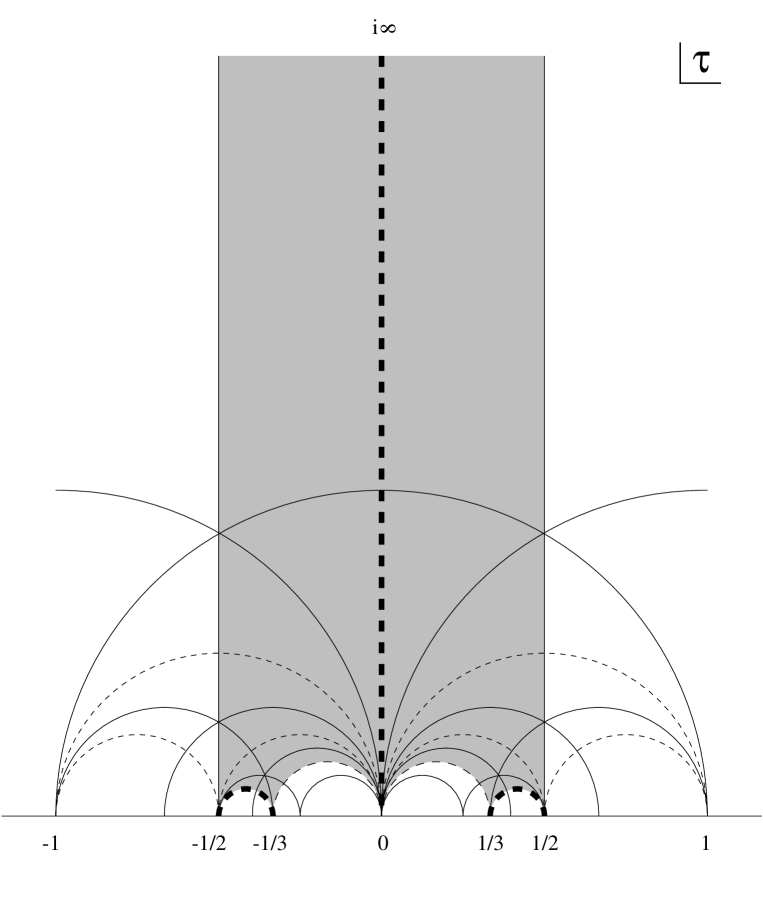
Figure 1: Fundamental domain in $\tau=\chi+i/g_{s}$ of the D1-D5 CFT for $N=6$. Corresponding boundary segments are identified under elements of $\Gamma_{0}(6)$ (in this example, the identified segments are symmetric about the imaginary axis). Heavy dashed lines denote the subspaces where the spacetime CFT becomes singular.The line from $\tau=0$ to $i\infty$ is the singular locus for $(d_{1},d_{5})=(1,6)$ or $(6,1)$, with the lower end corresponding to the former charge assignment and the upper end corresponding to the latter. Similarly, the circular arc from $\tau=1/3$ to $1/2$ is the singular locus for charges $(3,2)$ and $(2,3)$, respectively. Each rational cusp corresponds to a different weak-coupling limit of the spacetime CFT.

Thus, the residual transformations preserving the D1-D5 charge vector $(N,1)$ and lying in the particular $SO(2,2;{\bf Z})$ subgroup of U-duality is a certain ‘diagonal’ $\Gamma_{0}(N)$. The index of $\Gamma_{0}(N)$ in $\Gamma=SL(2,{\bf Z})$ (the number of copies of the $SL(2,{\bf Z})$ fundamental domain in a fundamental domain of $\Gamma_{0}(N)$) is [26]

$$(\Gamma:\Gamma_{0}(N))=N\prod_{p|N\atop p~{}{\rm prime}}(1+p^{-1})~{}.$$ (46)

The number of inequivalent rational cusps in the fundamental domain (i.e. $SL(2,{\bf Z})$ images of $\tau=i\infty$ that are not equivalent under $\Gamma_{0}(N)$) is [26]

$$\sigma_{\infty}(N)=\sum_{q|N}\varphi({\rm gcd}(q,N/q))\ ,$$ (47)

where $\varphi(n)$ is the Euler function

$$\varphi(n)=n\prod_{p|n\atop p~{}{\rm prime}}(1-p^{-1})\ .$$ (48)

We specialize to the case where the prime decomposition of $N$ contains no prime factor with multiplicity more than one; this guarantees that any partition of $N=d_{1}d_{5}$ into $(d_{1}=q,d_{5}=N/q)$ is such that $d_{1}$ and $d_{5}$ are relatively prime, so that the brane system is confined to the Higgs branch for generic moduli (the extension to general $N$ is certainly of interest but lies outside the scope of the present work). In this case $\sigma_{\infty}(N)$ is simply the number of divisors of $N$, i.e. precisely the number of ways of partitioning $N$ into two factors $(d_{1},d_{5})$. The cusps of the fundamental domain are simply those that contain the two ends of the arcs (45) for the various partitions $(d_{1},d_{5})$. The charges $(d_{1},d_{5})$ and $(d_{5},d_{1})$ are interchanged by the transformation $\tau\rightarrow-1/\tau$ and ${\tilde{\tau}}\rightarrow-1/{\tilde{\tau}}$. Hence the segment $1<t<\infty$ of the arc (45) can be assigned to the former charges, and the segment $0<t<1$ to the latter charges. Moreover, $d_{5}$ copies of the $SL(2,{\bf Z})$ fundamental domain meet at the cusp at $t=\infty$ along this arc, and $d_{1}$ copies meet at the $t=0$ cusp at the other end of the arc (see Figure 1); this reflects the periodicity of $\chi$ in the respective original U-duality frames, before the map to canonical charges $(N,1)$. The cusps are the ‘large volume limits’ of the torus $v_{4}/g_{s}\rightarrow\infty$, before the transformation (43) to the canonical frame, for different pairs of charges $(d_{1}=q,d_{5}=N/q)$; we see there is precisely one for each charge assignment. Each large volume limit is a different weak coupling limit for the dual CFT. The different limits are connected through regions of strong coupling. The fundamental domain of $\Gamma_{0}(N)$ contains all of the structure needed to describe the different D1-D5 bound states in the context of a single connected moduli space.

To summarize, we have completely and explicitly characterized the moduli space and its singular locus. With only the moduli $g_{s}$, $v_{4}/g_{s}$, $\chi$, and $A_{4}$ activated, the singular locus is given by the arcs (45); we can then switch on all the other moduli while preserving the fixed scalar conditions (10-12). Each arc in the $\tau$-plane fundamental domain of $\Gamma_{0}(N)$ gives a single connected component of the singular locus, of codimension four in the full moduli space. In particular, there are only as many disconnected components of the singular locus as there are partitions of $N$ into unordered pairs $(d_{1},d_{5})$ (for the class of examples considered here). All weak-coupling regions of the CFT other than that for $d_{1}=N$ occur along the real axis of $\tau$; these will be small-volume limits in the target space of the symmetric product (see section 6).

Up to this point we have focussed on the moduli $\tau=\chi+i/g_{s}$ and ${\tilde{\tau}}=A_{4}+iv_{4}/g_{s}$ in the map to the canonical background, by taking $B^{+}=0$. However, the disjoint (disconnected) nature of the singular loci for different $(d_{1},d_{5})$ is a property of generic moduli. The simplest argument leading to this conclusion proceeds in the F1/NS5 duality frame. We consider a singular locus which is a transformation to the canonical frame of the point $\chi=C^{+}=0$ in the background $(f_{1},n_{5})$; and another singular locus which is the analogous transformation to the canonical frame from the background $(f_{1}^{\prime},n_{5}^{\prime})$ (with $f_{1}n_{5}=f_{1}^{\prime}n_{5}^{\prime}$ and $f_{1}^{\prime}\neq n_{5}$). We want to determine whether these two co-dimension four surfaces intersect. Assume that they do, and pull some point on the intersection back to the original frame using the maps corresponding to the two inequivalent interpretations; this gives two points on the original singular surface corresponding to the charges $(f_{1},n_{5})$ and $(f_{1}^{\prime},n_{5}^{\prime})$. This surface has $\chi=C^{+}=0$ so, after taking the fixed scalar conditions in to account, it is parametrized by the standard moduli $G_{ij}+B_{ij}$ (and $g_{6}$); it is left invariant only by standard T-duality transformations. However, this is a contradiction: $(f_{1},n_{5})$ and $(f_{1}^{\prime},n_{5}^{\prime})$ are not equivalent under T-duality. We conclude that the singular surfaces do not intersect.

The case of general moduli can also be analyzed from a different point of view. After the map to the canonical frame with charges $(d_{1}d_{5},1)$, the group ${{\cal H}_{\vec{q}}}$ preserving the background tensor charge vector $\vec{q}$ is generated by two canonical subgroups: (i) the further $\Gamma_{0}(N)$ transformations (44); and (ii) transformations $ST_{\alpha}S$, where $S$ is type IIB S-duality, and $T_{\alpha}$ is an element of the $SO(4,4;{\bf Z})$ T-duality group. In other words, any element can be described via its action on the vectors of the charge lattice, and we can use T-duality to rotate a given vector into some sublattice acted on by an $SO(2,2;{\bf Z})$ subgroup that mixes it with $(d_{1},d_{5})$. The allowed transformations in this $SO(2,2;{\bf Z})$ subgroup are the image of $\Gamma_{0}(N)$ under the T-duality map.

The puzzles concerning the “level” of the current algebras, discussed heuristically in section 2, can be explained in detail using the picture developed in this section. The point is that the concept of level is meaningful only on the singular loci, where the simple formula (5) for the energy of vector excitations applies. Even with this restriction, the values of the levels are ambiguous: they are covariant under $SO(5,4;{\bf Z})$ transformations so their values ($q_{1}$ and $q_{5}$) are those of the specific singular locus. More importantly, since the different singular loci are continuously related through the bulk of moduli space the levels are indeterminate at generic points in moduli space.

The above analysis of the global structure of the D1-D5 moduli space carries over without significant modification to the case of compactification on K3; in the generators of ${{\cal H}_{\vec{q}}}$ discussed above, one simply replaces the $SO(4,4;{\bf Z})$ T-duality group in transformations of type (ii) by the $SO(4,20;{\bf Z})$ T-duality group of K3.

6 Comparison with the symmetric orbifold CFT

The analysis of the U(1) mass formula gives a great deal of robust, nontopological data about the spacetime CFT. This data can be used to pin down the relation between the symmetric orbifold CFT ${\sl Sym}^{N}(X^{4})$ and the spacetime CFT dual to $AdS_{3}\times S^{3}\times X^{4}$. The points of comparison of this CFT with the data of the spacetime CFT of the D1-D5 system consist of

• The spectrum of BPS states;

• The qualitative density of states in the vicinity of the orbifold locus;

• The moduli-dependent $U(1)^{16}$ mass formula.

In this section, we analyze these data in turn.

First, we review the spectrum of half-BPS states of the symmetric orbifold conformal field theory; it matches several previous investigations of this spectrum [13, 14, 27, 28]. As argued by Vafa [13] the half-BPS spectrum of the D1-D5 system is expected to match that of a fundamental string with winding and momentum charges (the so-called Dabholkar-Harvey spectrum). This relation is most easily seen [15] via the chain of dualities involved in maintaining a proper low-energy description of the near-horizon region as one passes to the core of the geometry; these dualities map D1/D5 charge to momentum/fundamental string winding charge. In addition, we will find a direct map between the BPS chiral vertex operators of the symmetric orbifold, and those constructed in a perturbative string approach [30, 18]; the latter, however, do not cover the full BPS spectrum, as explained in [12]. The precise match of the symmetric orbifold BPS spectrum (including the cutoff in R-charge at $j=d_{1}d_{5}/2$) limits one’s ability to tinker with this CFT and still match the structure of the unadulterated D1-D5 system.

The BPS spectrum is topological data, and as such does not help us discover where the symmetric orbifold lies in the moduli space analyzed in previous sections. The fact that it contains a $U(1)^{4}_{L}\times U(1)^{4}_{R}$ current algebra of level $N=d_{1}d_{5}$ suggests it is somewhere in the $\tau=i\infty$ cusp of the fundamental domain (c.f. Figure 1), according to the discussion of section 5. Further support for this idea comes from consideration of the non-BPS spectrum. An estimate [16] of this spectrum yields Hagedorn growth $S\propto E$ in the neighborhood of the orbifold locus. This estimate is also consistent with $q_{5}=1$.

Finally, we come to the spectrum of $U(1)^{16}$ charged states. We find a slight modification of the symmetric orbifold which precisely agrees with the formula for vector masses at $\chi={1\over 2}$ and $B=0$, and identify the perturbations away from the orbifold point in the moduli space.

6.1 The spectrum, BPS and otherwise

The symmetric orbifold whose target space is ${\sl Sym}^{N}(X^{4})$, where $X^{4}$ is K3 or $T^{4}$, is an ${\cal N}=(4,4)$ conformal field theory. In this CFT, there is a huge list of BPS states; the ground state in each twisted sector will be in a short multiplet. There is an independent twisted sector for each conjugacy class in the orbifold group, i.e. in the present case for each type of word in the symmetric group. Words are composed of cycles, each of which is a cyclic permutation of copies of $X^{4}$. The twist operator for a single cycle is the analogue of a single-trace operator in the 3+1d superYang-Mills/$AdS_{5}\times S^{5}$ duality – in other words, it is the representation of a single-particle operator. Twist operators for words that are products of cycles are multiparticle operators; their structure is determined combinatorically, and obeys the upper cutoff $j\leq N/2$ of the allowed R-charges (since a word in $S_{N}$ always has length less than or equal to $N$). Thus we need only consider the twist operators for cycles, namely the twists corresponding to

$$(X^{4})^{k}/{\bf Z}_{k}\ .$$ (49)

The twist acts by cyclic permutation of the coordinates $Y_{a\dot{a}}^{\scriptscriptstyle(\ell)}$, $\lambda_{a\alpha}^{\scriptscriptstyle(\ell)}$, $\bar{\lambda}_{a\dot{\alpha}}^{\scriptscriptstyle(\ell)}$ ($\ell=0,\dots,k-1$) of the component CFT’s; the coordinates

$${X}^{\scriptscriptstyle({\tilde{\ell}})}=\sum_{\ell=0}^{k-1}{\rm exp}\Bigl{[}2\pi i{{\tilde{\ell}}\ell\over k}\Bigr{]}Y^{\scriptscriptstyle(\ell)}\quad,\qquad{\tilde{\ell}}=0,\dots,k-1$$ (50)

diagonalize the action of the twist (similarly ${\psi}$, $\bar{\psi}$ diagonalize twists for $\lambda$, $\bar{\lambda}$). The operator which creates the twist ground state from the SL(2)-invariant CFT vacuum is the product of the $({\tilde{\ell}}/k)$ twist operators for each ${X}^{\scriptscriptstyle({\tilde{\ell}})}$, ${\tilde{\ell}}=1,...,k-1$ (and their fermionic partners). These component twist operators have conformal dimension $\Delta={\tilde{\ell}}(k-{\tilde{\ell}})/k^{2}$ from the operator that twists the bosons, and $\Delta=({\tilde{\ell}}/k)^{2}$ from the fermions; combining all the twists, the total dimension is

$$\Delta_{{\bf Z}_{k}~{}\rm twist}={\textstyle{1\over 2}}(k-1)~{}.$$ (51)

Since the dimension equals the R-charge, the operator is BPS. We will denote the chiral part of the resulting operator $\Sigma^{\alpha_{1}\cdots\alpha_{k-1}}$, exhibiting its left-handed SU(2) R-symmetry transformation as a spin ${\textstyle{1\over 2}}(k-1)$ representation. The right-handed chiral vertex operator is similarly $\bar{\Sigma}_{\dot{\alpha}_{1}\cdots\dot{\alpha}_{k-1}}$.

Details for $X^{4}=T^{4}$:

The highest weight ${\cal N}=(4,4)$ vertex operators that create single-particle BPS states are then built out of the twist operator $\Sigma\bar{\Sigma}$, together with the diagonal fermions ${\psi}^{\scriptscriptstyle(0)}$, $\bar{\psi}^{\scriptscriptstyle(0)}$ which are invariant under the twist; one simply uses these ingredients to build operators whose dimension is equal to their SU(2) spin. Bosonic operators are

$$\Phi_{0,0} = \Sigma^{\alpha_{1}\cdots\alpha_{n}}\cdot\bar{\Sigma}_{\dot{\alpha}_{1}\cdots\dot{\alpha}_{n}}$$

$$\Phi_{1,1}^{ab} = {\psi}_{\scriptscriptstyle(0)}^{a(\alpha_{1}}\Sigma^{\alpha_{2}\cdots\alpha_{n})}\cdot\bar{\psi}^{\scriptscriptstyle(0)\,b}_{(\dot{\alpha}_{1}}\bar{\Sigma}_{\dot{\alpha}_{2}\cdots\dot{\alpha}_{n})}$$

$$\Phi_{2,0} = J_{\scriptscriptstyle(0)}^{(\alpha_{1}\alpha_{2}}\Sigma^{\alpha_{3}\cdots\alpha_{n+2})}\cdot\bar{\Sigma}_{\dot{\alpha}_{1}\cdots\dot{\alpha}_{n}}$$ (52)

$$\Phi_{0,2} = \Sigma^{\alpha_{1}\cdots\alpha_{n}}\cdot{\bar{J}}^{\scriptscriptstyle(0)}_{(\dot{\alpha}_{1}\dot{\alpha}_{2}}\bar{\Sigma}_{\dot{\alpha}_{3}\cdots\dot{\alpha}_{n+2})}$$

$$\Phi_{2,2} = J_{\scriptscriptstyle(0)}^{(\alpha_{1}\alpha_{2}}\Sigma^{\alpha_{3}\cdots\alpha_{n+2})}\cdot{\bar{J}}^{\scriptscriptstyle(0)}_{(\dot{\alpha}_{1}\dot{\alpha}_{2}}\bar{\Sigma}_{\dot{\alpha}_{3}\cdots\dot{\alpha}_{n+2})}~{},$$

where $J_{\scriptscriptstyle(0)}^{\alpha\beta}={\psi}_{\scriptscriptstyle(0)}^{a\alpha}{\psi}_{\scriptscriptstyle(0)}^{b\beta}\epsilon_{ab}$ is a current built out of the diagonal fermions and ${\bar{J}}^{\scriptscriptstyle(0)}_{\dot{\alpha}_{1}\dot{\alpha}_{2}}$ is the corresponding antiholomorphic current. An analogous set of chiral building blocks for boundary operators appears in the work of [30, 18], which describes perturbative strings near the boundary of $AdS_{3}$; the transcription of the chiral vertex operators above to their counterparts in the notation of [18] is $\Sigma\leftrightarrow{\cal W}^{-}$, ${\psi}\Sigma\leftrightarrow{\cal Y}^{\pm}$, and $J\Sigma\leftrightarrow{\cal X}^{+}$. Since the formalism of [30] describes a particular regime of the spacetime CFT [12], the set of chiral operators realized there is smaller than that of the symmetric orbifold.

Similarly, the fermionic BPS operators of the $T^{4}$ symmetric orbifold are

$$\Psi_{1,0}^{a} = {\psi}_{\scriptscriptstyle(0)}^{a(\alpha_{1}}\Sigma^{\alpha_{2}\cdots\alpha_{n+1})}\cdot\bar{\Sigma}_{\dot{\alpha}_{1}\cdots\dot{\alpha}_{n}}$$

$$\Psi_{0,1}^{a} = \Sigma^{\alpha_{1}\cdots\alpha_{n}}\cdot\bar{\psi}^{\scriptscriptstyle(0)a}_{(\dot{\alpha}_{1}}\bar{\Sigma}_{\dot{\alpha}_{2}\cdots\dot{\alpha}_{n+1})}$$

$$\Psi_{1,2}^{a} = {\psi}_{\scriptscriptstyle(0)}^{a(\alpha_{1}}\Sigma^{\alpha_{2}\cdots\alpha_{n+1})}\cdot{\bar{J}}^{\scriptscriptstyle(0)}_{(\dot{\alpha}_{1}\dot{\alpha}_{2}}\bar{\Sigma}_{\dot{\alpha}_{3}\cdots\dot{\alpha}_{n+2})}$$ (53)

$$\Psi_{2,1}^{a} = J_{\scriptscriptstyle(0)}^{(\alpha_{1}\alpha_{2}}\Sigma^{\alpha_{3}\cdots\alpha_{n+2})}\cdot\bar{\psi}^{\scriptscriptstyle(0)a}_{(\dot{\alpha}_{1}}\bar{\Sigma}_{\dot{\alpha}_{2}\cdots\dot{\alpha}_{n+1})}~{}.$$

The sixteen operators $\Phi_{p,q}$, $\Psi_{p,q}$ fill out the Hodge diamond $H^{p,q}$ of $T^{4}$ [14, 27, 28], with eight odd elements corresponding to fermions and eight even elements corresponding to bosons.

Finally, the proper description of the CFT for $X^{4}=T^{4}$ includes an additional four-torus ${\tilde{T}}^{4}$ current algebra. The BPS spectrum of this extra ${\tilde{T}}^{4}$ consists of $1$, ${\tilde{\lambda}}$, $\bar{\tilde{\lambda}}$, ${\tilde{\lambda}}\bar{\tilde{\lambda}}$; the counting of these latter states is again that of the four-torus cohomology, and is isomorphic to the set of chiral ground states of the superstring. Without this extra contribution, one would not reproduce the correct degeneracy of BPS states. The counting of multiparticle BPS states matches that of the chiral spectrum of the superstring, since the basic operators (52),(53) are isomorphic to the chiral oscillator spectrum of the superstring, and the multiparticle states are the Fock space of the single-particle spectrum. All told, the BPS spectrum is that of the (Dabholkar-Harvey) BPS states of a single superstring – the 16 BPS states from the extra $T^{4}$ supplies the degeneracy of the left-moving ground states, and the symmetric product gives the same counting as the left-moving oscillator states at level $N=d_{1}d_{5}$; the global ${\cal N}=(4,4)$ descendants supply an extra factor of 16, representing the right-moving ground state degeneracy.

Details for $X^{4}=K3$:

The situation for $X^{4}=K3$ is similar. One has exactly the same twist operators $\Sigma\cdot\bar{\Sigma}$ for $k$-cycles, which can be tensored with any of the 24 chiral primaries from the diagonal copy of K3 in $K3^{k}/{\bf Z}_{k}$; thus the structure is that of the chiral oscillators of the bosonic string. In this case all $d_{1}d_{5}+1$ copies of K3 are involved in the symmetric orbifold. There is no extra degeneracy of BPS states from some other component of the CFT, analogous to the extra $T^{4}$ in the previous example; this matches onto the uniqueness of the ground state of the bosonic string. Also, the additional copy of K3 in the symmetric product means that the degeneracy of BPS states will be that of the bosonic string at level $N=d_{1}d_{5}+1$, matching the shift by one in ground state energy. Finally, taking into account the 16-fold degeneracy of the ${\cal N}=(4,4)$ short multiplet gives the Dabholkar-Harvey spectrum of the heterotic string, as expected [13, 15]. The moduli involve the usual 20 hypermultiplets of the base K3, together with the further blowup hypermultiplet (described below for the torus case); together they parametrize the $SO(4,21)/SO(4)\times SO(21)$ Teichmuller moduli space.

Non BPS states:

A simple argument [16] shows that the full density of (generically non-BPS) NS-sector states of the symmetric orbifold is of a stringy nature, not characteristic of low-energy supergravity on $AdS_{3}\times S^{3}\times X^{4}$. The $k^{\rm th}$ twisted sector has oscillators with moding $1/k$; the energy cost to reach this sector is $R_{5}E\sim O(k)$ (see (51)). Thus the total density of states is approximately

$$\rho(E)\sim\sum_{k=1}^{\min{(d_{1}d_{5},R_{5}E)}}\rho_{k}\,{\rm exp}\Bigl{[}\beta_{0}\sqrt{k(R_{5}E-k)}\Bigr{]}~{},$$ (54)

for some constants $\beta_{0}$, $\rho_{k}$. For a given $R_{5}E<d_{1}d_{5}$, the value of $k$ that dominates the density of states is $O(R_{5}E/2)$, thus $\rho(E)\sim{\rm exp}[\beta_{0}R_{5}E/2]$ is a Hagedorn spectrum. This spectrum turns over to the ${\rm exp}[2\pi\sqrt{d_{1}d_{5}E}]$ growth required of a CFT with central charge $c=6d_{1}d_{5}$ above the characteristic energy scale $R_{5}E\sim d_{1}d_{5}$. Because the low-energy spectrum has string-theoretic rather than field-theoretic growth, the symmetric orbifold must describe a regime where there is a string in the theory whose tension is of order the AdS radius of curvature, so that the spacetime does not have a supergravity interpretation. It is not difficult to identify the culprit: In the D1-D5 background, the AdS radius in units of the D-string tension is $\sqrt{d_{5}}$, so that when $d_{5}=1$ the spacetime seen by this object has stringy curvature. One has to make sure that the spacetime is of low curvature with respect to all strings present in the spectrum in order to have a valid low-energy supergravity description. As is standard in decoupling limits, the region of the moduli space corresponding to spacetimes with a valid low-energy supergravity description is a strongly-coupled region of the dual quantum field theory. We take the qualitative agreement of the full spectrum of the symmetric orbifold with that expected for $d_{5}=1$ as further evidence for the identification of the orbifold locus with a part of the $d_{5}=1$ region of the moduli space of the spacetime CFT.

6.2 Dependence on moduli

The $U(1)^{4}_{L}\times U(1)^{4}_{R}$ of the symmetric orbifold ${\sl Sym}^{N}(T^{4})$ is at level $N=d_{1}d_{5}$, while that of ${\tilde{T}}^{4}$ is at level one. This suggests that this CFT describes some part of the corresponding region of the spacetime CFT, where the U(1) spectrum separates into two pieces with corresponding levels — in other words, the $\tau\rightarrow i\infty$ cusp of the fundamental domain in the canonical presentation of section 5. We now provide further evidence in support of this proposal, by checking that the dependence on all the moduli is consistent with this identification.

The moduli space of the ${\sl Sym}^{N}(T^{4})$ theory includes the 16 Narain moduli

$${\cal M}^{ij}=\gamma^{i}_{a\dot{a}}\gamma^{j}_{b\dot{b}}\partial Y^{a\dot{a}}\bar{\partial}Y^{b\dot{b}}~{},$$ (55)

of the $d_{1}d_{5}$ copies of $T^{4}$ in the symmetric product, as well as the four blowup modes of the ${\bf Z}_{2}$ twist in $S_{d_{1}d_{5}}$; near the orbifold point, the corresponding operators are the descendants

$${\cal M}^{ab}=G_{-1/2}^{a\alpha}\bar{G}_{-1/2}^{b\dot{\beta}}\Sigma_{\alpha}\cdot\bar{\Sigma}_{\dot{\beta}}~{},$$ (56)

of the ${\bf Z}_{2}$ twist highest weight. In addition to these 20 moduli parametrizing ${\cal K}=SO(5,4)/SO(5)\times SO(4)$, there are the U(1) current perturbations ${\cal J}_{i}\overline{\cal J}_{j}$, ${\widetilde{\cal J}}_{i}\overline{\cal J}_{j}$, ${\cal J}_{i}{\overline{\widetilde{\cal J}}}_{j}$, and ${\widetilde{\cal J}}_{i}{\overline{\widetilde{\cal J}}}_{j}$, where ${\cal J}_{i}$, $\overline{\cal J}_{i}$ are the eight diagonal U(1) currents of $(T^{4})^{N}$; and ${\widetilde{\cal J}}_{i}$, ${\overline{\widetilde{\cal J}}}_{i}$ are the U(1) currents of the ${\tilde{T}}^{4}$. One issue we will have to address is precisely how the moduli space of the spacetime theory sits inside this 84-dimensional moduli space.

To begin, let us turn off the self-dual NS B-field moduli in the U(1) spectrum formula (21) (with the shifts (22) implied). Let $d_{1}=N$ and $d_{5}=1$, and define the unit volume metric ${\hat{G}}_{ij}=G_{ij}/\sqrt{v_{4}}$ and six-dimensional string coupling $g_{6}=g_{s}/\sqrt{v_{4}}$. The U(1) mass formula reduces to

$$R_{5}M = {1\over 2N}\Bigl{[}(p_{i}-C_{ik}w^{k}_{D1}+N\chi w^{D3}_{i})\cdot g_{6}{\hat{G}}^{ij}\cdot(p_{j}-C_{jm}w^{m}_{D1}+N\chi w^{D3}_{j})$$ (57)

$$\qquad\qquad+w_{D1}^{i}\cdot g_{6}^{-1}{\hat{G}}_{ij}\cdot w_{D1}^{j}+2p_{i}w^{i}_{D1}\Bigr{]}$$

$$+{1\over 2}\Bigl{[}(w_{F1}^{i}-{{}^{*}C}^{ik}w^{D3}_{k}-\chi w_{D1}^{i})\cdot g_{6}{\hat{G}}_{ij}\cdot(w_{F1}^{j}-{{}^{*}C}^{jm}w^{D3}_{m}-\chi w_{D1}^{j})$$

$$\qquad\qquad+w^{D3}_{i}\cdot g_{6}^{-1}{\hat{G}}^{ij}\cdot w^{D3}_{j}-2w^{i}_{F1}w_{i}^{D3}\Bigr{]}~{}.$$

The $SO(4,4)/SO(4)\times SO(4)$ moduli parametrized by $g_{6}$, ${\hat{G}}$, and $C_{ij}$ appear differently in the two square brackets. This is because the eight U(1) charges $(p_{i},w_{D1}^{i})$ transform in the vector of the associated $SO(4,4;{\bf Z})$ T-duality group, while the eight charges $(w^{i}_{F1},w^{D3}_{i})$ transform in a spinor representation (the two are related by triality in SO(4,4)). In terms of this data, we identify the moduli of the tori in the symmetric orbifold as a metric $g_{6}^{-1}{\hat{G}}_{ij}$ and an antisymmetric tensor $C_{ij}$, whereas the moduli of the extra ${\tilde{T}}^{4}$ are a metric $g_{6}^{-1}{\hat{G}}^{ij}$ and an antisymmetric tensor ${{}^{*}C}^{ij}=\epsilon^{ijkl}C_{kj}$. Note also that, even though $w_{F1}^{i}$ has a contravariant index, it should be thought of as a ‘momentum’ charge on ${\tilde{T}}^{4}$ for the present purpose, since it is this quantity that is shifted by the ${\tilde{T}}^{4}$ ‘winding’ $w^{D3}_{i}$ in the presence of a nontrivial antisymmetric tensor background.

Having found the embedding of the $SO(4,4)/SO(4)\times SO(4)$ moduli of the spacetime CFT in that of the $(SO(4,4)/SO(4)\times SO(4))^{2}$ moduli space of tori of the ${\sl Sym}^{N}(T^{4})\times{\tilde{T}}^{4}$ CFT, we can account for the $\chi$ dependence as follows. From the way it appears in (57), part of the perturbation corresponding to $\chi$ should be another antisymmetric tensor modulus of ${\sl Sym}^{N}(T^{4})\times{\tilde{T}}^{4}$ since it couples in the same way; however, since it couples the momentum of ${\sl Sym}^{N}(T^{4})$ to the winding on ${\tilde{T}}^{4}$ and vice-versa, it must involve an antisymmetric perturbation that mixes the two factors. The fact that the orbifold is parity symmetric means that it can only describe $\chi=0$ or $\chi={1\over 2}$ in the moduli space [22]. However, $\chi=0$ is a singular CFT, leaving $\chi={1\over 2}$ as the only candidate. Thus we should modify the orbifold to include an asymmetric shift by half a lattice vector coupling ${\cal J}_{i}$ and ${\widetilde{\cal J}}_{i}$. Note that this asymmetric shift will copy the winding $w^{D3}_{i}$ on the ${\tilde{T}}^{4}$ onto each copy of $T^{4}$ in the symmetric product, accounting for the relative factor of $N$ in shift of the momenta in the first term of (57). The asymmetric shift amounts to turning on a term

$$\widehat{\cal M}=\Bigl{(}{\cal J}^{a\dot{a}}{\overline{\widetilde{\cal J}}}^{b\dot{b}}-{\widetilde{\cal J}}^{a\dot{a}}\overline{\cal J}^{b\dot{b}}\Bigr{)}\epsilon_{ab}\epsilon_{\dot{a}\dot{b}}~{},$$ (58)

in the action of the sigma model on ${\sl Sym}^{N}(T^{4})\times{\tilde{T}}^{4}$. However, the vertex operator corresponding to the modulus $\chi$ cannot consist solely of $\widehat{\cal M}$, since deforming the orbifold to $\chi=0$ would not result in a singular CFT. This job is accomplished by the scalar ${\bf Z}_{2}$ blowup mode $\epsilon_{ab}{\cal M}^{ab}$ (56), which also has the right quantum numbers to be part of the modulus $\chi$. Moreover, it is the operator that shifts the theta angle in the symmetric orbifold sigma model; turning it on by half a unit tunes the theta angle to zero, resulting in the singular CFT expected at $\chi=0$. Thus the dependence of the spacetime CFT on the modulus $\chi$ is carried by several different parts of the symmetric orbifold – the blowup modulus accounts for the singularity encountered at $\chi=0$, while the current-current perturbation $\widehat{\cal M}$ takes care of the mixing of U(1) charges as a function of $\chi$. The correct perturbation away from the orbifold point is $\delta\chi\cdot(\widehat{\cal M}+\epsilon_{ab}{\cal M}^{ab})$.

The analysis for the other three blowup moduli (self-dual NS two-forms in the present duality frame) is similar, but complicated by the fact that these perturbations enter as metric deformations in the U(1) mass formula. Indeed, they couple the ‘momenta’ $p_{i}$ and $w_{F1}^{i}$ to one another, as well as the ‘winding’ quantum numbers $w_{D1}^{i}$ and $w^{D3}_{i}$. It is natural to identify the perturbations away from the orbifold point with the symmetric combinations

$$\vec{\cal M}=\Bigl{(}{\cal J}^{a\dot{a}}{\overline{\widetilde{\cal J}}}^{b\dot{b}}+{\widetilde{\cal J}}^{a\dot{a}}\overline{\cal J}^{b\dot{b}}\Bigr{)}\vec{\tau}_{ab}\epsilon_{\dot{a}\dot{b}}~{}.$$ (59)

It is not too hard to check that, to lowest order, the effect on the symmetric product is $N$ times that on the extra ${\tilde{T}}^{4}$, just as for the $\chi$ perturbation. In any case, these moduli are turned off at the orbifold locus (otherwise, they would break various discrete symmetries). The perturbation away from the orbifold locus is $\delta{\vec{B}^{+}}\cdot(\vec{\cal M}+{\vec{\tau}}_{ab}{\cal M}^{ab})$.

To summarize, we propose that the orbifold ${\sl Sym}^{N}(T^{4})\mathbin{\hbox{\hskip 2.0pt\vrule height=5.5pt,depth=-0.3pt,width=0.4pt\hskip-2.0pt$\times$}}{\tilde{T}}^{4}$, where the semi-direct product is meant to indicate the additional asymmetric shift coupling the two factors, describes the line $\chi={1\over 2}$ in the D1-D5 moduli space in the canonical duality frame of section 5. Moving in the moduli subspace parametrized by $\chi$ and $g_{6}=g_{s}/\sqrt{N}$, we should encounter the singularities corresponding to all other partitions of $N$. These loci depend separately on $d_{1}$ and $d_{5}$, and we get a different singular locus in the moduli space of the symmetric product, for each possible partition of the product $N=d_{1}d_{5}$ into two factors. All the other singularities are at small volume of the $T^{4}$, with order one amount of the blowup modulus turned on; thus the sigma model is strongly coupled.

It would be interesting to understand what phenomenon in the CFT distinguishes the singular domains; it is natural to speculate that there is a singularity in the sigma model target space in which $d_{5}$ ‘fractional instantons’ come together to make a D1-brane or D5-brane that leaves the system, and that this phenomenon is related to the denominators of the rational cusps of the fundamental domain – i.e. that $\chi\sim a/d_{1}$ or $\chi\sim b/d_{5}$ (in the notation of section (5)). Perhaps these are relics of the $d_{1}$- or $d_{5}$-twisted sectors of the orbifold, since the ‘fractional instantons’ at the orbifold point are the fields parametrizing the component copies of $T^{4}$; and it is these twist operators that sew together the proper number of ‘fractional instantons’ of the orbifold theory to reconstitute a string that can leave the system. It is hard to be precise, however, since the orbifold point is far in the moduli space from the singular loci.

6.3 Other orbifolds

Adding KK monopoles: In [18], the GKS formalism was extended to the ${\cal N}=(4,0)$ SCFT obtained when one introduces Kaluza-Klein monopoles into the brane background, after compactification on an additional circle. The moduli space of the IIB theory on $T^{5}$ is $E_{6(6)}/USp(8)$, which is restricted to $F_{4(4)}/SU(2)\times USp(6)$ by the fixed scalar mechanism. Analogous to the D1-D5 system without the KK monopole, the group of discrete identifications of the moduli space is the subgroup of $E_{6(6)}({\bf Z})$ that fixes the background charges. It would be interesting to give a more explicit characterization of it, along the lines of the present discussion for the D1-D5 background. In the symmetric orbifold CFT, the addition of $p$ KK monopoles to the background involves an asymmetric orbifold that acts as a ${\bf Z}_{p}$ twist of the right-moving SU(2) R-symmetry [18, 33]. This twist breaks the right-moving supersymmetry completely, consequently there will be additional moduli which involve lowest components of superfields from the untwisted sector (one can check that no new moduli arise from twisted sectors of the ${\bf Z}_{p}$ orbifold). Near the orbifold point, the additional moduli are generated by the vertex operators

$${\cal M}_{a\dot{a}\,5}=\partial Y_{a\dot{a}}\bar{J}_{3}~{},$$ (60)

(here $J_{3}$ is the R-current left unbroken by the ${\bf Z}_{p}$ action), and by

$$\widetilde{\cal M}^{ab}=G_{-1/2}^{a\alpha}\Sigma_{\alpha}\cdot\bar{\psi}_{\scriptscriptstyle(0)}^{b\dot{\beta}}\bar{\Sigma}^{\dot{\alpha}}\tau^{3}_{\dot{\alpha}\dot{\beta}}~{}.$$ (61)

It is not difficult to check that these operators have no three-point function with themselves, the $T^{4}$ moduli, or the blowup modes (56), and are thus moduli (this should be a sufficient condition given $(4,0)$ supersymmetry). They also have the right spacetime quantum numbers under both Lorentz and $SU(2)\times USp(6)$ transformations. Specifically, the moduli transform as the $(2,14)$ under this group, which decomposes as a $(2,1,4)\oplus(2,2,5)$ under the manifest $SU(2)\times SU(2)\times SO(5)$ of the orbifold CFT (the $SU(2)\times SU(2)$ transforms the left-movers of the CFT, the SO(5) the right-movers); the (2,2,5) consist of the moduli from the untwisted sector, and the (2,1,4) are the eight moduli (56),(61) coming from the ${\bf Z}_{2}$ twisted sector of the symmetric orbifold.

One can again carry out the scaling analysis of section 2. The type IIB theory is now compactified on $T^{6}$, with one circle kept large and the rest having sizes of order the string scale. There is a background of three of the 27 available tensor charges turned on, which we have taken to consist of $p$ KK monopoles, $q_{5}$ D5-branes, and $q_{1}$ D-strings. The background naturally distinguishes one of the five small circles as the nontrivial fiber of the KK monopole; the remaining four are isomorphic to the $T^{4}$ that the D1-D5 system is compactified on. The vector excitations about the background form a ${\bf 27}$ of the $E_{6(6)}$ duality group of the small $T^{5}$: ${5\choose 3}=10$ D3-branes, 5 D1-branes, 5 fundamental strings, 5 KK-momenta, one wrapped D5-brane, and one wrapped NS5-brane. These naturally decompose as $\bf 8_{v}+8_{s}+8_{c}+1+1+1$ under the $SO(4,4)$ T-duality group of the $T^{4}$. One finds a structure reminiscent of (5), with three separate $T^{4}$ current algebras of levels $q_{1}$, $q_{5}$, and $p$; and an interesting triality symmetry among the terms. We hope to give further details elsewhere.

Orientifolds: One can also consider the D1-D5 system in the presence of an orientifold plane. In this case, the orientifold projection eliminates the RR scalar and the four-form $A_{4}$, as well as the NS B-field. Therefore, the $SO(5,4)/SO(5)\times SO(4)$ near-horizon moduli space will be reduced to $SO(4,4)/SO(4)\times SO(4)$; the RR scalar will be frozen to either $\chi=0$ or $\chi={1\over 2}$ for any given values of $d_{1}$ and $d_{5}$. In particular, the moduli that enabled us to move between the various domains associated to different one-brane and five-brane charges for fixed $N=d_{1}d_{5}$ are projected out. Any orbifold conformal field theory that describes such a situation then has no analogues of the twisted sector moduli ${\cal M}^{ab}$; the orbifold moduli space will then only describe $d_{1}=1$ or $d_{5}=1$.

A general analysis of D5-branes in the presence of orientifold 5-planes was performed in [34, 35, 36]. There are two types of orientifold that fix $\chi=0$ and two that fix $\chi={1\over 2}$; only the latter are expected to lead to nonsingular dual CFT’s when D1-branes are added and the scaling limit is taken. These are

• An O5-plane of SO-type (D5-brane charge -1) with an odd number of 5-branes, yielding gauge group $SO(2k+1)$;

• An O5-plane of Sp-type (D5-brane charge +2) with an even number of D5-branes, giving $Sp(2k)$ gauge group.

One might therefore expect that there is an appropriate modification of the symmetric orbifold that generates the moduli space of a single $SO(2k+1)$ or $Sp(2k)$ instanton on $T^{4}$ or K3. The dimension of the moduli space of $n$ instantons in $SO(2k+1)$ or $Sp(2k)$ gauge theory on $T^{4}$ or K3 is $4[2k(n-k)-k]$, leading one to expect a CFT of central charge $c=6[2d_{1}d_{5}-d_{5}]$, in particular one has $c=6d_{5}$ when $d_{1}=1$. The orientifold will eliminate all half-integer spin representations of R-symmetry from the half-BPS spectrum. It is this projection that removes the twisted moduli ${\cal M}^{ab}$ (56) related to $\chi$ and $B^{+}$, pinning the orbifold at $\chi={1\over 2}$. Since the projection eliminates the gauge fields that carry fundamental string and D3-brane flux, when $X^{4}=T^{4}$, only the U(1) charges associated to momenta and wrapped D1-branes survive.

Acknowledgments: We wish to thank A. Dabholkar, R. Dijkgraaf, J. Harvey, A. Hashimoto, T. Hollowood, J. Maldacena, A. Strominger, and particularly D. Kutasov for helpful discussions; and the Harvard University theory group and the ITP, Santa Barbara for hospitality during the course of our investigations. This work was supported by DOE grant DE-FG02-90ER-40560. F.L. is supported in part by a McCormick Fellowship.

Appendix A Derivation of a BPS formula

The mass formulae of interest are BPS formulae, and hence direct consequences of supersymmetry. BPS masses are derived by solving appropriate eigenvalue problems. The details of this strategy as well as original references can be found in the review [21].

The simplest starting point is the expression for the supersymmetry algebra in M-theory. Imposing nontrivial supersymmetry leads to an eigenvalue equation for the central charges

$$\left[{\cal C}\Gamma^{M}P_{M}+{1\over 2}{\cal C}\Gamma^{MN}Z_{MN}+{1\over 5!}{\cal C}\Gamma^{MNPQR}Z_{MNPQR}\right]\epsilon=0~{}.$$ (62)

The central charges $Z_{MN}$ and $Z_{MNPQR}$ are M2- and M5-brane charges, respectively, and the $P_{M}$ are the momenta; in particular $P_{0}$ is the mass $M$ that we want to compute. The parity-odd moduli are taken to vanish; they will be reinstated in the end. $\epsilon$ is the spinorial eigenvector of the preserved supersymmetry. The metric is mostly plus.

In this Appendix we consider a F1/NS5 background and excitations with arbitrary vector charges. Our charge assignments are type IIB but transformation to M-theory is simple; this leads to the eigenvalue equation

$$\left[\Gamma^{5}Q_{1}+\Gamma^{1234}\Gamma^{5}Q_{5}+\Gamma^{i}P_{i}+\Gamma_{i}\Gamma^{11}W^{i}_{F1}+\Gamma_{i}\Gamma^{5}W^{i}_{D1}+\Gamma^{5}\Gamma^{11}\Gamma^{1234}\Gamma^{i}W_{i}^{D3}\right]\epsilon=\Gamma^{0}M\epsilon$$ (63)

The physical charge, denoted by a capital letter, is the mass of an isolated brane with the given charge. The masses (1) therefore give the conversion factors between the physical charges used here, and the quantized charges used in the main text.

The square of the eigenvalue equation gives the expression for the mass

$$M^{2}=M^{2}_{T}+M^{2}_{V}+2M_{TV}~{},$$ (64)

where

$$M^{2}_{T}=Q^{2}_{1}+Q^{2}_{5}+2Q_{1}Q_{5}\Gamma^{1234}~{},$$ (65)

is the contribution of the background,

$$M^{2}_{V} = \vec{P}^{2}+\vec{W}^{2}_{F1}+\vec{W}^{2}_{D1}+\vec{W}^{2}_{D3}$$ (66)

$$\quad+2\Bigl{[}\Gamma^{11}\vec{P}\cdot\vec{W}_{F1}+\Gamma^{5}\vec{P}\cdot\vec{W}_{D1}$$

$$\qquad\qquad-\Gamma^{11}\Gamma^{1234}\vec{W}_{D1}\cdot\vec{W}_{D3}+\Gamma^{5}\Gamma^{1234}\vec{W}_{F1}\cdot\vec{W}_{D3}$$

$$\qquad\qquad\qquad+\Gamma^{5}\Gamma^{11}\Gamma_{ij}W^{i}_{D1}W^{j}_{F1}+\Gamma^{5}\Gamma^{11}\Gamma^{1234}\Gamma^{ij}W_{i}^{D3}P_{j}\Bigr{]}~{},$$

is the contribution of the vector excitations, and

$$M_{TV} = Q_{1}\left[-\Gamma_{i}W^{i}_{D1}+\Gamma_{11}\Gamma^{1234}\Gamma^{i}W_{i}^{D3}\right]$$ (67)

$$+ Q_{5}\left[\Gamma^{5}\Gamma^{1234}\Gamma^{i}P_{i}-\Gamma^{5}\Gamma^{11}\Gamma^{1234}\Gamma_{i}W^{i}_{F1}\right]~{},$$

is an interaction term between the background and the excitations. In these equations it is implied that all gamma-matrices act on $\epsilon$, even though this is not indicated explicitly.

At this point the manipulations simplify upon taking the scaling limit into account. $M_{T}^{2}$ is order $l_{s}^{-4}$, $M_{V}^{2}$ is order $l_{s}^{-2}$, and $M_{TV}$ is order $l_{s}^{-3}$. The square of the largest terms is

$$(Q_{1}Q_{5}\Gamma^{1234}+M_{TV})^{2} = Q_{1}^{2}Q_{5}^{2}+Q^{2}_{5}(\vec{P}^{2}+\vec{W}^{2}_{F1}+2\Gamma^{11}\vec{P}\cdot\vec{W}_{F1})$$

$$\quad+Q^{2}_{1}(\vec{W}^{2}_{D1}+\vec{W}^{2}_{D3}-2\Gamma^{11}\Gamma^{1234}\vec{W}_{D1}\cdot\vec{W}_{D3})$$

$$\quad+2Q_{1}Q_{5}\left(-\Gamma^{5}\Gamma^{1234}\vec{P}\cdot\vec{W}_{D1}-\Gamma^{5}\vec{W}_{F1}\cdot\vec{W}_{D3}\right.$$

$$\quad\qquad\left.\Gamma^{5}\Gamma^{11}\Gamma^{1234}\Gamma_{ij}W^{i}_{F1}W^{j}_{D1}+\Gamma^{5}\Gamma^{11}\Gamma^{ij}P_{i}W_{j}^{D3}\right)~{},$$

Note that $\Gamma^{1234}$ anticommutes with $M_{TV}$ so that there are no terms of order $l_{s}^{-3}$. It is this structure of the supersymmetry which is ultimately responsible for the vector charges having finite energy in the scaling limit.

Next, take the square root and expand

$$Q_{1}Q_{5}\Gamma^{1234}+M_{TV} \simeq Q_{1}Q_{5}+{Q_{1}\over 2Q_{5}}(\vec{W}^{2}_{D1}+\vec{W}^{2}_{D3}-2\Gamma^{11}\vec{W}_{D1}\cdot\vec{W}_{D3})$$

$$\quad\quad+{Q_{5}\over 2Q_{1}}(\vec{P}^{2}+\vec{W}^{2}_{F1}-2\Gamma^{11}\vec{P}\cdot\vec{W}_{F1})$$

$$\quad\quad\quad-\Gamma^{5}\vec{P}\cdot\vec{W}_{D1}-\Gamma^{5}\vec{W}_{F1}\cdot\vec{W}_{D3}$$

$$\quad\quad\quad\quad+\Gamma^{5}\Gamma^{11}\Gamma_{ij}W^{i}_{F1}W^{j}_{D1}+\Gamma^{5}\Gamma^{11}\Gamma^{ij}P_{i}W_{j}^{D3}~{}.$$

This result is valid up to terms of order $l_{s}^{2}$. We have chosen the subspace where $\Gamma^{1234}=1$, as appropriate when $Q_{1},Q_{5}>0$; this is legitimate at this point because $\Gamma^{1234}$ commutes with all other operators that remain. The terms in (64) now add to

$$M^{2} = (Q_{1}+Q_{5})^{2}+{Q_{1}+Q_{5}\over Q_{5}}(\vec{W}^{2}_{D1}+\vec{W}^{2}_{D3}-2\Gamma^{11}\vec{W}_{D1}\cdot\vec{W}_{D3})$$ (70)

$$\quad+{Q_{1}+Q_{5}\over Q_{1}}(\vec{P}^{2}+\vec{W}^{2}_{F1}+2\Gamma^{11}\vec{P}\cdot\vec{W}_{F1})~{},$$

up to order $l_{s}^{2}$. Note that this simple expression is the result of numerous cancellations between the vector terms and the tensor-vector interactions. At this point the eigenvalue equation is solved by taking $\Gamma^{11}=1$ (this is legitimate because it commutes with $\Gamma^{1234}=1$). Taking the square root again gives

$$M = Q_{1}+Q_{5}+{1\over 2Q_{5}}(\vec{W}^{2}_{D1}+\vec{W}^{2}_{D3}-2\vec{W}_{D1}\cdot\vec{W}_{D3})$$ (71)

$$\quad+{1\over 2Q_{1}}(\vec{P}^{2}+\vec{W}^{2}_{F1}-2\vec{P}\cdot\vec{W}_{F1})~{}.$$

The excitation energy can now be read off as the energy above the background mass. After conversion to the quantized charges used in the main text, the result reads

$$ER_{5}={1\over 2f_{1}}~{}(\vec{p}+\vec{w}_{F1})^{2}+{1\over 2n_{5}}~{}{1\over v_{4}}~{}(\vec{w}_{D1}-v_{4}\vec{w}_{D3})^{2}~{}.$$ (72)

Here it is understood that $G^{ij}$ (contracting $p_{i}$, $w_{i}^{D3}$) and $G_{ij}$ (contracting $w^{i}_{F1}$, $w^{i}_{D1}$) are measured in units of $l_{s}$. The final equation (72) is identical to (21), except that the sign of $\vec{w}_{D3}$ has been changed. This is purely a matter of conventions.

Two refinements of these results are needed for the entropy computation in section 4. First, it is straightforward to generalize the computation in this Appendix by including also the scalar charge $p_{5}$, i.e. the momentum along the background $F1$. The result is simply that $p_{5}$ can be added on the right-hand side of (72), without any further cross-terms. Next, the mass computed here is the largest eigenvalue of the central charge matrix. The computation also identifies the smaller eigenvalue: it is found by choosing instead $\Gamma^{11}=-1$ after (70). This results in the opposite signs within the absolute squares in (72). This justifies the smaller conformal weight ($h_{L}$) used in section 4.

References

- [1] A. Strominger and C. Vafa. Microscopic origin of the Bekenstein-Hawking entropy. Phys. Lett., B379:99–104, 1996. hep-th/9601029.
- [2] J. M. Maldacena. Black holes and D-branes. Nucl. Phys. Proc. Suppl., 61A:111, 1998. hep-th/9705078.
- [3] A. W. Peet. The Bekenstein formula and string theory (N-brane theory). Class. Quant. Grav., 15:3291, 1998. hep-th/9712253.
- [4] T. Banks, W. Fischler, S. H. Shenker, and L. Susskind. M theory as a matrix model: A conjecture. Phys. Rev., D55:5112–5128, 1997. hep-th/9610043.
- [5] J. Maldacena. The large N limit of superconformal field theories and supergravity. Adv. Theor. Math. Phys., 2:231, 1998. hep-th/9711200.
- [6] S. S. Gubser, I. R. Klebanov, and A. M. Polyakov. Gauge theory correlators from noncritical string theory. Phys. Lett., B428:105, 1998. hep-th/9802109.
- [7] E. Witten. Anti-de Sitter space and holography. Adv. Theor. Math. Phys., 2:253, 1998. hep-th/9802150.
- [8] R. Dijkgraaf. Instanton strings and HyperKahler geometry. Nucl. Phys., B543:545, 1999. hep-th/9810210.
- [9] D. Kutasov and N. Seiberg. More comments on string theory on . JHEP, 04:008, 1999. hep-th/9903219.
- [10] S. Ferrara, R. Kallosh, and A. Strominger. N=2 extremal black holes. Phys. Rev., D52:5412–5416, 1995. hep-th/9508072.
- [11] S. Ferrara and R. Kallosh. Supersymmetry and attractors. Phys. Rev., D54:1514–1524, 1996. hep-th/9602136.
- [12] N. Seiberg and E. Witten. The D1 / D5 system and singular CFT. JHEP, 04:017, 1999. hep-th/9903224.
- [13] Cumrun Vafa. Gas of D-branes and Hagedorn density of BPS states. Nucl. Phys., B463:415–419, 1996. hep-th/9511088.
- [14] J. Maldacena and A. Strominger. black holes and a stringy exclusion principle. JHEP, 12:005, 1998. hep-th/9804085.
- [15] E. Martinec and V. Sahakian. Black holes and five-brane thermodynamics. 1999. hep-th/9901135.
- [16] T. Banks, M. R. Douglas, G. T. Horowitz, and E. Martinec. AdS dynamics from conformal field theory. 1998. hep-th/9808016.
- [17] J. Maldacena, G. Moore, and A. Strominger. Counting BPS black holes in toroidal type-II string theory. 1999. hep-th/9903163.
- [18] D. Kutasov, F. Larsen, and R. G. Leigh. String theory in magnetic monopole backgrounds. 1998. hep-th/9812027.
- [19] T. Banks, N. Seiberg, and S. Shenker. Branes from matrices. Nucl. Phys., B490:91–106, 1997. hep-th/9612157.
- [20] M. R. Douglas. Branes within branes. 1995. hep-th/9512077.
- [21] N. A. Obers and B. Pioline. U duality and M theory, an algebraic approach. 1998. hep-th/9812139.
- [22] E. Witten. On the conformal field theory of the Higgs branch. JHEP, 07:003, 1997. hep-th/9707093.
- [23] J. Maldacena, J. Michelson, and A. Strominger. Anti-de Sitter fragmentation. JHEP, 02:011, 1999. hep-th/9812073.
- [24] R. Dijkgraaf, E. Verlinde, and H. Verlinde. BPS spectrum of the five-brane and black hole entropy. Nucl. Phys., B486:77–88, 1997. hep-th/9603126.
- [25] N. Dorey, T. J. Hollowood, V. V. Khoze, M. P. Mattis, and S. Vandoren. Multi-instanton calculus and the AdS / CFT correspondence in N=4 superconformal field theory. 1999. hep-th/9901128.
- [26] B. Schoeneberg, editor. Elliptic modular functions. Springer Verlag, 1974.
- [27] F. Larsen. The perturbation spectrum of black holes in N=8 supergravity. Nucl. Phys., B536:258, 1998. hep-th/9805208.
- [28] J. de Boer. Six-dimensional supergravity on and 2-D conformal field theory. 1998. hep-th/9806104.
- [29] E. J. Martinec. Matrix models of AdS gravity. 1998. hep-th/9804111.
- [30] A. Giveon, D. Kutasov, and N. Seiberg. Comments on string theory on . Adv. Theor. Math. Phys., 2:733–780, 1998. hep-th/9806194.
- [31] A. Jevicki and S. Ramgoolam. Noncommutative gravity from the AdS/CFT correspondence. JHEP, 04:032, 1999.
- [32] G. Moore, N. Seiberg, and M. Staudacher. From loops to states in 2-D quantum gravity. Nucl. Phys., B362:665–709, 1991.
- [33] Y. Sugawara. N = (0,4) quiver and supergravity on . 1999. hep-th/9903120.
- [34] E. Witten. New ’gauge’ theories in six-dimensions. JHEP, 01:001, 1998. hep-th/9710065.
- [35] K. Hori. Consistency condition for five-brane in M theory on orbifold. Nucl. Phys., B539:35, 1999. hep-th/9805141.
- [36] E. G. Gimon. On the M theory interpretation of orientifold planes. 1998. hep-th/9806226.