Quantum Gravitodynamics

Abstract

The infinite dimensional generalization of the quantum mechanics of extended objects, namely, the quantum field theory of extended objects is employed to address the hitherto nonrenormalizable gravitational interaction following which the cosmological constant problem is addressed. The response of an electron to a weak gravitational field (linear approximation) is studied and the order $\alpha$ correction to the magnetic gravitational moment is computed.

Keywords: graviton, nonrenormalizability, magnetic gravitational moment, nonlocality

I Introduction

The quantum mechanics of extended objects [1] and its infinite dimensional generalization, namely, the quantum field theory of extended objects, have been presented by the author in connection with the scalar field and quantum electrodynamics with the Pauli term [2, 3]. It is evident that the quantum field theory of extended objects appears to successfully address the issue of nonrenormalizability in these cases. In this paper we focus our attention on one of the most important of the nonrenormalizable interactions, namely, the quantum theory of gravity. We employ the extended object formalism to render quantum gravity finite following which we present the solution to the cosmological constant problem. It is found that the extended object formulation naturally affords small values for the cosmological constant, indeed, much smaller than the observational bound. The response of an electron to a weak gravitational field (linear approximation) has hitherto not been amenable to a solution because of the nonrenormalizable nature of quantum gravity. We examine this problem using the quantum field theory of extended objects and compute the order $\alpha$ correction to the magnetic gravitational moment which arises due to the motion of masses in the field

II The Gravitational Field

Apart from string theory, recent approaches to quantum gravity have been surveyed by Isham et al. [4, 5]. The traditional approach to gravity has been to start with the Einstein-Hilbert action in geometrized units with $G=c=\hbar=1$

$$S=\int d^{4}x\sqrt{-g}R.$$ (1)

The process of quantization is begun by power expanding the metric tensor around some classical solution $g^{(0)}_{\mu\nu}$ of the equations of motion:

$$g_{\mu\nu}(x)=g^{(0)}_{\mu\nu}+h_{\mu\nu}$$ (2)

where $h_{\mu\nu}$ is the graviton field. The classical metric is usually taken to be the Lorentz metric. By means of the transformation $t\rightarrow it$ we can also choose $g^{(0)}_{\mu\nu}$ to be the Euclidean metric [6]. Henceforth, in this section, $g^{(0)}_{\mu\nu}$ will refer to the Euclidean metric. Given the expansion Eq. (2) we can also expand the Christopher symbols, and hence the entire action, in a power series in $h_{\mu\nu}$. Each term of the series contains two derivatives and an increasing number of $h_{\mu\nu}$ fields and powers of the negative dimensional coupling constant. The existence of a negative dimensional coupling constant is the origin of the problem of the nonrenormalizability of gravity. If we introduce a linear approximation then general relativity reduces to the theory of a massless spin $2$ field. The Lagrangian in this approximation reduces to:

$${\cal L}_{0}=\frac{1}{4}\left[-(\partial_{\nu}h_{\rho\sigma})^{2}+(\partial_{\mu}h_{\rho\rho})^{2}-2\partial_{\sigma}h_{\rho\rho}\partial_{\mu}h^{\sigma\mu}+2\partial_{\rho}h_{\nu\sigma}\partial^{\nu}h^{\rho\sigma}\right].$$ (3)

By a suitable choice of gauge we obtain the Euclidean graviton propagator as:

$$\frac{\delta{\mu\rho}\delta{\nu\sigma}+\delta{\mu\sigma}\delta{\nu\rho}-\delta{\mu\nu}\delta{\rho\sigma}}{k^{2}+i\epsilon}.$$ (4)

The full theory of general relativity may be viewed as that of a massless spin $2$ field which undergoes a nonlinear self interaction. As is well known this propagator fails to renormalize the theory.

Apart from the tensor indices the propagator given in Eq. (3) can be viewed as the massless limit of the ordinary Euclidean scalar field propagator. Starting from the quantum mechanics of extended objects the author has derived a propagator for the scalar field

$${\tilde{D}(p)}=\frac{e^{-p^{2}/m^{2}}}{p^{2}+m^{2}}$$ (5)

which successfully renormalizes the hitherto nonrenormalizable $\phi^{6}$ interaction [2]. The derivation of this propagator involves the characterization of virtual particle intermediate states as fuzzy particle states. The preservation of crucial properties such as causality, Lorentz invariance, and unitarity have been discussed by the author in the context of the scalar field. By taking the massless limit of Eq. (5) and introducing tensor indices we propose a Euclidean graviton propagator (retarded) of the form:

$$\left(\delta{\mu\rho}\delta{\nu\sigma}+\delta{\mu\sigma}\delta{\nu\rho}-\delta{\mu\nu}\delta{\rho\sigma}\right)\frac{e^{-k^{2}/m^{2}}}{k^{2}}$$ (6)

where $\frac{1}{m}$ is the graviton Compton wavelength given by $6.7\times 10^{-4}R$ where $R=c/H$ is the “Hubble radius” of the universe and $H$ is the Hubble constant. The corresponding propagation amplitude is given by

$$\langle 0|h_{\mu\nu}(x)h_{\rho\sigma}(y)|0\rangle=\left(\delta{\mu\rho}\delta{\nu\sigma}+\delta{\mu\sigma}\delta{\nu\rho}-\delta{\mu\nu}\delta{\rho\sigma}\right)\int\frac{d^{4}k}{(2\pi)^{4}}\frac{e^{-k^{2}/m^{2}}}{k^{2}}e^{-ip(x-y)}.$$ (7)

The right hand side of Eq. (7) is symmetric under $x\leftrightarrow y$ (just change $k\rightarrow-k$) implying that $\left[h_{\mu\nu}(x),h_{\rho\sigma}(y)\right]=0$. The vanishing of the commutator can be explained by observing that $h_{\mu\nu(x)}$ is a field which creates and destroys 4-momentum states (or mass states when on shell) [2]. Since these states are relativistic invariants the measurement of a field which creates such states at one spacetime point cannot affect its measurement at another spacetime point. In the limit of vanishing Compton wavelength we obtain the usual propagator (retarded) which is the Green’s function for the linearized equations of motion. A crucial feature of this propagator is the Gaussian damping term which eliminates the high frequency modes and renders scattering amplitudes and N-point functions finite. In this approach, $h_{\mu\nu}(x)$ admits an expansion only as a sum over 4-momentum states and this fact is crucial in preserving causality. In the context of the scalar field the author has shown that the absence of 3-momentum characterizations for fuzzy particle states coupled with the fact that we are generalizing to infinite dimensions a causal formulation, namely, the quantum mechanics of extended objects, preserves the statement of causality [2]. Since we are taking the massless limit of the scalar field, causality will also be preserved in this case. In this paper we do not prove unitarity but appeal directly to experimental verification by calculating the magnetic gravitational moments which arise due to the motion of masses in the field. It is suggestive that the Euclidean scalar field propagator given in Eq. (5) has been shown to preserve unitarity in the hitherto nonrenormalizable $\phi^{6}$ theory [2]. Before we proceed to study the response of an electron to a weak gravitational field using the graviton propagator we have arrived at, we focus our attention on another important problem, namely, the cosmological constant problem.

III The Cosmological Constant Problem

A major crisis facing physics is the cosmological constant problem: theoretical expectations for the cosmological constant exceed observational limits by about $120$ orders of magnitude. A good review of the problem and various attempts at its solution have been given by Weinberg [7]. The observational limit on the cosmological constant $\lambda$ obtained by measurement of cosmological red shifts as a function of distance is given by

$$\lambda<10^{-47}GeV^{4}.$$ (8)

According to Einstein, the energy-momentum tensor of matter $\Theta_{\mu\nu}$ is the source of the gravitational field. A vacuum energy density $\langle 0|H|0\rangle=\lambda$ contributes to this source a term

$$\Theta_{\mu\nu}=N(\Theta_{\mu\nu})+\lambda g_{\mu\nu}$$ (9)

where the first term on the right is subtracted to have zero expectation value [11]. The vacuum energy term has the form of Einstein’s cosmological constant and this potentially affects the expansion of the universe. Consider the Hamiltonian for the scalar field of mass $m$

$$H=\int\frac{d^{3}p}{(2\pi)^{3}}\omega_{{\bf p}}\left(a^{\dagger}_{{\bf p}}a_{{\bf p}}+\frac{1}{2}\left[a_{\bf p},a^{\dagger}_{\bf p}\right]\right)$$ (10)

If we compute the zero point energy employing the canonical commutation relations $\left[a_{{\bf p}},a^{\dagger}_{{\bf q}}\right]=\delta^{(3)}({\bf p}-{\bf q})$ we obtain the zero point energy and hence $\lambda$ as

$$\lambda=\int_{0}^{\Lambda}\frac{4\pi\,p^{2}\,dp}{(2\pi)^{3}}\frac{1}{2}\sqrt{p^{2}+m^{2}}$$ (11)

where $\Lambda$ is a high momentum cut off, $\Lambda\gg m$. If we choose the cutoff $\Lambda$ at the Planck mass $m_{p}=10^{19}$ GeV we obtain the value of the cosmological constant as

$$\lambda=2\times 10^{71}GeV^{4},$$ (12)

which exceeds the observational limit by 120 orders of magnitude! This is because the canonical commutation relations arise from the quantum field theory of point particles in which the finite extent or delocalization of a particle is neglected. When we take the cut off at the Planck mass $m_{p}$ in Eq. (11) we are effectively bounding the short distances by the Planck length $l_{p}=10^{-33}$ cm. If we incorporate the finite extent of the field particle of mass $m$ into the physics we would need to place an effective lower bound on the short distances given by the Compton wavelength $\frac{1}{m}$ and not by the Planck length. This lower bound can be large depending on the mass of the field particle. From the quantum field theory of extended objects we have the noncanonical commutation relations:

$$\left[a_{{\bf p}},a^{\dagger}_{{\bf q}}\right]=e^{-{\bf p}^{2}/m^{2}}\delta^{(3)}({\bf p}-{\bf q})$$ (13)

These commutation relations smear out the particle’s 3- position and by imposing them we obtain the zero point energy and hence $\lambda$ as

$$\lambda=\int_{0}^{\Lambda}\frac{4\pi\,p^{2}\,dp}{(2\pi)^{3}}\frac{1}{2}\sqrt{p^{2}+m^{2}}e^{-p^{2}/m^{2}}\simeq\frac{m^{4}}{8\pi^{2}}.$$ (14)

We observe that a high momentum cut off is not required to make the integral convergent since the integral has a natural cut off at the Compton wavelength of the field particle $\frac{1}{m}$. The short distances are now bounded by the Compton wavelength and therefore the cosmological constant becomes dependent on the mass of the field particle. By making use of the observational limit given in Eq. (8) we obtain an upper bound for the particle mass as

$$m<5\times 10^{-12}{\rm GeV}=5\times 10^{-3}{\rm eV}$$ (15)

If we exclude the possibility of the existence of matter fields and for that matter the electromagnetic field in empty space and if we assume that the gravitational field permeates all of empty space we can always choose $m$ to be the graviton mass which has an upper limit of $2\times 10^{-29}$ eV [8]. Hence, the vacuum energy density of empty space which is proportional to the cosmological constant is well below the observational limit (by about $70$ orders of magnitude) and the cosmological constant is pushed even closer to zero [9]. Thus, the extended object formulation is able to predict a small value for the cosmological constant in a natural way. We now proceed to study the response of an electron to a weak gravitational field.

IV Gravitodynamics

When gravity is weak the linear approximation to general relativity should be valid. In Minkowski space with $\eta_{\mu\nu}=(-1,1,1,1)$ if we define

$${\overline{h}}_{\mu\nu}=h_{\mu\nu}-\frac{1}{2}\eta_{\mu\nu}h$$ (16)

and

$$A_{\mu}=-\frac{1}{4}{\overline{h}}_{\mu\nu}t^{\nu}$$ (17)

where $t^{\mu}=\left(\frac{\partial}{\partial x^{0}}\right)^{\mu}$ is the time direction of some global inertial coordinate system of $\eta_{\mu\nu}$. It follows that $A_{\mu}$ satisfies precisely the Maxwell equations in the Lorentz gauge [10]. This is because the linearized Einstein equation predicts that the space-time and time-time components of ${\overline{h}}_{\mu\nu}$ satisfy

$$\partial^{\nu}\partial_{\nu}{\overline{h}}_{0\mu}=16\pi J_{\mu}$$ (18)

where $J_{\mu}=-T_{\mu\nu}t^{\nu}$ is the mass-energy current density $4$-vector and

$$T_{\mu\nu}=2t_{(\mu}J_{\nu)}-\rho t_{\mu}t_{\nu}$$ (19)

is the stress-energy tensor approximated to linear order in velocity. If we assume that the time derivatives of ${\overline{h}}_{\mu\nu}$ are negligible, then the space-space components of ${\overline{h}}_{\mu\nu}$ (which satisfy the source free wave equation) vanish, and we find that to linear order in the velocity of the test body, the geodesic equation now yields

$${\bf a}=-{\bf E}-4{\bf v}\times{\bf B}$$ (20)

where ${\bf E}$ and ${\bf B}$ are defined in terms of $A_{\mu}$ by the same formulas as in electromagnetism [10]. Thus, linearized gravity predicts that the motion of masses produces very similar effects to those of electromagnetism. It is our goal to give precise meaning to these statements. To that end, let us write down the Lagrangian for gravitodynamics in terms of $A_{\mu}$

$${\cal L}_{QGD}={\overline{\psi}}(i/\kern-6.90002ptD-m)\psi-\frac{1}{4}F_{\mu\nu}F^{\mu\nu}$$ (21)

where $D_{\mu}$ is the gauge covariant derivative

$$D_{\mu}=\partial_{\mu}+imA_{\mu}(x),$$ (22)

$F_{\mu\nu}=\partial_{\mu}A_{\nu}-\partial_{\nu}A_{\mu}$ is the weak gravitational field strength tensor. We note that it is the mass in geometrized units ($G=1$) rather than the charge which couples to the field in this case. Due to the presence of the Newton constant, the coupling has mass dimension of $-1$ and the interaction is nonrenormalizable. If we compute the gravitational moment we find that it is given by

$${\bf\mu}=\frac{g}{2}{\bf S}$$ (23)

where $g=2+2F_{2}(0)$ is the Lande $g$-factor, ${\bf S}$ is the electron spin, and $F_{2}(0)$ is the order $\alpha$ correction to the $g$-factor. To lowest order $F_{2}(0)=0$ ad we find that the magnetic gravitational moment is roughly $12$ orders of magnitude smaller than corresponding electromagnetic moment. In order to calculate the order $\alpha$ correction we need to compute the diagram shown in figure 1. We have expressed our graviton field in terms of the vector field $A_{\mu}$. Hence, we make use of a retarded, massless, vector boson propagator analogous to the photon propagator but with the Gaussian damping term given by:

$$-ig_{\mu\nu}\frac{e^{-k^{2}/m_{g}^{2}}}{k^{2}}$$ (24)

where $\frac{1}{m_{g}}$ is the graviton Compton wavelength. By making use of standard techniques [11] we obtain

$$F_{2}(0)=2m^{2}\int_{0}^{1}dx\,dy\,dz\,\delta(x+y+z-1)\int\frac{d^{4}l}{(2\pi)^{4}}\frac{2m^{2}\,z(1-z)}{\left[l^{2}+(1-z)^{2}m^{2}\right]^{3}}e^{-(l+zp)^{2}/m_{g}^{2}}$$ (25)

where the momenta are now Euclidean. Thus, we obtain the order $\alpha$ correction as

$$F_{2}(0)=\frac{\alpha_{m}}{2\pi}\int_{0}^{1}dz\,\int_{0}^{1-z}dy\int_{0}^{\infty}l^{5}dl\frac{2m^{2}\,z(1-z)}{\left[l^{2}+(1-z)^{2}m^{2}\right]^{3}}e^{-(l+zp)^{2}/m_{g}^{2}}$$ (26)

where $\alpha_{m}=m^{2}/4\pi$ (geometrized units) and we have increased the momentum power in the integrand by a factor of two in order to maintain the dimensionality of the graph. This is due to the negative dimensional (mass dimension = -1) coupling constant. In order to get an estimate of the value of $F_{2}(0)$ we can numerically evaluate the integral at zeroth order in $p$ and we obtain a bound for $F_{2}(0)$ as

$$F_{2}(0)<\frac{\sqrt{\pi}}{64}mm_{g}^{3}\sim 10^{-82}$$ (27)

This value represents the order $\alpha$ correction to the Lande $g$-factor for the magnetic gravitational moment. Due to the weak nature of the gravitational interaction the correction is extremely small and its experimental verification will require very high precision tests.

V Conclusion

By quantizing the gravitational field using the quantum field theory of extended objects we are able to successfully explain why the cosmological constant should be close to zero. In addition, we are able to compute the order $\alpha$ correction to the magnetic gravitational moment. The calculated value of the order $\alpha$ correction must be subjected to experimental tests.

Acknowledgements

I would like to thank Rafal Zgadzaj for performing the numerical computations in Mathematica.

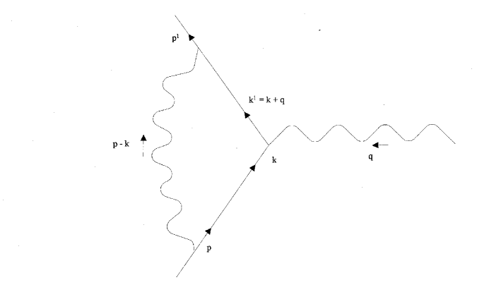
FIG. 1.: The electron vertex correction diagram. The wavy lines represent the massless vector boson propagator for the field $A_{\mu}$ which is directly related to the graviton field.

REFERENCES

- [1] R. R. Sastry, quant-ph/9903025.
- [2] R. R. Sastry, hep-th/9903171.
- [3] R. R. Sastry, hep-th/9903179.
- Isham ‘ [75] C.J. Isham, Quantum Gravity, eds. C.J. Isham, R. Penrose, D.W. Sciama, Clarendon Press, 1975.
- Isham ‘ [81] C.J. Isham, Quantum Gravity 2, eds. C.J. Isham, R. Penrose, D.W. Sciama, Clarendon Press, 1981.
- Hawking ‘ [78] S.W. Hawking, in Recent Developments in Gravitation Cargese Lectures, eds. M. Levy & S. Deser, Plenum, 1978.
- Weinberg ‘ [89] S. Weinberg, Rev. Mod. Phys. 61, 1 (1989).
- Goldhaber ’ [74] A. Goldhaber & M. Nieto, Phys. Rev. D9, 119 (1974).
- Hawking ‘ [84] S.W. Hawking, Phys. Lett. 134B, 403-404 (1984).
- Wald ‘ [84] R.M. Wald, General Relativity, The University of Chicago Press, 1984.
- Peskin ‘ [95] M.E. Peskin & D.V. Schroeder, Introductory Quantum Field Theory, Addison-Wesley, 1995.