USC-FT-7/99

hep-th/9905057

CHERN-SIMONS GAUGE THEORY: TEN YEARS AFTER

J. M. F. Labastida

Departamento de Física de Partículas
Universidade de Santiago de Compostela
E-15706 Santiago de Compostela, Spain
e-mail: labasti@fpaxp1.usc.es

A brief review on the progress made in the study of Chern-Simons gauge theory since its relation to knot theory was discovered ten years ago is presented. Emphasis is made on the analysis of the perturbative study of the theory and its connection to the theory of Vassiliev invariants. It is described how the study of the quantum field theory for three different gauge fixings leads to three different representations for Vassiliev invariants. Two of these gauge fixings lead to well known representations: the covariant Landau gauge corresponds to the configuration space integrals while the non-covariant light-cone gauge to the Kontsevich integral. The progress made in the analysis of the third gauge fixing, the non-covariant temporal gauge, is described in detail. In this case one obtains combinatorial expressions, instead of integral ones, for Vassiliev invariants. The approach based on this last gauge fixing seems very promising to obtain a full combinatorial formula. We collect the combinatorial expressions for all the Vassiliev invariants up to order four which have been obtained in this approach.

1 Introduction

The connection between Chern-Simons gauge theory and the theory of knot and link invariants was established by Edward Witten ten years ago [2]. Since then the theory has been studied from a variety of points of view. Many of the standard methods in field theory have been applied, generating results which became important in the development of knot theory. The interplay between quantum field theory and knot theory has been very rich in both directions. Though the results have been more spectacular in the knot theory direction, one must not forget that the developments in Chern-Simons gauge theory have constituted a constant test of our knowledge in quantum field theory. In fact, it has been found that not always the quantum field theory methods have been able to provide the right answer. As it will be described in detail, the work of the last few years reveals that there are some issues which are not yet understood when dealing with non-covariant gauges.

The term Chern-Simons theory appears in different contexts of quantum field theory. In this conference these words have been heard at least in half of the talks. It is therefore convenient to specify which type of Chern-Simons gauge theory I will be dealing with in this paper. I will refer by the term Chern-Simons gauge theory to a quantum field theory in three-dimensions whose action is the integral on a smooth compact boundaryless three-manifold of a Chern-Simons form associated to a semi-simple non-abelian gauge group. This theory was originally considered by several authors [3], but only after the work by Witten its connection with the theory of knot and link invariants was discovered. This occurred in the summer of 1988. Some of the other theories also named by the term Chern-Simons have been recently reviewed in [4].

The presentation contained in this paper will not follow a chronological order. The development of the theory of knot and link invariants from a mathematical point of view in the last fifteen years have been very impressive and at some stages it has developed parallel to Chern-Simons gauge theory. I will try to make a correspondence from each side for each of the topics treated. Though I have witnessed the development of Chern-Simons gauge theory in detail during these ten years, I might have missed some of the corresponding achievements from the mathematical side. I apologize in advance if some omission in this respect takes place. The order in the presentation is chosen in such a way that the progress made in these ten years can be understood starting from the basics of both, knot and Chern-Simons gauge theory. At each stage the results obtained in the context of Chern-Simons gauge theory are interpreted in the context of knot theory from a mathematical point of view.

The study of Chern-Simons gauge theory is an unusual one because it was first analyzed from a non-perturbative point of view. The original paper by Witten presents a series of non-perturbative methods which led him to show that the vacuum expectation values (vevs) of the relevant operators of the theory are polynomial invariants like the Jones polynomial [5] and its generalization. Other non-perturbative analysis were made one year later and soon some of the first perturbative studies started to appear. However, only some years later, after the advent of Vassiliev invariants [6, 7], the importance of the study of the perturbative series expansion was recognized. From a field theory point of view this lack of interest was understandable. Usually, field theorist can grasp only some of the perturbative aspects of their theories. Since in Chern-Simons gauge theory we had a good handle on its exact solution, why should one care about its perturbative series? It turned out that the coefficients of the perturbative series are important invariants. Their study applying perturbation theory led to interesting expressions for them. The invariance of these coefficients was clear from the beginning. What was not obvious is that they were invariants with a very special feature, they were Vassiliev invariants or invariants of finite type. Though this was known since the work by Bar-Natan [8] and Birman and Lin [9] in 1993, its proof in a quantum field theory context had to wait until 1997 [10].

Once the importance of the perturbative series expansion was realized several works addressed its study. Again the richness inherent to quantum field theory become a powerful tool and the form of this series expansion was studied for different gauge-fixings. The pioneer perturbative calculations in the covariant Landau gauge [11, 12] were later extended and analyzed from a general point of view [13, 14]. All these works constituted part of the inspiration for the formulation by Bott and Taubes of their configuration space integral [15]. Their integral corresponds precisely to the perturbative series expansion of the vev of a Wilson loop in Chern-Simons gauge theory in the Landau gauge. Before the work by Bott and Taubes, Kontsevich presented a different integral [16] for Vassiliev invariants. This integral turned out to correspond to the perturbative series expansion of the vev of a Wilson loop in the non-covariant light-cone gauge [17, 18, 19]. The interplay between physics and mathematics was very fruitful in these developments. This is rather clear in the case of the covariant Landau gauge. In the case of the light-cone gauge, the Chern-Simons counterpart took place much later than the formulation of the Kontsevich integral. However, as stated in the paper by Kontsevich, some of his insight to write down his integral originated from Chern-Simons gauge theory. A very recent work [20] shows from a mathematical point of view that both, the Kontsevich integral and the Bott and Taubes configuration space integral lead to the same invariants. From a field theory point of view this is just a consequence of the gauge invariance of the theory.

Gauge invariance is a powerful tool: it allows to study the theory for different gauge fixings. In the last few years a new gauge fixing has been considered: the non-covariant temporal gauge [17, 21]. This gauge has the important feature that the integrals which are present in the expressions for the coefficients of the perturbative series expansion can be carried out, leading to combinatorial expressions [21]. This has been shown to be the case up to order four and it seems likely that the approach can be generalized. In this analysis a crucial role is played by the factorization theorem for Chern-Simons gauge theory proved in [22]. The resulting expressions are better presented when written in terms of Gauss diagrams for knots [23]. Some recent results from the mathematical side seem to indicate the existence of a combinatorial formula of this type [24]. At present Chern-Simons gauge theory is the only approach which have provided combinatorial expressions for all the Vassiliev invariants up to order four. Work is in progress from both sides to obtain a general combinatorial expression. Hopefully, a coherent interplay between them will provide the widely searched general combinatorial expression for Vassiliev invariants.

The paper is organized using the following table as a guide. I have listed on the left hand side the mathematical counterparts of the topics of Chern-Simons gauge theory listed on the right hand side.

Knot Theory	Chern-Simons Gauge Theory
Knots and links	Wilson loops
Knot and link polynomial invariants	Vevs of products of Wilson loops
Singular knots	Operators for singular knots
Invariants for singular knots	Vevs of the new operators
Finite type or Vassiliev invariants	Coeffs. of the perturbative series
Chord diagram	First coeff. of the perturbative series
{1T,4T} and {1T,AS,IHX,STU}	Lie-algebra structure of group factors
Configuration space integral	Landau gauge
Kontsevich integral	Light-cone gauge
??	Temporal gauge

The sections of the paper will deal with the development of these topics from the point of view of Chern-Simons gauge theory, indicating the basic details from its knot theory counterpart. Notice that the entry in the knot-theory column corresponding to the temporal gauge has not been filled in yet.

The paper is organized as follows. In sect. 2, Chern-Simons gauge theory is introduced, as well as the basics of the theory of knots and links. A brief summary of some of the results obtained in the context of non-perturbative Chern-Simons gauge theory is also included in this section. In sect. 3, singular knots are introduced and their corresponding operators are defined. These operators are studied and their connection to chord diagrams is discussed. In sect. 4, Chern-Simons gauge theory is studied from a perturbative point of view. Using the covariant Landau gauge the coefficients of the perturbative series expansion are analyzed, obtaining configuration space integrals. In sect. 5, the perturbative series expansion is reobtained in the non-covariant light-cone gauge. The resulting series is the same as the Kontsevich integral for Vassiliev invariants. In sect. 6, the perturbative series expansion is analyzed in a different non-covariant gauge, the temporal gauge. The general procedure to obtain combinatorial expressions for Vassiliev invariants is presented and their explicit form is given for all the primitive invariants up to order four. Finally, in sect. 7, some concluding remarks are presented. Two tables list all the primitive Vassiliev invariants up to order four for all prime knots up to nine crossings.

2 Knots, links and Wilson loops

Let us begin recalling the basic elements of Chern-Simons gauge theory. This theory is a quantum field theory whose action is based on the Chern-Simons form associated to a non-abelian gauge group. The fundamental data in Chern-Simons gauge theory are the following: a smooth three-manifold $M$ which will be taken to be compact, a gauge group $G$, which will be taken semi-simple and compact, and an integer parameter $k$. The action of the theory is the integral of the Chern-Simons form associated to a gauge connection $A$ corresponding to a gauge group $G$:

$$S_{{\scriptstyle{\rm CS}}}(A)={k\over 4\pi}\int_{M}{\hbox{\rm Tr}}(A\wedge dA+\frac{2}{3}A\wedge A\wedge A).$$ (2.1)

In this expression the trace is taken in the fundamental representation of the gauge group. The action possesses the following behavior under gauge transformations,

$$A \rightarrow A+g^{-1}dg,$$ (2.2)

$$S_{{\scriptstyle{\rm CS}}}(A) \rightarrow S_{{\scriptstyle{\rm CS}}}(A)-4\pi yk\omega(g),$$ (2.3)

where $g$ is a map $g:M\rightarrow G$, $\omega(g)$ is its winding number,

$$\omega(g)={1\over 48\pi^{2}y}\int_{M}{\hbox{\rm Tr}}(g^{-1}dg\wedge g^{-1}dg\wedge g^{-1}dg),$$ (2.4)

and $y$ the Dynkin index of the fundamental representation of $G$. Since the winding number (2.4) is an integer and $y$ is a half-integer, it follows that, for integer $k$, the exponential,

$$\exp(iS_{{\scriptstyle{\rm CS}}}(A)),$$ (2.5)

which is the quantity that enters in the computation of vevs, is invariant under gauge transformations.

A theory characterized by an action like (2.1), which is independent of the metric on the three-manifold $M$, is a topological quantum field theory. In this theory, appropriate observables lead to vevs which correspond to topological invariants. Candidates to be observables of this type have to satisfy two properties. On the one hand they must be metric independent, on the other hand they must be gauge invariant. Wilson loops verify these two properties and they are therefore the paramount observables to be considered in Chern-Simons gauge theory.

Wilson loop operators correspond to the holonomy of the gauge connection $A$ along a loop. Given a representation $R$ of the gauge group $G$ and a 1-cycle $\gamma$ on $M$, it is defined as:

$$W_{\gamma}^{R}(A)={\hbox{\rm Tr}}_{R}\big{(}{\hbox{\rm Hol}}_{\gamma}(A)\big{)}={\hbox{\rm Tr}}_{R}{\hbox{\rm P}}\exp\int_{\gamma}A.$$ (2.6)

Products of these operators are the natural candidates to obtain topological invariants after computing their vev. These vevs are formally written as:

$$\langle W_{\gamma_{1}}^{R_{1}}W_{\gamma_{2}}^{R_{2}}\cdots W_{\gamma_{n}}^{R_{n}}\rangle\\ =\int[DA]W_{\gamma_{1}}^{R_{1}}(A)W_{\gamma_{2}}^{R_{2}}(A)\cdots W_{\gamma_{n}}^{R_{n}}(A){\hbox{\rm e}}^{iS_{{\scriptscriptstyle{\rm CS}}}(A)},$$

where $\gamma_{1}$, $\gamma_{2}$,$\dots$,$\gamma_{n}$ are 1-cycles on $M$ and $R_{1}$, $R_{2}$ and $R_{n}$ are representations of $G$. In (2), the quantity $[DA]$ denotes the functional integral measure and it is assumed that an integration over connections modulo gauge transformations is carried out. As usual in quantum field theory this integration is not well defined. Field theorists have elaborated a variety of methods to go around this problem and provide some meaning to the right hand side of (2). These methods fall into two categories, perturbative and non-perturbative ones, and their degree of success mostly depends on the quantum field theory under consideration. Fortunately, in Chern-Simons gauge theory these methods have been very fruitful. Indeed, in the pioneer work by Witten in 1988 he showed, using non-perturbative methods, that when one considers non-intersecting cycles $\gamma_{1}$, $\gamma_{2}$,$\dots$,$\gamma_{n}$ without self-intersections, the vevs (2) lead to the polynomial invariants discovered a few years before starting with the work by V. F. Jones [5]. But before making a precise statement on what was achieved by Witten in [2] let us go through our first mathematical detour and collect some basic facts on knot theory.

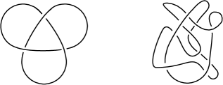
Figure 1: Two regular projections of the trefoil knot.

Knot theory studies embeddings $\gamma:$ $S^{1}\rightarrow M$. Two of these embeddings are considered equivalent if the image of one of them can be deformed into the image of the other by an homeomorphism on $M$. The main goal of the theory is to classify the resulting equivalence classes. Each of these classes is a knot. Most of the study in knot theory has been carried out for the simple case $M=S^{3}$. This is the situation which has been widely studied from a Chern-Simons theory point of view. Chern-Simons gauge theory, however, being a formulation intrinsically three-dimensional, provides a framework to study the case of more general three-manifolds $M$. In this respect, Chern-Simons gauge theory seems more promising than other approaches whose formulation possesses a two-dimensional flavor.

A powerful approach to classify knots is based on the construction of knot invariants. These are quantities which can be computed taking a representative of a class and are invariant within the class, i.e., are invariant under continuous deformations of the representative chosen. At present, it is not known if there exist enough knot invariants to classify knots. Vassiliev invariants are the most promising candidates but is already known that if they do classify, infinitely many of them are needed.

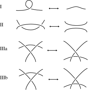
Figure 2: Reidemeister moves.

The problem of the classification of knots in $S^{3}$ can be reformulated in a two-dimensional framework using regular knot projections. Given a representative of a knot in $S^{3}$, deform it continuously in such a way that the projection on a plane has simple crossings. Draw the projection on the plane and at each crossing use the convention that the line that goes under the crossing is erased in a neighborhood of the crossing. The resulting diagram is a set of segments on the plane, containing the relevant information at the crossings. Two diagrams corresponding to two regular knot projections of the trefoil knot are shown in fig. 1. A given knot might have many regular projections. The first question to ask is if one can define an equivalence relation among regular projections whose equivalence classes coincide with the equivalence classes of knots. Reidemeister answered this question in the affirmative many years ago. He proved that the problem of classifying knots was equivalent to the problem of classifying knot projections modulo a series of relations among them. These relations, known as Reidemeister moves, are the ones shown in fig. 2. Invariance of a quantity under the three Reidemeister moves is called invariance under ambient isotopy. If a quantity is invariant under all but the first is said to possess invariance under regular isotopy. It is instructive to find out the way that the Reidemeister moves can be applied to the two diagrams shown in fig. 1 to show that, indeed, they are equivalent.

The formalism described for knots generalizes to the case of links. For a link of $n$ components one considers $n$ embeddings, $\gamma_{i}:$ $S^{1}\rightarrow M$, $i=1,\dots,n$, with no intersections among them. Again, the main problem that link theory faces is the problem of their classification modulo homeomorphisms on $M$. In this case one can also define regular projections and reformulate the problem in terms of their classification modulo the Reidemeister moves shown in fig. 2. Notice that $n=1$ is just the case which corresponds to knots.

The study of knot and link invariants experimented important progress in the eighties. In 1984 V. F. Jones [5] discovered a new invariant which strongly influenced the field. He formulated the celebrated Jones polynomial, an invariant which was able to distinguish many more knots and links that previous knot invariants. To have a flavor of the type of quantities one is dealing with, let us describe it in some detail.

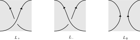
Figure 3: Links which enter in the skein rule of the Jones polynomial.

The Jones polynomial can be defined very simply in terms of skein relations. These are a set of rules that can be applied to the diagram of a regular knot projection to construct the polynomial invariant. They establish a relation between the invariants associated to three links which only differ in a region as shown in fig. 3. Notice that arrows have been provided to each of the segments entering fig. 3. Indeed, the Jones polynomial as well as, in general, the rest of polynomial invariants which will be discussed below are defined for oriented links. Thus, an arrow must be introduced for each of the components of a link. Though polynomial knot invariants are invariant under a reversal of its orientation, link polynomial invariants are not.

If one denotes by $V_{L}(t)$ the Jones polynomial corresponding to a link $L$, being $t$ the argument of the polynomial, it must satisfy the skein relation:

$${1\over t}V_{L_{+}}-tV_{L_{-}}=(\sqrt{t}-{1\over\sqrt{t}})V_{L_{0}},$$ (2.7)

where $L_{+}$, $L_{-}$ and $L_{0}$ are the links pictured in fig. 3. This relation plus a choice of normalization for the unknot ($U$) are enough to compute the Jones polynomial for any link. The standard choice for the unknot is:

$$V_{U}=1,$$ (2.8)

though it is not the most natural one from the point of view of Chern-Simons gauge theory. For the trefoil knot shown in fig. 1 this polynomial is: $V_{T}=t+t^{3}-t^{4}$. Notice that actually $V_{L}(t)$, in general, is not a polynomial. First, it might contain negative powers of $t$. Indeed, for the mirror image of the trefoil knot shown in fig. 1, $\tilde{T}$, one easily finds that $V_{\tilde{T}}=t^{-1}+t^{-3}-t^{-4}$. Actually this is just an example of a general feature of the Jones polynomial that under a reversal of the orientation of the ambient space $S^{3}$ it behaves as $V_{\tilde{L}}(t)=V_{L}(t^{-1})$, a property which makes it stronger than the Alexander polynomial which was not able two discriminate among links $L$ and $\tilde{L}$ which are mirror images of each other. Second, $V_{L}(t)$ might contain a factor of the form $\sqrt{t}$. This is always the case if $L$ has an even number of components. For example, for the simplest two-component link, the Hopf link, it takes the form: $V_{H}=\sqrt{t}(1+t^{2})$.

After Jones work in 1984, many other polynomial invariants where discovered. Two of the most celebrated ones are the HOMFLY [25] and the Kauffman [26] polynomial invariants. The first one possesses a skein rule with three entries similar to the one in fig. 3 and can be computed in the same way. The novelty is that it is a polynomial in two variables. The second one is also a polynomial in two variables but its corresponding skein rule is not as simple as in the Jones or HOMFLY polynomials. In general, the generalizations involve skein rules containing more than three terms and the computation of invariants becomes more complicated. Often other methods have to be used. Before entering in the discussion of the general framework which accounts for all these developments let us turn back to Chern-Simons gauge theory.

The pioneer work by Witten in 1988 showed that the vevs of products of Wilson loops (2) correspond to the Jones polynomial when one considers $SU(2)$ as gauge group and all the Wilson loops entering in the vev are taken in the fundamental representation $F$. For example, if one considers a knot $K$, Witten showed that,

$$V_{K}(t)=\langle W_{K}^{F}\rangle,$$ (2.9)

provided that one performs the identification:

$$t=\exp({2\pi i\over k+h}),$$ (2.10)

where $h=2$ is the dual Coxeter number of the gauge group $SU(2)$. Witten also showed that if instead of $SU(2)$ one considers $SU(N)$ and the Wilson loop carries the fundamental representation, the resulting invariant is the HOMFLY polynomial. The second variable of this polynomial originates in this context from the $N$ dependence. But these cases are just a sample of the general framework which Chern-Simons gauge theory offers. Taking other groups and other representations one possesses an enormous set of knot and link invariants. For some other special cases the resulting invariants correspond to specific polynomial invariants. For example, in one considers $SO(N)$ as gauge group and Wilson loops carrying the fundamental representation one is led to the Kauffman polynomial. If instead one considers $SU(2)$ as gauge group and the Wilson loops carry a representation of spin $j/2$ one rediscovers the Akutsu-Wadati [27] polynomials. Notice that the formalism allows to consider different representations for each of the components of a link, leading to the so-called colored polynomial invariants.

Chern-Simons gauge theory constitutes a framework where an enormous variety of knot and link invariants can be considered. The theory can be studied for arbitrary groups and arbitrary representations. But on top of this it also provides the basis to study these invariants in more general three-manifolds. In addition, Chern-Simons gauge theory also allows to consider a more general set of observables called graphs [28] that certainly constitutes an important generalization which has not been much exploited from the field theory point of view.

The framework established from Chern-Simons gauge theory has been also formulated from a mathematical point of view. In general, the invariants inherent to Chern-Simons gauge theory have been reobtained and properly defined using contexts different than quantum field theory. This has been a very fruitful arena in the field of algebraic topology in the last ten years. There exist now a quantum group approach to polynomial invariants [29], and the general theory, including knots, links and graphs has been formulated at a categorical level [30].

A particular invariant of three-manifolds which deserves special attention is the partition function of Chern-Simons gauge theory. This quantity is hard to obtain from a field theory point of view. However, it has been properly defined from a mathematical point of view using triangulations of the three-manifold. The resulting invariant is known as the Witten-Reshetekhin-Turaev invariant [31], and it corresponds to the mentioned partition function. The partition function has been studied for some three-manifolds in [32]. The Witten-Reshetekhin-Turaev invariant can be obtained from Chern-Simons gauge theory using lattice gauge theory methods and placing the quantum field theory on a triangulated three-manifold [33]. Recently, new developments based in Chern-Simons gauge theory has led to new formulae for the partition function [34]. The approach seems very promising and it might lead to simpler computational methods for these invariants.

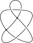
Figure 4: Regular projection of a singular knot with two double points.

Many non-perturbative studies of Chern-Simons gauge theory were performed in the years following Witten’s seminal work. The quantization of the theory was studied from the point of view of the operator formalism [35, 36, 37] and from more geometrical methods [38]. Also, its connection to two-dimensional conformal field theory was further elucidated [39] .A powerful method for the general computation of knot and link invariants was constructed by Kaul and collaborators [40]. Methods to compute graph invariants were also built [41]. All these works provided good setups for calculation purposes that in some situations were able to provide the answer to some open questions in knot theory. For example, general expressions for torus knots and torus links were obtained for a variety of situations using the operator formalism [42]. The problem of finding a polynomial invariant which discriminates between the two chiralities of the knots $9_{42}$ and $10_{71}$ was solved [43] using the methods developed by Kaul and collaborators. This approach was also used to show that polynomial invariants do not distinguish isotopically inequivalent mutant knots and links [44]. The connection between Chern-Simons gauge theory and rational conformal field theory was used to build knot and link invariants from any conformal field theory [45, 46]. Chern-Simons gauge theory has had also important applications in the loop-representation approach to canonical quantum gravity [47, 48]. Recently, graphs have also become very important in this context and it turns out that their associated Vassiliev invariants are related to physical states in the framework of canonical quantum gravity [49].

3 Singular knots and their operators

In this section the mathematical point of view will be discussed first. This will motivate the need to consider vevs of new operators associated to loops with self-intersections. We will describe how Chern-Simons gauge theory leads, using quantum field theory techniques, to the same results as its mathematical counterpart.

In 1990, V. A. Vassiliev [6] introduced a new point of view to study the problem of the classification of knots. Based on Arnold’s work on singularity theory he studied the space of all smooth maps of $S^{1}$ into $S^{3}$. This includes maps with various types of singularities which divide the space into chambers, each corresponding to a knot type. Using methods of spectral sequences to obtain combinatorial conditions, Vassiliev constructed families of new invariants to characterize these chambers.

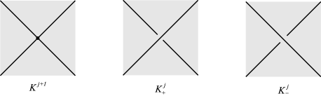
Figure 5: Regular projections which enter in the Vassiliev resolution of a double point.

Vassiliev approach was later reformulated by Birman and Lin [9] from an axiomatic point of view. As in the original formulation by Vassiliev [6], the starting point is based on the consideration of singular knots with $j$ double points. A representative of a singular knot with $j$ double points consists of the image of a map from $S^{1}$ into $S^{3}$ with $j$ simple self-intersections. Under homeomorphisms on $S^{3}$ these images form a class which constitute the singular knot itself. These singular knots can also be regularly projected. Fig. 4 shows one of these knots with two double points. The key ingredient in the construction by Birman and Lin is the observation that any knot invariant extends to generic singular knots by the Vassiliev resolution:

$$\nu({K^{j+1}})=\nu({K^{j}_{+}})-\nu({K^{j}_{-}}),$$ (3.1)

where $K^{j+1}$ is a singular knot with $j+1$ double points which differs from the knots $K^{j}_{+}$ and $K^{j}_{-}$ only in the region shown in fig. 5. Using this extension Birman and Lin characterized the invariants of finite type or Vassiliev invariants introducing the following definition:

A Vassiliev or finite type invariant of order $m$ is a knot invariant which is zero on the unknot and that, after extending it to singular knots, it is zero on singular knots $K^{j}$ with $j>m$ singular points, and different from zero on some $K^{m}$.

Vassiliev invariants form a vector space ${\cal V}$. Linear combinations of Vassiliev invariants are also Vassiliev invariants. Actually, to a Vassiliev invariant of order $m$ one can always add Vassiliev invariants of lower order obtaining additional Vassiliev invariants of order $m$. It is convenient to consider a filtration in the vector space of Vassiliev invariants using the order as grading. If one denotes by ${\cal V}_{m}$ the space of Vassiliev invariants of order $m$ one has the filtration,

$${\cal V}_{0}\subseteq{\cal V}_{1}\subseteq\cdots\subseteq{\cal V}_{m}\subseteq\cdots\subset{\cal V},$$ (3.2)

which leads to the graded vector space:

$${\rm gr}({\cal V})={\cal V}_{0}\oplus{\cal V}_{1}/{\cal V}_{0}\oplus{\cal V}_{2}/{\cal V}_{1}\oplus\cdots\oplus{\cal V}_{m+1}/{\cal V}_{m}\oplus\cdots$$ (3.3)

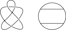
Figure 6: A singular knot and its corresponding chord diagram.

Besides introducing an axiomatic approach to Vassiliev invariants, Birman and Lin proved an important theorem in 1993 [9]. Let us consider any polynomial invariant $P_{K}(t)$ for a knot $K$. This polynomial could be any of the ones obtained from Chern-Simons gauge theory considering the vev of the corresponding Wilson loop for some group and some representation. Consider now the power series expansion:

$$Q_{K}(x)=P_{K}({\hbox{\rm e}}^{x})=\sum_{m=0}^{\infty}\nu_{m}(K)x^{m}.$$ (3.4)

Birman and Lin proved that if one extends the quantities $\nu_{m}(K)$ to Vassiliev invariants for singular knots using Vassiliev resolution (3.1), then $\nu_{m}(K)$ are Vassiliev invariants of order $m$. An immediate consequence of this theorem is that the coefficients of the perturbative expansion associated to the vev of a Wilson loop in Chern-Simons gauge theory are Vassiliev invariants. This property of the coefficients of the perturbative series expansion has been proved using standard quantum field theory methods [10]. Before describing how this has been achieved let us make some remarks on Vassiliev invariants and introduce one of them which is particularly important.

Once Vassiliev or finite type invariants have been introduced, there are two basic questions to ask. The first one is whether or not all the known numerical knot invariants are of finite type. The answer to this question is no. There are classical numerical knot invariants like the unknotting number, the genus or the crossing number which are not Vassiliev invariants. The second question is whether or not, in the case that Vassiliev invariants classify knots, one needs an infinite sequence of Vassiliev invariants to separate knots. This question has been answer in the affirmative.

From a singular knot with $m$ double points one can construct a particular object which determines Vassiliev invariants of order $m$: its chord diagram [8]. Given a singular knot $K^{m}$, its chord diagram, $CD(K^{m})$, is built in the following way. Take a base point and draw the preimages of the map associated to a given representative of $K^{m}$ on a circle. Then join by straight lines the pairs of preimages which correspond to each singular point. In fig. 6 the chord diagram corresponding to the singular knot of fig. 4 has been pictured. It is rather simple to observe that if $\nu(K^{m})$ is a Vassiliev invariant of order $m$ then it is completely determined by $CD(K^{m})$. Indeed, if one considers two singular knots with $m$ double points, $K^{m}_{1}$ and $K^{m}_{2}$, which differ in one crossing change then $CD(K^{m}_{1})=CD(K^{m}_{2})$. On the other hand, by Vassiliev resolution $\nu(K^{m}_{1})-\nu(K^{m}_{2})=\nu(K^{m+1})$. But $\nu(K^{m+1})=0$ and therefore all singular knots with $m$ double points leading to the same chord diagram have the same Vassiliev invariant of order $m$.

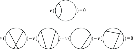
Figure 7: 1T and 4T relations among chord diagrams.

Chord diagrams play an important role in the theory of Vassiliev invariants. Since Vassiliev invariants of order $m$ for singular knots with $m$ double points are codified by chord diagrams one could ask if there are as many independent invariants of this kind as chord diagrams. The answer to this question is no. Chord diagrams are associated to knot diagrams and these diagrams must be considered modulo the equivalence relation dictated by the Reidemeister moves in fig. 2. These relations indeed impose some relations among chord diagrams, the so-called 1T and 4T relations [8]. They have been depicted in fig. 7.

Of particular importance is the space of chord diagrams modulo the 1T and 4T relations. This space is a graded space, graded by the number of chords:

$${\cal A} = \Big{\{}{\rm chord\,\,\,diagrams}\Big{\}}\,\,\Big{/}\,\,{\rm(1T,\,\,4T)}$$ (3.5)

$$= {\cal A}_{0}\oplus{\cal A}_{1}\oplus\cdots\oplus{\cal A}_{m}\oplus\cdots$$

Notice that ${\cal A}_{m}$ labels all the Vassiliev invariants of order $m$ for all knots with $m$ double points. The dimensions of the vector spaces ${\cal A}_{m}$ are not known in general. The space ${\cal A}$ possesses an algebraic structure that reduces the study of the spaces ${\cal A}_{m}$ to its connected part $\hat{\cal A}_{m}$. If $\hat{d}_{m}$ denotes the dimension of the connected part of ${\cal A}_{m}$, it is known that they take the following values up to order 12 [50]:

$m$	1	2	3	4	5	6	7	8	9	10	11	12
$\hat{d}_{m}$	0	1	1	2	3	5	8	12	18	27	39	55

The general expression for the dimensions of the spaces of chord diagrams $\hat{\cal A}_{m}$ is an open problem which has challenged many people. As it will be discussed below, these dimensions correspond in fact to the dimensions of the spaces of primitive Vassiliev invariants.

Figure 8: Diagram with one trivalent vertex.

The vector space of chord diagrams, ${\cal A}$, can be characterized in an equivalent way using trivalent diagrams an introducing a series of new relations. This characterization is very important because, as it will be shown below, it corresponds to the one that naturally arises from the point of view of Chern-Simons gauge theory. Let us expand the set of chord diagrams to a new set in which trivalent vertices are allowed. This means that now the lines in the interior of the circle can join a point on the circle to a point on one of the internal lines. Fig. 8 shows one of the new allowed diagrams. Notice that the point that looks like a four-valent vertex does not have any particular meaning. The new set of diagrams form a graded vector space whose grading is half the total number of vertices (internal trivalent vertices plus the previous vertices at the attachments of internal lines to the circle). Bar-Natan showed [8] that the previous space ${\cal A}$ in (3.5) is equivalent to the new one after modding out by the so-called 1T, AS, IHX and STU relations. The relation 1T is the previous one shown in fig. 7. The relation AS is the statement that the internal trivalent vertices are totally antisymmetric. Finally, the relations STU and IHX are the ones shown in fig. 9. Notice that in the relation STU the curved line corresponds to a piece of the circle of the diagram. The result proved by Bar-Natan in [8] is simply:

$${\cal A}=\Big{\{}{\rm trivalent\,\,\,diagrams}\Big{\}}\,\,\Big{/}\,\,{\rm(1T,\,\,AS,\,\,STU,\,\,IHX)}$$ (3.6)

where ${\cal A}$ is the space (3.5).

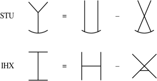
Figure 9: STU and IHX relations among trivalent diagrams.

The relations AS, STU and IHX are reminiscent of a Lie-algebra structure. If one assigns totally antisymmetric structure constants $f_{abc}$ to the internal trivalent vertices, and group generators $T_{a}$ to the vertices on the circle, the STU relation is just the defining Lie-algebra relation,

$$f_{abc}T_{c}=T_{a}T_{b}-T_{b}T_{a},$$ (3.7)

while the IHX relation corresponds to the Jacobi identity,

$$f_{abd}f_{dce}+f_{cad}f_{dbe}+f_{bcd}f_{dae}=0.$$ (3.8)

We will find out below that the group factors associated to the perturbative series expansion of the vev of a Wilson loop in Chern-Simons gauge theory correspond precisely to the space ${\cal A}$ in (3.5) or (3.6) in its representation in terms of trivalent graphs. In that context, the 1T relation is related to framing. In order to identify this group factors with the space ${\cal A}$ one must consider the perturbative series in a formal sense in which group factors are not particularized to a definite group. The group factors must be regarded as objects which simply satisfy relations (3.7) and (3.8) being $f_{abc}$ totally antisymmetric.

As follows from our discussion, singular knots play a central role in the theory of Vassiliev invariants. We must now ask about their role in Chern-Simons gauge theory. The first question to be addressed is about the natural operators that should be associated to them. Wilson loops are related to ordinary knots. What should be replacing the Wilson loop in the case of singular knots while maintaining Vassiliev resolution (3.1)? This question was answered in 1997 [10]. We will review here how these operators for singular knots are obtained using quantum field theory technics. The result will lead us to a proof of the theorem by Birman and Lin discussed above, and to make direct contact with chord diagrams.

We will begin studying the behavior of a difference of Wilson loops as the one that enters in Vassiliev resolution (3.1). Let us consider a family of smooth paths $\gamma_{u}$ parametrized by the continuous parameter $u$, such that for $u=0$ the path $\gamma_{0}$ possesses a self-intersection at some point $P$, i.e., for $u=0$ it has a double point. For $u>0$ ($u<0$) the path presents an overcrossing (undercrossing) near the point $P$. A family of paths with these features has been pictured in fig. 10. The path $\gamma_{0}(v)$ has a double point at $v=s_{1}$ and $v=t_{1}$ with $s_{1}<t_{1}$. Paths $\gamma_{u}(v)$ with $u\neq 0$ are different from $\gamma_{0}(v)$ only in the region in parameter space around $v=s_{1}$. The derivative of $\gamma_{u}(v)$ with respect to $u$ is only non-zero in that region. It vanishes away from $v=s_{1}$, in particular at $v=t_{1}$. In the two resolutions of a double point an overcrossing (undercrossing) corresponds to the one which leads to a crossing with positive (negative) sign, as depicted in fig. 11. Our goal is to study the first derivative of the vev of the Wilson loop $W_{\gamma_{u}}^{R}$ with respect to the parameter $u$. Due to the topological character of Chern-Simons gauge theory, one expects a step-function behaviour for $\langle W_{\gamma_{u}}^{R}\rangle$ as a function of $u$ in the neighborhood of $u=0$. This implies the presence of a delta function in its derivative. As shown below, this is in fact what one finds. Our goal is therefore to express

$$\langle W_{\gamma_{+}}^{R}\rangle-\langle W_{\gamma_{-}}^{R}\rangle=\int_{-\eta}^{\eta}du{d\over du}\langle W_{\gamma_{u}}^{R}\rangle,$$ (3.9)

where $\eta$ is some positive small real number, as the vev of some operator.

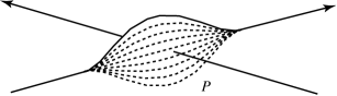
Figure 10: Family of paths with a intersection at the point $P$.

To compute the integrand on the right hand side of (3.9) we will use a series of well known properties of the Wilson loop and perform some formal manipulations in the integral functional inherent to vevs. Under a deformation of its path, the Wilson loop behaves as:

$${d\over du}W_{\gamma_{u}}^{R}=\oint dv\,\gamma_{u}^{{}^{\prime}\mu}(v)\dot{\gamma}_{u}^{\nu}(v)U_{\gamma_{u}}^{R}(s,v)F_{\mu\nu}(\gamma(v))U_{\gamma_{u}}^{R}(v,s),$$ (3.10)

where $U_{\gamma_{u}}^{R}(s,v)$ denotes a Wilson line which starts at $s$ and ends at $v$, and $F_{\mu\nu}$ is the curvature of the connection $A_{\mu}$. In (3.10) we have denoted derivatives with respect to the path parameter by a dot and derivatives with respect to $u$ by a prime. Recall that $\gamma_{u}^{{}^{\prime}}(v)$ is only different from zero in the region in parameter space around $v=s_{1}$. Another important property of the Wilson line is its behavior under a functional derivation with respect to the gauge connection:

$${\delta\over\delta A^{a}_{\mu}(x)}U_{\gamma_{u}}^{R}(s,t)=\int_{s}^{t}dw\,\dot{\gamma}_{u}^{\mu}(w)\delta^{(3)}(x,\gamma_{u}(w))U_{\gamma_{u}}^{R}(s,w)T^{a}U_{\gamma_{u}}^{R}(w,t).$$ (3.11)

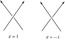
Figure 11: Signatures of an overcrossing and an undercrossing.

Relations (3.10) and (3.11) are common to any gauge theory. What makes Chern-Simons gauge theory special is that, after performing a variation of the action respect to the gauge connection one finds:

$${\delta\over\delta A_{\mu}^{a}(x)}S(A)={k\over 8\pi}\epsilon^{\mu\nu\rho}F_{\nu\rho}^{a}(x),$$ (3.12)

i.e., the field equation involves just the field strength $F_{\mu\nu}$ and not its derivative like in Yang-Mills theory.

Taking into account (3.10) and (3.12), and integrating by parts in connection space, one can write the integrand on the right hand side of (3.9) as:

$${d\over du}\langle W_{\gamma_{u}}^{R}\rangle={4\pi i\over k}\int[DA]{\hbox{\rm e}}^{iS(A)}\oint dv\,\epsilon_{\mu\nu\rho}\gamma_{u}^{{}^{\prime}\mu}(v)\dot{\gamma}_{u}^{\nu}(v){\delta\over\delta A_{\rho}^{a}(\gamma_{u}(v))}U_{\gamma_{u}}^{R}(s,v)T^{a}U_{\gamma_{u}}^{R}(v,t).$$ (3.13)

Using (3.11) and disregarding some subtle contributions related to framing [10] one finds:

$${d\over du}\langle W_{\gamma_{u}}^{R}\rangle={4\pi i\over k}\delta(u)\int[DA]{\hbox{\rm e}}^{iS(A)}{\hbox{\rm Tr}}\Big{[}T^{a}U_{\gamma_{u}}^{R}(s_{1},t_{1})T^{a}U_{\gamma_{u}}(t_{1},s_{1})\Big{]}.$$ (3.14)

As expected this expression involves a delta function in $u$. This proves in turn that for continuous deformations of the path which do not involve self-crossings the vev of a Wilson loop is invariant.

Using (3.9) and the result (3.14) one can read the operator which one must associate to a singular knot while maintaining Vassiliev resolution (3.1). Indeed, from (3.9) and (3.14) follows that

$${4\pi i\over k}{\Bigg{\langle}}{\hbox{\rm Tr}}\Big{[}T^{a}U_{\gamma}^{R}(s_{1},t_{1})T^{a}U_{\gamma}^{R}(t_{1},s_{1})\Big{]}{\Bigg{\rangle}}=\langle W_{\gamma_{+}}^{R}\rangle-\langle W_{\gamma_{-}}^{R}\rangle,$$ (3.15)

and therefore $(4\pi i/k){\hbox{\rm Tr}}\Big{[}T^{a}U_{\gamma}^{R}(s_{1},t_{1})T^{a}U_{\gamma}^{R}(t_{1},s_{1})\Big{]}$ is the sought operator. Notice that in (3.15) the subindex $u$ in the path has been suppressed. One can easily show that this operator is gauge invariant [10]. Its form is rather simple: split at the double point the Wilson loop into two Wilson lines and insert two group generators.

The result obtained for a single double point generalizes easily to deal with the general situation of $n$ double points. Let us consider a singular knot $K^{n}$ with $n$ double points, and let us assign to each double point $i$ a triple $\tau_{i}=\{s_{i},t_{i},T^{a_{i}}\}$ where $s_{i}$ and $t_{i}$, $s_{i}<t_{i}$, are the values of the $K^{n}$-parameter at the double point, and $T^{a_{i}}$ is a group generator. The gauge-invariant operator associated to the singular knot $K^{n}$ is:

$${\hskip-56.9055pt}({4\pi i\over k})^{n}{\hbox{\rm Tr}}\Big{[}T^{\phi(w_{1})}U(w_{1},w_{2})T^{\phi(w_{2})}U(w_{2},w_{3})T^{\phi(w_{3})}\cdots$$

$${\hskip 85.35826pt}\cdots U(w_{2n-1},w_{2n})T^{\phi(w_{2n})}U(w_{2n},w_{1})\Big{]},$$ (3.16)

where $\{w_{i};i=1,\dots,2n\}$, $w_{i}<w_{i+1}$, is the set that results from ordering the values $s_{i}$ and $t_{i}$, for $i=1,\dots,n$, and $\phi$ is a map that assigns to each $w_{i}$ the group generator in the triple to which it belongs.

The singular operators (3.16) lead to some immediate applications. First, it is easily shown that they constitute a proof of the theorem by Birman and Lin discussed above. This theorem was discussed at the beginning of this section. It states that if in any polynomial knot invariant with variable $t$ one substitutes $t\rightarrow{\hbox{\rm e}}^{x}$, and expand in powers of $x$, the coefficient of the power $x^{n}$ is a Vassiliev invariant of order $n$ (see eq. (3.4)). A Vassiliev invariant of order $n$ vanishes for all singular knots with $n+1$ crossings. In the language of Chern-Simons gauge theory the theorem by Birman and Lin can be rephrased, simply stating that the $n^{\rm th}$-order term of the perturbative series expansion of the vev of the Wilson loop associated to a given knot is a Vassiliev invariant of order $n$. We will now prove that this is so with the help of the operators (3.16).

The vevs of the operators (3.16) provide an invariant for a singular knot with $n$ double points. This singular-knot invariant can be expressed as a signed sum of $2^{n}$ invariants for non-singular knots. These $2^{n}$ invariants are the perturbative series expansion of the vev of the corresponding Wilson loops. To show that the coefficient of order $n$ of these vevs is a Vassiliev invariant or order $n$ is equivalent to proving that all the terms of order less than $n$ vanish in the signed sum. But the signed sum is precisely the vev of the operator (3.16). Since the perturbative series expansion of these operators starts at order $n$, the proof of the theorem by Birman and Lin follows.

With the help of the operators (3.16) one makes direct contact with chord diagrams. Let us consider the vevs of the operators (3.16) at order zero. Their expressions are simply obtained by setting $U=1$ in all the Wilson lines. Let us consider a singular knot $K^{n}$ with $n$ double points, $s_{i}$, $t_{i}$, with $s_{i}<t_{i}$, for $i=1,\dots,n$, in parameter space. As usual, with these data one constructs the triples: $\tau_{i}=\{s_{i},t_{i},T^{a_{i}}\}$. At lowest order in perturbation theory the operators (3.16) become the group factors,

$$v_{n}(K^{n})=({4\pi i\over k})^{n}{\hbox{\rm Tr}}\Big{[}T^{\phi(w_{1})}T^{\phi(w_{2})}T^{\phi(w_{3})}\cdots T^{\phi(w_{2n})}\Big{]},\\$$

where the set $\{w_{1},w_{2},\dots,w_{n}\}$, with $w_{j}<w_{j+1}$, is obtained by ordering the set $\{s_{i},t_{i};i=1,\dots,n\}$, and $\phi$ is the induced map that assigns to each $w_{j}$ the index of the group generator in the triple to which $w_{j}$ belongs. The indices entering (3) are paired. This allows the association, to each operator (3), of a diagram in which the $2n$ points are distributed on a circle and the ones that possess the same value of $\phi$ are joined by a line. The resulting diagrams are the chord diagrams for singular knots (as the one shown in fig. 6).

The quantities which result after the assignment of Lie-algebra data to chord diagrams are called weight systems [8]. For each system one chooses a group and a representation. As it will become clear in the next section, they correspond to the group theory factors in the context of Chern-Simons perturbation theory.

4 Vassiliev invariants and Chern-Simons perturbation theory

Vassiliev invariants of order $m$ for singular knots with $m$ double points have been studied in the previous section. From a mathematical point of view these are chord diagrams and from a Chern-Simons gauge theory point of view they are group factors or weight systems associated to chord diagrams. An important question that was addressed from the mathematical side some years ago was whether or not a weight system can be integrated to construct Vassiliev invariants for non-singular knots. The answer to this question turned to be affirmative. From the side of Chern-Simons gauge theory the positive answer to the question follows simply from the existence of the perturbative series expansion. In this section we will describe some of the basics of Chern-Simons perturbation theory. In the next section we will discuss the appearance of Vassiliev invariants from the integration of weight systems.

The perturbative study of Chern-Simons gauge theory started with the works by Guadagnini, Martellini and Mintchev [11] and by Bar-Natan [12]. These works dealt basically with the lowest non-trivial order in perturbation theory. To construct the perturbative series expansion of the vev of an operator when dealing with a gauge theory one is forced to make a gauge fixing. The first analysis of the Chern-Simons perturbation theory were made in the covariant Landau gauge. Subsequent studies [13, 14] in this gauge led to a framework linked to the theory of Vassiliev invariants, which culminated with the configuration space integral approach [15, 51]. In the rest of this section we will describe the structure of the perturbative series expansion of the vev of a Wilson loop in the covariant Landau gauge. Chern-Simons perturbation theory in this gauge for the case of more general three-manifolds has been considered in [52].

For a perturbative analysis it is more convenient to rescale the field entering the Chern-Simons action (2.1) in such a way that the coupling constant appears in the three-vertex of the theory. Rescaling the gauge field by

$$A_{\mu}\rightarrow gA_{\mu},$$ (4.1)

where $g=\sqrt{{4\pi\over k}}$, the Chern-Simons action (2.1) becomes,

$$S^{\prime}(A_{\mu})=\int{\hbox{\rm Tr}}(A\wedge dA+{2\over 3}gA\wedge A\wedge A).$$ (4.2)

This form of the action has the standard ${1\over 2}$ for the kinetic part since the trace of the fundamental representation is normalized as: ${\hbox{\rm Tr}}(T^{a}T^{b})={1\over 2}\delta^{ab}$. Notice that after the rescaling (4.1) covariant derivatives contain the coupling constant $g$.

As stated above, to construct the perturbative series a gauge fixing must be performed. We begin choosing a Lorentz gauge in which

$$\partial^{\mu}A_{\mu}=0.$$ (4.3)

The standard Faddeev-Popov construction leads us to consider the following gauge-fixed functional integral:

$$\int[DA_{\mu}DcD\bar{c}D\phi]{\hbox{\rm e}}^{iS^{\prime}(A_{\mu})+iS_{\scriptstyle{\rm gf}}(A_{\mu},c,\bar{c},\phi)},$$ (4.4)

where

$$S_{\scriptstyle{\rm gf}}(B_{\mu},c,\bar{c},\phi)=\int{\rm d}^{3}x{\hbox{\rm Tr}}(2\bar{c}\partial_{\mu}D^{\mu}c-2\phi\partial_{\mu}A^{\mu}-\lambda\phi^{2}).$$ (4.5)

In this action $\phi$ is a Lagrange multiplier which imposes the gauge condition, $c$ and $\bar{c}$ are anticommuting Faddeev-Popov ghosts, and $\lambda$ is a gauge-fixing parameter. The derivative in $D_{\mu}c$ is a covariant derivative. The functional integral in (4.4) must be done over all $A_{\mu}$ configurations and not only over gauge orbits. As a result of the gauge fixing, the exponent in (4.4) is invariant under the corresponding BRST transformations.

The field $\phi$ can be integrated out by performing a Gaussian integration in (4.4). One finds, up to an irrelevant multiplicative factor, that the functional integral (4.4) becomes:

$$\int[DA_{\mu}DcD\bar{c}]{\hbox{\rm e}}^{iI(A_{\mu},c,\bar{c})},$$ (4.6)

where

$$I(A_{\mu},c,\bar{c})=\int{\hbox{\rm Tr}}\big{[}\varepsilon^{\mu\nu\rho}(A_{\mu}\partial_{\nu}A_{\rho}+{2\over 3}gA_{\mu}A_{\nu}A_{\rho})-{1\over\lambda}A_{\mu}\partial^{\mu}\partial^{\nu}A_{\nu}+2\bar{c}\partial_{\mu}D^{\mu}c\big{]}.$$ (4.7)

In order to compute the vevs of operators involving Wilson loops like in (2) one must integrate these operators using (4.6). After expanding the path-ordered products in the Wilson loops one ends computing the functional integral over products of gauge fields. These are basically the correlation functions of the theory and are computed using standard quantum field theory methods, which lead to a set of computational rules called Feynman rules. These rules provide terms which are organized in even powers of $g$. They dictate that at order $g^{2m}$ two kinds of diagrams must be taken into account. The first group involves oriented trivalent graphs of the kind introduced in the previous section with $2m$ vertices and with the following assignments: for each internal line (gauge propagator),

$${i\over 4\pi}\delta_{ab}\epsilon^{\mu\nu\rho}{(x-y)_{\rho}\over|x-y|^{3}},$$ (4.8)

for each internal vertex,

$$-igf_{abc}\epsilon_{\mu\nu\rho}\int d^{3}x,$$ (4.9)

and for each vertex on the circle,

$$g(T^{a})_{i}^{j}.$$ (4.10)

The second set of diagrams involves propagators and vertices related to ghost fields. Contrary to gauge field propagators, dashed lines are used for ghost field propagators. The diagrams of the second set are also trivalent diagrams but they must contain at least one dashed line. Dashed lines can not be attached to the circle. They are always attached to internal lines via the ghost-gauge field-ghost trivalent vertex. We will not reproduce here the form of the ghost-related ingredients of the Feynman rules. We will describe, however, what is their effect.

In writing the quantities associated to the Feynman rules (4.8), (4.9) and (4.10) the limit $\lambda\rightarrow 0$ has been taken. This is known as the Landau gauge. It simplifies the calculations since in this case there are not infrared divergences.

After applying the Feynman rules one finds that the perturbative series contains divergent terms. Since the coupling constant $g$ is dimensionless, the theory is, however, renormalizable. Power counting analysis [54] shows that actually the theory is superrenormalible. To deal with the divergent terms, the theory must be regularized. One can use a variety of regularizations. For most of the regularizations which have been studied it turns out that the theory is in fact finite, i.e., after removing the cutoff introduced in the regularization the resulting expressions are finite. Of course, one is free to choose an arbitrary scheme using a finite renormalization. The value of $k$ would be different in each scheme if its fixed from some “standard data”. In other words, the value of $k$ in a given scheme should be determined stating, for example, that the value of the vev of the Wilson loop for the trefoil knot divided by the partition function is a fixed quantity. Then, though working in different schemes, the computations of vevs for any other knot would agree.

Many regularizations have ben studied in the last ten years. There is a particular subset of them [53, 54, 55, 56] that naturally leads to a scheme in which a shift in the coupling constant $k$ occurs. In these regularizations the higher-loop contributions to the two- and three-point functions add up to a shift in $k$ which is precisely the dual of the Coxeter number of the gauge group. This is rather remarkable because it is the same shift that appears in non-perturbative studies of Chern-Simons gauge theory in connection with its associated two-dimensional conformal field theory [2]. Why this is so is not still well understood.

In our perturbative analysis we are going to assume that higher-loop corrections to two- and three-point functions just account for the shift in $k$ and therefore we will not consider them in the expansion. We will deal with the rest of the diagrams. The scheme is chosen so that we do not make any finite renormalization. This scheme is as good as any other but is the best to compare perturbative results to non-perturbative ones. As we will discuss in the next sections, in non-covariant gauges we will make a choice in which there is no shift and then, to compare to non-perturbative calculations, we must make a finite renormalization.

Before writing the form of the full perturbative series we must deal with another important subtlety. If one computes the first order contribution to the perturbative series expansion of the vev of a Wilson loop one finds that the resulting quantity is not a topological invariant. In the gauge fixing of the theory we have introduced a metric dependence that could lead to quantities which are not topological. This first order contribution is just a manifestation of it. Fortunately, only in this term, and in its propagation in higher order contributions, topological invariance is lost. The rest of the perturbative series expansion is truly topological. Thus, although vevs are not topological invariant quantities they fail to be so in a controllable way. The non-topological terms factorize and multiply a term which is topological. In non-perturbative studies one finds a related problem which is the need of the introduction of a framing for the knot under consideration [2]. In other words, instead of knots one must consider framed knots, or knots with a normal vector field assigned which defines a framing characterized by an integer. This integer is the number of times that the normal vector field winds around the knot. A framing can also be introduced in the perturbative approach so that the perturbative result coincides with the non-perturbative one. Let us describe how this is done.

The first order contribution to the vev of a Wilson loop has the form:

$$g^{2}{\hbox{\rm Tr}}(T^{a}T^{b})\oint dx^{\mu}\int^{x}dy^{\nu}{i\over 4\pi}\delta_{ab}\epsilon^{\mu\nu\rho}{(x-y)_{\rho}\over|x-y|^{3}}$$ (4.11)

$$= g^{2}{1\over 2}{\hbox{\rm Tr}}(T^{a}T^{b})\oint dx^{\mu}\oint dy^{\nu}{i\over 4\pi}\delta_{ab}\epsilon^{\mu\nu\rho}{(x-y)_{\rho}\over|x-y|^{3}}.$$

This expression is finite but depends on the shape of the knot. Let us introduce a framing and, together with the original knot, a companion knot located at the end point of the normal vector which defines the framing. If one replaces one of the original paths entering (4.11) by the path associated to the companion knot (which will be denoted by a prime), one finds Gauss formula for the linking number:

$$g^{2}{1\over 2}{\hbox{\rm Tr}}(T^{a}T^{b})\oint dx^{\mu}\oint^{\prime}dy^{\nu}{i\over 4\pi}\delta_{ab}\epsilon^{\mu\nu\rho}{(x-y)_{\rho}\over|x-y|^{3}}=l.$$ (4.12)

In this expression $l$ is an integer that counts the number of times that the vector associated to the framing winds the knot. The kind of point splitting associated to the framing leads to a perturbative result that agrees with the non-perturbative analysis. Either if we introduce the framing or we leave a non-topological term we obtain a good perturbative series expansion. The corresponding term factorizes. Thus, to deal with one or the other is a matter of taste but, as in the case of the shift, agreement with the non-perturbative analysis induces the approach based on the framing. We will follow this choice. The term that factorizes has the form:

$$\exp\big{(}2\pi ilh_{R}\big{)},\,\,\,\,\,\,\,h_{R}={1\over k+g^{\vee}}{\hbox{\rm Tr}}_{R}(T^{a}T^{a}).$$ (4.13)

The quantity $h_{R}$ can be identified with the conformal weight for the representation $R$ of the associated conformal field theory. The Feynman diagrams that lead to the framing factor are those diagrams which contain isolated chords once a canonical basis from group factors has been chosen. Canonical basis play a prominent role in our discussion but before defining them let us first take a look at the general form of the perturbative series.

Once we have dealt with the issues regarding the shift and the framing we are in the position to analyze the perturbative series expansion of the vev of a Wilson loop. The Feynman rules (4.8), (4.9) and (4.10) allow to split the contributions to each order in two factors: a geometrical factor which includes all the space dependence, and a group factor which includes all the group theoretical dependence. The general form is:

$$\langle W^{R}_{K}\rangle=\hbox{\rm dim}\,R\sum_{i=0}^{\infty}\sum_{j=1}^{d_{i}}\alpha_{ij}(K)r_{ij}(R)x^{i},$$ (4.14)

where,

$$x={2\pi i\over k}=ig^{2}/2$$ (4.15)

is the expansion parameter, $\hbox{\rm dim}\,R$ is the dimension of the representation $R$, $\alpha_{0,1}=r_{0,1}=1$, and $d_{0}=1$. Notice that higher-loop corrections to the two- and three-point functions must not be included in (4.14) so this series should correspond to the non-perturbative result without the shift. The factors $\alpha_{ij}(K)$ and $r_{ij}(R)$ appearing at each order $i$ incorporate all the dependence dictated from the Feynman rules apart from the dependence on the coupling constant, which is contained in $x$. Of these two factors, in the $r_{ij}(R)$ all the group-theoretical dependence is collected. These are the group factors mentioned above. The rest is contained in the $\alpha_{ij}(K)$ or geometrical factors. They have the form of integrals over the Wilson loop corresponding to the knot $K$ of products of propagators, as dictated by the Feynman rules. The first index in $\alpha_{ij}(K)$ denotes the order in the expansion and the second index labels the different geometrical factors which can contribute at the given order. Similarly, $r_{ij}(R)$ stands for the independent group structures which appear at order $i$, which are also dictated by the Feynman rules. The object $d_{i}$ in (4.14) is the dimension of the space of invariants at a given order. In our approach denotes the number of independent group structures which appear at that order. Notice that while the geometrical factors $\alpha_{ij}(K)$ are knot dependent but group and representation independent, the group factors are group and representation dependent but knot independent.

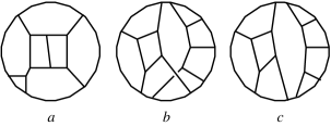
Figure 12: Examples of trivalent diagrams: a is connected while b and c are disconnected.

Among the basis of group factors which can be chosen in the perturbative series (4.14) there is a special class which turns out to be very useful. We will call it the class of canonical basis. Notice that to each group factor one can associate a trivalent diagram of the kind entering (3.6) if one considers the space of all semi-simple Lie groups (as that is the most general case for which the structure constants can be chosen totally antisymmetric). We will restrict to this case in what follows.

In order to introduce the concept of canonical basis we must first deal with a sort of classification of trivalent diagrams. A trivalent diagram will be called connected diagram if it is possible to go from one propagator (or internal line) to another without ever having to go through the external circle. The diagram will be called disconnected diagram if that is not possible. In this second case we say that the diagram has subdiagrams, which are the connected components of the whole diagram. Two subdiagrams are non-overlapping if we can move along the external circle meeting all the legs of one subdiagram first, and all the legs of the other second. By legs we mean internal lines attached to the external circle. If it is impossible to do that, the subdiagrams are overlapping. In fig. 12 the diagram a is connected while the diagrams b and c are disconnected. Of these last two, diagram b contains subdiagrams which are overlapping while c does not.

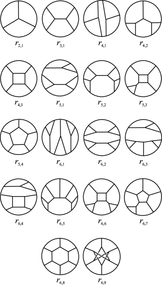
Figure 13: Choice of a canonical basis up to order 6.

In the expansion (4.14) there are many possible choices of independent groups factors $r_{ij}(R)$. Given all trivalent diagrams contributing to a given order in perturbation theory some of the resulting group factors might be related due to the Lie-algebra relations AS, STU and IHX as in (3.6). The group factors entering (4.14) are chosen to be associated to diagrams that constitute a basis. Its elements are the $r_{ij}(R)$ in (4.14). Of course, many choices are possible. In order to introduce our preferred choice let us first notice that due the STU relations one can always choose a basis such that the $r_{ij}(R)$ come from connected diagrams, or products of connected diagrams. That is, if there are subdiagrams, they can be chosen so that they do not overlap. The value of such an $r_{ij}(R)$ is the product of the values of its subdiagrams. This last statement follows from the fact that the part of the group factor associated to one of the subdiagrams is a diagonal matrix. Thus one can choose a basis built of connected trivalent diagrams and products of connected non-overlapping subdiagrams. A basis with this feature will be called a canonical basis. In fig. 13 a choice of canonical basis up to order six is shown.

We will denote by $r_{ij}^{c}(R)$ the group factors associated to a canonical basis, and $\alpha_{ij}^{c}(K)$ the corresponding geometrical factors. It was shown in [22] that then the perturbative series expansion (4.14) can be written as:

$$\langle W^{R}_{K}\rangle=\hbox{\rm dim}\,R\,\exp\left\{\sum_{i=1}^{\infty}\sum_{j=1}^{\hat{d}_{i}}\alpha_{ij}^{c}(K)\,r_{ij}^{c}(R)\,x^{i}\right\},$$ (4.16)

where $\hat{d}_{i}$ stands for the number of connected elements in the canonical basis at order $i$. Notice that $\alpha_{ij}^{c}(K)$ do not correspond uniquely to connected Feynman diagrams. The result (4.16) is known as the factorization theorem. Actually, it holds for arbitrary gauges, not only in the covariant Landau gauge as one could conclude from our discussion. The dimensions $\hat{d}_{i}$ are precisely the ones introduced for the connected part of the space of chord diagrams (3.5). Their values up to order 12 are the ones contained in the table shown after (3.5). The geometrical factors $\alpha_{ij}^{c}(K)$ are a selected set of Vassiliev invariants. They are called primitive Vassiliev invariants. If they are known, the values of the whole set of Vassiliev invariants follow. These primitive Vassiliev invariants have been computed for general classes of knots as torus knots [42, 57] up to order six.

The contribution at first order in (4.16) is precisely the framing factor (4.13). Thus, the factorization theorem (4.16) shows also its factorization. The rest of the terms in the exponent of (4.16) are knot invariants. The series contained in that exponent was analyzed by Bott and Taubes [15] in their work on the configuration space for Vassiliev invariants. They showed that the integral expression entering the geometrical factors $\alpha_{ij}^{c}(K)$ are convergent [15, 51]. Further work on the subject has led to a proof of their invariance [14, 58].

The explicit expression for the integrals entering in the second order contribution was first presented in [11]. It was later analyzed in detail by Bar-Natan [12]. It takes the form:

$$\alpha_{21}^{c}(K) = \frac{1}{4}\oint dx^{\mu}\int^{x}dy^{\nu}\int^{y}dz^{\rho}\int^{z}dw^{\sigma}\Delta_{\mu\rho}(x-z)\Delta_{\nu\sigma}(y-w)$$ (4.17)

$$- \frac{1}{16}\oint dx^{\mu}\int^{x}dy^{\nu}\int^{y}dz^{\rho}\int d^{3}\omega\,v_{\mu\nu\rho}(x,y,z;\omega),$$

where,

$$\Delta_{\mu\nu}(x-y)=\frac{1}{\pi}\epsilon_{\mu\rho\nu}\frac{(x-y)^{\rho}}{|x-y|^{3}},$$ (4.18)

and,

$$v_{\mu\nu\rho}(x,y,z;\omega)=\Delta_{\mu\sigma_{1}}(x-\omega)\Delta_{\nu\sigma_{2}}(y-\omega)\Delta_{\rho\sigma_{3}}(z-\omega)\epsilon^{\sigma_{1}\sigma_{2}\sigma_{3}}.$$ (4.19)

This invariant turns out to be the total twist of the knot and coincides mod 2 with the Arf invariant. The integral expression for the order three invariant, $\alpha_{31}^{c}(K)$, associated to the group factor $r_{31}$ shown in fig. 13 was first presented in [13]. We reproduce it here for completeness:

$$\alpha_{31}^{c}(K) ={1\over 8}\oint\,{dx_{1}^{\mu_{1}}}\int^{x_{1}}\,{dx_{2}^{\mu_{2}}}\int^{x_{2}}\,{dx_{3}^{\mu_{3}}}\int^{x_{3}}\,{dx_{4}^{\mu_{4}}}\int^{x_{4}}\,{dx_{5}^{\mu_{5}}}\int^{x_{5}}\,{dx_{6}^{\mu_{6}}}$$

$$\big{[} \Delta_{\mu_{1}\mu_{4}}(x_{1}-x_{4})\Delta_{\mu_{2}\mu_{6}}(x_{2}-x_{6})\Delta_{\mu_{3}\mu_{5}}(x_{3}-x_{5})$$

$$+\Delta_{\mu_{1}\mu_{3}}(x_{1}-x_{3})\Delta_{\mu_{2}\mu_{5}}(x_{2}-x_{5})\Delta_{\mu_{4}\mu_{6}}(x_{4}-x_{6})$$

$$+\Delta_{\mu_{1}\mu_{5}}(x_{1}-x_{5})\Delta_{\mu_{2}\mu_{4}}(x_{2}-x_{4})\Delta_{\mu_{3}\mu_{6}}(x_{3}-x_{6})\big{]}$$

$$+{1\over 4} \oint\,{dx_{1}^{\mu_{1}}}\int^{x_{1}}\,{dx_{2}^{\mu_{2}}}\int^{x_{2}}\,{dx_{3}^{\mu_{3}}}\int^{x_{3}}\,{dx_{4}^{\mu_{4}}}\int^{x_{4}}\,{dx_{5}^{\mu_{5}}}\int^{x_{5}}\,{dx_{6}^{\mu_{6}}}$$

$$\big{[} \Delta_{\mu_{1}\mu_{4}}(x_{1}-x_{4})\Delta_{\mu_{2}\mu_{5}}(x_{2}-x_{5})\Delta_{\mu_{3}\mu_{6}}(x_{3}-x_{6})\big{]}$$

$$-{1\over 32} \oint\,{dx_{1}^{\mu_{1}}}\int^{x_{1}}\,{dx_{2}^{\mu_{2}}}\int^{x_{2}}\,{dx_{3}^{\mu_{3}}}\int^{x_{3}}\,{dx_{4}^{\mu_{4}}}\int^{x_{4}}\,{dx_{5}^{\mu_{5}}}\int d^{3}y$$ (4.20)

$$\big{[} \Delta_{\mu_{1}\nu_{1}}(x_{1}-y)\Delta_{\mu_{2}\mu_{5}}(x_{2}-x_{5})\Delta_{\mu_{3}\nu_{3}}(x_{3}-y)\Delta_{\mu_{4}\nu_{4}}(x_{4}-y)\epsilon^{\nu_{1}\nu_{3}\nu_{4}}$$

$$+\Delta_{\mu_{1}\mu_{3}}(x_{1}-x_{3})\Delta_{\mu_{2}\nu_{2}}(x_{2}-y)\Delta_{\mu_{4}\nu_{4}}(x_{4}-y)\Delta_{\mu_{5}\nu_{5}}(x_{5}-y)\epsilon^{\nu_{2}\nu_{4}\nu_{5}}$$

$$+\Delta_{\mu_{1}\nu_{1}}(x_{1}-y)\Delta_{\mu_{2}\mu_{4}}(x_{2}-x_{4})\Delta_{\mu_{3}\nu_{3}}(x_{3}-y)\Delta_{\mu_{5}\nu_{5}}(x_{5}-y)\epsilon^{\nu_{1}\nu_{3}\nu_{5}}$$

$$+\Delta_{\mu_{1}\nu_{1}}(x_{1}-y)\Delta_{\mu_{2}\nu_{2}}(x_{2}-y)\Delta_{\mu_{3}\mu_{5}}(x_{3}-x_{5})\Delta_{\mu_{4}\nu_{5}}(x_{4}-y)\epsilon^{\nu_{1}\nu_{2}\nu_{4}}$$

$$+\Delta_{\mu_{1}\mu_{4}}(x_{1}-x_{4})\Delta_{\mu_{2}\nu_{2}}(x_{2}-y)\Delta_{\mu_{3}\nu_{3}}(x_{3}-y)\Delta_{\mu_{5}\nu_{5}}(x_{5}-y)\epsilon^{\nu_{2}\nu_{3}\nu_{5}}\big{]}$$

$$+{1\over 128} \oint\,{dx_{1}^{\mu_{1}}}\int^{x_{1}}\,{dx_{2}^{\mu_{2}}}\int^{x_{2}}\,{dx_{3}^{\mu_{3}}}\int^{x_{3}}\,{dx_{4}^{\mu_{4}}}\int d^{3}y\int d^{3}z$$

$$\big{[} \Delta_{\mu_{1}\nu_{1}}(x_{1}-y)\Delta_{\mu_{2}\sigma_{2}}(x_{2}-z)\Delta_{\mu_{3}\sigma_{3}}(x_{3}-z)\Delta_{\mu_{4}\nu_{4}}(x_{4}-y)\Delta_{\alpha\beta}(y-z)\epsilon^{\nu_{1}\alpha\nu_{4}}\epsilon^{\sigma_{3}\beta\sigma_{2}}$$

$$+\Delta_{\mu_{1}\nu_{1}}(x_{1}-y)\Delta_{\mu_{2}\nu_{2}}(x_{2}-y)\Delta_{\mu_{3}\sigma_{3}}(x_{3}-z)\Delta_{\mu_{4}\sigma_{4}}(x_{4}-z)\Delta_{\alpha\beta}(y-z)\epsilon^{\nu_{2}\alpha\nu_{1}}\epsilon^{\sigma_{4}\beta\sigma_{3}}\big{]}$$

Properties of the primitive Vassiliev invariants $\alpha_{21}^{c}(K)$ and $\alpha_{31}^{c}(K)$ have been studied in [59]. In these works the integral expressions for $\alpha_{21}^{c}(K)$ and $\alpha_{31}^{c}(K)$ were studied in the flat-knot limit and combinatorial expressions of the kind that will be presented below from the study in the temporal gauge were obtained.

5 Light-cone gauge and the Kontsevich integral

In the previous section, the perturbative series expansion of the vev of a Wilson loop in the covariant Landau gauge has been analyzed. A similar analysis can be carried out for the operators associated to singular knots which were introduced in sect. 3. The lowest order contributions in such an expansion are the group factors corresponding to chord diagrams. These group factors form a weight system. Before the development of operators for singular knots the following question was raised: could weight systems on chord diagrams be integrated to obtain invariants for non-singular knots? Kontsevich answered this question affirmatively in 1993. He showed that a weight system on chord diagrams of order $m$ determines a unique Vassiliev invariant on non-singular knots.

Kontsevich theorem is constructive in the sense that it provides an explicit expression for the Vassiliev invariant for non-singular knots. This expression is known as the Kontsevich integral. We will provide its explicit form below, after deriving it from the quantum field theory side. In the context of Chern-Simons gauge theory Kontsevich theorem is contained in our construction of operators for singular knots. One should think of the first order contribution of the vev of a singular knot as the weight system, and of the full perturbative series for vevs of Wilson loops as the integration of the weight system. Thus, the perturbative series expansion of the vev of a Wilson loop should correspond to the Kontsevich integral. This does not seem to be the case as the configuration space integrals found in the previous section have a different form than the integrals contained in Kontsevich theorem. This fact poses a puzzle which, however, is solved very simply.

Gauge theories can be studied in different gauges. The analysis carried out in the previous sections dealt with the covariant Landau gauge but many others could have been used. It turns out that the perturbative series which results in the non-covariant light-cone gauge leads to the Kontsevich integral. To show this is the main goal of this section. Vevs of gauge invariant operators are independent of the gauge chosen and therefore the expressions obtained in the light-cone gauge should be equivalent to the ones obtained in any other gauge. In this sense the analysis of operators for singular knots in Chern-simons gauge theory constituted a general proof, or gauge independent proof, of Kontsevich theorem. The configuration space integrals of the previous section can equally be regarded as an integration of weight systems on chord diagrams. Actually, very recently, it has been shown from the mathematical side [20] that both series of integrals are equivalent. A ratification of the gauge independence of gauge invariant operators mentioned above.

In order to deal with non-covariant gauges let us introduce a unit constant vector $n$. The gauge-fixing conditions of axial type which we will discuss in this and in the next section correspond to the choice:

$$n^{\mu}A_{\mu}=0.$$ (5.1)

In the case of the light-cone gauge the unit vector $n$ satisfies the condition $n^{2}=0$. The gauge fixed action of the theory is built following the standard Faddeev-Popov construction which leads to a functional integral as in (4.4) where now:

$$S_{\scriptstyle{\rm gf}}(B_{\mu},c,\bar{c},\phi)=\int{\rm d}^{3}x{\hbox{\rm Tr}}(\phi n^{\mu}A_{\mu}+bn^{\mu}D_{\mu}c+\lambda\phi^{2}).$$ (5.2)

Again, $\phi$ is a Lagrange multiplier which imposes the gauge condition, $c$ and $\bar{c}$ are anticommuting Faddeev-Popov ghosts, and $\lambda$ is a gauge-fixing parameter.

The higher-loop analysis in axial-type gauges is a very delicate issue. It requires to take into consideration some specific prescription to regulate unphysical poles. Fortunately, this analysis has been done for the case of Chern-Simons gauge theory in [60]. In these works it is shown that a regulator can be chosen so that the effect of higher-loop contributions for two- and three-point functions is a shift of the parameter $k$ as the one discussed in the previous section in the covariant Landau gauge. Though strictly speaking this has been proved at one loop, it is believed that, as in the case of covariant gauges, it holds at any order in higher loops. We will assume that higher-loop contributions to the two- and the three-point functions account for the shift of the parameter $k$. Notice that the gauge condition (5.1) does not fix the gauge completely. One still has gauge invariance under gauge transformations in the direction normal to $n$. The presence of this residual gauge invariance is a source of problems which, as it will be discussed below, are not yet solved. Another study of light-cone perturbation theory can be found in [61].

We will work in the limit $\lambda\rightarrow 0$. The theory greatly simplifies in this case. The propagator for the gauge field in momentum space acquires the simple form:

$$\delta_{ab}{\lambda\over(np)^{2}}(p_{\mu}p_{\nu}-{i\over\lambda}(np)\epsilon_{\mu\nu\rho}n^{\rho})\rightarrow-i\epsilon_{\mu\nu\rho}{n^{\rho}\over np}\delta_{ab}.$$ (5.3)

This propagator is orthogonal to the $n$-direction. This implies that there is no coupling to the ghosts fields and, furthermore, that there is no gauge field self-coupling. Thus there is only a Feynman rule to be taken into account to compute the vevs of operators: the one associated to the gauge field propagator. The group factors that remain in this case correspond just to chord diagrams. The fact that in this gauge no group factors with trivalent vertices have to be taken into account is a quantum field theory ratification of Bar-Natan theorem among the equivalence of the two representations, (3.5) and (3.6), of the space ${\cal A}$.

Non-covariant gauges share the problem of the presence of unphysical poles in their propagators [62]. This is manifest in (5.3). Several prescriptions have been proposed to avoid these unphysical poles. Usually, a prescription is chosen so that some particular properties of the correlation functions are fulfilled. In the light-cone gauge there is a natural prescription which is motivated by the simple form that (5.3) takes in coordinate space after performing a Wick rotation. As it will be shown below, this prescription leads to Kontsevich integral.

In the light-cone gauge it is convenient to introduce light-cone coordinates. Let us choose the unit vector $n$ as $(0,1,-1)$. The new coordinates are:

$$x^{+}=x^{1}+x^{2},\,\,\,\,\,\,x^{-}=x^{1}-x^{2},$$ (5.4)

and the new light-cone components for the gauge connection become:

$$A_{+}=A_{1}+A_{2},\,\,\,\,\,\,A_{-}=A_{1}-A_{2}.$$ (5.5)

The form of the propagator (5.3) in coordinate space is more conveniently expressed after performing a Wick rotation to Euclidean space. A point in Euclidean space will be denoted as $(t,z)$, where $z=x^{1}+ix^{2}$. After introducing $A_{z}=A_{1}+iA_{2}$ and $A_{\bar{z}}=A_{1}-iA_{2}$ one finds that there exist a prescription to deal with the unphysical pole in (5.3) which leads to:

$$\langle A_{\bar{z}}^{a}(x)A_{m}^{b}(x^{\prime})\rangle = 0,$$

$$\langle A^{a}_{m}(x)A^{b}_{n}(x^{\prime})\rangle = \delta^{ab}\epsilon_{mn}{1\over 2\pi i}{\delta(t-t^{\prime})\over z-z^{\prime}},$$ (5.6)

with $m,n=\{0,z\}$, and $\epsilon_{mn}$ is antisymmetric with $\epsilon_{0z}=1$. This is the gauge-field propagator that we will use in our analysis of the perturbative expansion of the vev of a Wilson loop.

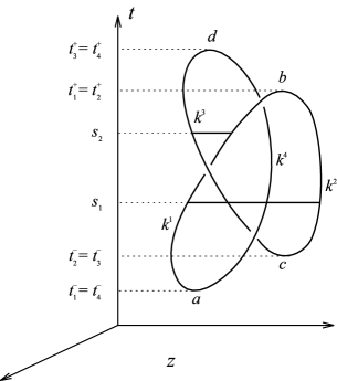
Figure 14: Example of a Morse knot.

Before entering into the analysis of the perturbative series expansion corresponding to the vev a Wilson loop, we must discuss the potential problems that might be encountered because of the particular form of the gauge-field propagator (5.6). This propagator is singular when its two end-points coincide. Actually, it is particularly singular in this situation because both the numerator and the denominator lead to divergences. In the light-cone gauge we have two special kinds of singularities, there may be situations in which only one, the numerator or the denominator, leads to a divergence. In order to avoid singularities from the numerator one is forced to avoid paths with sections in which $t$, the first component of a generic point $(t,z)$ is constant. This constraint implies that one must consider Morse knots. A Morse knot is a knot in which $t$ is a Morse function on it. A Morse knot is characterized by $2n$ extrema, half of them maxima, and the other half minima. An example of a Morse knot is depicted in fig. 14.

Another potential problem due to the structure of (5.6) comes from situations in which the two end-points of the propagator are close to one of the extrema of a Morse knot since the denominator then vanishes. To solve this problem one introduces a regularization procedure based on the introduction of a framing. The resulting invariants will correspond to invariants of framed knots. As in the case of the Landau gauge one finds [18] that a term like (4.13) factorizes. One is left then with a perturbative series expansion with group factors which correspond to chord diagrams without isolated chords. The ones with isolated chords just contribute to the framing factor.

In order to obtain the form of the perturbative series of the vev of a Wilson loop we begin by writing all the contributions at a given order $m$. To carry this out we must consider all possible ways of connecting $2m$ points on the Morse knot by $m$ propagators, taking into account the regularization described above, i.e., with one point of the propagator attached to $K$ and the other to its companion knot $K_{\varepsilon}$, and then path-order integrating. The path-order integration can be split into a sum such that in each term enters a path-ordered integration along $2m$ curves among the set $k^{i}$, $k^{i}_{\varepsilon}$, $i=1,\dots,2n$. This set of curves builds the Morse knot under consideration. A given term in this sum might contain propagators joining $k^{i}$ and $k^{i}_{\varepsilon}$. In this case one must introduce a factor $1/2$. The contributions coming from propagators joining $k^{i}$ and $k^{j}_{\varepsilon}$, with $i\neq j$, have also a factor $1/2$ since double counting occurs. Accordingly, propagators joining different curves must be replaced by $1/2$ the sum of their two possible choices of attaching their end-points.

Figure 15: Group factor at second order.

To each rearrangement of the $m$ propagators corresponds a group factor. These are easily obtained just using the rule (4.10). To fix ideas we will present in detail the second-order contribution, $m=2$, for a particular group factor, the one shown in fig. 15. This contribution is of the form

$$(ig)^{2}\int_{0}^{1}ds_{1}\int_{s_{1}}^{1}ds_{2}\int_{s_{2}}^{1}ds_{3}\int_{s_{3}}^{1}ds_{4}\dot{x}^{\mu_{1}}(s_{1})\dot{x}^{\mu_{2}}(s_{2})\dot{x}^{\mu_{3}}(s_{3})\dot{x}^{\mu_{4}}(s_{4})$$

$${\hskip-28.45274pt}\langle A_{\mu_{1}}^{a_{1}}\big{(}x(s_{1})\big{)}A_{\mu_{3}}^{a_{3}}\big{(}x(s_{3})\big{)}\rangle\langle A_{\mu_{2}}^{a_{2}}\big{(}x(s_{2})\big{)}A_{\mu_{4}}^{a_{4}}\big{(}x(s_{4})\big{)}\rangle{\hbox{\rm Tr}}(T^{a_{1}}T^{a_{2}}T^{a_{3}}T^{a_{4}}).$$ (5.7)

We will now write more explicitly one of the contributions to this multiple integral taking into account the form of the propagator (5.6). The delta function in this propagator imposes very strong restrictions on the possible contributions. Its presence implies that the only non-vanishing configurations are those in which the two end-points of each propagator are at the same height. To be more concrete let us consider the computation of (5.7) for the trefoil knot shown in fig. 14. This knot is made out of four curves, $k^{1}$, $k^{2}$, $k^{3}$ and $k^{4}$, whose end-points are the four critical points $a$, $b$, $c$ and $d$. The heights of these critical points are:

$$a \rightarrow t_{1}^{-}=t_{4}^{-},$$

$$b \rightarrow t_{1}^{+}=t_{2}^{+},$$

$$c \rightarrow t_{2}^{-}=t_{3}^{-},$$ (5.8)

$$d \rightarrow t_{3}^{+}=t_{4}^{+}.$$

They are depicted in fig. 14.

To obtain the contributions it is convenient to divide in four parts the circle that represents the knot in fig. 14 and join these parts by lines representing the propagators, taking into account the ordering of the four points to which they are attached. This ordering and the delta function in the height imply that no line can have its two end-points attached to the same part. They also imply that there are no contributions in which two end-points of different lines are attached to one part and the other two to another part. The contributions are easily depicted on the knot itself. One has been pictured in fig. 14. For each contribution, one must compute a sign, which takes into account the direction in which one travels along the knot in the new parametrization. To be more explicit, let us write, for example, the integral associated to the contribution shown in fig. 14. It takes the form:

$$(ig)^{2}{1\over(2\pi i)^{2}}{1\over{2^{2}}}\int_{t_{2}^{-}<s_{1}<s_{2}<t_{1}^{+}}ds_{1}ds_{2}$$

$${\hskip-48.36958pt}\Bigg{(}{\dot{z}_{1}(s_{1})-\dot{z}_{2}^{\prime}(s_{1})\over z_{1}(s_{1})-z_{2}^{\prime}(s_{1})}+{\dot{z}_{1}^{\prime}(s_{1})-\dot{z}_{2}(s_{1})\over z_{1}^{\prime}(s_{1})-z_{2}(s_{1})}\Bigg{)}\Bigg{(}{\dot{z}_{3}(s_{2})-\dot{z}_{1}^{\prime}(s_{2})\over z_{3}(s_{2})-z_{1}^{\prime}(s_{2})}+{\dot{z}_{3}^{\prime}(s_{2})-\dot{z}_{1}(s_{2})\over z_{3}^{\prime}(s_{2})-z_{1}(s_{2})}\Bigg{)},$$

(5.9)

where the primes denote the companion knot. The data entering this integral (5.9) are shown in fig. 14. Notice that this integral is not divergent if we take the limit $\varepsilon\rightarrow 0$ before performing the integration. This feature is common to all the contributions corresponding to the group factor under consideration. Only the contributions related to framing are potentially divergent. One could therefore remove in (5.9) the terms with primes and the factor $1/2^{2}$. The integral to be computed takes the form:

$$(ig)^{2}{1\over(2\pi i)^{2}}\int_{t_{2}^{-}<s_{1}<s_{2}<t_{1}^{+}}ds_{1}ds_{2}{\dot{z}_{1}(s_{1})-\dot{z}_{2}(s_{1})\over z_{1}(s_{1})-z_{2}(s_{1})}{\dot{z}_{3}(s_{2})-\dot{z}_{1}(s_{2})\over z_{3}(s_{2})-z_{1}(s_{2})}.$$ (5.10)

One of the two integrations can easily be performed, leading to:

$$(ig)^{2}{1\over(2\pi i)^{2}}\int_{t_{2}^{-}<s_{2}<t_{1}^{+}}ds_{2}\log\Bigg{(}{z_{1}(s_{2})-z_{2}(s_{2})\over z_{1}(t_{2}^{-})-z_{2}(t^{-}_{2})}\Bigg{)}{\dot{z}_{3}(s_{2})-\dot{z}_{1}(s_{2})\over z_{3}(s_{2})-z_{1}(s_{2})}.$$ (5.11)

Notice that, as argued before, this integral is finite. Although $z_{1}$ and $z_{2}$ get close to each other when $s_{2}\rightarrow t_{1}^{+}$, the singularity in the integrand, being logarithmic, is too mild to lead to a divergent result.

We are now in a position to write the form of the general contribution. Notice that the most significant fact of our previous discussion is the presence of the delta function in the height of the propagator (5.6). It implies that the only non-vanishing configurations of the propagators are those in which their two end-points have the same height; in other words, only contributions in which the line representing the propagator is horizontal do not vanish. This observation allows us to rearrange the contributions to the perturbative series expansion in the following way. Consider all possible pairings $\{z_{i}(s),z_{j}^{\prime}(s)\}$ of curves $k^{i}$ and $k^{j}_{\varepsilon}$, $i,j=1,\dots,2n$, where $2n$ is the number of extrema of the Morse knot under consideration. A contribution at order $m$ in perturbation theory will involve a path-ordered integral in the heights $s_{1}<\dots<s_{r}<\dots<s_{m}$ of a product of $m$ propagators:

$$\prod_{r=1}^{m}{dz_{i_{r}}(s_{r})-dz_{j_{r}}^{\prime}(s_{r})\over z_{i_{r}}(s_{r})-z_{j_{r}}^{\prime}(s_{r})}.$$ (5.12)

This product is characterized by a set of $m$ ordered pairings, each one labelled by a pair of numbers $(i_{r},j_{r})$ with $r=1,\dots,m$. We will denote an ordered pairing of $m$ propagators generically by $P_{m}$. One must take into account all possible ordered pairings, i.e., one must sum over all the possible $P_{m}$. The group factor that corresponds to each ordered pairing $P_{m}$ is simply obtained by placing the group generators at the end-points of the propagators and taking the trace of the product, which results after traveling along the knot. The resulting group factor will be denoted by $R(P_{m})$.

Another important fact that must be taken into account is the presence of a product of signs. For each pairing $P_{m}=\{(i_{r},j_{r}),r=1,\dots,m\}$ there will be a contribution from their product. Certainly, the result will be a sign that will depend on the ordered pairing $P_{m}$. We will denote such a product by $s(P_{m})$:

We are now in a position to write the full expression for the contribution to the perturbative series expansion at order $m$. It takes the form:

$$(ig^{2})^{m}\Big{(}{1\over 2\pi i}\Big{)}^{m}{1\over 2^{m}}\sum_{P_{m}}\int_{t_{P_{m}}^{-}<t_{1}<\dots<t_{r}<\dots<t_{m}<t_{P_{m}}^{+}}{\hskip-28.45274pt}s(P_{m})\prod_{r=1}^{m}{dz_{i_{r}}(t_{r})-dz_{j_{r}}^{\prime}(t_{r})\over z_{i_{r}}(t_{r})-z_{j_{r}}^{\prime}(t_{r})}R(P_{m}),$$ (5.13)

where $t_{P_{m}}^{+}$ and $t_{P_{m}}^{-}$ are highest and lowest heights, which can be reached by the last and first propagators of a given ordered pairing $P_{m}$. This expression corresponds to the Kontsevich integral for framed knots as presented in [63]. If one sets to zero all the group factors associated to diagrams with isolated chords one can disregard the primes in (5.13). We define $Z_{m}(K)$ as the resulting contribution at order $m$ divided by the dimension of the representation:

$$Z_{m}(K)={(ig^{2})^{m}\over{\rm dim}\,R}\Big{(}{1\over 2\pi i}\Big{)}^{m}{1\over 2^{m}}\sum_{P_{m}}\int_{t_{P_{m}}^{-}<t_{1}<\dots<t_{r}<\dots<t_{m}<t_{P_{m}}^{+}}{\hskip-28.45274pt}s(P_{m})\prod_{r=1}^{m}{dz_{i_{r}}(t_{r})-dz_{j_{r}}(t_{r})\over z_{i_{r}}(t_{r})-z_{j_{r}}(t_{r})}R(P_{m}),$$ (5.14)

This is the expression originally obtained by Kontsevich [16].

Figure 16: Unknot with four extrema.

It is well known that the Kontsevich integral is not a knot invariant. As first pointed out by Kontsevich himself [16], it has to be corrected by a subtle factor to have full invariance. Indeed, if the shape of a Morse knot is modified in such a way that the number of extrema changes, the Kontsevich integral (5.14) is not invariant. Kontsevich proposed the solution to this lack of invariance adding a factor now known as the Kontsevich factor. If we denote by $U$ the unknot with the shape shown in fig. 16, it turns out that the coefficients of the power expansion of:

$${1+\sum_{m=1}^{\infty}Z_{m}(K)\over(1+\sum_{m=1}^{\infty}Z_{m}(U))^{n\over 2}},$$ (5.15)

where $n$ denotes the number of extrema of the knot $K$, are truly Vassiliev invariants. The denominator of this expression is the so-called Kontsevich factor. It is not known how to obtain this factor using quantum field theory arguments. This is one of the open problems from the physical side. The study of gauge theories in non-covariant gauges presents many problems and, as it is the case here, in many occasions they lead to results which do not agree with their covariant-gauge counterparts. Often the cause for the discrepancy is linked to the ambiguity in the choice of a prescription to avoid non-physical poles. Most likely this is not the case at least for Chern-Simons gauge theory. As it is described in the next section, one finds that the Kontsevich factor is needed even if no specific prescription is taken. It is likely that the problem is related to the fact that there is a residual gauge invariance. As we discussed above, if one does not consider Morse knots, due to the residual gauge invariance, one gets divergent contributions. One needs to reduce to a single point all horizontal directions to avoid those divergences. Precisely when the number of points on the horizontal direction changes, i.e., when the knot is deformed so that the number of extrema gets modified one encounters the non-invariance of the Kontsevich integral (5.14). It is believed that a proper treatment of the residual gauge invariance will lead to understand the origin of the Kontsevich factor from a field theoretical point of view.

6 Temporal gauge and combinatorial formulae

The perturbative studies of Chern-Simons gauge theory that we have presented have led to two types of integral expressions for Vassiliev invariants. These expressions are not very useful from a computational point of view. Formulae of combinatorial type should be much preferred. There are some indications that a general combinatorial formula for Vassiliev invariants exists. On the one hand, the work on the study of the configuration space integrals in the limit of flat knots [59] originated a combinatorial expression for the Vassiliev invariant of order three. On the other hand, recent work from the mathematical side [64, 24] supports this conjecture. The search for the combinatorial formula led to the study of Chern-Simons gauge theory in the non-covariant temporal gauge [21]. This turns out to be the more suitable gauge to carry out all the intermediate integrals and obtain combinatorial expressions. No other approach has provided a combinatorial expression for the two primitive Vassiliev invariants at order four. The temporal gauge has been also treated in [17, 65].

The starting point of the analysis in the temporal gauge is the same as in the light-cone gauge. The gauge-fixing condition (5.1) is the same but now $n$ is a unit vector of the form $n^{\mu}=(1,0,0)$. The gauge-fixed action and the gauge-field propagator have also the same general form (5.2) and (5.3). As before, the propagator presents a pole at $np=0$, and a prescription to regulate it is needed. As observed in the previous sections, to construct the perturbative series expansion of the vev of a Wilson loop, we need the Fourier transform of (5.3). We will work in the limit $\lambda\rightarrow 0$. In the temporal gauge the momentum-space integral that has to be carried out has the form:

$$\Delta(x_{0},x_{1},x_{2})=\int_{M}{{\rm d}^{3}p\over(2\pi)^{3}}{{\hbox{\rm e}}^{i(p^{0}x_{0}+p^{1}x_{1}+p^{2}x_{2})}\over p^{0}}.$$ (6.1)

This integral is ill-defined due to the pole at $p^{0}=0$. To make sense of it a prescription has to be given to circumvent the pole. We will not take a precise prescription. Instead, we will work in a rather general framework. Let us first analyze the dependence of $\Delta(x_{0},x_{1},x_{2})$ in (6.1) on $x_{0}$. The pole in $p^{0}$ is avoided if, instead of (6.1), one analyses the derivative of $\Delta(x_{0},x_{1},x_{2})$ with respect to $x_{0}$. Considering $\Delta(x_{0},x_{1},x_{2})$ as a distribution one obtains:

$${\partial\Delta\over\partial x_{0}}=i\delta(x_{0})\delta(x_{1})\delta(x_{2}).$$ (6.2)

Integrating this expression with respect to $x_{0}$, one finds that any prescription would lead to a result of the following form:

$$\Delta(x_{0},x_{1},x_{2})={i\over 2}{\hbox{\rm sign}}(x_{0})\delta(x_{1})\delta(x_{2})+f(x_{1},x_{2}),$$ (6.3)

where $f(x_{1},x_{2})$ is a prescription-dependent distribution. The important consequence of the result (6.3) is that the dependence of $\Delta(x_{0},x_{1},x_{2})$ on $x_{0}$ has to be in the form ${\hbox{\rm sign}}(x_{0})\delta(x_{1})\delta(x_{2})$. This observation will be crucial in our analysis. We will actually work with the rather general formula (6.3) for $\Delta(x_{0},x_{1},x_{2})$. This form of the propagator will allow us to introduce the notion of kernels of a Vassiliev invariants and to design a procedure to compute combinatorial expressions for these invariants.

As for the issue of the framing and the shift, a similar analysis as the one in the light-cone gauge holds in this case. In the situation under consideration, however, it is more useful to consider a specific framing, the one in which the twist is zero or vertical framing. The linking number of a framed knot can be expressed as the sum of the writhe plus the twist associated to its regular projection. The writhe is the sum of the signatures of the crossings and the twist is the number of times that the framed knot, seen as a band, twists around its middle axis. Choosing a framing so that the twist is zero implies that the linking number coincides with the writhe. Thus a dependence on the writhe factorizes. This information turns out to be very useful in the analysis of the perturbative series.

We will review the salient facts of the analysis of the perturbative series expansion of the vev of a Wilson loop in the temporal gauge. the complete analysis can be found in [21]. Given a knot $K$ and one of its regular knot projections, ${\cal K}$, on the $x_{1},x_{2}$-plane which is a Morse knot in the $x_{1}$ and $x_{2}$ directions, the perturbative series expansion for the vev of the corresponding Wilson loop has the form:

$$\langle W_{K}^{R}\rangle=\langle W_{{\cal K}}^{R}\rangle_{{\rm temp}}\,\langle W_{U}^{R}\rangle^{b({\cal K})},$$ (6.4)

being,

$${1\over{\rm dim}\,R}\langle W_{K}^{R}\rangle=1+\sum_{i=1}^{\infty}v_{i}(K)x^{i},$$ (6.5)

and,

$${1\over{\rm dim}\,R}\langle W_{{\cal K}}^{R}\rangle_{{\rm temp}}=1+\sum_{i=1}^{\infty}\hat{v}_{i}({\cal K})x^{i}.$$ (6.6)

In these expressions $x$ denotes the coupling constant (4.15). The function $b({\cal K})$ is the exponent of the Kontsevich factor, which has been conjectured to be [21],

$$b({\cal K})={1\over 12}(n_{x_{1}}+n_{x_{2}}),$$ (6.7)

where $n_{x_{1}}$ and $n_{x_{2}}$ are the critical points of the regular projection ${\cal K}$ in both, the $x_{1}$ and the $x_{2}$ directions. In (6.4) $U$ denotes the unknot and $\langle W_{{\cal K}}^{R}\rangle_{{\rm temp}}$ is the vev of the Wilson loop corresponding to the regular projection ${\cal K}$ as computed perturbatively in the temporal gauge with the standard Feynman rules of the theory. Notice that though each of the factors on the right hand side of (6.4) depends on the regular projection chosen, the left hand side does not. While the coefficients $v_{i}(K)$ of the series (6.5) are Vassiliev invariants the coefficients $\hat{v}_{i}({\cal K})$ of (6.6) are not. The latter depend on the regular projection chosen.

An explicit combinatorial form (no integrals left) of the coefficients $\hat{v}_{i}({\cal K})$ in (6.6) would lead to a general combinatorial formula for Vassiliev invariants. Unfortunately, this has not been obtained yet at all orders. Only part of the contributions entering $\hat{v}_{i}({\cal K})$ have been explicitly written at all orders. These are the kernels introduced in [21]. The kernels are quantities which depend on the knot projection chosen and therefore are not knot invariants. However, at a given order $i$ a kernel differs from an invariant of type $i$ by terms that vanish in signed sums of order $i$. The kernel contains the part of a Vassiliev invariant which is the last in becoming zero when performing signed sums, in other words, a kernel vanishes in signed sums of order $i+1$ but does not in signed sums of order $i$. In some sense the kernel represents the most fundamental part of a Vassiliev invariant, i.e., the part that survives a maximum number of signed sums. Kernels plus the structure of the perturbative series expansion seem to contain enough information to reconstruct the full Vassiliev invariants. This was shown in [21] up to order four. The results obtained there will be presented below and rewritten in a more compact form. A summary of this approach has been presented in [23].

The expression for the kernels results after considering only the part of the propagator (6.3) which contains the sign function. This part involves a double delta function and therefore all the integrals can be performed. The result is a combinatorial expression in terms of crossing signatures after distributing propagators among all the crossings. Of course, the contribution from this part does not depend on the function $f(x_{1},x_{2})$ entering (6.3). The general expression can be written in a universal form much in the spirit of the universal form of the Kontsevich integral [16]. Let us consider a knot $K$ with a regular knot projection ${\cal K}$ containing $n$ crossings. Let us choose a base point on ${\cal K}$ and let us label the $n$ crossings by $1,2,\dots,n$ as we pass for first time through each of them when traveling along ${\cal K}$ starting at the base point. The universal expression for the kernel associated to ${\cal K}$ has the form:

$${\cal N}({\cal K})=\sum_{k=0}^{\infty}\Bigg{(}\sum_{m=1}^{k}\sum_{p_{1},\dots,p_{m}=1\atop p_{1}+\cdots+p_{m}=k}^{k}\sum_{i_{1},\dots,i_{m}=1\atop i_{1}<\cdots<i_{m}}^{n}{\varepsilon_{i_{1}}^{p_{1}}\cdots\varepsilon_{i_{m}}^{p_{m}}\over(p_{1}!\cdots p_{m}!)^{2}}\sum_{\sigma_{1},\dots,\sigma_{m}\atop\sigma_{1}\in P_{1},\dots,\sigma_{m}\in P_{m}}{\cal T}(i_{1},\sigma_{1};\dots;i_{m},\sigma_{m})\Bigg{)}.$$ (6.8)

In this equation $P_{m}$ denotes the permutation group of $p_{m}$ elements. The factors in the inner sum, ${\cal T}(i_{1},\sigma_{1};\dots;i_{m},\sigma_{m})$, are group factors which are computed in the following way: given a set of crossings, $i_{1},\dots,i_{m}$, and a set of permutations, $\sigma_{1},\dots,\sigma_{m}$, with $\sigma_{1}\in P_{1},\dots,\sigma_{m}\in P_{m}$, the corresponding group factor ${\cal T}(i_{1},\sigma_{1};\dots;i_{m},\sigma_{m})$ is the result of taking a trace over the product of group generators which is obtained after assigning $p_{1},\dots,p_{m}$ group generators to the crossings $i_{1},\dots,i_{m}$ respectively, and placing each set of group generators in the order which results after traveling along the knot starting from the base point. The first time that one encounters a crossing $i_{j}$ a product of $p_{j}$ group generators is introduced; the second time the product is similar, but with the indices rearranged according to the permutation $\sigma_{j}\in P_{j}$.

The universal formula (6.8) for the kernels can be written in a more useful way collecting all the coefficients multiplying a given group factor. Recall that the group factors can be labeled by chord diagrams. At order $k$ one has a term for each of the inequivalent chord diagrams with $k$ chords. Denoting chord diagrams by $D$, equation (6.8) can be written as:

$${\cal N}({\cal K})=\sum_{D}N_{D}({\cal K})D,$$ (6.9)

where the sum extends to all inequivalent chord diagrams. Our next task is to derive from (6.8) the general form of the kernels $N_{D}({\cal K})$. The concept of kernel can be extended to include singular knots by considering signed sums of (6.9), or, following [10], introducing vevs of the operators for singular knots. If ${\cal K}^{j}$ denotes a regular projection of a knot $K^{j}$ with $j$ simple singular crossings or double points, the corresponding universal form for the kernel possesses an expansion similar to (6.9):

$${\cal N}({\cal K}^{j})=\sum_{D}N_{D}({\cal K}^{j})D.$$ (6.10)

The general results about singular knots proved in [10] lead to two important features for (6.10). On the one hand, finite type implies that $N_{D}({\cal K}^{j})=0$ for chord diagrams $D$ with more than $j$ chords. On the other hand, $N_{D}({\cal K}^{j})=2^{j}\delta_{D,D({\cal K}^{j})}$, where $D({\cal K}^{j})$ is the chord diagram corresponding to the singular knot projection ${\cal K}^{j}$. As observed above, kernels constitute the part of a Vassiliev invariant which survives a maximum number of signed sums.

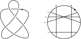
Figure 17: A regular knot projection and its corresponding Gauss diagram.

To compute $N_{D}({\cal K})$ we will introduce first the notion of the set of labeled chord subdiagrams of a given chord diagram. We will denote this set by $S_{D}$. This set is made out of a selected set of labeled chord diagrams that we now define. A labeled chord diagram of order $p$ is a chord diagram with $p$ chords and a set of positive integers $k_{1},k_{2},\dots,k_{p}$, which will be called labels, such that each chord has one of these integers attached. The set $S_{D}$ is made out of labeled chord diagrams which satisfy two conditions. These conditions are fixed by the form of the series entering the kernels (6.8). We will call the elements of $S_{D}$ labeled chord subdiagrams of the chord diagram $D$. They are defined as follows. A labeled chord subdiagram of a chord diagram $D$ with $k$ chords is a labeled chord diagram of order $p$ with labels $k_{1},k_{2},\dots,k_{p}$, $p\leq k$, such that the following two conditions are satisfied: a) $k_{1}+k_{2}+\cdots+k_{p}=k$; b) there exist elements $\sigma_{1}\in P_{k_{1}},\sigma_{2}\in P_{k_{2}},\dots,\sigma_{p}\in P_{k_{p}}$ of the permutation groups $P_{k_{1}},P_{k_{2}},\dots,P_{k_{p}}$ such that, after replacing the $j$-th chord diagram by $k_{j}$ chords arranged according to the permutation $\sigma_{j}$, for $j=1,\dots,p$, the resulting chord diagram is homeomorphic to $D$. The number of ways that permutations $\sigma_{1}\in P_{k_{1}},\sigma_{2}\in P_{k_{2}},\dots,\sigma_{p}\in P_{k_{p}}$ can be chosen is called the multiplicity of the labeled chord subdiagram. We will denote the multiplicity of a given labeled chord subdiagram, $s\in S_{D}$, by $m_{D}(s)$.

The chord diagram $D$ itself can be regarded as a labeled chord subdiagram such that its labels, or positive integers attached to its chords, are 1. It has multiplicity 1. All the elements of $S_{D}$ except $D$ have a number of chords smaller than the number of chords of $D$. Not all labeled chord diagrams are subdiagrams of $D$. However, given a labeled chord diagram with labels $k_{1},k_{2},\dots,k_{p}$ there can be different sets of permutations leading to $D$. The number of these different sets is the multiplicity introduced above. The elements of the sets $S_{D}$ for all chord diagrams $D$ up to order four which do not have disconnected subdiagrams are the following:

$$\longrightarrow \hskip 8.5359pt\mbox{\leavevmode \hskip 15.0pt}\hbox{\hskip-11.38092pt},\mbox{\leavevmode \hskip 15.0pt} \longrightarrow \hskip 8.5359pt\mbox{\leavevmode \hskip 15.0pt}\hbox{\hskip-11.38092pt},\mbox{\leavevmode \hskip 15.0pt}\hbox{\hskip-11.38092pt},2\mbox{\leavevmode \hskip 15.0pt} \longrightarrow \hskip 8.5359pt\mbox{\leavevmode \hskip 15.0pt}\hbox{\hskip-11.38092pt},\mbox{\leavevmode \hskip 15.0pt}\hbox{\hskip-11.38092pt},\mbox{\leavevmode \hskip 15.0pt} \longrightarrow \hskip 8.5359pt\mbox{\leavevmode \hskip 15.0pt}\hbox{\hskip-11.38092pt},\mbox{\leavevmode \hskip 15.0pt}\hbox{\hskip-11.38092pt},\mbox{\leavevmode \hskip 15.0pt}\hbox{\hskip-11.38092pt},2\mbox{\leavevmode \hskip 15.0pt} \longrightarrow \hskip 8.5359pt\mbox{\leavevmode \hskip 15.0pt}\hbox{\hskip-11.38092pt},2\mbox{\leavevmode \hskip 15.0pt} \longrightarrow \hskip 8.5359pt\mbox{\leavevmode \hskip 15.0pt}\hbox{\hskip-11.38092pt},\mbox{\leavevmode \hskip 15.0pt}\hbox{\hskip-11.38092pt},2\mbox{\leavevmode \hskip 15.0pt}\hbox{\hskip-11.38092pt},4\mbox{\leavevmode \hskip 15.0pt} \longrightarrow \hskip 8.5359pt\mbox{\leavevmode \hskip 15.0pt}\hbox{\hskip-11.38092pt},\mbox{\leavevmode \hskip 15.0pt}\hbox{\hskip-11.38092pt},2\mbox{\leavevmode \hskip 15.0pt}\hbox{\hskip-11.38092pt},\mbox{\leavevmode \hskip 15.0pt} \longrightarrow \hskip 8.5359pt\mbox{\leavevmode \hskip 15.0pt}\hbox{\hskip-11.38092pt},\mbox{\leavevmode \hskip 15.0pt}\hbox{\hskip-11.38092pt},\mbox{\leavevmode \hskip 15.0pt}\hbox{\hskip-11.38092pt},2\mbox{\leavevmode \hskip 15.0pt}\hbox{\hskip-11.38092pt},2\mbox{\leavevmode \hskip 15.0pt}\hbox{\hskip-11.38092pt},3\mbox{\leavevmode \hskip 15.0pt} \longrightarrow \hskip 8.5359pt\mbox{\leavevmode \hskip 15.0pt}\hbox{\hskip-11.38092pt},\mbox{\leavevmode \hskip 15.0pt}\hbox{\hskip-11.38092pt},\mbox{\leavevmode \hskip 15.0pt}\hbox{\hskip-11.38092pt},\mbox{\leavevmode \hskip 15.0pt}\hbox{\hskip-11.38092pt},\mbox{\leavevmode \hskip 15.0pt}$$

The numbers accompanying each labeled chord subdiagram denote their multiplicity. When no number is attached to a chord of a labeled chord diagram it should be understood that the corresponding label is 1.

In order to write our final expression for the kernels we need to recall the notion of Gauss diagram. Given a regular projection ${\cal K}$ of a knot $K$ we can associate to it its Gauss diagram $G({\cal K})$. The regular projection ${\cal K}$ can be regarded as a generic immersion of a circle into the plane enhanced by information on the crossings. The Gauss diagram $G({\cal K})$ consists of a circle together with the preimages of each crossing of the immersion connected by a chord. Each chord is equipped with the sign of the signature of the corresponding crossing. An example of Gauss diagram has been pictured in fig. 17. Gauss diagrams are useful because they allow to keep track of the sums involving the crossings which enter in (6.8) in a very simple form. Let us consider a chord diagram $D$ and one of its labeled chord subdiagrams $s\in S_{D}$. Let us assume that $s$ has $p$ chords and labels $k_{1},k_{2},\cdots,k_{p}$. We define the product,

$$\langle s,G({\cal K})\rangle,$$ (6.12)

as the sum over all the embeddings of $s$ into $G({\cal K})$, each one weighted by a factor,

$${\varepsilon_{1}^{k_{1}}\varepsilon_{2}^{k_{2}}\cdots\varepsilon_{p}^{k_{p}}\over(k_{1}!k_{2}!\cdots k_{p}!)^{2}},$$ (6.13)

where $\varepsilon_{1},\varepsilon_{2},\dots,\varepsilon_{p}$ are the signatures of the chords of $G({\cal K})$ involved in the embedding. Using (6.12) the kernels $N_{D}({\cal K})$ entering (6.9) can be written as,

$$N_{D}({\cal K})=\sum_{s\in S_{D}}m_{D}(s)\langle s,G({\cal K})\rangle,$$ (6.14)

where $m_{D}(s)$ denotes the multiplicity of the labeled subdiagram $s\in S_{D}$ relative to the chord diagram $D$.

The product (6.12) possesses important properties. First, it is independent of the base point chosen for the regular projection ${\cal K}$ and, correspondingly, for the Gauss diagram $G({\cal K})$. Second, it is of finite type. This means that if $s$ has $j$ chords, the result of computing a signed sum of order higher than $j$ is zero. Recall that signed sums of order $k$ are used to define quantities associated to singular knot projections with $k$ double points, as the ones entering (6.9). A signed sum of order $k$ contains $2^{k}$ terms which correspond to the possible ways of resolving $k$ double points into overcrossings and undercrossings. Each one has a sign which corresponds to the product of the signatures of the crossings involved in the $k$ double points. If $s$ is a labeled chord diagram with $j$ chords and all its labels take value one, the order-$j$ signed sum is $2^{j}$ if the configuration of the singular projection with $j$ double points associated to such a sum corresponds to the chord diagram $s$; otherwise its value is zero. This fact leads to the result mentioned above stating that:

$$N_{D}({\cal K}^{j})=2^{j}\delta_{D,D({\cal K}^{j})},$$ (6.15)

where $D({\cal K}^{j})$ is the chord diagram corresponding to the singular knot projection associated to the signed sum. Of course, the product (6.12) vanishes if the number of chords of $s$ is bigger than the number of chords of the Gauss diagram $G({\cal K})$.

The products (6.12) can be regarded as quantities of finite type associated to Gauss diagrams $G$ whether or not these correspond to a regular projection of a knot. Gauss diagrams can be studied as abstract objects characterized by chord diagrams with signs assigned to their chords. It is clear that in such a general context the quantities $\langle s,G\rangle$, as defined in (6.12), are of finite type. In other words, if $s$ has $j$ chords and $G$ is an abstract Gauss diagram, the product $\langle s,G\rangle$ vanishes under signed sums of order higher than $j$. This observation leads to conjecture that the product (6.12) might play an interesting role in the theory of virtual knots [66, 24].

The terms $\langle s,G({\cal K})\rangle$ entering (6.14) are related to the quantities $\chi({\cal K})$ defined in [21]. It is straightforward to obtain the following relations:

$$\langle\mbox{\leavevmode \hskip 15.0pt}\hbox{\hskip-11.38092pt},G({\cal K})\rangle = {1\over(j!)^{2}}\chi_{1}({\cal K}),\hbox{\hskip 8.5359pt}j\hbox{\hskip 5.69046pt}\hbox{\rm odd,} \vbox{\vskip 25.6073pt}\langle\mbox{\leavevmode \hskip 15.0pt}\hbox{\hskip-11.38092pt},G({\cal K})\rangle = \chi_{2}^{A}({\cal K}), \vbox{\vskip 25.6073pt}\langle\mbox{\leavevmode \hskip 15.0pt}\hbox{\hskip-11.38092pt},G({\cal K})\rangle = {1\over 16}\chi_{2}^{C}({\cal K}), \vbox{\vskip 25.6073pt}\langle\mbox{\leavevmode \hskip 15.0pt}\hbox{\hskip-11.38092pt},G({\cal K})\rangle = \chi_{3}^{B}({\cal K}), \vbox{\vskip 25.6073pt}\langle\mbox{\leavevmode \hskip 15.0pt}\hbox{\hskip-11.38092pt},G({\cal K})\rangle = {1\over 4}\chi_{3}^{D}({\cal K}), \vbox{\vskip 25.6073pt}\langle\mbox{\leavevmode \hskip 15.0pt}\hbox{\hskip-11.38092pt},G({\cal K})\rangle = \chi_{4}^{A}({\cal K}), \vbox{\vskip 25.6073pt}\langle\mbox{\leavevmode \hskip 15.0pt}\hbox{\hskip-11.38092pt},G({\cal K})\rangle = \chi_{4}^{C}({\cal K}), \vbox{\vskip 25.6073pt}\langle\mbox{\leavevmode \hskip 15.0pt}\hbox{\hskip-11.38092pt},G({\cal K})\rangle = \chi_{4}^{E}({\cal K}),\vbox{\vskip 25.6073pt} \langle\mbox{\leavevmode \hskip 15.0pt}\hbox{\hskip-11.38092pt},G({\cal K})\rangle = {1\over(j!)^{2}}n({\cal K}),\hbox{\hskip 8.5359pt}j\hbox{\hskip 5.69046pt}\hbox{\rm even,} \vbox{\vskip 25.6073pt}\langle\mbox{\leavevmode \hskip 15.0pt}\hbox{\hskip-11.38092pt},G({\cal K})\rangle = {1\over 4}\chi_{2}^{B}({\cal K}), \vbox{\vskip 25.6073pt}\langle\mbox{\leavevmode \hskip 15.0pt}\hbox{\hskip-11.38092pt},G({\cal K})\rangle = \chi_{3}^{A}({\cal K}), \vbox{\vskip 25.6073pt}\langle\mbox{\leavevmode \hskip 15.0pt}\hbox{\hskip-11.38092pt},G({\cal K})\rangle = {1\over 4}\chi_{3}^{C}({\cal K}), \vbox{\vskip 25.6073pt}\langle\mbox{\leavevmode \hskip 15.0pt}\hbox{\hskip-11.38092pt},G({\cal K})\rangle = {1\over 4}\chi_{3}^{E}({\cal K}), \vbox{\vskip 25.6073pt}\langle\mbox{\leavevmode \hskip 15.0pt}\hbox{\hskip-11.38092pt},G({\cal K})\rangle = \chi_{4}^{B}({\cal K}), \vbox{\vskip 25.6073pt}\langle\mbox{\leavevmode \hskip 15.0pt}\hbox{\hskip-11.38092pt},G({\cal K})\rangle = \chi_{4}^{D}({\cal K}), \vbox{\vskip 25.6073pt}\langle\mbox{\leavevmode \hskip 15.0pt}\hbox{\hskip-11.38092pt},G({\cal K})\rangle = \chi_{4}^{F}({\cal K}).$$

Notice that in the second relation $n({\cal K})$ denotes the number of crossings of the regular projection ${\cal K}$. The rest of the quantities on the right hand side of (6) were defined in [21].

         

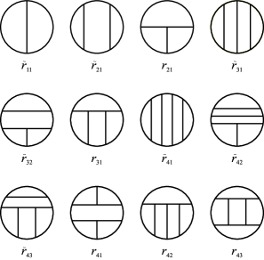
Figure 18: Choice of canonical basis up to order four which includes diagrams with isolated chords.

In [21], Vassiliev invariants up to order four were expressed in terms of these quantities and the crossing signatures. The strategy to obtain them was to start with the kernels (6.14) and exploit the properties of the perturbative series expansion of Chern-Simons gauge theory. A special role in the construction was played by the factorization theorem proved in [22]. In order to discuss some of the steps followed in [21] we will describe in detail the computation of the combinatorial expression for the Vassiliev invariant of order two. Let us begin considering a canonical basis for the group factors where diagrams with isolated chords are included. In fig. 18 this basis has been depicted up to order four. Tildes have been used to denote the diagrams with isolated chords. These diagrams are included because they provide useful information when working in the vertical framing. Instead of factorizing them out as in the previous sections, we will keep them in our analysis. In the analysis of the perturbative series it is important to know the expressions of all the chord diagrams in terms of the elements of the canonical basis in fig. 18. These expressions has been collected in figs. 19 and 20.

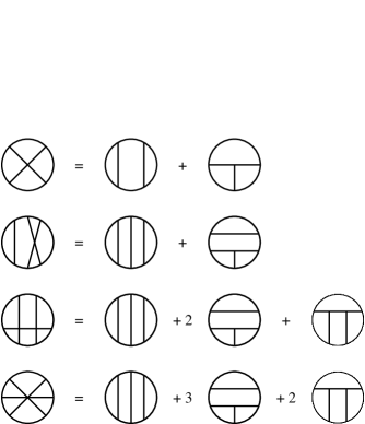
Figure 19: Expansion of chord diagrams in the canonical basis: orders two and three.

The perturbative series expansions entering (6.5) and (6.6) get some modifications relative to their form in (4.14). We will write them in the form:

$${1\over{\rm dim}\,R}\langle W_{{\cal K}}^{R}\rangle = 1+\sum_{i=1}^{\infty}\sum_{j=1}^{d_{i}}\alpha_{ij}(K)r_{ij}(R)x^{i}+\sum_{i=1}^{\infty}\sum_{j=1}^{\tilde{d}_{i}}\gamma_{ij}(K)\tilde{r}_{ij}(R)x^{i},$$

$${1\over{\rm dim}\,R}\langle W_{{\cal K}}^{R}\rangle_{{\rm temp}} = 1+\sum_{i=1}^{\infty}\sum_{j=1}^{d_{i}}\hat{\alpha}_{ij}({\cal K})r_{ij}(R)x^{i}+\sum_{i=1}^{\infty}\sum_{j=1}^{\tilde{d}_{i}}\hat{\gamma}_{ij}({\cal K})\tilde{r}_{ij}(R)x^{i}.$$

(6.17)

Notice that we have split the perturbative series into two sums. In the first sum the group factors, and their corresponding coefficients, are those appearing in (4.14), while in the second sum they are all the non-primitive elements coming from diagrams with isolated chords. The quantities $r_{ij}(R)$ and $\tilde{r}_{ij}(R)$ denote the respective group factors (whose corresponding chord diagrams up to order four are depicted in fig. 18), while $d_{i}$ and $\tilde{d}_{i}$ are the dimension of their basis at order $i$. As for the geometrical factors, $\alpha_{ij}(K)$ and $\gamma_{ij}(K)$ denote the Vassiliev invariants, primitive or not, we are looking for, while $\hat{\alpha}_{ij}({\cal K})$ and $\hat{\gamma}_{ij}({\cal K})$ are just the geometrical coefficients in the canonical basis of the perturbative Chern-Simons theory in the temporal gauge.

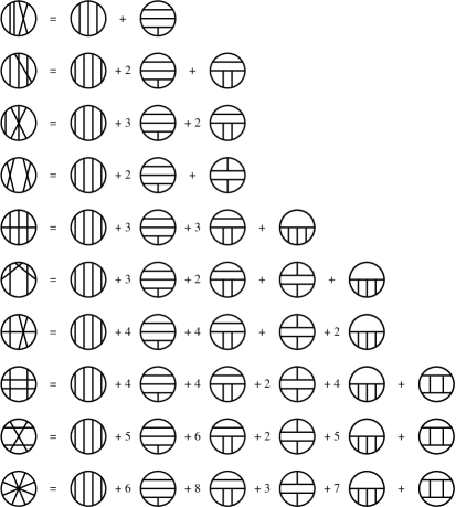
Figure 20: Expansion of chord diagrams in the canonical basis: order four.

The strategy is the following. First, the behavior of the unknown integrals entering $\hat{\alpha}_{ij}({\cal K})$ and $\hat{\gamma}_{ij}({\cal K})$ is analyzed; then the whole invariant is built, taking into account the corresponding global term as dictated by (6.4). Since, as shown in [22], the perturbative series expansion of the vev of the Wilson loop exponentiates in terms of the primitive basis elements, we have the following simple relation among primitives:

$$\alpha_{ij}(K)=\hat{\alpha}_{ij}({\cal K})+b({\cal K})\,\alpha_{ij}(U).$$ (6.18)

Let us begin with the analysis of $\hat{v}_{i}({\cal K})$ in (6.6). At first order we have no correction term (recall we are using the vertical framing), and the temporal gauge series provides the full regular invariant:

$$v_{1}(K)=\hat{v}_{1}({\cal K})=\Big{(}\hat{\gamma}_{11}^{E}({\cal K})+\hat{\gamma}_{11}^{D}({\cal K})\Big{)}\,\tilde{r}_{11}(R)$$ (6.19)

In this expression we have written the geometrical factor $\hat{\gamma}_{11}({\cal K})$ as a sum of two parts. The first one $\hat{\gamma}_{11}^{E}({\cal K})$ is built from the part of the propagator (6.3) not containing the unknown distribution $f$. The second one, $\hat{\gamma}_{11}^{D}({\cal K})$, depends on $f$. This type of decomposition can be done in general though at higher orders is more complicated. The integrals made out of the $f$-dependent part of the propagator (6.3) will be denoted by a superindex $D$ and a subindex which will label the chord diagram it comes from.

The general calculation requires a more subtle labelling. Given a chord diagram, each chord in it represents the propagator of the theory. Our propagator (6.3) contains two pieces: the explicit one, which leads to the signatures of the crossings, and the $f$-dependent one. The integrals arising from perturbation theory are a sum over all the possible ways of identifying the chords with each of them. So for a given diagram we will end up with different types of $D$ integrals, depending on how many $f$-terms they contain. When all the propagators in the integral are of this kind, it will be denoted simply by $D_{ij}$. If only one chord stands for the signature-dependent part, its evaluation will simply result in a crossing sign, $\varepsilon_{m}$, plus a restriction of the original integration domain. The chord standing for this factor is attached to the $m^{\rm th}$ crossing, which means that the ordered integration domain of the other chords of the $D$ integral is now limited by the position of that crossing. The resulting integral is written as:

$$\varepsilon_{m}\hat{\alpha}^{D_{m}}_{ij}\,,$$ (6.20)

with the subindex of $D$ denoting that one of the chords in the diagram is attached to the $m^{\rm th}$ crossing.

More involved cases arise when the integrand contains two signature-dependent terms of the propagator (6.3). In this case one must distinguish three subcases: both are attached to the same crossing, both are attached to different crossings and they have the pattern of the second case in fig. 21, and finally, both are attached to different crossings but this time they have the pattern of the third case in fig. 21. The set of pairs of crossings corresponding to the second case will be denoted by ${\cal C}_{a}$. The one corresponding to the third by ${\cal C}_{b}$. As only invariants up to order four will be considered, there is no need to handle the case where three or more signature-dependent terms of the propagator (but not all) are fixed to crossings. When the contribution does not contain $f$-dependent terms, the integral may be read from the kernels (6.8). It will be denoted by $\hat{\alpha}^{E}_{ij}$.

From the expression (6.8) for the kernels one easily finds, extracting the $k=1$ contribution:

$$\hat{\gamma}_{11}^{E}({\cal K})=\sum_{i=1}^{n}\varepsilon_{i},$$ (6.21)

where $n$ is the number of crossings in ${\cal K}$. This corresponds to the writhe, or linking number in the vertical framing, which is known to be the correct answer for $v_{1}(K)$. Thus we must have

$$\hat{\gamma}_{11}^{D}({\cal K})=0,$$ (6.22)

which agrees with our general arguments, showing that contributions with an odd number of $f$-dependent terms vanish.

At order two, the series expansion of (6.6) can be expressed as:

$$\hat{v}_{2}({\cal K})=\Big{(}\hat{\gamma}_{21}^{E}({\cal K})+\hat{\gamma}_{21}^{D}({\cal K})\Big{)}\,\tilde{r}_{21}(R)+\Big{(}\hat{\beta}_{21}^{E}({\cal K})+\hat{\beta}_{21}^{D}({\cal K})\Big{)}\,s_{21}(R),$$ (6.23)

where $s_{21}(R)$ is the group factor corresponding to the diagram on the left-hand side of the first row in fig. 19. We will denote by $s_{ij}$ group diagrams which appear at intermediate steps but do not belong to the chosen canonical basis of fig. 18. Their associated geometric factors will be denoted by $\beta_{ij}$. Notice that in (6.23) we have not included terms of the form $\sum\limits_{m=1}^{n}\varepsilon_{m}\alpha_{ij}^{D_{m}}$, since they have an odd number of $f$-dependent terms, and should not contribute. Terms of even order in the perturbative series expansion are invariant under a space reflection, while terms of odd order change sign. This implies that at even (odd) orders there are only contributions with an even (odd) number of $f$-dependent terms. In terms of the group factors of the chosen canonical basis (see fig. 18), the last expression, after using the first equation in fig. 19, takes the form:

$$\hat{v}_{2}({\cal K}) = \hat{\gamma}_{21}({\cal K})\,\tilde{r}_{21}(R)+\hat{\alpha}_{21}({\cal K})\,r_{21}(R)$$

$$= \Big{(}\hat{\gamma}_{21}^{E}({\cal K})+\hat{\beta}_{21}^{E}({\cal K})+\hat{\gamma}_{21}^{D}({\cal K})+\hat{\beta}_{21}^{D}({\cal K})\Big{)}\,\tilde{r}_{21}(R)+\Big{(}\hat{\beta}_{21}^{E}({\cal K})+\hat{\beta}_{21}^{D}({\cal K})\Big{)}\,r_{21}(R)$$

The computation of the two signature-dependent terms in (LABEL:ordtwob), $\hat{\gamma}_{21}^{E}$ and $\hat{\beta}_{21}^{E}$ is easily obtained from the kernels (6.8). One finds:

$$\hat{\gamma}_{21}^{E}=\langle\mbox{\leavevmode \hskip 15.0pt}\hbox{\hskip-11.38092pt}+\mbox{\leavevmode \hskip 15.0pt}\hbox{\hskip-11.38092pt},G({\cal K})\rangle$$ (6.25)

$$\hat{\beta}_{21}^{E}=\langle\mbox{\leavevmode \hskip 15.0pt}\hbox{\hskip-11.38092pt}+\mbox{\leavevmode \hskip 15.0pt}\hbox{\hskip-11.38092pt},G({\cal K})\rangle$$ (6.26)

Adding them up one obtains:

$$\hat{\gamma}_{21}^{E}+\hat{\beta}_{21}^{E}={1\over 2}\bigg{(}\sum_{i=1}^{n}\varepsilon_{i}\bigg{)}^{2}.$$ (6.27)

According to the factorization theorem [22] this is the whole non-primitive regular invariant of order two, $\gamma_{21}={1\over 2}(\sum\varepsilon_{i})^{2}$. Thus, we conclude that the order-two $D$-type terms must satisfy:

$$\hat{\gamma}_{21}^{D}+\hat{\beta}_{21}^{D}=0.$$ (6.28)

One more relation is needed to get rid of the two known quantities $\hat{\gamma}_{21}^{D}$ and $\hat{\beta}_{21}^{D}$. A new relation is obtained taking into account (6.18). One easily finds:

$$\alpha_{21}(K)=\langle\mbox{\leavevmode \hskip 15.0pt}\hbox{\hskip-11.38092pt}+\mbox{\leavevmode \hskip 15.0pt}\hbox{\hskip-11.38092pt},G({\cal K})\rangle+\hat{\beta}_{21}^{D}({\cal K})+b({\cal K})\,\alpha_{21}(U),$$ (6.29)

where $\alpha_{21}(U)$ stands for the value of this invariant for the unknot. The function $b({\cal K})$ is the unknown exponent in the global factor in (6.4). Using the fact that $\hat{\beta}_{21}^{D}({\cal K})$ and $b({\cal K})$ are equal in ${\cal K}$ and $\alpha({\cal K})$, being $\alpha({\cal K})$ the ascending diagram of ${\cal K}$, and that the latter is equivalent under ambient isotopy to the unknot, one finds:

$$\hat{\beta}_{21}^{D}({\cal K})=\alpha_{21}(U)\,[1-b({\cal K})]-\langle\mbox{\leavevmode \hskip 15.0pt}\hbox{\hskip-11.38092pt}+\mbox{\leavevmode \hskip 15.0pt}\hbox{\hskip-11.38092pt},G(\alpha({\cal K}))\rangle.$$ (6.30)

The final expression for the invariant is:

$$\alpha_{21}(K)=\alpha_{21}(U)+\langle\mbox{\leavevmode \hskip 15.0pt}\hbox{\hskip-11.38092pt},G({\cal K})\rangle-\langle\mbox{\leavevmode \hskip 15.0pt}\hbox{\hskip-11.38092pt},G(\alpha({\cal K}))\rangle,$$ (6.31)

where $\alpha_{21}(U)$ stands for the value of $\alpha_{21}$ for the unknot. Recall that the ascending diagram $\alpha({{\cal K}})$ of a knot projection ${\cal K}$ is defined as the diagram obtained by switching, when traveling along the knot from a base point, all the undercrossings to overcrossings. Ascending diagrams enter often in the combinatorial expressions and it is convenient introduce the following notation. A bar over a quantity $L({\cal K})$ indicates that the same quantity for the ascending diagram has to be subtracted, i.e.:

$$\bar{L}({\cal K})=L({\cal K})-L(\alpha({\cal K}))$$ (6.32)

where $\alpha({\cal K})$ denotes the standard ascending diagram of ${\cal K}$. Using this notation, the final form for the only primitive Vassiliev invariant at order two is:

$$\alpha_{21}(K)=\alpha_{21}(U)+\langle\mbox{\leavevmode \hskip 15.0pt}\hbox{\hskip-11.38092pt},\bar{G}({\cal K})\rangle.$$ (6.33)

The combinatorial expression (6.33) agrees with the formulae given in [59] and [67]. Notice that its dependence on $b({\cal K})$ has disappeared, so up to this order we do not get any condition on this function. The analysis at higher orders, however, imposes relations fro the function $b({\cal K})$. All the resulting relations are consistent with the ansatz (6.7). It is important to remark that the derivation of (6.33) that we have presented is much simpler than the one in the covariant gauge obtained in [59]. This simplicity is rooted in the special features of the temporal gauge that permits to have the compact expression (6.8) for the kernels, which are the essential building blocks of the combinatorial expressions for Vassiliev invariants.

The procedure followed at second order has been implemented in [21] for orders three and four. We will reproduce here the resulting combinatorial expressions. At order three there is only one primitive invariant. It takes the form:

$$\alpha_{31}(K)=\langle\mbox{\leavevmode \hskip 15.0pt}\hbox{\hskip-11.38092pt}+\mbox{\leavevmode \hskip 15.0pt}\hbox{\hskip-11.38092pt}+2\mbox{\leavevmode \hskip 15.0pt}\hbox{\hskip-11.38092pt},G({\cal K})\rangle-\sum_{i=1}^{n}\,\varepsilon_{i}({\cal K})\Big{[}\langle\mbox{\leavevmode \hskip 15.0pt}\hbox{\hskip-11.38092pt},G(\alpha({\cal K}))\rangle\Big{]}_{i}.$$ (6.34)

Several comments are in order to explain the quantities entering this expression. The sum is over all crossings $i$, $i=1,\dots,n$, and $\varepsilon_{i}({\cal K})$ denotes the corresponding signature. The square brackets $[$ $]_{i}$ enclosing a quantity $L({\cal K})$ denote:

$$\Big{[}L({\cal K})\Big{]}_{i}=L({\cal K})-L({\cal K}_{i_{+}})-L({\cal K}_{i_{-}}),$$ (6.35)

where the regular projection diagrams ${\cal K}_{i_{+}}$ and ${\cal K}_{i_{-}}$ are the ones which result after the splitting of ${\cal K}$ at the crossing point $i$ as shown in the first row of fig. 21. It is clear from the list (6) that these two invariants can be written in terms of the products (6.12) and the crossing signatures.

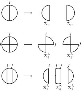
Figure 21: Splitting a knot into other knots.

Combinatorial expressions for the two primitive invariants at order four have been presented in [21]. Their construction is based on the use of the kernels (6.14) and the properties of the perturbative series expansion. As in the case of previous orders, these invariants are expressed in terms of the products (6.12) and the crossing signatures. Their form is more complicated than the ones at lower orders. At order four there are two primitive Vassiliev invariants. We will make the same choice of basis as in [21]. The diagrams associated to them are: $r_{4,2}$ and $r_{4,3}$ in fig. 13. They turn out to be:

$${\hskip 0.0pt}\alpha_{42}(K)=\alpha_{42}(U)+\langle 7\mbox{\leavevmode \hskip 15.0pt}\hbox{\hskip-11.38092pt}+5\mbox{\leavevmode \hskip 15.0pt}\hbox{\hskip-11.38092pt}+4\mbox{\leavevmode \hskip 15.0pt}\hbox{\hskip-11.38092pt}+2\mbox{\leavevmode \hskip 15.0pt}\hbox{\hskip-11.38092pt}+\mbox{\leavevmode \hskip 15.0pt}\hbox{\hskip-11.38092pt}+\mbox{\leavevmode \hskip 15.0pt}\hbox{\hskip-11.38092pt}$$

$$\hbox{\hskip 175.83781pt}+8\mbox{\leavevmode \hskip 15.0pt}\hbox{\hskip-11.38092pt}+2\mbox{\leavevmode \hskip 15.0pt}\hbox{\hskip-11.38092pt}+8\mbox{\leavevmode \hskip 15.0pt}\hbox{\hskip-11.38092pt}+{1\over 6}\mbox{\leavevmode \hskip 15.0pt}\hbox{\hskip-11.38092pt},\bar{G}({\cal K})\rangle$$

$$+\sum_{i,j\in{\cal C}_{a}\atop i>j}\bar{\varepsilon}_{ij}({\cal K})\Bigg{(}\Big{[}\langle\mbox{\leavevmode \hskip 15.0pt}\hbox{\hskip-11.38092pt},G(\alpha({\cal K}))\rangle\Big{]}_{ij}^{a}-2\Big{[}\langle\mbox{\leavevmode \hskip 15.0pt}\hbox{\hskip-11.38092pt},G(\alpha({\cal K}))\rangle\Big{]}_{i}-2\Big{[}\langle\mbox{\leavevmode \hskip 15.0pt}\hbox{\hskip-11.38092pt},G(\alpha({\cal K}))\rangle\Big{]}_{j}\Bigg{)}$$

$$+\sum_{i,j\in{\cal C}_{b}\atop i>j}\bar{\varepsilon}_{ij}({\cal K})\Bigg{(}\Big{[}\langle\mbox{\leavevmode \hskip 15.0pt}\hbox{\hskip-11.38092pt},G(\alpha({\cal K}))\rangle\Big{]}_{ij}^{b}-\Big{[}\langle\mbox{\leavevmode \hskip 15.0pt}\hbox{\hskip-11.38092pt},G(\alpha({\cal K}))\rangle\Big{]}_{i}-\Big{[}\langle\mbox{\leavevmode \hskip 15.0pt}\hbox{\hskip-11.38092pt},G(\alpha({\cal K}))\rangle\Big{]}_{j}\Bigg{)},$$

(6.36)

and,

$${\hskip-2.84544pt}\alpha_{43}(K)=\alpha_{43}(U)+\langle\mbox{\leavevmode \hskip 15.0pt}\hbox{\hskip-11.38092pt}+\mbox{\leavevmode \hskip 15.0pt}\hbox{\hskip-11.38092pt}+\mbox{\leavevmode \hskip 15.0pt}\hbox{\hskip-11.38092pt}+2\mbox{\leavevmode \hskip 15.0pt}\hbox{\hskip-11.38092pt}-{1\over 6}\mbox{\leavevmode \hskip 15.0pt}\hbox{\hskip-11.38092pt},\bar{G}({\cal K})\rangle$$

$$+\sum_{i,j\in{\cal C}_{a}\atop i>j}\bar{\varepsilon}_{ij}({\cal K})\Bigg{(}\Big{[}\langle\mbox{\leavevmode \hskip 15.0pt}\hbox{\hskip-11.38092pt},G(\alpha({\cal K}))\rangle\Big{]}_{ij}^{a}-\Big{[}\langle\mbox{\leavevmode \hskip 15.0pt}\hbox{\hskip-11.38092pt},G(\alpha({\cal K}))\rangle\Big{]}_{i}-\Big{[}\langle\mbox{\leavevmode \hskip 15.0pt}\hbox{\hskip-11.38092pt},G(\alpha({\cal K}))\rangle\Big{]}_{j}\Bigg{)}.$$

(6.37)

In these expressions the explicit dependence on the signatures appears in the quantities $\bar{\varepsilon}_{ij}({\cal K})$ which are:

$$\bar{\varepsilon}_{ij}({\cal K})=\varepsilon_{ij}({\cal K})-\varepsilon_{ij}(\alpha({\cal K}))=\varepsilon_{i}({\cal K})\varepsilon_{j}({\cal K})-\varepsilon_{i}(\alpha({\cal K}))\varepsilon_{j}(\alpha({\cal K})).$$ (6.38)

The sums in which these products are involved are over double splittings of the knot projection ${\cal K}$ at the crossings $i$ and $j$. There are two ways of carrying out these double splittings, depending on the configuration associated to the crossings $i$ and $j$. These are shown in the second and third rows of fig. 21. In the first one the regular projection ${\cal K}$ is split into two while in the second one it is split into three. Splittings of the first type build the set ${\cal C}_{a}$. The ones of the second type build ${\cal C}_{b}$. While only the first one is involved in the invariant $\alpha_{43}$, both appear in $\alpha_{42}$. The new quantities entering the sums are:

$$\Big{[}L({\cal K})\Big{]}_{ij}^{a} = L({\cal K})-L({\cal K}_{ij}^{a_{1}})-L({\cal K}_{ij}^{a_{2}}),$$

$$\Big{[}L({\cal K})\Big{]}_{ij}^{b} = L({\cal K})-L({\cal K}_{ij}^{b_{1}})-L({\cal K}_{ij}^{b_{2}})-L({\cal K}_{ij}^{b_{3}}),$$ (6.39)

where ${\cal K}_{ij}^{a_{1}},{\cal K}_{ij}^{a_{2}},{\cal K}_{ij}^{b_{1}},{\cal K}_{ij}^{b_{2}}$ and ${\cal K}_{ij}^{b_{3}}$ are the knot projections which originate after a double splitting of ${\cal K}$, as denoted in fig. 21. As in previous orders, in the expressions (6.36) and (6.37), the quantities $\alpha_{42}(U)$ and $\alpha_{43}(U)$ correspond to the value of these invariants for the unknot. It has been proved in [21] that the combinatorial expressions for $\alpha_{42}(K)$ and $\alpha_{43}(K)$ in (6.36) and (6.37) are invariant under Reidemeister moves of fig. 2.

Vassiliev invariants constitute vector spaces and their normalization can be chosen in such a way that they are integer-valued. Once their value for the unknot has been subtracted off they can be presented in many basis in which they are integers. We will chose here a particular basis in which the numerical values for the invariants up to order four are rather simple:

$$\nu_{2}(K) = {1\over 4}\tilde{\alpha}_{21}(K),$$

$$\nu_{3}(K) = {1\over 8}\tilde{\alpha}_{31}(K),$$

$$\nu_{4}^{1}(K) = {1\over 8}(\tilde{\alpha}_{42}(K)+\tilde{\alpha}_{43}(K)),$$ (6.40)

$$\nu_{4}^{2}(K) = {1\over 4}(\tilde{\alpha}_{42}(K)-5\tilde{\alpha}_{43}(K)).$$

In these equations the tilde indicates that the value for the unknot has been subtracted, i.e., $\tilde{\alpha}_{ij}(K)=\alpha_{ij}(K)-\alpha_{ij}(U)$. In Tables 1 and 2 we have collected the value of the Vassiliev invariants (6) for all prime knots up to nine crossings. Notice that we could have chosen a basis where all the values for the trefoil knot are 1 just redefining $\nu_{4}^{1}(K)$ into $\nu_{4}^{1}(K)-2\nu_{4}^{2}(K)$. We have no done so because $\nu_{4}^{1}(K)$, as defined in (6), has a simple shape when plotted versus $\nu_{2}(K)$. Actually, the resulting shape has features similar to the shape which results after plotting $\nu_{3}(K)$ versus $\nu_{2}(K)$ (see [23] for more comments in this respect). The similar behavior observed for $|\nu_{3}(K)|$ and $\nu_{4}^{2}(K)$ is expected from their general form for torus knots. As it was shown in [68] and [57], for a torus knot characterized by two coprime integers $p$ and $q$ these invariants are the following polynomials in $p$ and $q$:

$$\nu_{2}(p,q) = {1\over 24}(p^{2}-1)(q^{2}-1),$$

$$\nu_{3}(p,q) = {1\over 144}(p^{2}-1)(q^{2}-1)pq,$$

$$\nu_{4}^{1}(p,q) = {1\over 288}(p^{2}-1)(q^{2}-1)p^{2}q^{2},$$ (6.41)

$$\nu_{4}^{2}(p,q) = {1\over 720}(p^{2}-1)(q^{2}-1)(2p^{2}q^{2}-3p^{2}-3q^{2}-3).$$

The explicit expression of Vassiliev invariants as polynomials in $p$ and $q$ is known up to order six [68]. Of course, up to order four their value agree with the ones computed explicitly from equations (6.36) and (6.37), as it can be checked explicitly from the tables collected below. The only torus knots up to nine crossings are $3_{1}$, $5_{1}$, $7_{1}$, $8_{19}$ and $9_{1}$, whose associated coprime integers are (3,2), (5,2), (7,2), (4,3) and (9,2), respectively.

It would be desirable to write the invariants in such a way that signatures and split sums do not appear. Even better would be to possess expressions where terms involving ascending diagrams are not present. It is not known if this is possible even for the few orders in which combinatorial expressions for the invariants exist. There are indications however that in order to achieve such a goal arrow diagrams as the ones used in [64] have to be introduced. The effect of the introduction of these diagrams is to reduce the amount of embeddings entering the product (6.12) to a selected set. Both, the expressions and the amount of calculation could notably simplify if this is possible. This issue is under investigation.

7 Concluding remarks

In this paper I have presented a brief review of the developments in the context of Chern-Simons gauge theory since the connection between this theory and the theory of knots and links was discovered in 1988. My presentation has started from the basics of both, the physical and mathematical theories, away from the chronological order. I hope to have convinced the reader that the interplay between the physical and mathematical approaches has been very fruitful.

Chern-Simons gauge theory has received the attention of many theoretical physicist and it has been studied from many different points of view. The non-perturbative study led to discover a close connection with the theory of knots and links, which was later further analyzed in detail. Perturbative studies led to new insights in the theory of Vassiliev invariants. These invariants appear in the context of Chern-Simons gauge theory as the coefficients of the perturbative series expansion. Their structure have been analyzed working out the perturbative series expansions for different gauge fixings. Gauge theories are very rich in this respect since they can be studied in different gauges, each providing a particular structure for the coefficients of the perturbative series expansion.

The perturbative analysis of the theory in the covariant Landau gauge led to covariant integral expressions for Vassiliev invariants. These expressions are also known as configuration space integrals. Though important, their from is rather complicated for explicit computations. Simpler expressions for the coefficients appear in non-covariant gauges. In the light-cone gauge one recovers the Kontsevich integral. In the temporal gauge one finds combinatorial expressions. In non-covariant gauges there is an important issue that has not yet been solved. In both, the light-cone and the temporal gauges, one must introduce a factor to find agreement with results in the covariant Landau gauge or with results from a non-perturbative point of view. The origin of this factor, called Kontsevich factor, is not understood. There should exist a field theory argument to justify its presence. The analysis in the temporal gauge indicates that the origin of the factor is not due to a bad choice of the prescription to avoid unphysical poles, a standard problem when dealing with non-covariant gauges. It seems it is related to the presence of a residual gauge invariance. Further work in this respect should be done. Its solution might shed some light on general problems related to non-covariant gauges.

The perturbative analysis in the temporal gauge leads to combinatorial expressions for Vassiliev invariants. We have constructed an approach that avoids integral expressions making use of the factorization theorem. It works very successfully up to order four and, indeed, up to now, this is the only framework which has provided combinatorial expressions for the two primitive Vassiliev invariants at order four. The approach opens a variety of investigations. Certainly, a generalization of the reconstruction procedure from the kernels up to order four should be constructed. This could lead to a general combinatorial formula for Vassiliev invariants. The approach is also well suited to obtain combinatorial expressions for Vassiliev invariants for links, a field which has not been much explored up to now [69]. Another context in which our approach could be also very powerful is in the study of vevs of graphs, quantities that plays an important role in recent developments in the canonical approach to quantum gravity [49]. Vassiliev invariants for graphs constitute a rather unexplored field which could lead to new sets of important invariants.

It is known that polynomial invariants, i.e., vevs of Wilson loops, do not classify knots. On the one hand, polynomial invariants do not distinguish knots that are not invertible (knots which are not equivalent to the ones obtained after reversing their orientation). On the other hand, polynomial invariants do not detect mutant knots which are not equivalent [44]. The question that immediately arises is whether or not Vassiliev invariants, being the coefficients of the power series expansion of Chern-Simons gauge theory, have a chance to classify knots. Fortunately, the answer to this question is affirmative. The polynomial invariants, or vevs of Wilson loops, are associated to a group and a representation (weight system). On the other hand, Vassiliev invariants are the coefficients of the perturbative power series expansion of Chern-Simons gauge theory. Only after making a particular choice of group and representation one makes contact between this series and a polynomial invariant. But one could consider the series as a formal one whose group factors are just the diagrams of the space ${\cal A}$ in (3.5) or (3.6). This space might be bigger than the space of all weight systems and therefore the possibility for Vassiliev invariants to classify knots could still be open. This seems to be the case as shown in [70]. Thus, the set of coefficients of the formal perturbative power series expansion (Vassiliev invariants) is bigger than the set of vevs for any representation and any semi-simple gauge group (polynomial invariants). This is a promising indication that Vassiliev invariants might classify knots. However, simple questions as whether Vassiliev invariants ever detect nonivertibility remains open.

Let me just finish bringing to the attention of the reader the problem of the dimensions of each of the elements of the graded vector space of Vassiliev invariants (3.5) or (3.6). This problem is a very important counting problem which can be addressed from both, a diagrammatic and a group-theoretical point of view. The values of the dimensions are known only up to order 12 [50]. No insight on the problem has been obtained from Chern-Simons gauge theory. Could some field-theoretical method be used to obtain the general solution to this challenging counting problem? This is another important open question which certainly deserves further investigation.

Acknowledgements

I would like to thank my collaborators in Chern-Simons gauge theory all along these ten years, M. Alvarez, L. Alvarez-Gaumé, J. M. Isidro, P. M. Llatas, M. Mariño, E. Pérez and A. V. Ramallo. Their insights have led to understand many of the issues discussed in this paper. I would also like to thank the organizers of the workshop “Trends in Theoretical Physics II”, for inviting me to deliver a lecture and for their warm hospitality. I acknowledge funds provided by the European Commission, which supports the collaboration network ‘CERN-Santiago de Compostela-La Plata’ under contract C11^∗-CT93-0315, for making possible the organization of the workshop. This work is supported in part by DGICYT under grant PB96-0960.

Knot	$\nu_{2}$	$\nu_{3}$	$\nu_{4}^{1}$	$\nu_{4}^{2}$		Knot	$\nu_{2}$	$\nu_{3}$	$\nu_{4}^{1}$	$\nu_{4}^{2}$
$3_{1}$	1	1	3	1		$8_{5}$	$-$1	$-$3	1	$-41$
$4_{1}$	$-$1	0	2	-3		$8_{6}$	$-$2	$-$3	7	-36
$5_{1}$	3	5	25	11		$8_{7}$	2	$-$2	4	22
$5_{2}$	2	3	13	4		$8_{8}$	2	$-$1	5	12
$6_{1}$	$-$2	$-$1	7	$-12$		$8_{9}$	$-$2	0	14	-34
$6_{2}$	$-$1	$-$1	3	$-13$		$8_{10}$	3	$-$3	15	15
$6_{3}$	1	0	0	7		$8_{11}$	$-$1	$-$2	2	-27
$7_{1}$	6	14	98	46		$8_{12}$	$-$3	0	14	$-17$
$7_{2}$	3	6	32	13		$8_{13}$	1	$-$1	$-1$	17
$7_{3}$	5	11	73	25		$8_{14}$	0	0	4	$-16$
$7_{4}$	4	8	50	8		$8_{15}$	4	7	37	18
$7_{5}$	4	8	46	24		$8_{16}$	1	$-$1	$-1$	17
$7_{6}$	1	2	8	-1		$8_{17}$	$-$1	0	6	$-19$
$7_{7}$	$-$1	1	$-$1	3		$8_{18}$	1	0	4	$-9$
$8_{1}$	$-3$	$-3$	13	$-31$		$8_{19}$	5	10	60	35
$8_{2}$	0	$-$1	3	30		$8_{20}$	2	2	8	6
$8_{3}$	$-4$	0	30	$-40$		$8_{21}$	0	$-$1	$-$1	$-14$
$8_{4}$	$-3$	1	21	-39

Table 1: Primitive Vassiliev invariants up to order four for all prime knots up to eight crossings.

Knot	$\nu_{2}$	$\nu_{3}$	$\nu_{4}^{1}$	$\nu_{4}^{2}$		Knot	$\nu_{2}$	$\nu_{3}$	$\nu_{4}^{1}$	$\nu_{4}^{2}$
$9_{1}$	10	30	270	130		$9_{26}$	0	1	$-$5	2
$9_{2}$	4	10	62	32		$9_{27}$	0	1	3	$-6$
$9_{3}$	9	26	228	87		$9_{28}$	1	0	$-$2	3
$9_{4}$	7	19	151	51		$9_{29}$	1	$-$2	2	11
$9_{5}$	6	15	115	20		$9_{30}$	$-$1	$-$1	5	$-9$
$9_{6}$	7	18	134	77		$9_{31}$	2	2	8	6
$9_{7}$	5	12	78	47		$9_{32}$	$-$1	2	$-$2	$-11$
$9_{8}$	0	2	8	-8		$9_{33}$	1	$-$1	3	1
$9_{9}$	8	22	180	80		$9_{34}$	$-$1	0	2	$-3$
$9_{10}$	8	22	188	48		$9_{35}$	7	18	150	13
$9_{11}$	4	$-$9	57	10		$9_{36}$	3	$-$7	39	15
$9_{12}$	1	3	15	1		$9_{37}$	$-$3	1	13	$-7$
$9_{13}$	7	18	142	45		$9_{38}$	6	14	98	46
$9_{14}$	$-$1	2	$-$6	5		$9_{39}$	2	$-$4	24	$-10$
$9_{15}$	2	$-$5	25	4		$9_{40}$	$-$1	$-$1	3	$-13$
$9_{16}$	6	14	94	62		$9_{41}$	0	1	$-$9	18
$9_{17}$	$-$2	0	6	$-2$		$9_{42}$	$-$2	0	10	$-18$
$9_{18}$	6	15	107	52		$9_{43}$	1	2	14	$-13$
$9_{19}$	$-$2	1	3	4		$9_{44}$	0	1	$-1$	10
$9_{20}$	2	4	20	6		$9_{45}$	2	$-$4	20	6
$9_{21}$	3	$-$6	36	$-3$		$9_{46}$	$-$2	$-$3	3	$-20$
$9_{22}$	$-$1	1	1	7		$9_{47}$	$-$1	$-$2	$-$6	5
$9_{23}$	5	11	69	41		$9_{48}$	3	$-$5	29	$-5$
$9_{24}$	1	2	6	$-5$		$9_{49}$	6	14	102	30
$9_{25}$	0	1	11	$-14$

Table 2: Primitive Vassiliev invariants up to order four for all prime knots with nine crossings.

References

- [1]
- [2] E. Witten, Commun. Math. Phys. 121 (1989) 351.
- [3] J. Schonfeld, Nucl. Phys. B185 (1981) 157; R. Jackiw ans S. Templeton, Phys. Rev. D23 (1981) 2291; S. Deser, R. Jackiw ans S. Templeton, Phys. Rev. Lett. 48 975 and Ann. Phys. 140 (1984) 372.
- [4] G.V. Dunne, “Aspects of Chern-Simons Theory”, Les Houches Lectures 1998, hep-th/9902115.
- [5] V. F. R. Jones, Bull. AMS 12 (1985) 103; Ann. of Math. 126 (1987) 335.
- [6] V. A. Vassiliev, “Cohomology of knot spaces”, Theory of singularities and its applications, Advances in Soviet Mathematics, vol. 1, Americam Math. Soc., Providence, RI, 1990, 23-69.
- [7] J.S. Birman, Bull. AMS 28 (1993) 253.
- [8] D. Bar-Natan, Topology 34 (1995) 423.
- [9] J.S. Birman and X.S. Lin, Invent. Math. 111 (1993) 225.
- [10] J.M.F. Labastida and E. Pérez, Nucl. Phys. B527 (1998) 499, hep-th/9712139.
- [11] E. Guadagnini, M. Martellini and M. Mintchev, Phys. Lett. B227 (1989) 111 and B228 (1989) 489; Nucl. Phys. B330 (1990) 575.
- [12] D. Bar-Natan, “Perturbative aspects of Chern-Simons topological quantum field theory”, Ph.D. Thesis, Princeton University, 1991.
- [13] M. Alvarez and J.M.F. Labastida, Nucl. Phys. B395 (1993) 198, hep-th/9110069, and B433 (1995) 555, hep-th/9407076; Erratum, ibid. B441 (1995) 403.
- [14] D. Altschuler and L. Friedel, Commun. Math. Phys. 187 (1997) 261 and 170 (1995) 41.
- [15] R. Bott and C. Taubes, Jour. Math. Phys. 35 (1994) 5247.
- [16] M. Kontsevich, Advances in Soviet Math. 16, Part 2 (1993) 137.
- [17] A.S. Cattaneo, P. Cotta-Ramusino, J. Frohlich and M. Martellini, J. Math. Phys. 36 (1995) 6137.
- [18] J.M.F. Labastida and E. Pérez, J. Math. Phys. 39 (1998) 5183; hep-th/9710176.
- [19] L. Kauffman, “Witten’s Integral and Kontsevich Integral”, preprint.
- [20] S. Poirier, “Rationality Results for the Configuration Space Integral of Knots”, preprint, math.GT/9901028 and “The Limit Configuration Space Integral for Tangles and the Kontsevich Integral”, preprint, math.GT/9902058.
- [21] J.M.F. Labastida and E. Pérez, “Combinatorial Formulae for Vassiliev Invariants from Chern-Simons Gauge Theory”, CERN and Santiago de Compostela preprint, CERN-TH/98-193, US-FT-11/98, to appear in J. Math. Phys.; hep-th/9807155.
- [22] M. Alvarez and J.M.F. Labastida, Commun. Math. Phys. 189 (1997) 641, q-alg/9604010.
- [23] J.M.F. Labastida and E. Pérez, “Vassiliev Invariants in the Context of Chern-Simons Gauge Theory”, Santiago de Compostela preprint, US-FT-18/98; hep-th/9812105.
- [24] M. Goussarov, M. Polyak and O. Viro, “Finite Type Invariants of Classical and Virtual Knots”, preprint, 1998, math.GT/9810073.
- [25] P. Freyd, D. Yetter, J. Hoste, W.B.R. Lickorish, K. Millet and A. Ocneanu, Bull. AMS 12 (1985) 239.
- [26] L.H. Kauffman, Trans. Am. Math. Soc. 318 (1990) 417.
- [27] Y. Akutsu and M. Wadati, J. Phys. Soc. Jap. 56 (1987) 839 and 3039.
- [28] E. Witten, Nucl. Phys. B322 (1989) 629 and B330 (1990) 285.
- [29] C. Kassel, M. Rosso and V. Turaev, “Quantum groups and knot invariants”, Panoramas et syntheses 5, Societe Mathematique de France, 1997.
- [30] C. Kassel and V. Turaev, “Chord diagram invariants of tangles and graphs”, University of Strasbourg preprint, 1995.
- [31] N.Y. Reshetikhin and V. Turaev, Invent. Math. 103 (1991) 547.
- [32] D.S. Freed and R.E. Gompf , Commun. Math. Phys. 141 (1991) 79.
- [33] R. Gambini, private communication.
- [34] R.K. Kaul, “Chern-Simons Theory, Knot Invariants, Vertex Models and Three-Manifold Invariants, hep-th/9804122.
- [35] M. Bos and V.P. Nair, Phys. Lett. B223 (1989) 61 and Int. J. Mod. Phys. A5 (1990) 959.
- [36] J.M.F. Labastida and A.V. Ramallo, Phys. Lett. B227 (1989) 92 and B228 (1989) 214.
- [37] S. Elitzur, G. Moore, A. Schwimmer and N. Seiberg, Nucl. Phys. B326 (1989) 108.
- [38] S. Axelrod, S. Della Pietra and E. Witten, j. Diff. Geom. 33 (1991) 787.
- [39] J. Frohlich and C. King, Commun. Math. Phys. 126 (1989) 167.
- [40] R.K. Kaul and T.R. Govindarajan, Nucl. Phys. B380 (1992) 293 and B393 (1993) 392; P. Ramadevi, T.R. Govindarajan and R.K. Kaul, Nucl. Phys. B402 (1993) 548; R.K. Kaul, Commun. Math. Phys. 162 (1994) 289.
- [41] S. Martin, Nucl. Phys. B338 (1990) 244.
- [42] J.M.F. Labastida, P.M. Llatas and A.V. Ramallo, Nucl. Phys. B348 (1991) 651; J.M.F. Labastida and M. Mariño, Int. J. Mod. Phys. A10 (1995) 1045; J.M.F. Labastida and E. Pérez, J. Math. Phys. 37 (1996) 2013.
- [43] P. Ramadevi, T.R. Govindarajan and R.K. Kaul, Mod. Phys. Lett. A9 (1994) 3205.
- [44] P. Ramadevi, T.R. Govindarajan and R.K. Kaul, Mod. Phys. Lett. A10 (1995) 1635.
- [45] J. M. Isidro, J. M. F. Labastida and A. V. Ramallo, Phys. Lett. B282 (1992) 63; Nucl. Phys. B398 (1993) 187; I. P. Ennes, P. Ramadevi, A. V. Ramallo and J. M. Sanchez de Santos, Int. J. Mod. Phys. A13 (1998) 2931.
- [46] R.K. Kaul, Nucl. Phys. B417 (1994) 267; P. Ramadevi, T.R. Govindarajan and R.K. Kaul, Nucl. Phys. B422 (1994) 291.
- [47] Carlo Rovelli and Lee Smolin, Phys. Rev. Lett. 68 (1992) 431; Nucl. Phys. B385 (1992) 587.
- [48] B. Bruegmann, R. Gambini and J. Pullin, Phys. Rev. Lett. 61 (1988) 1155; Nucl. Phys. B331 (1990) 80.
- [49] R. Gambini, J. Griego and J. Pullin, Phys. Lett. B425 (1998) 41 and Nucl. Phys. B534 (1998) 675.
- [50] J. A. Kneissler, “The number of primitive Vassiliev invariants up to degree 12”, Math. Inst. Bonn, 1997, q-alg/9706022.
- [51] D. Thurston, “Integral expressions for the Vassiliev knot Invariants”, Harvard University senior thesis, April 1995; math/9901110.
- [52] S. Axelrod and I.M. Singer, “Chern-Simons Perturbation Theory”, 1991, hep-th/9110056 and J. Diff. Geom. 39 (1994) 173.
- [53] W. Chen, G.W. Semenoff, and Y.-S. Wu, Mod. Phys. Lett. A5 (1990) 1833.
- [54] L. Alvarez-Gaumé, J.M.F. Labastida and A. V. Ramallo, Nucl. Phys. B334 (1990) 103; G. P. Korchemsky, Mod. Phys. Lett. A6 (1991) 727.
- [55] C.P. Martin, Phys. Lett. B241 (1990) 513; G. Giavarini, C.P. Martin, F. Ruiz Ruiz, Nucl. Phys. B381 (1992) 222, Phys. Lett. B314 (1993) 328, Phys. Rev. D47 (1993) 5536 and Phys. Lett. B332 (1994) 345.
- [56] M. Asorey and F. Falceto, Phys. Lett. B241 (1990) 31; M. Asorey, F. Falceto, J.L. Lopez and G. Luzon, Phys. Rev. D49 (1994) 5377 and Nucl. Phys. B429 (1994) 344.
- [57] S. Willerton, “On Universal Vassiliev Invariants, Cabling, and Torus Knots”, University of Melbourne preprint (1998).
- [58] S.-W. Yang, “Feynman integral, knot invariant and degree theory of maps”, National Taiwan University preprint, September 1997; q-alg/9709029.
- [59] A.C. Hirshfeld and U. Sassenberg, Journal of Knot Theory and its Ramifications 5 (1996) 489 and 5 (1996) 805.
- [60] G. Leibbrandt and C.P. Martin, Nucl. Phys. B377 (1992) 593 and B416 (1994) 351.
- [61] A. Brandhuber, S. Emery, M. Langer, O. Piguet, M. Schweda and S.P. Sorella, Helv. Phys. Acta 66 (1993) 551.
- [62] G. Leibbrandt, Rev. Mod. Phys. 59 (1987) 1067.
- [63] T.Q.T. Le and J. Murakami, “The universal Vassiliev-Kontsevich invariant for framed oriented links”, Max-Plank Institut fur Mathematik preprint, 1994.
- [64] M. Goussarov, M. Polyak and O. Viro, Int. Math. Res. Notices 11 (1994) 445.
- [65] J.F.W.H. van de Wetering, Nucl. Phys. B379 (1992) 172.
- [66] L. H. Kauffman, “Virtual Knot Theory”, preprint, 1998.
- [67] P. Lannes, L’Enseignement Math. 39 (1993) 295.
- [68] M. Alvarez and J.M.F. Labastida, Journal of Knot Theory and its Ramifications 5 (1996) 779; q-alg/9506009.
- [69] M. Alvarez, J.M.F. Labastida and E. Pérez, Nucl. Phys. B488 (1997) 677.
- [70] Pierre Vogel, Algebraic structures on modules of diagrams, Université Paris VII preprint, July 1995.