MIT–CTP–2857 UCLA/99/TEP/16 hep-th/9905049

AdS/CFT 4–point functions:

How to succeed at $z$–integrals without really trying

Eric D’Hoker^a, Daniel Z. Freedman^b,c, and Leonardo Rastelli^b,

^a Department of Physics

University of California, Los Angeles, CA 90095

and Institute for Theoretical Physics

University of California, Santa Barbara, CA 93106

^b Center for Theoretical Physics

Massachusetts Institute of Technology

Cambridge, MA 02139

^c Department of Mathematics

Massachusetts Institute of Technology

Cambridge, MA 02139

A new method is discussed which vastly simplifies one of the two integrals over $AdS_{d+1}$ required to compute exchange graphs for 4–point functions of scalars in the AdS/CFT correspondence. The explicit form of the bulk–to–bulk propagator is not required. Previous results for scalar, gauge boson and graviton exchange are reproduced, and new results are given for massive vectors. It is found that precisely for the cases that occur in the $AdS_{5}\times S_{5}$ compactification of Type IIB supergravity, the exchange diagrams reduce to a finite sum of graphs with quartic scalar vertices. The analogous integrals in $n$–point scalar diagrams for $n>4$ are also evaluated.

1 Introduction

During the past year several groups have calculated 4–point correlation functions in AdS supergravity as part of the study of the AdS/CFT correspondence [1, 2, 3]. In particular the position space correlators for quartic scalar interactions [4, 5] , gauge boson exchange [6], scalar field exchange [7, 8], and graviton exchange [9] have been obtained. There is additional work on a momentum space approach [10].

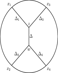
Exchange diagrams, see Figure 1, contain a bulk–to–bulk propagator, and two integrations over $AdS_{d+1}$ are required to compute the amplitude. In past work the first integral, called the $z$–integral, was calculated by a cumbersome expansion and resummation procedure which typically gave a simple function of the other bulk coordinate $w_{\mu}$ as result. This suggests that a more direct method should be possible, and it is the main purpose of the present paper to present one. Specifically we show that $z$–integrals satisfy a simple differential equation which can be solved recursively. The specific form of the bulk–to–bulk propagator is not required. All previous cases can be handled quite easily by the new method, and we are also able to obtain new results for massive vector exchange amplitudes as well as for higher point correlators. The new method does not simplify the remaining integral over the $w_{\mu}$ coordinate, and we refer to past work [6, 8, 9] in which useful integral representations and asymptotic formulas for these $w$–integrals have been derived.

Our main focus of interest is the $AdS_{5}\times S_{5}$ compactification of IIB supergravity [11], but clearly the method we propose, and most of our formulas, have a general validity. We do not discuss certain subtleties that occur in $d=2$ for massless vector and graviton equations, which would require a more careful investigation of asymptotics and are left to future work (hopefully by someone else).

In all the exchange graphs that we study, it is found that precisely for the trilinear couplings that occur in the $AdS_{5}\times S_{5}$ supergravity, the exchange diagram reduces to a finite sum of scalar quartic graphs. Generic couplings give instead an infinite sum. We lack a fundamental explanation of this fact, although we suspect some simple mathematical reason related to harmonic analysis on $S_{5}$ and representation theory of the conformal group $SO(5,1)$. It would be interesting to check whether the same holds for other supergravity compactifications of interest in the AdS/CFT correspondence (for example [12]).

The basic idea is presented in Section 2 for scalar exchange. Massless and massive vector exchange is discussed in Section 3, and graviton exchange in Section 4. In Section 5 we discuss an application to $n$–point correlators for $n\geq 5$.

                                                                                                                                                          

Figure 1: A general t–channel exchange diagram.

2 Scalar exchange

As in most past work, we calculate on the Euclidean continuation of $AdS_{d+1}$, which is modelled as the upper half space $z_{\mu}\in{\bf R}^{d+1}$, with $z_{0}>0$, and metric $g_{\mu\nu}$ of constant negative curvature $R=-d(d+1)$, given by

$$ds^{2}=\sum_{\mu,\nu=0}^{d}g_{\mu\nu}dz_{\mu}dz_{\nu}={1\over z_{0}^{2}}(dz^{2}_{0}+\sum^{d}_{i=1}\,dz^{2}_{i})\,.$$ (2.1)

The Christoffel symbols are

$$\Gamma^{\kappa}_{\mu\nu}={1\over{z_{0}}}\bigl{(}\delta_{0}^{\kappa}\delta_{\mu\nu}-\delta_{\mu 0}\delta^{\kappa}_{\nu}-\delta_{\nu 0}\delta^{\kappa}_{\mu}\bigr{)}\,.$$ (2.2)

It is well-known that AdS–invariant functions, such as scalar propagators, are simply expressed [13] as functions of the chordal distance $u$, defined by

$$u={(z-w)^{2}\over 2z_{0}w_{0}}\qquad\qquad(z-w)^{2}=\delta_{\mu\nu}(z-w)_{\mu}(z-w)_{\nu}$$ (2.3)

A scalar field of mass $m^{2}$ is characterized by two possible scale dimensions, namely the roots

$$\Delta_{\pm}=\frac{d}{2}\pm\frac{1}{2}\sqrt{d^{2}+4m^{2}}$$ (2.4)

of the quadratic relation $m^{2}=\Delta(\Delta-d)$. The mass must satisfy the bound [14] $m^{2}\geq-d^{2}/4$. For $m^{2}\geq-d^{2}/4+1$, one must choose the largest root $\Delta=\Delta_{+}$. In the range $-d^{2}/4<m^{2}<-d^{2}/4+1$, the bulk field may be quantized with either dimension $\Delta_{\pm}$, and it is known that supersymmetry can require both choices to occur in the same theory. Only the largest root appears in most applications of the AdS/CFT correspondence, but we will need to discuss the other possibility briefly. Unless explicitly indicated $\Delta$ will mean $\Delta_{+}$.

The scalar bulk–to–bulk propagator for dimension $\Delta=\Delta_{\pm}$ was obtained in [13],

$$G_{\Delta}(u) = \tilde{C}_{\Delta}(2u^{-1})^{\Delta}F\bigl{(}\Delta,\Delta-{d\over 2}+{1\over 2};2\Delta-d+1;-2u^{-1}\bigr{)}$$ (2.5)

$$\tilde{C}_{\Delta} = {\Gamma(\Delta)\Gamma(\Delta-{d\over 2}+{1\over 2})\over(4\pi)^{(d+1)/2}\Gamma(2\Delta-d+1)}$$ (2.6)

where $F$ is the standard hypergeometric function ${}_{2}F_{1}$. The propagator satisfies the differential equation

$$(-\Box+m^{2})G_{\Delta}(u)=\delta(z,w)$$ (2.7)

The scalar bulk–to–boundary propagator for dimension $\Delta$ is given by [3]

$$K_{\Delta}(z,\vec{x})=\left({z_{0}\over z^{2}_{0}+\left(\vec{z}-\vec{x}\right)^{2}}\right)^{\Delta}\,,$$ (2.8)

where $\vec{x}$ indicates a point on the $d$–dimensional boundary of $AdS_{d+1}$. In this paper we systematically omit the normalization factors for bulk–to–boundary propagators [15],

$$C_{\Delta}={\Gamma(\Delta)\over\pi^{d/2}\Gamma(\Delta-d/2)}\,.$$ (2.9)

The integrals we have to evaluate take the form

$$S(\vec{x}_{1},\vec{x}_{2},\vec{x}_{3},\vec{x}_{4})=\int{d^{d+1}w\over w^{d+1}_{0}}\,A(w,\vec{x_{1}},\vec{x_{3}})\,K_{\Delta_{2}}(w,\vec{x}_{2})K_{\Delta_{4}}(w,\vec{x}_{4})\,,$$ (2.10)

where

$$A(w,\vec{x_{1}},\vec{x_{3}})=\int{d^{d+1}z\over z^{d+1}_{0}}G_{\Delta}(u)K_{\Delta_{1}}(z,\vec{x}_{1})K_{\Delta_{3}}(z,\vec{x}_{3})\,.$$ (2.11)

All scaling dimensions will be always understood to be $\geq\frac{d}{2}$. More general integrals with derivative couplings can be reduced to this case (see for example (A.5) in [9]). In this paper we develop a new method to calculate the $z$–integrals (2.11). The remaining $w$–integral (2.10) can then be handled by the asymptotic expansion techniques developed in [6, 8, 9].

As in past work, the integral (2.11) is considerably simplified by performing the translation $\vec{x}_{1}\to 0$, $\vec{x}_{3}\to\vec{x}_{31}\equiv\vec{x}_{3}-\vec{x}_{1}$ and the conformal inversion

$$\vec{x}_{13}=\frac{\vec{x}^{\prime}_{13}}{|\vec{x}^{\prime}_{13}|^{2}}\qquad z_{\mu}=\frac{z^{\prime}_{\mu}}{(z^{\prime})^{2}}\qquad w_{\mu}=\frac{w^{\prime}_{\mu}}{(w^{\prime})^{2}}\,.$$ (2.12)

The integral takes the form

$$A(w,\vec{x}_{1},\vec{x}_{3})=|\vec{x}_{13}|^{-2\Delta_{3}}\,I(w^{\prime}-\vec{x}^{\prime}_{13})$$ (2.13)

where

$$I(w)=\int{d^{d+1}z\over z^{d+1}_{0}}\,G_{\Delta}(u)\,(z_{0})^{\Delta_{1}}\left(\frac{z_{0}}{z^{2}}\right)^{\Delta_{3}}\,.$$ (2.14)

Convergence of the integral requires $\Delta>|\Delta_{1}-\Delta_{3}|$, and we assume that this condition, and the previous conditions $\Delta,\Delta_{i}\geq\frac{d}{2}$ hold in the following. Integrals of this form with scalar, vector, and symmetric tensor bulk–to–bulk propagators are the main focus of this paper.

Let us first discuss briefly the old method for evaluating the integral and then the new one. In the old method a quadratic transformation of the hypergeometric function, namely

$$G_{\Delta}(u)=2^{\Delta}\tilde{C}_{\Delta}\xi^{\Delta}F\big{(}\frac{\Delta}{2},\frac{\Delta}{2}+{1\over 2};\Delta-{d\over 2}+1;\xi^{2}\big{)}\,$$ (2.15)

with variable

$$\xi\equiv{1\over 1+u}={2z_{0}w_{0}\over z^{2}_{0}+w^{2}_{0}+(\vec{z}-\vec{w})^{2}}\,$$ (2.16)

was used. The propagator was then expressed as a power series in $\xi$ and the $z$–integral was done term by term using Feynman parameters. The resulting series, usually a geometric series, was then resummed. For favorable relations among the dimensions $\Delta$, $\Delta_{1}$, $\Delta_{3}$, and $d$, relations which cover all the cases in the application of the AdS/CFT correspondence to the $d=4$, ${\cal N}=4$ superymmetric Yang–Mills theory, the Feynman parameter integral could also be done and the result for $I(w)$ was a simple polynomial in the variable $w_{0}^{2}/w^{2}$.

The new method is ultra–simple for scalar exchange. We first note that invariance of $I(w)$ under the scale transformation $w_{\mu}\to\lambda w_{\mu}$ and under the $d$–dimensional Poincare subgroup of $SO(d+1,1)$ implies that $I(w)$ can be represented as

$$I(w)=(w_{0})^{\Delta_{13}}f(t)$$ (2.17)

where

$$t=\frac{w_{0}^{2}}{w^{2}}=\frac{w_{0}^{2}}{w_{0}^{2}+|\vec{w}|^{2}}$$ (2.18)

and $\Delta_{13}\equiv\Delta_{1}-\Delta_{3}$. Next we apply the wave operator $(-\Box+m^{2})$ to $I(w)$ and use (2.7) to obtain

$$(-\Box+m^{2})[(w_{0})^{\Delta_{13}}f(t)]=(w_{0})^{\Delta_{13}}t^{\Delta_{3}}\,.$$ (2.19)

The next step is to work out the action of the Laplacian on the left side, which leads to the inhomogeneous second order differential equation for $f(t)$

$$4t^{2}(t-1)f^{\prime\prime}+4t[(\Delta_{13}+1)t-\Delta_{13}+\frac{d}{2}-1]f^{\prime}+[\Delta_{13}(d-\Delta_{13})+m^{2}]f=t^{\Delta_{3}}$$ (2.20)

The particular solution that corresponds to the actual value of the integral (2.14) is selected by the following asymptotic conditions on $f(t)$:

1. Since $I(w)$ is perfectly regular at $\vec{w}=0$, $f(t)$ must be smooth as $t\to 1$.

2. In the limit $w_{0}\to 0$ we have from (2.5) and (2.3) that $I(w)\sim w_{0}^{\Delta}$, which implies $f(t)\sim t^{\frac{\Delta-\Delta_{13}}{2}}$ as $t\to 0$. (Recall that we are considering the case $\Delta=\Delta_{+}$).

The differential operator in (2.20) is closely related to the hypergeometric operator, and we will discuss this shortly, but for the cases of interest we can find a particular solution of the equation more quickly if we convert it to a recursion relation. To do this we assume the series representation

$$f(t)=\sum_{k}a_{k}t^{k}\,.$$ (2.21)

Upon substitution in (2.20) we find a recursion relation for the coefficients which works downwards in $k$. We can consistently set $a_{k}=0$ for $k\geq\Delta_{3}$. We then get

$$a_{k} = 0\qquad{\rm for}\;k\geq\Delta_{3}$$ (2.22)

$$a_{\Delta_{3}-1} = \frac{1}{4(\Delta_{1}-1)(\Delta_{3}-1)}$$ (2.23)

$$a_{k-1} = \frac{(k-\frac{\Delta}{2}+\frac{\Delta_{13}}{2})(k-\frac{d}{2}+\frac{\Delta}{2}+\frac{\Delta_{13}}{2})}{(k-1)(k-1+\Delta_{13})}\;a_{k}$$ (2.24)

Note that $k$ need not take integer values, rather $k=\Delta_{3}+l$ with $l$ integer but $\Delta_{3}$ arbitrary. We now observe that the series terminates at the positive value $k_{{\rm min}}=(\Delta-\Delta_{13})/2\leq k_{{\rm max}}=\Delta_{3}-1$ provided that $\Delta_{1}+\Delta_{3}-\Delta$ is a positive even integer. If (and only if) this condition is satisfied, (2.21–2.24) give a well–defined particular solution of (2.20) with the required asymptotic properties. We will shortly prove its uniqueness.

It is pleasant to observe that the condition for terminating series is satisfied for all the cases that occur in type IIB $AdS_{5}\times S_{5}$ supergravity [11] due to restrictions on trilinear couplings from $SU(4)$ symmetry [16, 8]. In this paper we will only consider the terminating case.

We can easily prove uniqueness of the solution (2.21–2.24) by showing that any combination of the two homogeneous solutions of (2.20) fails to satisfy the asymptotic requirements on $f(t)$. By making the change of variable $x=1/t$, we can write the homogeneous equation as

$$x(1-x)f^{\prime\prime}(x)+[1-\Delta_{13}-(1-\Delta_{13}+\frac{d}{2})x]f^{\prime}(x)-\frac{1}{4}(\Delta_{13}-\Delta)(\Delta_{13}+\Delta-d)f(x)=0$$ (2.25)

which is the hypergeometric equation of parameters $a=\frac{\Delta-\Delta_{13}}{2}$, $b=\frac{d-\Delta-\Delta_{13}}{2}$, $c=1-\Delta_{13}$. Two independent homogeneous solutions of (2.20) are then given by [17]

$$f_{1}(t) = t^{\frac{\Delta-\Delta_{13}}{2}}F(\frac{\Delta-\Delta_{13}}{2},\frac{\Delta+\Delta_{13}}{2};\Delta-\frac{d}{2}+1;t)$$ (2.26)

$$f_{2}(t) = F(\frac{\Delta-\Delta_{13}}{2},\frac{d-\Delta-\Delta_{13}}{2};\frac{d}{2};1-\frac{1}{t})$$ (2.27)

It is easy to see that $f_{1}$ is singular for $t\to 1$, while $f_{2}$ is regular in the same limit. We must then reject $f_{1}$ based on the first asymptotic condition stated above. For $t\to 0$, $f_{2}(t)\sim t^{\frac{d-\Delta-\Delta_{13}}{2}}$, which violates the second asymptotic condition. $f_{2}$ scales at small $t$ with the rate corresponding to the “irregular” choice of boundary condition for the bulk scalar, i.e. $\Delta=\Delta_{-}$. The value of the integral (2.14) for $\Delta=\Delta_{-}$ could be obtained in the terminating case by adding to the particular solution (2.21–2.24) a multiple of $f_{2}$.

We now make contact with the results of [8]. The restriction of $\Delta_{1}+\Delta_{3}-\Delta$ to positive even integers agrees with the condition stated after (3.22) of [8] for termination of the (transformed) hypergeometric series in (3.10) or (3.11). The integral in (3.11) then yields a polynomial expression wich precisely agrees with (2.21–2.24). Note that the integral $I(w)$ was called $R(w)$ in [8].

We can finally assemble the result for the initial amplitude (2.10). From (2.13), (2.17–2.18), (2.21), inverting back to the original coordinates $\vec{x}_{i}$ (see (2.12)), we have

$$S(\vec{x}_{1},\vec{x}_{2},\vec{x}_{3},\vec{x}_{4})=$$ (2.28)

$$\sum_{k_{\rm min}}^{k_{\rm max}}a_{k}\,|\vec{x}_{13}|^{-2\Delta_{3}+2k}\int{d^{d+1}w\over w^{d+1}_{0}}\,K_{\Delta_{1}-\Delta_{3}+k}(w,\vec{x}_{1})\,K_{k}(w,\vec{x}_{3})\,K_{\Delta_{2}}(w,\vec{x}_{2})\,K_{\Delta_{4}}(w,\vec{x}_{4})\,,$$

i.e. the exchange amplitude reduces to a finite sum of scalar quartic graphs. The analytic properties of these quartic graphs have been extensively studied [4, 5, 6, 8, 9]. In particular asymptotic expansions in terms of conformally invariant variables are available. We refer the reader to Section 6 and to Appendix A of [9] for a self–contained derivation of these expansions and of many other useful identities.

3 Vector exchange

The basic procedure for vector and tensor exchange integrals is the same as in the scalar case. We use the wave equation satisfied by the bulk–to–bulk propagator to turn the integral into an inhomogeneous second order differential equation for scalar functions of $t=(w_{0})^{2}/w^{2}$ and then obtain the particular solution with required asymptotics by a recursion relation. The choice of a suitable ansatz which expresses the vector or tensor valued integral in terms of scalar functions and the action of the wave operator on that ansatz are more complicated than in the scalar case.

For vector exchange we study the integrals

$$V(\vec{x}_{1},\vec{x}_{2},\vec{x}_{3},\vec{x}_{4})=\int\frac{d^{d+1}w}{w_{0}^{d+1}}\,A_{\mu}(w,\vec{x}_{1},\vec{x}_{3})\;g^{\mu\nu}(w)\;K_{\Delta_{2}}(w,\vec{x}_{2})\frac{\stackrel{{\scriptstyle\leftrightarrow}}{{\partial}}}{\partial w_{\mu}}K_{\Delta_{2}}(w,\vec{x}_{4})$$ (3.1)

where

$$A_{\mu}(w,\vec{x}_{1},\vec{x}_{3})=\int\frac{d^{d+1}z}{z_{0}^{d+1}}\,G_{\mu\nu^{\prime}}(w,z)\,g^{\nu^{\prime}\rho^{\prime}}(z)\,K_{\Delta_{1}}(z,\vec{x}_{1})\frac{\stackrel{{\scriptstyle\leftrightarrow}}{{\partial}}}{\partial z_{\rho^{\prime}}}K_{\Delta_{1}}(z,\vec{x}_{3})$$ (3.2)

Note that we use unprimed indices for the $w$ coordinate and primed indices for $z$. The only information we need about the bulk–to–bulk propagator is the defining wave equation, namely

$$-\frac{1}{\sqrt{g}}\partial_{\mu}(\sqrt{g}g^{\mu\lambda}\partial_{[\lambda}G_{\rho]\nu^{\prime}}(w,z))+m^{2}G_{\rho\nu^{\prime}}(w,z)=g_{\rho\nu^{\prime}}\delta(w,z)+\partial_{\mu}\partial_{\nu^{\prime}}\Lambda(u)$$ (3.3)

where the first term is the Maxwell operator and the second is the mass term. The pure gauge term appears on the right side only for $m^{2}=0$ because the operator is then non–invertible. For $m^{2}\neq 0$, this is the appropriate wave equation for the massive vector fields of type IIB supergravity on $AdS_{5}\times S_{5}$ [11]. We have also assumed that vectors couple to the conserved current formed from the two bulk–to–boundary propagators in (3.2). This is certainly the case for massless gauge bosons, and we restrict attention to conserved current sources for massive KK vectors also. The method can be extended to include more general sources.

The propagator transforms as a bitensor under inversion, so the integral transforms to the inverted frame as [15]

$$A_{\mu}(w,\vec{x}_{1},\vec{x}_{3})=|\vec{x}_{13}|^{-2\Delta_{1}}\frac{1}{w^{2}}J_{\mu\nu}(w)I_{\nu}(w^{\prime}-\vec{x}^{\prime}_{13})$$ (3.4)

where $J_{\mu\nu}(w)=\delta_{\mu\nu}-2\,w_{\mu}w_{\nu}/w^{2}$ and

$$I_{\mu}(w)=\int\frac{d^{d+1}z}{z_{0}^{d+1}}\,G_{\mu}^{\;\;\nu^{\prime}}(w,z)\,\,z_{0}^{\Delta_{1}}\frac{\stackrel{{\scriptstyle\leftrightarrow}}{{\partial}}}{\partial z_{\nu^{\prime}}}\left(\frac{z_{0}}{z^{2}}\right)^{\Delta_{1}}\,.$$ (3.5)

We now need a suitable ansatz for the vector function $I_{\mu}(w)$. Scale symmetry and $d$–dimensional Poincaré symmetry suggest the form

$$I_{\mu}(w)={w_{\mu}\over w^{2}}f(t)+{\delta_{\mu 0}\over w_{0}}h(t)$$ (3.6)

However, the second term can be dropped because of the following argument. The first step is the observation that $D^{\mu}I_{\mu}(w)=0$. This follows because the divergence $D^{\mu}G_{\mu\nu^{\prime}}(w,z)$ is a rank 1 bitensor in a maximally symmetric space, and must then be proportional to the only independent rank 1 bitensor [19], namely $\partial_{\nu^{\prime}}u$, times a scalar function of $u$. $D^{\mu}G_{\mu\nu^{\prime}}(w,z)$ can then be expressed as a $z$–derivative of a scalar function:

$$D^{\mu}G_{\mu\nu^{\prime}}(w,z)=\partial_{\nu^{\prime}}u\,g(u)=\partial_{\nu^{\prime}}\left(\int g(u)\right)\,.$$ (3.7)

This gradient term can then be partially integrated in the $z$–integral for $D^{\mu}I_{\mu}(w)=0$ and vanishes by current conservation. The divergence can now be applied to the ansatz (3.6), which gives

$$0=D^{\mu}I_{\mu}(w)=D^{\mu}\left({w_{\mu}\over w^{2}}f(t)\right)+D^{\mu}\left({\delta_{\mu 0}\over w_{0}}h(t)\right)$$ (3.8)

The first term vanishes identically, while the second term leads to a separable first order homogeneous equation for $h(t)$. The non–trivial solution is singular as $t\rightarrow 1$ and must be rejected, since we see by inspection of (3.2) that $I_{\mu}(w)$ is regular there. Thus we have proven that $h(t)=0$ and we can use the representation

$$I_{\mu}(w)={w_{\mu}\over w^{2}}\,f(t).$$ (3.9)

We now apply the wave operator to $I_{\mu}(w)$, and use (3.3) under the integral sign (the gauge term vanishes when integrated by parts). The result is the equation

$$-\frac{1}{\sqrt{g}}\partial_{\mu}\left(\sqrt{g}g^{\mu\lambda}\partial_{[\lambda}\left(\frac{w_{\rho]}}{w^{2}}f(t)\right)\right)+m^{2}\,\frac{w_{\rho}}{w^{2}}\,f(t)=-2\Delta_{1}{w_{\rho}\over w^{2}}\,t^{\Delta_{1}}\,.$$ (3.10)

It is now straightforward, although complicated, to calculate the result of the action of the Maxwell operator on the left side, and this leads to the differential equation

$$4t^{2}(t-1)f^{\prime\prime}+4t(2t+{{d-4}\over 2})f^{\prime}+m^{2}f=-2\Delta_{1}\,t^{\Delta_{1}}\,.$$ (3.11)

This inhomogeneous differential equation is clearly of the same type as (2.20) for scalar exchange. We thus proceed in the same way by looking for a particular solution of the form

$$f(t)=\sum_{k}a_{k}t^{k}\,.$$ (3.12)

with $k\in\{k_{{\rm min}},k_{{\rm min}}+1,\dots,k_{{\rm max}}\}$. We find:

$$a_{k} = 0\qquad{\rm for}\;k\geq\Delta_{1}$$ (3.13)

$$a_{\Delta_{1}-1} = \frac{1}{2(\Delta_{1}-1)}$$ (3.14)

$$a_{k-1} = \frac{2k(2k+2-d)-m^{2}}{4(k-1)k}\;a_{k}\,.$$ (3.15)

The series terminates at $0<k_{{\rm min}}=\frac{d-2}{4}+\frac{1}{4}\sqrt{(d-2)^{2}+4m^{2}}\leq k_{{\rm max}}=\Delta_{1}-1$ provided that $k_{{\rm max}}-k_{{\rm min}}$ is integer and $\geq 0$. It is easy to check, in analogy with the scalar case, that if this condition is obeyed, (3.12–3.15) define the unique particular solution of (3.11) with the correct asymptotic properties to correspond to the actual value of the integral (3.2). For $m^{2}=0$ and $d=2$, the coefficient $a_{k_{\rm min}}=a_{0}$ is infinite, a signal that this case requires special attention.

We now consider the application of these results to the $AdS_{5}\times S_{5}$ compactification of IIB supergravity. From Table III in [11], we see that the allowed values of the mass for KK vectors are $m^{2}=(l-1)(l+1)$, with $l$ integer $\geq 1$. The termination condition then requires $\Delta_{1}-1-(1/2+l/2)$ be a non–negative integer, which restricts $l$ to be odd and $<2\Delta_{1}-1$. It can be shown that $SU(4)$ selection rules [16] enforce $l$ odd, $l\leq 2\Delta_{1}-1$. In fact, the value of $l$ correlates to the quadrality of the $SU(4)$ representation of the vector field, the quadrality is 0 or 2 for $l$ odd or even. Since scalar fields come in representations with quadrality 2 or 0, and we are assuming two equal scalar fields $\Delta_{1}=\Delta_{3}$, imposing that the sum of the quadralities in the trilinear coupling is 0 mod 4 forces $l$ to be odd. The inequality $l\leq 2\Delta-1$ is the standard “Clebsch–Gordon” triangle inequality. We thus observe the nice phenomenon that precisely for the cases allowed in the supergravity we get terminating series for the vector exchange $z$–integrals.

We now wish to compare with the results of [6], where the massless vector exchange was computed. For $m=0$, the termination condition requires $\Delta_{1}-d/2$ be a non–negative integer, which is in particular satisfied for $d$ even and $\Delta_{1}$ integer satisfying the unitarity bound. This is the condition stated in [6] after (3.21) for the $z$–integral (3.20) to reduce to a finite sum of elementary terms. Comparison with the results of the present paper shows perfect agreement.

4 Graviton exchange

The tensor exchange integral is more complicated than previous cases, although the new method is still considerably simpler than that of previous work [9]. We start with the integral

$$G(\vec{x}_{1},\vec{x}_{2},\vec{x}_{3},\vec{x}_{4})=\int\frac{d^{d+1}w}{w_{0}^{d+1}}\,A^{\mu\nu}(w,\vec{x}_{1},\vec{x}_{3})\;T_{\mu\nu}(w,\vec{x}_{2},\vec{x}_{4})$$ (4.1)

where

$$A_{\mu\nu}(w,\vec{x}_{1},\vec{x}_{3})=\int\frac{d^{d+1}z}{z_{0}^{d+1}}\,G_{\mu\nu\mu^{\prime}\nu^{\prime}}(w,z)T^{\mu^{\prime}\nu^{\prime}}(z,\vec{x}_{1},\vec{x}_{3})\,.$$ (4.2)

The stress tensor governing the couplings of the bulk graviton to scalar fields of equal dimensions $\Delta_{1}=\Delta_{3}=\frac{d}{2}+\frac{1}{2}\sqrt{{d^{2}}+4m_{1}^{2}}$ is given by

$$T^{\mu^{\prime}\nu^{\prime}}(z,\vec{x}_{1},\vec{x}_{3}) = ~{}D^{\mu^{\prime}}K_{\Delta_{1}}(z,\vec{x}_{1})D^{\nu^{\prime}}K_{\Delta_{1}}(z,\vec{x}_{3})$$

$$-\frac{1}{2}\,g^{\mu^{\prime}\nu^{\prime}}\bigl{[}D_{\rho^{\prime}}K_{\Delta_{1}}(z,\vec{x}_{1})D^{\rho^{\prime}}K_{\Delta_{1}}(z,\vec{x}_{3})+m_{1}^{2}K_{\Delta_{1}}(z,\vec{x}_{1})K_{\Delta_{1}}(z,\vec{x}_{3})\bigr{]}\,.$$

The graviton propagator $G_{\mu\nu\mu^{\prime}\nu^{\prime}}(w,z)$ was discussed extensively in [18], but the main property needed here is the (Ricci form) of its wave equation, namely

$$W_{\mu\nu}^{\;\;\;\lambda\rho}G_{\lambda\rho\mu^{\prime}\nu^{\prime}} \equiv -D^{\sigma}D_{\sigma}G_{\mu\nu\mu^{\prime}\nu^{\prime}}-D_{\mu}D_{\nu}G_{\sigma}{}^{\sigma}{}_{\mu^{\prime}\nu^{\prime}}+D_{\mu}D^{\sigma}G_{\sigma\nu\mu^{\prime}\nu^{\prime}}$$

$$+D_{\nu}D^{\sigma}G_{\mu\sigma\mu^{\prime}\nu^{\prime}}-2(G_{\mu\nu\mu^{\prime}\nu^{\prime}}-g_{\mu\nu}G_{\sigma}{}^{\sigma}{}_{\mu^{\prime}\nu^{\prime}})$$

$$= \Bigl{(}g_{\mu\mu^{\prime}}g_{\nu\nu^{\prime}}+g_{\mu\nu^{\prime}}g_{\nu\mu^{\prime}}-{2\over d-1}g_{\mu\nu}g_{\mu^{\prime}\nu^{\prime}}\Bigr{)}\delta(z,w)+D_{\mu^{\prime}}\Lambda_{\mu\nu\nu^{\prime}}+D_{\nu^{\prime}}\Lambda_{\mu\nu\mu^{\prime}}$$

The form of the pure diffeomorphism $\Lambda_{\mu\nu\nu^{\prime}}$ need not be discussed (see [18]) since it drops out when the wave operator is applied to the integral using covariant conservation of $T_{\mu^{\prime}\nu^{\prime}}$. The transformation to inverted coordinates gives

$$A_{\mu\nu}(w,\vec{x}_{1},\vec{x}_{3})=|\vec{x}_{13}|^{-2\Delta_{1}}\frac{1}{(w^{2})^{2}}\,J_{\mu\lambda}(w)J_{\nu\rho}(w)\,I_{\lambda\rho}(w^{\prime}-\vec{x}^{\prime}_{13})$$ (4.5)

with the tensor integral

$$I_{\mu\nu}(w) = \int\frac{d^{d+1}z}{z_{0}^{d+1}}\,G_{\mu\nu\mu^{\prime}\nu^{\prime}}(w,z)\left[~{}D^{\mu^{\prime}}z_{0}^{\Delta_{1}}D^{\nu^{\prime}}\left(\frac{z_{0}}{z^{2}}\right)^{\Delta_{1}}\right.$$

$$\left.-\frac{1}{2}\,g^{\mu^{\prime}\nu^{\prime}}\bigl{[}D_{\rho^{\prime}}z_{0}^{\Delta_{1}}D^{\rho^{\prime}}\left(\frac{z_{0}}{z^{2}}\right)^{\Delta_{1}}+m_{1}^{2}z_{0}^{\Delta_{1}}\left(\frac{z_{0}}{z^{2}}\right)^{\Delta_{1}}\right]\,.$$

which we shall now study. The first step is to find a suitable ansatz for this integral with independent tensors multiplying scalar functions of $t=(w_{0})^{2}/w^{2}$. The most suitable basis appears to be

$$I_{\mu\nu}(w)=g_{\mu\nu}\,h(t)+\frac{\delta_{0\mu}\delta_{0\nu}}{w_{0}^{2}}\,\phi(t)+D_{\mu}D_{\nu}X(t)+D_{\{\mu}\left(\frac{\delta_{\nu\}0}}{w_{0}}\,Y(t)\right)$$ (4.7)

where $\{\,\}$ denotes symmetrization. The last two terms in (4.7) are pure diffeomorphisms and depend on the gauge choice for the graviton propagator. They are annihilated by the Ricci wave operator and are thus not determined by the present technique. On the other hand they have no physical effect, since they drop out of the final $d^{d+1}w$ integral which contains another conserved stress tensor.

We now apply the Ricci wave operator to $I_{\mu\nu}$ in (4) and use (4) to obtain, after some simplification,

$$W_{\mu\nu}^{\;\;\;\lambda\rho}\left[g_{\lambda\rho}h(t)+\frac{\delta_{0\lambda}\delta_{0\rho}}{w_{0}^{2}}\phi(t)\right]=2\tilde{T}_{\mu\nu}$$ (4.8)

with

$$2\,\tilde{T}_{\mu\nu} = \partial_{\mu}w_{0}^{\Delta_{1}}\,\partial_{\nu}\left(\frac{w_{0}}{w^{2}}\right)^{\Delta_{1}}+\frac{2}{d-1}\,m_{1}^{2}\;g_{\mu\nu}\,t^{\Delta_{1}}+(\mu\leftrightarrow\nu)$$

$$= 2\Delta_{1}^{2}\,\left(\frac{\delta_{\mu 0}\delta_{\nu 0}}{w^{2}}-\frac{w_{0}(\delta_{\mu 0}w_{\nu}+\delta_{\nu 0}w_{\mu})}{(w^{2})^{2}}\right)t^{\Delta_{1}-1}+\frac{2m_{1}^{2}}{d-1}\,g_{\mu\nu}\,t^{\Delta_{1}}$$

The major task is to apply the wave operator to the two tensors on the left side. The courage and fortitude necessary for this task are stimulated by the previous successes of the method in Sections 2 and 3. The task is eased to some extent by defining the “vector”

$$P_{\mu}\equiv{\delta_{\mu 0}\over w_{0}}$$ (4.10)

which satisfies

$$P_{\mu}P^{\mu}=1\,,\qquad D_{\mu}P_{\nu}=-g_{\mu\nu}+P_{\mu}P_{\nu}\,,\qquad D^{\sigma}P_{\sigma}=-d\,.$$ (4.11)

We simply give the results of these calculations:

$$W_{\mu\nu}^{\;\;\;\lambda\rho}\left[g_{\lambda\rho}h(t)\right] = g_{\mu\nu}\,\left[4t^{2}(t-1)h^{\prime\prime}(t)+4t\left(t-1+d/2\right)h^{\prime}(t)+2d\,h(t)\right]$$

$$+(-d+1)D_{\mu}D_{\nu}h(t)$$

$$W_{\mu\nu}^{\;\;\;\lambda\rho}\left[\frac{\delta_{0\lambda}\delta_{0\rho}}{w_{0}^{2}}\,\phi(t)\right] = g_{\mu\nu}\left[4t(t-1)\,\phi^{\prime}(t)+2d\,\phi(t)\right]+$$

$$\frac{\delta_{0\{\mu}w_{\nu\}}\,w_{0}}{(w^{2})^{2}}\left[4t(t-1)\phi^{\prime\prime}(t)+(8t+2d-8)\phi^{\prime}(t)\right]+$$

$$\frac{\delta_{0\mu}\delta_{0\nu}}{w^{2}}\left[4t(1-t)\phi^{\prime\prime}(t)+(-8t-2d+8)\phi^{\prime}(t)\right]$$

$$-D_{\mu}D_{\nu}\phi(t)\,.$$

The remaining task is to use the information in the four independent tensor contributions to (4.8). We have an overdetermined system of 4 equations for 2 unknown functions, so compatibility of the system will provide a check of the method.

The tensor $w_{\mu}w_{\nu}$ does not appear on the right side, and it appears on the left hand side only in the expansion of $D_{\mu}D_{\nu}h$ and $D_{\mu}D_{\nu}\phi$

$$D_{\mu}D_{\nu}A(t)=\frac{w_{\mu}w_{\nu}}{(w^{2})^{2}}\,\left(4t^{2}A^{\prime\prime}(t)+8tA^{\prime}(t)\right)+\dots$$ (4.14)

with $A(t)=-\phi(t)+(1-d)h(t)$. So we get the condition

$$h(t)=\frac{1}{1-d}\,\phi(t)\,,$$ (4.15)

where we have chosen the trivial homogeneous solution of $4t^{2}A^{\prime\prime}+8tA^{\prime}=0$ because any other solution would be incompatible with the asymptotic behavior of the integral (4), which vanishes as $t\to 0$.

Equating the contributions of the tensor structure $\delta_{0\mu}\delta_{0\nu}/{w^{2}}$ to the l.h.s. and r.h.s. of (4.8) we get:

$$4t(1-t)\phi^{\prime\prime}(t)+(-8t-2d+8)\phi^{\prime}(t)=2\Delta_{1}^{2}\,t^{\Delta_{1}-1}\,.$$ (4.16)

The equation obtained from the tensor $\delta_{0\{\mu}w_{\nu\}}\,w_{0}/(w^{2})^{2}$ differs from (4.16) just in overall sign, so the first of the two required compatibility conditions is satisfied.

Finally collection of the terms proportional to $g_{\mu\nu}$ gives

$$4t^{2}(t-1)h^{\prime\prime}(t)+4t\left(t-1+d/2\right)h^{\prime}(t)+2d\,h(t)+4t(t-1)\,\phi^{\prime}(t)+2d\,\phi(t)=\frac{2m_{1}^{2}}{d-1}\,t^{\Delta_{1}}$$ (4.17)

Compatibility of this last equation with (4.15) and (4.16) is readily shown as follows. Let us eliminate $h(t)$ from (4.17) using (4.15), and multiply the resulting equation by $(d-1)/t$. We obtain

$$4t(1-t)\phi^{\prime\prime}(t)+\left[(-8+4d)t-6d+8\right]\phi^{\prime}(t)+\frac{2d(d-2)}{t}\phi(t)=2m_{1}^{2}\,t^{\Delta_{1}-1}\,.$$ (4.18)

Subtracting (4.18) from (4.16), and using $m_{1}^{2}=\Delta_{1}(\Delta_{1}-d)$, we get a first order equation for $\phi$

$$4t(1-t)\phi^{\prime}(t)-2(d-2)\phi(t)=2\Delta_{1}t^{\Delta_{1}}\,,$$ (4.19)

which is obviously compatible with (4.16), the latter just being the derivative of the first order equation (4.19). We thus conclude that the system of 4 differential equations is consistent and all of its information is contained in the two simple equations (4.19) and (4.15).

To find the particular solution of (4.19), as in the scalar and vector cases we consider an ansatz of the form

$$\phi(t)=\sum_{k}a_{k}t^{k}$$ (4.20)

with a finite span of values of $k$, $k\in\{k_{{\rm min}},k_{{\rm min}}+1,\dots,k_{{\rm max}}\}$. We find:

$$a_{k} = 0\qquad{\rm for}\;k\geq\Delta_{1}$$ (4.21)

$$a_{\Delta_{1}-1} = -\frac{\Delta_{1}}{2(\Delta_{1}-1)}$$ (4.22)

$$a_{k-1} = \frac{k+1-\frac{d}{2}}{k-1}\;a_{k}\,.$$ (4.23)

The series terminates at $k_{{\rm min}}=d/2-1\leq k_{{\rm max}}=\Delta_{1}-1$ provided $\Delta_{1}-d/2$ is a non–negative integer and $d>2$.

Actually it is quite trivial to integrate (4.19), and it is instructive to compare the direct solution with the solution by recursion. The general solution of (4.19) is

$$\phi(t)=-\frac{\Delta_{1}}{2}\,\left(\frac{t}{t-1}\right)^{\frac{d}{2}-1}\,\left\{\int_{1}^{t}dt^{\prime}t^{\prime\Delta_{1}-\frac{d}{2}}(t^{\prime}-1)^{\frac{d}{2}-2}+c\right\}$$ (4.24)

where $c$ is arbitrary. Assume, for simplicity, that $d$ is an even integer. For $d>2$ one must choose $c=0$ to avoid a singularity at $t=1$. The integral solution is then a polynomial in $t$ if and only if $\Delta_{1}-d/2$ is a non–negative integer. For $d=4$ and $\Delta$ integer, the result is the simple polynomial

$$\phi(t)=-\frac{\Delta_{1}}{2(\Delta_{1}-1)}\,(t+t^{2}+\dots+t^{\Delta_{1}-1})\,.$$ (4.25)

For $d=2$, there is an unavoidable ${\rm ln}(t-1)$. This is another indication that the case $d=2$ requires special consideration.

The acid test of the new method is to compare with previous results which were given in [9]. The most direct comparison available is for $d=4$ and $\Delta_{1}=4$ for which results were given in (5.64) and (5.65) of [9]. Agreement is perfect after different normalizations are taken into account. For general $\Delta_{1}$ and $d$ the new method gives a much more coincise result for the amplitudes.

5 Higher point functions

The methods developed in the preceding sections for the calculation of the $z$-integrals involving two bulk-to-boundary propagators may be generalized to the case where the bulk-to-bulk propagator is integrated with an arbitrary number $n$ of bulk-to-boundary propagators. This generalization will be required when the effects of supergravity couplings of the form $\phi^{n+1}$ are taken into account. This will indeed be the case when AdS/CFT amplitudes are evaluated to higher order in the supergravity coupling $\kappa\sim 1/N$.

For simplicity, we shall restrict attention here to the case of scalar bulk-to-boundary and scalar bulk-to-bulk propagators only. We shall assume the dimension $d$ of AdS space and of the scaling dimensions $\Delta_{i}$ of all fields to be integers, subject to the unitarity bound $\Delta_{i}\geq d/2$. Furthermore, we shall assume that at any given interaction vertex, the dimensions of the fields satisfy the standard triangle inequality, which, for $AdS_{5}\times S^{5}$ results directly from the $SO(6)$ R-symmetry.

The starting point is the $z$-integral, defined by

$$R(w)=\int dz\sqrt{g}~{}G_{\Delta}(u)\prod_{i=1}^{n}\biggl{(}\frac{z_{0}}{z_{0}^{2}+(\vec{z}-\vec{x}_{i})^{2}}\biggr{)}^{\Delta_{i}}$$ (5.1)

where $G_{\Delta}(u)$ is the scalar propagator of dimension $\Delta$ and mass $m^{2}=\Delta(\Delta-d)$, obeying (2.7), and $u$ is a function of $z$ and $w$. From (2.7), it is clear that $R(w)$ satisfies the following differential equation

$$(\Box-m^{2})R(w)=\prod_{i=1}^{n}\biggl{(}\frac{w_{0}}{w_{0}^{2}+(\vec{w}-\vec{x}_{i})^{2}}\biggr{)}^{\Delta_{i}}\,.$$ (5.2)

The source term on the r.h.s. may be re-expressed as an integral over Feynman parameters $\alpha_{i}$, $i=1,\cdots,n$ of a rational function with a single denominator,

$$\prod_{i=1}^{n}\biggl{(}\frac{w_{0}}{w_{0}^{2}+(\vec{w}-\vec{x}_{i})^{2}}\biggr{)}^{\Delta_{i}}=\frac{\Gamma(\delta)}{\prod_{i}\Gamma(\Delta_{i})}\prod_{i=1}^{n}\int_{0}^{1}d\alpha_{i}~{}\alpha_{i}^{\Delta_{i}-1}\frac{\delta(1-\sum_{i=1}^{n}\alpha_{i})~{}w_{0}^{\delta}}{(w_{0}^{2}+(\vec{w}-\vec{v})^{2}+\mu^{2})^{\delta}}\,.$$ (5.3)

Here, we have defined the abbreviations

$$\delta = \Delta_{1}+\Delta_{2}+\cdots+\Delta_{n}$$ (5.4)

$$\vec{v} = \alpha_{1}\vec{x}_{1}+\alpha_{2}\vec{x}_{2}+\cdots+\alpha_{n}\vec{x}_{n}$$ (5.5)

$$\mu^{2} = -\vec{v}^{2}+\alpha_{1}\vec{x}_{1}^{2}+\alpha_{2}\vec{x}_{2}^{2}+\cdots+\alpha_{n}\vec{x}_{n}^{2}$$ (5.6)

Here, it is understood that both $\vec{v}$ and $\mu^{2}$ are functions of the Feynman parameters $\alpha_{i}$. Using the linearity of (5.2), the solution for $R(w)$ may be obtained as follows

$$R(w)=\frac{\Gamma(\delta)}{\prod_{i}\Gamma(\Delta_{i})}\prod_{i=1}^{n}\int_{0}^{1}d\alpha_{i}~{}\alpha_{i}^{\Delta_{i}-1}\delta(1-\sum_{i=1}^{n}\alpha_{i})S(w-\vec{v};\delta;\mu)\,,$$ (5.7)

where the scalar function $S(w;\delta;\mu)$ satisfies the differential equation

$$(\Box-m^{2})S(w;\delta;\mu)=\frac{w_{0}^{\delta}}{(w^{2}+\mu^{2})^{\delta}}\,.$$ (5.8)

The key problem is thus to solve for (5.8) as a function of $w$. Once the function $S$ is known, the function $R(w)$ can be found by carrying out the remaining Feynman integrals. As we shall see, under certain restrictions on the dimensions $\Delta$, $\Delta_{i}$ and $d$, the function $S$ will be polynomial in $w_{0}/(w^{2}+\mu^{2})$, and thus the Feynman integrals to be calculated are of a standard type.

To solve for (5.8), we begin by noticing that the operator $\Box$ applied to a power of $w_{0}/(w^{2}+\mu^{2})$ yields a function of the same type. Actually, one may easily show a slightly more general formula that may be useful to treat the cases of vector and tensor bulk-to-bulk propagators,

$$\Box\frac{w_{0}^{\ell}}{(w^{2}+\mu^{2})^{k}}=\ell(\ell-d)\frac{w_{0}^{\ell}}{(w^{2}+\mu^{2})^{k}}+4k(k-\ell)\frac{w_{0}^{\ell+2}}{(w^{2}+\mu^{2})^{k+1}}-4k(k+1)\mu^{2}\frac{w_{0}^{\ell+2}}{(w^{2}+\mu^{2})^{k+2}}\,.$$ (5.9)

Remarkably, for the case at hand, where $k=\ell$, this double recursion simplifies. Subtracting also the mass term $m^{2}=\Delta(\Delta-d)$, as will be needed for the resolution of equation (5.8), we find the simple recursion relation

$$(\Box-m^{2})\frac{w_{0}^{\ell}}{(w^{2}+\mu^{2})^{\ell}}=(\ell-\Delta)(\ell+\Delta-d)\frac{w_{0}^{\ell}}{(w^{2}+\mu^{2})^{\ell}}-4\ell(\ell+1)\mu^{2}\frac{w_{0}^{\ell+2}}{(w^{2}+\mu^{2})^{\ell+2}}\,.$$ (5.10)

It remains to solve (5.8).

We now follow the spirit of previous sections and investigate solutions of (5.8) which can be expressed as a finite series of powers of the variable $w_{0}/(w^{2}+\mu^{2})$. Using (5.10) one sees that this is possible if the highest power is $l_{\rm max}=\delta-2$ with lower powers given by $l=l_{\rm max}-2j$ where $j$ is a positive integer. The series terminates at $l_{\rm min}=\Delta$ provided that $\delta-\Delta-2=2\ell_{0}$ is a non–negative even integer. (For $n=2$ this condition coincides with the condition for a terminating solution in Section 2). Substituting (5.10) in (5.8) one finds that the solution takes the form

$$S(w;\delta;\mu)=\sum_{\ell=0}^{\ell_{0}}C_{\ell}(\mu)\frac{w_{0}^{\Delta+2\ell}}{(w^{2}+\mu^{2})^{\Delta+2\ell}}$$ (5.11)

with the recursion relation for the coefficients,

$$C_{\ell-1}(\mu) = \frac{1}{\mu^{2}}\frac{2\ell(2\ell+2\Delta-d)}{4(\Delta+2\ell-2)(\Delta+2\ell-1)}C_{\ell}(\mu)$$ (5.12)

$$C_{\ell_{0}} = -\frac{1}{\mu^{2}}\frac{1}{4(\delta-1)(\delta-2)}$$ (5.13)

This recursion relation is easily solved and one finds

$$C_{\ell}(\mu)=-\frac{1}{4}\mu^{2\ell+\Delta-\delta}\frac{\Gamma({1\over 2}(\delta-\Delta))\Gamma({1\over 2}(\delta-\Delta-d))\Gamma(\Delta+2\ell)}{\Gamma(\delta)\Gamma(\ell+1)\Gamma(\ell+\Delta+1-d/2)}$$ (5.14)

Remarkably, the conditions for polynomial solutions are precisely obeyed thanks to the R–symmetry selection rules of $AdS_{5}\times S^{5}$ supergravity.