One-Loop Tachyon Amplitude
in Unoriented Open-Closed String Field Theory

1 Introduction

In previous two papers,[1, 2] which we refer to as I and II, we constructed a string field theory (SFT) for an unoriented open-closed string mixed system and proved the BRS/gauge invariance of the action at the ‘tree level’: namely, we have classified the terms in the BRS transform of the action into two categories, ‘tree terms’ and ‘loop terms’ and have shown that all the ‘tree terms’ indeed cancel themselves. And for the other ‘loop terms’, we have identified which anomalous one-loop diagrams they are expected to cancel.

It was left for a future work to show that those loop diagrams are indeed anomalous and the ‘loop terms’ really cancel them. However, the task to show this BRS invariance for general one-loop diagrams is technically rather hard and we have not yet completed it. Here in this paper, we address ourselves to an easier problem to compute the one-loop 2-point (open-string) tachyon amplitudes in our SFT. These one-loop amplitudes already suffer from a BRS anomaly and so the present calculation gives partially an affirmative answer to the above expected cancellation between the ‘loop terms’ and the one-loop anomaly. Moreover with this computation we shall confirm that the one-loop tachyon amplitudes are correctly reproduced in our SFT and can determine all the remaining coupling constants left undetermined in the previous work; in particular, we show that the gauge group must be $SO(2^{13}{=}8192)$.

The action of the present system, containing seven interaction terms, is given by

$$S = -{1\over 2}\left<\mathchar 28937\relax\right|{\tilde{Q}}_{\rm B}^{\rm o}\mathchar 28933\relax\left|\mathchar 28937\relax\right>-{1\over 2}\left<\mathchar 28936\relax\right|{\tilde{Q}}_{\rm B}^{\rm c}(b_{0}^{-}{\cal P}\mathchar 28933\relax)\left|\mathchar 28936\relax\right>$$ (1.1)

$$+\frac{g}{3}{\,\langle V_{3}^{\rm o}(1,2,3)|\,}{\left|\mathchar 28937\relax\right>}_{321}+x_{4}\frac{g^{2}}{4}{\,\langle V_{4}^{\rm o}(1,2,3,4)|\,}{\left|\mathchar 28937\relax\right>}_{4321}+x_{\propto}\frac{g^{2}}{2}{\,\langle V_{\propto}(1,2)|\,}{\left|\mathchar 28937\relax\right>}_{21}$$

$$+x_{\rm c}\frac{g^{2}}{3!}{\,\langle V_{3}^{\rm c}(1^{\rm c},2^{\rm c},3^{\rm c})|\,}{\left|\mathchar 28936\relax\right>}_{321}+x_{\infty}\frac{g^{2}}{2}{\,\langle V_{\infty}(1^{\rm c},2^{\rm c})|\,}{\left|\mathchar 28936\relax\right>}_{21}$$

$$+x_{u}g\,\langle U(1,2^{\rm c})|\,{\left|\mathchar 28936\relax\right>}_{2}{\left|\mathchar 28937\relax\right>}_{1}+x_{\mathchar 28938\relax}\frac{g^{2}}{2}{\,\langle U_{\mathchar 28938\relax}(1,2,3^{\rm c})|\,}{\left|\mathchar 28936\relax\right>}_{3}{\left|\mathchar 28937\relax\right>}_{21}\,,$$

where $x_{4}$, $x_{\propto}$, $x_{\rm c}$, $x_{\infty}$, $x_{u}$ and $x_{\mathchar 28938\relax}$ are coupling constants (relative to the open 3-string coupling constant $g$). For notation and conventions, we follow our previous papers I and II. The open and closed string fields are denoted by $\left|\mathchar 28937\relax\right>$ and $\left|\mathchar 28936\relax\right>$, respectively, both of which are Grassmann odd. The multiple products of string fields are denoted for brevity as ${\left|\mathchar 28937\relax\right>}_{n\cdots 21}\equiv\left|\mathchar 28937\relax\right>_{n}\cdots\left|\mathchar 28937\relax\right>_{2}\left|\mathchar 28937\relax\right>_{1}$. The BRS charges ${\tilde{Q}}_{\rm B}$ with tilde here, introduced in I, are given by the usual BRS charges $Q_{\rm B}$ plus counterterms for the ‘zero intercept’ proportional to the squared string length parameter $\mathchar 28939\relax^{2}$:

$${\tilde{Q}}_{\rm B}^{\rm o}=Q_{\rm B}^{\rm o}+\mathchar 28949\relax_{\rm o}g^{2}\mathchar 28939\relax^{2}c_{0}\,,\qquad{\tilde{Q}}_{\rm B}^{\rm c}=Q_{\rm B}^{\rm c}+\mathchar 28949\relax_{\rm c}g^{2}\mathchar 28939\relax^{2}c_{0}^{+}\,.$$ (1.2)

The ghost zero-modes for the closed string are defined by $c_{0}^{+}\equiv(c_{0}+\bar{c}_{0})/2,\ c_{0}^{-}\equiv c_{0}-\bar{c}_{0}$, and $b_{0}^{+}\equiv b_{0}+\bar{b}_{0},\ b_{0}^{-}\equiv(b_{0}-\bar{b}_{0})/2$.

The string fields are always accompanied by the unoriented projection operator $\mathchar 28933\relax$, which is given by using the twist operator $\mathchar 28938\relax$ in the form $\mathchar 28933\relax=(1+\mathchar 28938\relax)/2$, where $\mathchar 28938\relax$ for the open string case means also taking transposition of the matrix index. The closed string is further accompanied by the projection operator ${\cal P}\equiv\int^{2\mathchar 28953\relax}_{0}(d\mathchar 28946\relax/2\mathchar 28953\relax)\exp i\mathchar 28946\relax(L_{0}-\bar{L}_{0})$, projecting out the $L_{0}-\bar{L}_{0}=0$ modes, and the corresponding anti-ghost zero-mode factor $b_{0}^{-}=(b_{0}-\bar{b}_{0})/2$.

Among the seven vertices, the open 3-string vertex $V_{3}^{\rm o}$, open-closed transition vertex $U$ and open-string self-intersection vertex $V_{\propto}$ are relevant in this paper and have the following form:[2]

$$\,\langle V_{3}^{\rm o}(1,2,3)|\,=\,\langle v_{3}^{\rm o}(1,2,3)|\,\prod_{r=1,2,3}\mathchar 28933\relax^{(r)}\,,$$

$$\left<U(1,2^{\rm c})\right|=\left<u(1,2^{\rm c})\right|{(b_{0}^{-}{\cal P})}^{(2^{\rm c})}\prod_{r=1,2^{\rm c}}\mathchar 28933\relax^{(r)}\,,$$

$$\left<V_{\propto}(1,2)\right|=\int_{0\leq\mathchar 28955\relax_{1}\leq\mathchar 28955\relax_{2}\leq\mathchar 28953\relax\mathchar 28939\relax_{1}}d\mathchar 28955\relax_{1}d\mathchar 28955\relax_{2}\,\langle v_{\propto}(1,2;\mathchar 28955\relax_{1},\mathchar 28955\relax_{2})|\,b_{\mathchar 28955\relax_{1}}b_{\mathchar 28955\relax_{2}}\!\prod_{r=1,2}\!\mathchar 28933\relax^{(r)}\,.$$ (1.3)

The vertices here denoted by lower case letters are those constructed by the procedure of LeClair, Peskin and Preitschopf (LPP).[3] The $b_{\mathchar 28955\relax_{r}}$ $(r=1,2)$ are anti-ghost factors[4, 5, 6] corresponding to the moduli $\mathchar 28955\relax_{r}$ representing the two interaction points in the intersection vertex $v_{\propto}$. Those LPP vertices generally have the structure

$$\int\Bigl{(}\prod_{r}{d^{d}p_{r}\over(2\mathchar 28953\relax)^{d}}\Bigr{)}(2\mathchar 28953\relax)^{d}\mathchar 28942\relax^{d}(\sum_{r}p_{r}){\textstyle{\atop 1}}\!\!\left<p_{1}\right|{\textstyle{\atop 2}}\!\!\left<p_{2}\right|\cdots{\textstyle{\atop n}}\!\!\left<p_{n}\right|e^{E(\mathchar 28939\relax)}$$ (1.4)

where ${\textstyle{\atop r}}\!\!\left<p_{r}\right|$ is the Fock bra vacuum of string $r$ with momentum eigenvalue $p_{r}$ and the exponent $E(\mathchar 28939\relax)$ is a quadratic form of string oscillators with Neumann coefficients determined by the way of gluing the participating strings. A point to be noted here is that since the gluing way depends on the set of the string lengths $\mathchar 28939\relax_{r}$ and, in our $\mathchar 28939\relax=p^{+}$ HIKKO type theory,[7] the string length $\mathchar 28939\relax_{r}$ is identified with the + component of string momentum $p_{r}^{\mathchar 28950\relax}$; i.e., $\mathchar 28939\relax_{r}=2p_{r}^{+}$ for open string and $\mathchar 28939\relax_{r}=p_{r}^{+}$ for closed string, the exponent function $E(\mathchar 28939\relax)$ has a nontrivial dependence on $\mathchar 28939\relax_{r}$s. Note that $p^{\pm}\equiv(p^{0}\pm p^{d-1})/\sqrt{2}$ and $p^{2}=-2p^{+}p^{-}+{\mbox{\boldmath$p$}}^{2}$. Therefore the integration over $d^{d}p=dp^{+}dp^{-}d^{d-2}{\mbox{\boldmath$p$}}$ in Eq. (1.4) is quite nontrivial.

In the previous papers, we have shown that the theory is BRS (and hence gauge) invariant at ‘tree level’ if the coupling constants satisfy the relations

$$\mathchar 28949\relax_{\rm c}=2\mathchar 28949\relax_{\rm o}=-\lim_{\mathchar 28943\relax\rightarrow 0}\frac{32nx_{u}^{2}}{\mathchar 28943\relax^{2}},$$ (1.5)

$$x_{\infty}=nx_{u}^{2}=-4\mathchar 28953\relax ix_{\propto},$$ (1.6)

$$x_{4}=1,$$ (1.7)

$$x_{u}=x_{\mathchar 28938\relax},\quad x_{\rm c}=8\mathchar 28953\relax ix_{\mathchar 28938\relax}\,,$$ (1.8)

where the sign of $x_{\propto}$ has been changed from the previous papers I and II since we change the sign convention for the $V_{\propto}$ vertex in this paper by the reason as will be made clear in §5. These relations (1.5) – (1.8) leave only two parameters free, e.g., $x_{u}$ and $n$, or $x_{u}$ and $x_{\propto}$. We shall determine all the three parameters $x_{u}$, $x_{\propto}$ and $n$, thus giving a nontrivial consistency check of the theory.

The rest of this paper is organized as follows. First in §2, we show which diagrams contribute to the on-shell tachyon 2-point amplitude at one-loop level by using Feynman rule in the present SFT. To evaluate the amplitudes of those diagrams explicitly we need to conformally map those diagrams into the torus plane and to compute the conformal field theory (CFT) correlation functions on the torus. We present in §3 such conformal mapping for each diagram explicitly, and calculate in §4 the Jacobians for the changes of moduli parameters associated with the mappings. In §5 we first give some discussions on the ‘generalized gluing and resmoothing theorem’ (GGRT)[3, 8] to fix the normalizations of CFT correlation functions on the torus, and then evaluate the necessary correlation functions explicitly. Gathering those results in §§3 - 5, we finally evaluate the tachyon amplitude explicitly in §6, where the coupling constants $x_{u}$ and $x_{\propto}$ and $n$ of the gauge group $SO(n)$ are also determined. Finally in §7, we conclude and present some discussions on the relations between the BRS anomaly in the present SFT and the Lorentz invariance anomaly in the light-cone gauge SFT.[9, 10, 11]

For the variables and functions appearing in the one-loop amplitudes, we use the same notations as much as possible as those in Chapter 8 of the textbook by Green, Schwarz and Witten (GSW).[12] We cite in Appendix some modular transformation relations between such one-loop functions which will be used in the text.

2 One-loop 2-point tachyon amplitude: preliminaries

The one-loop amplitude obtained by using open 3-string vertex $V_{3}^{\rm o}$ twice contributes to the effective action $\mathchar 28928\relax_{\hbox{ \rm 1-loop}}$ at one loop as

$$\mathchar 28928\relax_{\hbox{ \rm 1-loop}} = i^{-1}{1\over 2!}\,2\!\cdot\!3\!\cdot\!3\,\left(g\over 3\right)^{2}\!{\,\langle V_{3}^{\rm o}(C,E,1)|\,}{\left|\mathchar 28937\relax\right>}_{1}\mathop{\vbox{\halign{#\cr\kern 1.72218pt\cr$\hbox{$\hskip 9.16669pt\vrule height=7.31946pt,width=0.29999pt,depth=-0.66708pt\kern-0.29999pt\vrule height=7.31946pt,width=108.8693pt,depth=-7.01947pt\kern-0.29999pt\vrule height=7.31946pt,width=0.29999pt,depth=-0.66708pt$\hss}\hbox{$\hskip 31.95673pt\vrule height=10.97919pt,width=0.29999pt,depth=-0.66708pt\kern-0.29999pt\vrule height=10.97919pt,width=129.92493pt,depth=-10.6792pt\kern-0.29999pt\vrule height=10.97919pt,width=0.29999pt,depth=-0.66708pt$\hss}$\crcr\kern 1.72218pt\nointerlineskip\cr\hbox{$\displaystyle{}{\left|\mathchar 28937\relax\right>}{{}_{E}}{\left|\mathchar 28937\relax\right>}{{}_{C}{\,\langle V_{3}^{\mathrm{o}}(D,2,F)|\,}}{\left|\mathchar 28937\relax\right>}{{}_{F}{{\left|\mathchar 28937\relax\right>}_{2}}}{\left|\mathchar 28937\relax\right>}_{D}$}\crcr}}}\limits$$ (2.3)

$$= -ig^{2}{\,\langle V_{3}^{\rm o}(C,E,1)|\,}{\,\langle V_{3}^{\rm o}(D,2,F)|\,}\mathop{\vbox{\halign{#\cr\kern 1.72218pt\cr$\hbox{$\hskip 9.16669pt\vrule height=7.31946pt,width=0.29999pt,depth=-0.66708pt\kern-0.29999pt\vrule height=7.31946pt,width=22.73637pt,depth=-7.01947pt\kern-0.29999pt\vrule height=7.31946pt,width=0.29999pt,depth=-0.66708pt$\hss}$\crcr\kern 1.72218pt\nointerlineskip\cr\hbox{$\displaystyle{}{\left|\mathchar 28937\relax\right>}{{}_{C}}{\left|\mathchar 28937\relax\right>}_{D}$}\crcr}}}\limits\mathop{\vbox{\halign{#\cr\kern 1.72218pt\cr$\hbox{$\hskip 9.16669pt\vrule height=7.31946pt,width=0.29999pt,depth=-0.66708pt\kern-0.29999pt\vrule height=7.31946pt,width=22.79004pt,depth=-7.01947pt\kern-0.29999pt\vrule height=7.31946pt,width=0.29999pt,depth=-0.66708pt$\hss}$\crcr\kern 1.72218pt\nointerlineskip\cr\hbox{$\displaystyle{}{\left|\mathchar 28937\relax\right>}{{}_{E}}{\left|\mathchar 28937\relax\right>}_{F}$}\crcr}}}\limits{\left|\mathchar 28937\relax\right>}_{2}{\left|\mathchar 28937\relax\right>}_{1}$$ (2.8)

$$= ig^{2}\int_{0}^{\infty}d\mathchar 28956\relax_{1}d\mathchar 28956\relax_{2}\,\langle\tilde{V}(1,2;\mathchar 28956\relax_{1},\mathchar 28956\relax_{2})|\,\,b_{\mathchar 28956\relax_{1}}b_{\mathchar 28956\relax_{2}}{\left|\mathchar 28937\relax\right>}_{2}{\left|\mathchar 28937\relax\right>}_{1},$$ (2.9)

where the open string propagator is given by

$$\mathop{\vbox{\halign{#\cr\kern 1.72218pt\cr$\hbox{$\hskip 9.16669pt\vrule height=7.31946pt,width=0.29999pt,depth=-0.66708pt\kern-0.29999pt\vrule height=7.31946pt,width=22.73637pt,depth=-7.01947pt\kern-0.29999pt\vrule height=7.31946pt,width=0.29999pt,depth=-0.66708pt$\hss}$\crcr\kern 1.72218pt\nointerlineskip\cr\hbox{$\displaystyle{}{\left|\mathchar 28937\relax\right>}{{}_{C}}{\left|\mathchar 28937\relax\right>}_{D}$}\crcr}}}\limits \equiv \left({b_{0}\over L_{0}}\right)^{(C)}\left|R^{\rm o}(C,D)\right\rangle=\left({b_{0}\over L_{0}}\right)^{(D)}\left|R^{\rm o}(C,D)\right\rangle$$ (2.12)

$$= \int_{0}^{\infty}dT_{1}b_{0}^{(D)}e^{-L_{0}^{(D)}T_{1}}\left|R^{\rm o}(C,D)\right\rangle=\int_{0}^{\infty}d\mathchar 28956\relax_{1}b_{\mathchar 28956\relax_{1}}e^{-L_{0}\mathchar 28956\relax_{1}}\left|R^{\rm o}(C,D)\right\rangle\hskip 30.00005pt$$ (2.13)

and the glued vertex $\,\langle\tilde{V}(1,2;\mathchar 28956\relax_{1},\mathchar 28956\relax_{2})|\,$ is defined by

$$\,\langle\tilde{V}(1,2;\mathchar 28956\relax_{1},\mathchar 28956\relax_{2})|\,\equiv{\,\langle V_{3}^{\rm o}(C,E,1)|\,}{\,\langle V_{3}^{\rm o}(D,2,F)|\,}e^{-L_{0}\mathchar 28956\relax_{1}}\left|R^{\rm o}(C,D)\right\rangle e^{-L_{0}\mathchar 28956\relax_{2}}\left|R^{\rm o}(E,F)\right\rangle.$$ (2.14)

Here $\mathchar 28956\relax_{1}=\mathchar 28939\relax_{D}T_{1}$ is the time interval on the $\mathchar 28954\relax$ plane defined later and $b_{\mathchar 28956\relax_{1}}=\mathchar 28939\relax_{D}^{-1}b_{0}^{(D)}$ is the anti-ghost factor corresponding to the moduli $\mathchar 28956\relax_{1}$. Our SFT vertex ${\,\langle V_{3}^{\rm o}(1,2,3)|\,}$ contains the unoriented projection operators $\mathchar 28933\relax^{(i)}=(1+\mathchar 28938\relax^{(i)})/2$ $(i=1,2,3)$, as an effect of which the propagators of the two intermediate strings $D$ and $F$ are multiplied by the projection operators:

$$\,\langle\tilde{V}(1,2;\mathchar 28956\relax_{1},\mathchar 28956\relax_{2})|\,={\,\langle v_{3}^{\rm o}(C,E,1)|\,}{\,\langle v_{3}^{\rm o}(D,2,F)|\,}$$

$$\qquad\qquad\times\mathchar 28933\relax^{(D)}\mathchar 28933\relax^{(F)}e^{-L_{0}\mathchar 28956\relax_{1}}\left|R^{\rm o}(C,D)\right\rangle e^{-L_{0}\mathchar 28956\relax_{2}}\left|R^{\rm o}(E,F)\right\rangle\prod_{r=1}^{2}\mathchar 28933\relax^{(r)}.$$ (2.15)

This product of projection operators yields four terms, $\mathchar 28933\relax^{(D)}\mathchar 28933\relax^{(F)}=(\,1+\mathchar 28938\relax^{(D)}+\mathchar 28938\relax^{(F)}+\mathchar 28938\relax^{(D)}\mathchar 28938\relax^{(F)}\,)/4$, and accordingly the glued vertex $\,\langle\tilde{V}(1,2;\mathchar 28956\relax_{1},\mathchar 28956\relax_{2})|\,$ contains four different configurations as drawn in Fig. 1,

Fig. 1: Four diagrams contributing to the one-loop 2-point amplitude. For tachyon external states, actually, only the configurations with $\mathchar 28956\relax_{1}=\mathchar 28956\relax_{2}$ contribute as we shall see later.

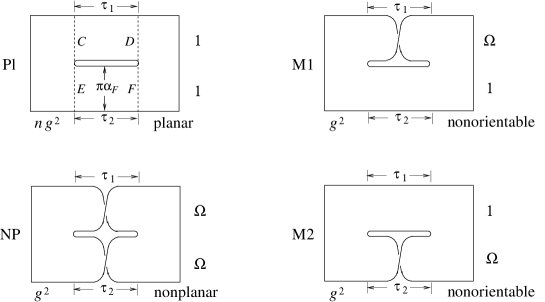
which we call planar (P), nonorientable (or Möbius) (M1 and M2) and nonplanar (NP) diagrams, respectively. To those the following four LPP vertices correspond:

$$\,\langle\tilde{V}(1,\!2;\mathchar 28956\relax_{1},\!\mathchar 28956\relax_{2})|\,={1\over 4}\bigl{\{}n\left<v_{\rm P}(\mathchar 28956\relax_{1},\!\mathchar 28956\relax_{2})\right|+\left<v_{\rm M1}(\mathchar 28956\relax_{1},\!\mathchar 28956\relax_{2})\right|+\left<v_{\rm M2}(\mathchar 28956\relax_{1},\!\mathchar 28956\relax_{2})\right|+\left<v_{\rm NP}(\mathchar 28956\relax_{1},\!\mathchar 28956\relax_{2})\right|\bigr{\}}\prod_{r=1}^{2}\!\mathchar 28933\relax^{(r)}$$ (2.16)

where the factor $n$ in front of $\left<v_{\rm P}\right|$ has come from the inner endpoint loop carrying Chan-Paton index in the planar diagram.

We take the external open string states to be on-shell tachyon states

$${\left|\mathchar 28937\relax\right>}_{r}=\,|\mathchar 28967\relax^{0}(k_{r})\rangle\,_{r}={\hbox{$\left[\vbox to0.0pt{}\right.\n@space$}}c(w_{r})\,e^{ik_{r}\cdot X^{(r)}(w_{r})}\,{\hbox{$\left]\vbox to0.0pt{}\right.\n@space$}}_{w_{r}=0}\left|0\right>_{r}\qquad\left(k_{r}^{2}=2\right).$$ (2.17)

Then, the one-loop effective action (2.9) with Eq. (2.16) substituted, yields the following one-loop 2-point tachyon amplitudes

$$\left\{\,{\cal A}_{\rm P}+{\cal A}_{\rm M1}+{\cal A}_{\rm M2}+{\cal A}_{\rm NP}\,\right\}\mathchar 28942\relax_{k_{1}{+}k_{2}}$$

$$=2i\cdot{g^{2}\over 4}\int_{0}^{\infty}d\mathchar 28956\relax_{1}d\mathchar 28956\relax_{2}\bigl{\{}\,n\left<v_{\rm P}(\mathchar 28956\relax_{1},\mathchar 28956\relax_{2})\right|+\left<v_{\rm M1}(\mathchar 28956\relax_{1},\mathchar 28956\relax_{2})\right|+\left<v_{\rm M2}(\mathchar 28956\relax_{1},\mathchar 28956\relax_{2})\right|$$

$$\hskip 100.00015pt+\left<v_{\rm NP}(\mathchar 28956\relax_{1},\mathchar 28956\relax_{2})\right|\,\bigr{\}}\,b_{\mathchar 28956\relax_{1}}b_{\mathchar 28956\relax_{2}}\,|\mathchar 28967\relax^{0}(k_{2})\rangle\,_{2}\,|\mathchar 28967\relax^{0}(k_{1})\rangle\,_{1},$$ (2.18)

with an abbreviation $\mathchar 28942\relax_{k_{1}{+}k_{2}}\equiv(2\mathchar 28953\relax)^{d}\mathchar 28942\relax^{d}(k_{1}+k_{2})$, where the individual amplitude is evaluated by the CFT on the corresponding torus $J=$ P, M1, M2, NP:

$$\left<v_{J}(\mathchar 28956\relax_{1},\mathchar 28956\relax_{2})\right|\,b_{\mathchar 28956\relax_{1}}b_{\mathchar 28956\relax_{2}}\,|\mathchar 28967\relax^{0}(k_{2})\rangle\,_{2}\,|\mathchar 28967\relax^{0}(k_{1})\rangle\,_{1}=\left<b_{\mathchar 28956\relax_{1}}b_{\mathchar 28956\relax_{2}}\,c(Z_{2})e^{ik_{2}\cdot X(Z_{2})}c(Z_{1})e^{ik_{1}\cdot X(Z_{1})}\right>_{J}.$$ (2.19)

Here we note two points. First, the RHS is generally multiplied by a factor

$$\prod_{r=1,2}\left({du\over dw_{r}}\right)_{u=Z_{r}}^{{k_{r}^{2}\over 2}-1}$$ (2.20)

which is associated with the conformal mapping of the operators $c(w_{r})e^{ik_{r}\cdot X(w_{r})}$ from the unit disk $w_{r}$ to the torus $u$ plane and $Z_{r}=u(w_{r}{=}0)$ are the positions of punctures on the torus representing the external strings. But here the factor (2.20) is 1 since the conformal weights $(k_{r}^{2}/2)-1$ are zero for the on-shell tachyons. Secondly, this Eq. (2.19) determines the CFT correlation functions on the RHS including their signs and weights. This constitutes the content of GGRT;[8, 13] namely, the loop level LPP vertex $\left<v_{J}\right|$ with $J=$ P, NO (M1 and M2), NP are already defined above as glued vertices of the two tree level LPP vertices $\left<v_{3}^{\rm o}\right|$ by Eq. (2.15) with (2.16). So these torus correlation functions are already fixed including their coefficients. We defer the explicit evaluation of these correlation functions until §5.

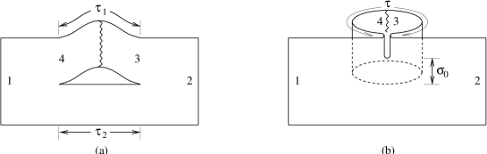
Here we first consider the nonplanar diagram NP, for which the two intermediate strings are both twisted. The amplitude ${\cal A}_{\rm NP}$ corresponding to this diagram alone does not give the full nonplanar amplitude correctly. Indeed, this can easily be seen if we redraw the diagram NP in the form as depicted in the diagram (a) in Fig. 2.

Fig. 2: (a) Loop diagram equivalent to the nonplanar diagram NP in Fig. 1. (b) A tree nonplanar diagram obtained by using the $U$ vertex twice.

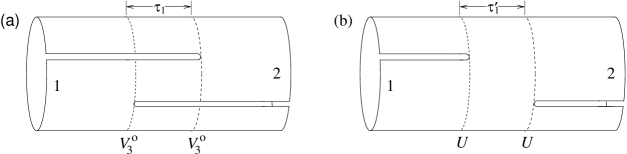
So it can cover only the $\mathchar 28956\relax_{1}>0$ part of the full nonplanar amplitude, and the remaining $0>\mathchar 28956\relax_{1}(=-\mathchar 28956\relax^{\prime}_{1})$ part is supplied by the ‘tree’ diagram given by using the open-closed transition vertex $U$ twice as drawn in the diagram (b) in Fig. 2.[14] The amplitude for this $UU$ diagram is given by

$${\cal A}_{UU}\mathchar 28942\relax_{k_{1}{+}k_{2}} = {1\over 2!}\cdot 2\left(x_{u}g\right)^{2}\,\langle U(1,A^{{\rm c}})|\,\mathop{\vbox{\halign{#\cr\kern 1.72218pt\cr$\hbox{$\hskip 8.8889pt\vrule height=7.31946pt,width=0.29999pt,depth=-0.66708pt\kern-0.29999pt\vrule height=7.31946pt,width=116.24487pt,depth=-7.01947pt\kern-0.29999pt\vrule height=7.31946pt,width=0.29999pt,depth=-0.66708pt$\hss}$\crcr\kern 1.72218pt\nointerlineskip\cr\hbox{$\displaystyle{}{\left|\mathchar 28936\relax\right>}{{}_{A^{{\mathrm{c}}}}\,|\mathchar 28967\relax^{0}(k_{1})\rangle\,_{1}\,\langle U(2,B^{{\mathrm{c}}})|\,}{\left|\mathchar 28936\relax\right>}_{B^{{\mathrm{c}}}}$}\crcr}}}\limits\,|\mathchar 28967\relax^{0}(k_{2})\rangle\,_{2}$$ (2.23)

$$= x_{u}^{2}g^{2}\int d\mathchar 28956\relax_{1}{d\mathchar 28955\relax_{1}\over 2\mathchar 28953\relax}\left<v_{UU}(\mathchar 28956\relax_{1},\mathchar 28955\relax_{1})\right|\,b_{0}\bar{b}_{0}\,\,|\mathchar 28967\relax^{0}(k_{2})\rangle\,_{2}\,|\mathchar 28967\relax^{0}(k_{1})\rangle\,_{1},$$ (2.24)

where the Wick contraction gives the closed string propagator

$$\mathop{\vbox{\halign{#\cr\kern 1.72218pt\cr$\hbox{$\hskip 40.54172pt\vrule height=7.31946pt,width=0.29999pt,depth=-0.66708pt\kern-0.29999pt\vrule height=7.31946pt,width=55.38145pt,depth=-7.01947pt\kern-0.29999pt\vrule height=7.31946pt,width=0.29999pt,depth=-0.66708pt$\hss}$\crcr\kern 1.72218pt\nointerlineskip\cr\hbox{$\displaystyle{{{(b_{0}^{-}{\mathcal{P}})}^{(A^{\mathrm{c}})}}}{\left|\mathchar 28936\relax\right>}{{}_{A^{{\mathrm{c}}}}{{(b_{0}^{-}{\mathcal{P}})}^{(B^{\mathrm{c}})}}}{\left|\mathchar 28936\relax\right>}_{B^{{\mathrm{c}}}}$}\crcr}}}\limits=\left({b_{0}\bar{b}_{0}\over L_{0}+\bar{L}_{0}}\right)^{(B^{{\mathrm{c}}})}{\mathcal{P}}^{(B^{{\mathrm{c}}})}\left|R^{\mathrm{c}}(A^{\mathrm{c}}\!,B^{\mathrm{c}})\right\rangle$$ (2.27)

$$\quad=\int d\mathchar 28956\relax_{1}{d\mathchar 28955\relax_{1}\over 2\mathchar 28953\relax}e^{-(L_{0}+\bar{L}_{0})\mathchar 28956\relax_{1}}e^{-i\mathchar 28955\relax_{1}(L_{0}-\bar{L}_{0})}\,b_{0}\bar{b}_{0}\,\left|R^{\rm c}(A^{\rm c}\!,B^{\rm c})\right\rangle$$ (2.28)

and the following glued LPP vertex has been defined:

$$\left<v_{UU}(\mathchar 28956\relax_{1},\mathchar 28955\relax_{1})\right|={\,\langle u(1,A^{\rm c})|\,}{\,\langle u(2,B^{\rm c})|\,}e^{-(L_{0}+\bar{L}_{0})\mathchar 28956\relax_{1}}e^{-i\mathchar 28955\relax_{1}(L_{0}-\bar{L}_{0})}\left|R^{\rm c}(A^{\rm c}\!,B^{\rm c})\right\rangle.$$ (2.29)

Again the amplitude is evaluated by referring to the CFT on the torus:

$$\left<v_{UU}(\mathchar 28956\relax_{1},\mathchar 28955\relax_{1})\right|\,b_{0}\bar{b}_{0}\,\,|\mathchar 28967\relax^{0}(k_{2})\rangle\,_{2}\,|\mathchar 28967\relax^{0}(k_{1})\rangle\,_{1}=\left\langle\,b_{0}\bar{b}_{0}\,c(Z_{2})e^{ik_{2}\cdot X(Z_{2})}c(Z_{1})e^{ik_{1}\cdot X(Z_{1})}\right>_{UU}.$$ (2.30)

The amplitudes ${\cal A}_{\rm NP}$ in Eq. (2.18) and ${\cal A}_{UU}$ in Eq. (2.24) should smoothly connect with each other at $\mathchar 28956\relax_{1}=0$ to reproduce the correct nonplanar amplitude, and this condition will determine the coupling constant $x_{u}$, as we shall obtain later.

Next consider the two nonorientable diagrams, M1 and M2 terms in Fig. 1. These two diagrams alone do not give the full nonorientable amplitude, again. Indeed, the two diagrams do not connect with each other at the moduli $\mathchar 28956\relax_{1}=0$, so that another diagram should exist which interconnects these two configurations at $\mathchar 28956\relax_{1}=0$. Such a diagram is just given by the ‘tree’ diagram drawn in Fig. 3 which is obtained by using the $V_{\propto}$ vertex.

Fig. 3: Tree diagram given by $V_{\propto}$ vertex which fill in the gap between the two configurations at $\mathchar 28956\relax_{1}=0$ of the nonorientable diagrams M1 and M2 in Fig. 1.

Clearly the configuration of this diagram coincides at $\mathchar 28955\relax_{2}=\mathchar 28953\relax\mathchar 28939\relax_{1}$ (and $\mathchar 28955\relax_{1}=\mathchar 28953\relax\mathchar 28939\relax_{F}$) with that of the M1 diagram at $\mathchar 28956\relax_{1}=0$, and at $\mathchar 28955\relax_{1}=0$ (and $\mathchar 28955\relax_{2}=\mathchar 28953\relax\mathchar 28939\relax_{F}$) with that of the M2 diagram at $\mathchar 28956\relax_{1}=0$. The amplitude ${\cal A}_{V\!{\propto}}$ of this diagram is proportional to $x_{\propto}$, and so the smooth connection condition for these amplitudes will determine $x_{\propto}$ as we shall see later. The amplitude ${\cal A}_{V\!{\propto}}$ is given by

$${\cal A}_{V\!{\propto}}\mathchar 28942\relax_{k_{1}{+}k_{2}} = 2\cdot x_{\propto}{g^{2}\over 2}\,\,\langle V_{\propto}(1,2)|\,\,|\mathchar 28967\relax^{0}(k_{2})\rangle\,_{2}\,|\mathchar 28967\relax^{0}(k_{1})\rangle\,_{1}$$ (2.31)

$$= x_{\propto}g^{2}\int d\mathchar 28955\relax_{1}d\mathchar 28955\relax_{2}\,\,\langle v_{\propto}(1,2;\mathchar 28955\relax_{1},\mathchar 28955\relax_{2})|\,\,b_{\mathchar 28955\relax_{1}}b_{\mathchar 28955\relax_{2}}\,|\mathchar 28967\relax^{0}(k_{2})\rangle\,_{2}\,|\mathchar 28967\relax^{0}(k_{1})\rangle\,_{1}$$

$$= x_{\propto}g^{2}\int d\mathchar 28955\relax_{1}d\mathchar 28955\relax_{2}\,\left\langle b_{\mathchar 28955\relax_{1}}b_{\mathchar 28955\relax_{2}}\,c(Z_{2})e^{ik_{2}\cdot X(Z_{2})}c(Z_{1})e^{ik_{1}\cdot X(Z_{1})}\right>_{V_{\propto}}.\hskip 30.00005pt$$

Finally, we note that the planar diagram in Fig. 1 as $\mathchar 28956\relax_{1}\rightarrow 0$ and the above diagram of $V_{\propto}$ vertex as $\mathchar 28955\relax_{1}-\mathchar 28955\relax_{2}\rightarrow 0$, both have singularities owing to the closed tachyon and dilaton vanishing into vacuum. As is shown in Fig. 4,

Fig. 4: Singular configurations for the planar diagram and $V_{\propto}$ diagram.

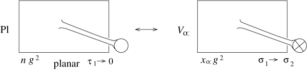
this is almost the same situation as what we have encountered in the disk and $RP^{2}$ amplitudes for closed tachyon 2-point function in the previous paper I. The former planar amplitude is proportional to $ng^{2}$ and the latter $V_{\propto}$ amplitude to $x_{\propto}$. The condition for the dilaton contributions to cancel between the two amplitudes will determine $n$ of $SO(n)$, as we shall explicitly see later.

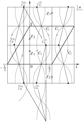
3 Conformal mapping of $\mathchar 28954\relax$ plane to torus

In order to calculate these amplitudes in Eqs. (2.18), (2.24) and (2.31), we need conformal mapping of the usual unit disk $\left|w_{r}\right|\leq 1$ of participating string $r$ to the torus for each case. The string world sheets of the ‘light-cone type’ diagrams like Figs. 1, 2 etc, are called $\mathchar 28954\relax$ plane, on which the complex coordinate $\mathchar 28954\relax=\mathchar 28956\relax+i\mathchar 28955\relax$ is identified with $\mathchar 28954\relax=\mathchar 28939\relax_{r}\mathchar 28954\relax_{r}+i\mathchar 28940\relax_{r}$ ($\mathchar 28940\relax_{r}$: a real constant) in each string $r$ strip (Re$\mathchar 28954\relax_{r}\leq 0$), where $\mathchar 28954\relax_{r}=\mathchar 28956\relax_{r}+i\mathchar 28955\relax_{r}$ is the image of the unit disk $\left|w_{r}\right|\leq 1$ of string $r$ by a simple (conformal) mapping $\mathchar 28954\relax_{r}=\ln w_{r}$. Therefore we have only to know the conformal mapping of the $\mathchar 28954\relax$ plane to the torus for each case.

The conformal mapping of the $\mathchar 28954\relax$ plane to the torus $u$ plane with periods 1 and $\mathchar 28956\relax$ is generically given by the following (generalized) Mandelstam mapping:[15, 12, 16]

$$\mathchar 28954\relax(u)=\sum_{r=1,2}\mathchar 28939\relax_{r}\ln\mathchar 28963\relax_{1}(u-Z_{r}|\mathchar 28956\relax)+Au$$ (3.1)

where $\mathchar 28963\relax_{i}(\mathchar 28951\relax|\mathchar 28956\relax)$ $(i=1,\cdots,4)$ are Jacobi $\mathchar 28963\relax$ functions with periods $1$ and $\mathchar 28956\relax$. This $\mathchar 28954\relax$ satisfies a quasi-periodicity

$$\mathchar 28954\relax(u+m\mathchar 28956\relax+n)-\mathchar 28954\relax(u)=2\mathchar 28953\relax im\sum_{r=1,2}\mathchar 28939\relax_{r}Z_{r}+A(m\mathchar 28956\relax+n).$$ (3.2)

The derivative $d\mathchar 28954\relax/du$ is truly a doubly periodic function, or elliptic function,[17] which is analytic except for the poles at $u=Z_{r}$ ($r=1,2$):

$$\frac{d\mathchar 28954\relax}{du}=\sum_{r=1,2}\mathchar 28939\relax_{r}g_{1}(u-Z_{r}|\mathchar 28956\relax)+A,$$ (3.3)

where $g_{i}$ is the logarithmic derivative of the Jacobi $\mathchar 28963\relax$ function:

$$g_{i}(\mathchar 28951\relax|\mathchar 28956\relax)\equiv{\mathchar 28963\relax^{\prime}_{i}(\mathchar 28951\relax|\mathchar 28956\relax)\over\mathchar 28963\relax_{i}(\mathchar 28951\relax|\mathchar 28956\relax)},\qquad\mathchar 28963\relax^{\prime}_{i}(\mathchar 28951\relax|\mathchar 28956\relax)\equiv{\partial\mathchar 28963\relax_{i}(\mathchar 28951\relax|\mathchar 28956\relax)\over\partial\mathchar 28951\relax}.$$ (3.4)

$Z_{r}$ corresponds to the image of the external string $r$ at $\mathchar 28956\relax_{r}=-\infty$ ($w_{r}=0$). Two interaction points $z_{0}^{(i)}$ $(i=1,\,2)$ are given by the zeros of this function:

$$\frac{d\mathchar 28954\relax}{du}(z_{0}^{(i)})=0\ \ \ \Rightarrow\ \ \ \sum_{r=1,2}\mathchar 28939\relax_{r}g_{1}(z_{0}^{(i)}-Z_{r}|\mathchar 28956\relax)+A=0.$$ (3.5)

By a general property of elliptic functions,[17] a sum rule holds:

$$Z_{1}+Z_{2}=z_{0}^{(1)}+z_{0}^{(2)}\ (\hbox{mod periods }1\ \hbox{and}\ \mathchar 28956\relax)$$ (3.6)

We now examine the conformal mappings for the cases of planar, nonorientable, nonplanar, $V_{\propto}$ and $UU$ diagrams, separately, and will find relations which determine the torus moduli $\mathchar 28956\relax$, the parameter $A$ and interaction points $z_{0}^{(i)}$ in terms of the string length and the moduli parameters of the $\mathchar 28954\relax$ plane.

3.1 Planar diagram (P)

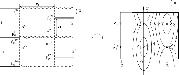
The mapping for the planar diagram case is drawn in Fig. 5.

Fig. 5: Conformal mapping of planar diagram $\mathchar 28954\relax$ plane to a torus $u$ plane. In the $\mathchar 28954\relax$ plane, the edge curve $a$-$b$ of string $E$ is identified with the curve $a^{\prime}$-$b^{\prime}$ of string $F$, which are mapped to the bottom and top lines $a$-$b$ and $a^{\prime}$-$b^{\prime}$ on the $u$ plane, respectively.

In this case the period $\mathchar 28956\relax$ is purely imaginary and denoted by ${\tilde{\mathchar 28956\relax}}$, and the mapping of this Fig. 5 is given by the above Mandelstam mapping (3.1) with $\mathchar 28956\relax$ replaced by ${\tilde{\mathchar 28956\relax}}$. The interaction points $\mathchar 28954\relax_{0}^{(i)}$ in the $\mathchar 28954\relax$ plane are mapped to $z_{0}^{(i)}$ in the $u$ plane. By using the shift invariance on the torus plane and the sum rule (3.6), we can parametrize the positions of strings (punctures) and interaction points by two real parameters $x$ and $y$ as

$$\cases{Z_{1}={\tilde{\mathchar 28956\relax}}\left(\frac{1}{2}-x\right)\cr Z_{2}={\tilde{\mathchar 28956\relax}}\left(\frac{1}{2}+x\right)\cr},\qquad\cases{z_{0}^{(1)}=\frac{1}{2}+{\tilde{\mathchar 28956\relax}}\left(\frac{1}{2}-y\right)\cr z_{0}^{(2)}=\frac{1}{2}+{\tilde{\mathchar 28956\relax}}\left(\frac{1}{2}+y\right)\cr}.$$ (3.7)

By the help of the periodicity (3.2), we can determine the parameters $A$ and $x$ as follows. First, taking $u+1=z_{0}^{(i)}$, for instance, we have $u=\hat{z}_{0}^{(i)}$ and then $\mathchar 28954\relax(u+1)=\mathchar 28954\relax_{0}^{(i)}$ and $\mathchar 28954\relax(u)=\mathchar 28954\relax_{0}^{(i)*}$, so that

$$\mathchar 28954\relax(u+1)-\mathchar 28954\relax(u)=A=\mathchar 28954\relax_{0}^{(i)}-\mathchar 28954\relax_{0}^{(i)*}=2\mathchar 28953\relax i\mathchar 28939\relax_{F}\quad\Rightarrow\quad A=2\mathchar 28953\relax i\mathchar 28939\relax_{F}\,.$$ (3.8)

Next, note that the bottom line ${\rm Im}u=0$ and the top line ${\rm Im}u=\left|{\tilde{\mathchar 28956\relax}}\right|$ with $0\leq{\rm Re}u\leq 1/2$, are mapped to the wavy curves $a$-$b$ and $a^{\prime}$-$b^{\prime}$ of strings $E$ and $F$ on the $\mathchar 28954\relax$ plane in Fig. 5. Therefore we have

$$\mathchar 28956\relax_{1}-\mathchar 28956\relax_{2}=\mathchar 28954\relax(u+{\tilde{\mathchar 28956\relax}})-\mathchar 28954\relax(u)=2\mathchar 28953\relax i\mathchar 28939\relax_{1}(Z_{1}-Z_{2})+A{\tilde{\mathchar 28956\relax}}$$

$$\qquad\Rightarrow\quad\frac{\mathchar 28956\relax_{1}}{\mathchar 28939\relax_{1}}-\frac{\mathchar 28956\relax_{2}}{\mathchar 28939\relax_{1}}=2\mathchar 28953\relax i{\tilde{\mathchar 28956\relax}}\,\left(\frac{\mathchar 28939\relax_{F}}{\mathchar 28939\relax_{1}}-2x\right)\,.$$ (3.9)

The time length $\mathchar 28956\relax_{1}$ of the intermediate C-D propagator can be connected to the torus parameter ${\tilde{\mathchar 28956\relax}}$ as follows:

$$\mathchar 28956\relax_{1} = \mathchar 28954\relax_{0}^{(2)}-\mathchar 28954\relax_{0}^{(1)}=\mathchar 28954\relax(z_{0}^{(2)})-\mathchar 28954\relax(z_{0}^{(1)})=2\mathchar 28939\relax_{1}\ln\frac{\mathchar 28963\relax_{1}(z_{0}^{(1)}-Z_{2}|{\tilde{\mathchar 28956\relax}})}{\mathchar 28963\relax_{1}(z_{0}^{(1)}-Z_{1}|{\tilde{\mathchar 28956\relax}})}+A(z_{0}^{(2)}-z_{0}^{(1)})$$ (3.10)

$$\qquad\Rightarrow\quad\frac{\mathchar 28956\relax_{1}}{\mathchar 28939\relax_{1}}=2\ln\frac{\mathchar 28963\relax_{2}({\tilde{\mathchar 28956\relax}}(x+y)|{\tilde{\mathchar 28956\relax}})}{\mathchar 28963\relax_{2}({\tilde{\mathchar 28956\relax}}(x-y)|{\tilde{\mathchar 28956\relax}})}+4\mathchar 28953\relax i\frac{\mathchar 28939\relax_{F}}{\mathchar 28939\relax_{1}}{\tilde{\mathchar 28956\relax}}y\,.$$

The Eq. (3.5) determining the interaction points, or $y$, now reads

$$g_{2}({\tilde{\mathchar 28956\relax}}(x+y)|{\tilde{\mathchar 28956\relax}})+g_{2}({\tilde{\mathchar 28956\relax}}(x-y)|{\tilde{\mathchar 28956\relax}})=-2\mathchar 28953\relax i\frac{\mathchar 28939\relax_{F}}{\mathchar 28939\relax_{1}}\,,$$ (3.11)

which is identical with the extremum condition $\partial\mathchar 28956\relax_{1}/\partial y=0$ of $\mathchar 28956\relax_{1}$ in Eq. (3.10).

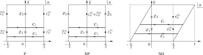
3.2 Nonorientable diagrams (M1 and M2)

The mapping of the nonorientable diagram M1 to torus is drawn in Fig. 6.

Fig. 6: Conformal mapping of the $\mathchar 28954\relax$ plane of nonorientable diagram M1 to a torus. In the $\mathchar 28954\relax$ plane, the curve $a$-$b$ is identified with the curve $a^{\prime}$-$b^{\prime}$, whose images in the $u$ plane are also shown.

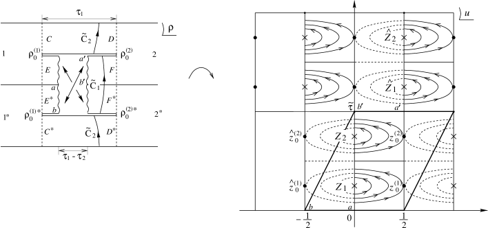
In this case the fundamental region of the torus is given as indicated in the same figure Fig. 6, and so the period $\mathchar 28956\relax$ is now given by ${\tilde{\mathchar 28956\relax}}+1/2$. Accordingly, the mapping of this Fig. 6 is given by the above Mandelstam mapping (3.1) with $\mathchar 28956\relax={\tilde{\mathchar 28956\relax}}+1/2$. We can parametrize the positions of strings (punctures) and interaction points by the same equations as Eq. (3.7) in this case also.

Similarly to the previous planar case, the periodicity (3.2) determines the parameters $A$ and $x$; from the period 1 we have the same relation as before,

$$A=2\mathchar 28953\relax i\mathchar 28939\relax_{F}.$$ (3.12)

Noting that two points separated by ${\tilde{\mathchar 28956\relax}}+1/2$, e.g., the points $a$ and $a^{\prime}$, on the $u$ plane correspond to those separated by $\mathchar 28956\relax_{1}-\mathchar 28956\relax_{2}+i\mathchar 28953\relax\mathchar 28939\relax_{F}$ on the $\mathchar 28954\relax$ plane as seen in Fig. 6, and using the period ${\tilde{\mathchar 28956\relax}}+\frac{1}{2}$ of $\mathchar 28954\relax(u)$, we obtain

$$\mathchar 28956\relax_{1}-\mathchar 28956\relax_{2}+i\mathchar 28953\relax\mathchar 28939\relax_{F} = =\mathchar 28954\relax(u+({\tilde{\mathchar 28956\relax}}+{\textstyle\frac{1}{2}}))-\mathchar 28954\relax(u)=2\mathchar 28953\relax i\mathchar 28939\relax_{1}(Z_{1}-Z_{2})+A({\tilde{\mathchar 28956\relax}}+{\textstyle\frac{1}{2}})$$ (3.13)

$$\Rightarrow\quad\frac{\mathchar 28956\relax_{1}}{\mathchar 28939\relax_{1}}-\frac{\mathchar 28956\relax_{2}}{\mathchar 28939\relax_{1}}=2\mathchar 28953\relax i{\tilde{\mathchar 28956\relax}}\,\left(\frac{\mathchar 28939\relax_{F}}{\mathchar 28939\relax_{1}}-2x\right)\,.$$

Equations for $\mathchar 28956\relax_{1}$ and the interaction point $y$ take the same form as those for the previous planar case aside from the period:

$$\frac{\mathchar 28956\relax_{1}}{\mathchar 28939\relax_{1}}=2\ln\frac{\mathchar 28963\relax_{2}({\tilde{\mathchar 28956\relax}}(x+y)|{\tilde{\mathchar 28956\relax}}+\frac{1}{2})}{\mathchar 28963\relax_{2}({\tilde{\mathchar 28956\relax}}(x-y)|{\tilde{\mathchar 28956\relax}}+\frac{1}{2})}+4\mathchar 28953\relax i\frac{\mathchar 28939\relax_{F}}{\mathchar 28939\relax_{1}}{\tilde{\mathchar 28956\relax}}y\,,$$ (3.14)

$$g_{2}({\tilde{\mathchar 28956\relax}}(x+y)|{\tilde{\mathchar 28956\relax}}+{\textstyle\frac{1}{2}})+g_{2}({\tilde{\mathchar 28956\relax}}(x-y)|{\tilde{\mathchar 28956\relax}}+{\textstyle\frac{1}{2}})=-2\mathchar 28953\relax i\frac{\mathchar 28939\relax_{F}}{\mathchar 28939\relax_{1}}\,.$$ (3.15)

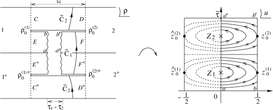
3.3 Nonplanar diagram (NP)

The mapping of the nonplanar diagram NP to torus is drawn in Fig. 7.

Fig. 7: Conformal mapping of the $\mathchar 28954\relax$ plane of nonplanar diagram NP to a torus. In the $\mathchar 28954\relax$ plane, the line connecting two crosses denotes twisting, and the curve $a$-$b$ is identified with the curve $a^{\prime}$-$b^{\prime}$, whose images in the $u$ plane are also shown.

The period $\mathchar 28956\relax$ in this case is ${\tilde{\mathchar 28956\relax}}$, the same as in planar case, and so is the Mandelstam mapping (3.1) with $\mathchar 28956\relax={\tilde{\mathchar 28956\relax}}$. However, the strings (punctures) and interaction points are placed differently from the planar case as shown in Fig. 7. So we parametrize their positions by real parameters $x$ and $y$ as

$$\cases{Z_{1}=\phantom{-\frac{1}{2}+{}}{\tilde{\mathchar 28956\relax}}\left(\frac{1}{2}-x\right)\cr Z_{2}=-\frac{1}{2}+{\tilde{\mathchar 28956\relax}}\left(\frac{1}{2}+x\right)\cr},\qquad\cases{z_{0}^{(1)}=\frac{1}{2}+{\tilde{\mathchar 28956\relax}}\left(\frac{1}{2}-y\right)\cr z_{0}^{(2)}=\phantom{\frac{1}{2}+{}}{\tilde{\mathchar 28956\relax}}\left(\frac{1}{2}+y\right)\cr}.$$ (3.16)

From the period 1 and $\mathchar 28954\relax_{0}^{(1)}-{\mathchar 28954\relax_{0}^{(1)}}^{*}=2\mathchar 28953\relax i\mathchar 28939\relax_{F}$, we again obtain the same relation as before,

$$A=2\mathchar 28953\relax i\mathchar 28939\relax_{F}.$$ (3.17)

Noting that two points separated by ${\tilde{\mathchar 28956\relax}}$, e.g., the points $a$ and $a^{\prime}$, on the $u$ plane correspond to those separated by $\mathchar 28956\relax_{1}-\mathchar 28956\relax_{2}+\mathchar 28953\relax i\mathchar 28939\relax_{1}$ on the $\mathchar 28954\relax$ plane as seen in Fig. 7, and using the period ${\tilde{\mathchar 28956\relax}}$ of $\mathchar 28954\relax(u)$, we find

$$\mathchar 28956\relax_{1}-\mathchar 28956\relax_{2}+\mathchar 28953\relax i\mathchar 28939\relax_{1} = \mathchar 28954\relax(u+{\tilde{\mathchar 28956\relax}})-\mathchar 28954\relax(u)=2\mathchar 28953\relax i\mathchar 28939\relax_{1}(Z_{1}-Z_{2})+A{\tilde{\mathchar 28956\relax}}$$ (3.18)

$$\Rightarrow\quad\frac{\mathchar 28956\relax_{1}}{\mathchar 28939\relax_{1}}-\frac{\mathchar 28956\relax_{2}}{\mathchar 28939\relax_{1}}=2\mathchar 28953\relax i{\tilde{\mathchar 28956\relax}}\,\left(\frac{\mathchar 28939\relax_{F}}{\mathchar 28939\relax_{1}}-2x\right).$$

Equations for $\mathchar 28956\relax_{1}$ and the interaction point $y$ become in this case

$$\mathchar 28956\relax_{1}+\mathchar 28953\relax i(\mathchar 28939\relax_{1}-\mathchar 28939\relax_{F}) = {\mathchar 28954\relax_{0}^{(2)}}^{*}-\mathchar 28954\relax_{0}^{(1)}=\mathchar 28954\relax(\hat{z}_{0}^{(2)})-\mathchar 28954\relax(z_{0}^{(1)})$$ (3.20)

$$= 2\mathchar 28939\relax_{1}\ln\frac{\mathchar 28963\relax_{1}(z_{0}^{(1)}-Z_{2}|{\tilde{\mathchar 28956\relax}})}{\mathchar 28963\relax_{1}(z_{0}^{(1)}-Z_{1}|{\tilde{\mathchar 28956\relax}})}+A(z_{0}^{(2)}-z_{0}^{(1)})$$

$$\Rightarrow\quad\frac{\mathchar 28956\relax_{1}}{\mathchar 28939\relax_{1}}=2\ln\frac{\mathchar 28963\relax_{1}({\tilde{\mathchar 28956\relax}}(x+y)|{\tilde{\mathchar 28956\relax}})}{\mathchar 28963\relax_{2}({\tilde{\mathchar 28956\relax}}(x-y)|{\tilde{\mathchar 28956\relax}})}+4\mathchar 28953\relax i\frac{\mathchar 28939\relax_{F}}{\mathchar 28939\relax_{1}}{\tilde{\mathchar 28956\relax}}y-\mathchar 28953\relax i\,,$$

$$g_{1}({\tilde{\mathchar 28956\relax}}(x+y)|{\tilde{\mathchar 28956\relax}})+g_{2}({\tilde{\mathchar 28956\relax}}(x-y)|{\tilde{\mathchar 28956\relax}})=-2\mathchar 28953\relax i\frac{\mathchar 28939\relax_{F}}{\mathchar 28939\relax_{1}}\,.\hskip 50.00008pt$$

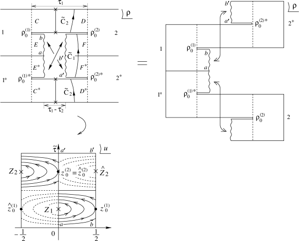
3.4 $V_{\propto}$ diagram

The diagram obtained by using $V_{\propto}$ vertex once is a tree diagram from the SFT viewpoint, but is actually a one-loop diagram from the CFT point of view. The mapping of the $V_{\propto}$ diagram to torus is drawn in Fig. 8.

Fig. 8: Conformal mapping of the $\mathchar 28954\relax$ plane of $V_{\propto}$ diagram to a torus. In the $\mathchar 28954\relax$ plane, the lines connecting two crosses denote crosscaps across which the left edge in the upper plane is identified with the right edge in the lower plane. In the $u$ plane, the parallelogram enclosed by bold solid line denotes a fundamental region of the torus corresponding to the moduli ${\tilde{\mathchar 28956\relax}}+1/2$, while that enclosed by bold dotted line denotes another choice of fundamental region corresponding to the moduli $\mathchar 28956\relax/4+1/2$ used later.

The period $\mathchar 28956\relax$ in this case is ${\tilde{\mathchar 28956\relax}}+1/2$, as is seen from the fundamental region of the torus in Fig. 8. The two interaction points in the fundamental region are

$$\cases{\tilde{z}_{0}^{(1)}=z_{0}^{(1)}+({\tilde{\mathchar 28956\relax}}+\frac{1}{2})=\hat{z}_{0}^{(2)}+1\cr z_{0}^{(2)}=\hat{z}_{0}^{(1)}+({\tilde{\mathchar 28956\relax}}+\frac{1}{2})\cr},$$ (3.21)

and we use the parametrization

$$\cases{Z_{1}={\tilde{\mathchar 28956\relax}}\left(\frac{1}{2}-x\right)\cr Z_{2}={\tilde{\mathchar 28956\relax}}\left(\frac{1}{2}+x\right)\cr},\qquad\cases{\tilde{z}_{0}^{(1)}=\frac{{\tilde{\mathchar 28956\relax}}}{2}+\left(\frac{1}{2}+y\right)\cr z_{0}^{(2)}=\frac{{\tilde{\mathchar 28956\relax}}}{2}+\left(\frac{1}{2}-y\right)\cr}.$$ (3.22)

Since $z_{0}^{(1)}+2{\tilde{\mathchar 28956\relax}}$ and $z_{0}^{(1)}$ on the $u$ plane correspond to a single point $\mathchar 28954\relax_{0}^{(1)}$ on the $\mathchar 28954\relax$ plane, we find, using the period ${\tilde{\mathchar 28956\relax}}+1/2$ of $\mathchar 28954\relax(u)$,

$$0 = \mathchar 28954\relax(z_{0}^{(1)}+2{\tilde{\mathchar 28956\relax}})-\mathchar 28954\relax(z_{0}^{(1)})=\mathchar 28954\relax(z_{0}^{(1)}+2({\tilde{\mathchar 28956\relax}}+{\textstyle\frac{1}{2}})-1)-\mathchar 28954\relax(z_{0}^{(1)})$$ (3.23)

$$= 4\mathchar 28953\relax i\mathchar 28939\relax_{1}(Z_{1}-Z_{2})+A(2({\tilde{\mathchar 28956\relax}}+{\textstyle\frac{1}{2}})-1)=-8\mathchar 28953\relax i\mathchar 28939\relax_{1}{\tilde{\mathchar 28956\relax}}x+2{\tilde{\mathchar 28956\relax}}A$$

$$\Rightarrow\quad A=4\mathchar 28953\relax i\mathchar 28939\relax_{1}x.$$

Then, $2\mathchar 28953\relax i\mathchar 28939\relax_{1}(Z_{1}-Z_{2})=-{\tilde{\mathchar 28956\relax}}A$, and hence the periodicity relation (3.2) can be rewritten as

$$\mathchar 28954\relax(u+m({\tilde{\mathchar 28956\relax}}+{\textstyle\frac{1}{2}})+n)-\mathchar 28954\relax(u)=A\left(\frac{m}{2}+n\right).$$ (3.24)

Using this periodicity and Eq. (3.21), we obtain

$$A = \mathchar 28954\relax(\tilde{z}_{0}^{(1)})-\mathchar 28954\relax(\hat{z}_{0}^{(2)})=\mathchar 28954\relax(z_{0}^{(1)}+({\tilde{\mathchar 28956\relax}}+{\textstyle\frac{1}{2}}))-\mathchar 28954\relax(\hat{z}_{0}^{(2)})$$ (3.25)

$$= \mathchar 28954\relax_{0}^{(1)}+\frac{A}{2}-{\mathchar 28954\relax_{0}^{(2)}}^{*}=i(\mathchar 28955\relax_{1}+\mathchar 28955\relax_{2})+\frac{A}{2}$$

$$\Rightarrow\quad\mathchar 28955\relax_{1}+\mathchar 28955\relax_{2}=2\mathchar 28953\relax\mathchar 28939\relax_{1}x$$

and also

$$i(\mathchar 28955\relax_{2}-\mathchar 28955\relax_{1}) = \mathchar 28954\relax(z_{0}^{(2)})-\mathchar 28954\relax(z_{0}^{(1)})=\mathchar 28954\relax(z_{0}^{(2)})-\mathchar 28954\relax(\tilde{z}_{0}^{(1)}-({\tilde{\mathchar 28956\relax}}+{\textstyle\frac{1}{2}}))$$ (3.26)

$$= \mathchar 28954\relax(z_{0}^{(2)})-\mathchar 28954\relax(\tilde{z}_{0}^{(1)})+\frac{A}{2}$$

$$= 2\mathchar 28939\relax_{1}\ln\frac{\mathchar 28963\relax_{1}(\tilde{z}_{0}^{(1)}-Z_{2}|{\tilde{\mathchar 28956\relax}}+\frac{1}{2})}{\mathchar 28963\relax_{1}(\tilde{z}_{0}^{(1)}-Z_{1}|{\tilde{\mathchar 28956\relax}}+\frac{1}{2})}+A(z_{0}^{(2)}-\tilde{z}_{0}^{(1)})+\frac{A}{2}$$

$$\Rightarrow\quad i{\mathchar 28955\relax_{2}-\mathchar 28955\relax_{1}\over\mathchar 28939\relax_{1}}=-2\ln\frac{\mathchar 28963\relax_{2}({\tilde{\mathchar 28956\relax}}x+y|{\tilde{\mathchar 28956\relax}}+\frac{1}{2})}{\mathchar 28963\relax_{2}({\tilde{\mathchar 28956\relax}}x-y|{\tilde{\mathchar 28956\relax}}+\frac{1}{2})}+2\mathchar 28953\relax ix(1-4y)\,.$$

The equation determining the interaction point $y$ is again the same as the stationarity condition $\partial(\mathchar 28955\relax_{1}-\mathchar 28955\relax_{2})/\partial y=0$:

$$g_{2}({\tilde{\mathchar 28956\relax}}x+y|{\tilde{\mathchar 28956\relax}}+{\textstyle\frac{1}{2}})+g_{2}({\tilde{\mathchar 28956\relax}}x-y|{\tilde{\mathchar 28956\relax}}+{\textstyle\frac{1}{2}})=-4\mathchar 28953\relax ix\,.$$ (3.27)

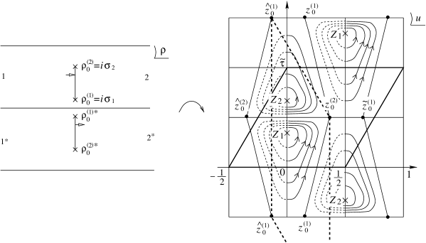
3.5 $UU$ diagram

The diagram obtained by using $U$ vertex twice is again a tree diagram from the SFT viewpoint but is a one-loop diagram from the CFT viewpoint. The mapping of the $UU$ diagram to torus is drawn in Fig. 9.

Fig. 9: Conformal mapping of the $\mathchar 28954\relax$ plane of $UU$ diagram to a torus.

The period $\mathchar 28956\relax$ in this case is ${\tilde{\mathchar 28956\relax}}$, the same as in planar case, and we parametrize the positions of punctures and interaction points as

$$\cases{Z_{1}=\phantom{\frac{1}{2}+{}}{\tilde{\mathchar 28956\relax}}\left(\frac{1}{2}-x\right)\cr Z_{2}=-\frac{1}{2}+{\tilde{\mathchar 28956\relax}}\left(\frac{1}{2}+x\right)\cr},\qquad\cases{z_{0}^{(1)}=\phantom{\frac{1}{2}+{}}{\tilde{\mathchar 28956\relax}}\left(\frac{1}{2}+y\right)\cr z_{0}^{(2)}=\frac{1}{2}+{\tilde{\mathchar 28956\relax}}\left(\frac{1}{2}-y\right)\cr}.$$ (3.28)

From periods ${\tilde{\mathchar 28956\relax}}$ and 1, we obtain

$$\mathchar 28953\relax i\mathchar 28939\relax_{1} = \mathchar 28954\relax(z_{0}^{(1)})-\mathchar 28954\relax(z_{0}^{(1)}-{\tilde{\mathchar 28956\relax}})=2\mathchar 28953\relax i\mathchar 28939\relax_{1}(Z_{1}-Z_{2})+A{\tilde{\mathchar 28956\relax}}$$ (3.29)

$$\Rightarrow \quad A=4\mathchar 28953\relax i\mathchar 28939\relax_{1}x\,,$$

$$2i\mathchar 28955\relax_{1} = \mathchar 28954\relax(z_{0}^{(2)})-\mathchar 28954\relax(\hat{z}_{0}^{(2)})=\mathchar 28954\relax(\hat{z}_{0}^{(2)}+1)-\mathchar 28954\relax(\hat{z}_{0}^{(2)})=A$$ (3.30)

$$\Rightarrow \quad\mathchar 28955\relax_{1}=2\mathchar 28953\relax\mathchar 28939\relax_{1}x\,.$$

As for the relation between $\mathchar 28956\relax_{1}$ and the torus moduli ${\tilde{\mathchar 28956\relax}}$, we find

$$\mathchar 28956\relax_{1}+i\mathchar 28955\relax_{1} = \mathchar 28954\relax(z_{0}^{(2)})-\mathchar 28954\relax(z_{0}^{(1)}-{\tilde{\mathchar 28956\relax}})=\mathchar 28954\relax(z_{0}^{(2)})-\mathchar 28954\relax(z_{0}^{(1)})+\mathchar 28953\relax i\mathchar 28939\relax_{1}$$ (3.31)

$$= 2\mathchar 28939\relax_{1}\ln\frac{\mathchar 28963\relax_{1}(z_{0}^{(1)}-Z_{2}|{\tilde{\mathchar 28956\relax}})}{\mathchar 28963\relax_{1}(z_{0}^{(1)}-Z_{1}|{\tilde{\mathchar 28956\relax}})}+A(z_{0}^{(2)}-z_{0}^{(1)})+\mathchar 28953\relax i\mathchar 28939\relax_{1}$$

$$\Rightarrow\quad\frac{\mathchar 28956\relax_{1}}{\mathchar 28939\relax_{1}}=-2\ln\frac{\mathchar 28963\relax_{1}({\tilde{\mathchar 28956\relax}}(x+y)|{\tilde{\mathchar 28956\relax}})}{\mathchar 28963\relax_{2}({\tilde{\mathchar 28956\relax}}(x-y)|{\tilde{\mathchar 28956\relax}})}-8\mathchar 28953\relax ix{\tilde{\mathchar 28956\relax}}y+\mathchar 28953\relax i\,.$$

Stationarity $\partial\mathchar 28956\relax_{1}/\partial y=0$ determines the interaction point $y$:

$$g_{1}({\tilde{\mathchar 28956\relax}}(x+y)|{\tilde{\mathchar 28956\relax}})+g_{2}({\tilde{\mathchar 28956\relax}}(x-y)|{\tilde{\mathchar 28956\relax}})=-4\mathchar 28953\relax ix\,.$$ (3.32)

4 Jacobian

In the explicit computation of the amplitudes below, we will need to make change of the variables from the moduli parameters on the $\mathchar 28954\relax$ plane to the torus moduli $\mathchar 28956\relax$ and $x$. Here we compute the Jacobian for this change of variables, for each case of the diagrams.

4.1 general

Since the Jacobi $\mathchar 28963\relax$ functions satisfy

$${\partial\mathchar 28963\relax_{i}(\mathchar 28951\relax|\mathchar 28956\relax)\over\partial\mathchar 28956\relax}=-{i\over 4\mathchar 28953\relax}{\partial^{2}\mathchar 28963\relax_{i}(\mathchar 28951\relax|\mathchar 28956\relax)\over\partial\mathchar 28951\relax^{2}}\,,$$ (4.1)

we have the following relation using $g_{i}(\mathchar 28951\relax|\mathchar 28956\relax)$ defined in Eq. (3.4):

$${\partial\over\partial\mathchar 28956\relax}\ln\mathchar 28963\relax_{i}(\mathchar 28951\relax|\mathchar 28956\relax)=-{i\over 4\mathchar 28953\relax}{\mathchar 28963\relax^{\prime\prime}_{i}\over\mathchar 28963\relax_{i}}(\mathchar 28951\relax|\mathchar 28956\relax)=-{i\over 4\mathchar 28953\relax}(g^{\prime}_{i}+g^{2}_{i})(\mathchar 28951\relax|\mathchar 28956\relax)\,.$$ (4.2)

Using this equation, we can $\mathchar 28956\relax$-differentiate Eq.(3.1) with $u$ generally dependent of $\mathchar 28956\relax$:

$$\frac{\partial\mathchar 28954\relax(u)}{\partial\mathchar 28956\relax}=\frac{\partial u}{\partial\mathchar 28956\relax}\frac{d\mathchar 28954\relax}{du}-\sum_{r=1,2}\mathchar 28939\relax_{r}\frac{\partial Z_{r}}{\partial\mathchar 28956\relax}g_{1}(u-Z_{r})-\sum_{r=1,2}\frac{i\mathchar 28939\relax_{r}}{4\mathchar 28953\relax}\left(g_{1}^{\prime}(u-Z_{r})+{g_{1}}^{2}(u-Z_{r})\right),$$ (4.3)

where the period $\mathchar 28956\relax$ has been omitted for brevity. When $u=z_{0}^{(i)}$ (in the fundamental region), $d\mathchar 28954\relax/du(z_{0}^{(i)})=0$ because of Eq. (3.5) and we have

$$\frac{\partial\mathchar 28954\relax(z_{0}^{(i)})}{\partial\mathchar 28956\relax}=-\sum_{r=1,2}\mathchar 28939\relax_{r}\frac{\partial Z_{r}}{\partial\mathchar 28956\relax}g_{1}(z_{0}^{(i)}-Z_{r})-\sum_{r=1,2}\frac{i\mathchar 28939\relax_{r}}{4\mathchar 28953\relax}\left(g_{1}^{\prime}(z_{0}^{(i)}-Z_{r})+{g_{1}}^{2}(z_{0}^{(i)}-Z_{r})\right).$$ (4.4)

Using further the identities

$$\mathchar 28963\relax_{1}(z_{0}^{(2)}-Z_{1})=\mathchar 28963\relax_{1}(z_{0}^{(1)}-Z_{2})\qquad\hbox{when}\quad Z_{1}+Z_{2}+1=z_{0}^{(1)}+z_{0}^{(2)}$$

$$\ \ \Rightarrow\ \ g_{1}(z_{0}^{(2)}-Z_{1})=-g_{1}(z_{0}^{(1)}-Z_{2}),\quad g_{1}^{\prime}(z_{0}^{(2)}-Z_{1})=g_{1}^{\prime}(z_{0}^{(1)}-Z_{2}),\hskip 20.00003pt$$ (4.5)

where $z_{0}^{(1)}$ is understood to be $\tilde{z}_{0}^{(1)}$ for the $V_{\propto}$ case, we obtain

$$\frac{\partial}{\partial\mathchar 28956\relax}\left(\mathchar 28954\relax(z_{0}^{(2)})-\mathchar 28954\relax(z_{0}^{(1)})\right)$$

$$=\mathchar 28939\relax_{1}\frac{\partial(Z_{1}-Z_{2})}{\partial\mathchar 28956\relax}\left(g_{1}(z_{0}^{(1)}-Z_{1})+g_{1}(z_{0}^{(1)}-Z_{2})\right)$$

$$\qquad{}+\frac{i\mathchar 28939\relax_{1}}{2\mathchar 28953\relax}\left(g_{1}^{\prime}(z_{0}^{(1)}-Z_{1})-g_{1}^{\prime}(z_{0}^{(1)}-Z_{2})+{g_{1}}^{2}(z_{0}^{(1)}-Z_{1})-{g_{1}}^{2}(z_{0}^{(1)}-Z_{2})\right)$$

$$=\frac{i\mathchar 28939\relax_{1}}{2\mathchar 28953\relax}{\hbox{$\left(\vbox to0.0pt{}\right.\n@space$}}g_{1}(z_{0}^{(1)}{-}Z_{1})+g_{1}(z_{0}^{(1)}{-}Z_{2}){\hbox{$\left)\vbox to0.0pt{}\right.\n@space$}}\left\{g_{1}(z_{0}^{(1)}{-}Z_{1})-g_{1}(z_{0}^{(1)}{-}Z_{2})-2\mathchar 28953\relax i\frac{\partial(Z_{1}{-}Z_{2})}{\partial\mathchar 28956\relax}\right\}$$

$$\qquad{}+\frac{i\mathchar 28939\relax_{1}}{2\mathchar 28953\relax}\left[\,g_{1}^{\prime}(z_{0}^{(1)}-Z_{1})-g_{1}^{\prime}(z_{0}^{(1)}-Z_{2})\,\right].$$ (4.6)

In the present case of tachyon amplitude, we shall see below that the amplitudes for P, NO (M1 and M2) and NP diagrams contain delta function factor $\mathchar 28942\relax(\mathchar 28956\relax_{1}-\mathchar 28956\relax_{2})$ (which is always the case when the external string states have no excitations of $\mathchar 28939\relax_{n}^{-}$ modes (See §7)). Then, as seen in Eqs. (3.9), (3.13) and (3.18) in those cases of P, NO (M1 and M2) and NP diagrams, $\mathchar 28956\relax_{1}=\mathchar 28956\relax_{2}$ means

$$A=2\mathchar 28953\relax i\mathchar 28939\relax_{F}=4\mathchar 28953\relax i\mathchar 28939\relax_{1}x\,,$$ (4.7)

the same expression as Eqs. (3.23) and (3.29) for the $V_{\propto}$ and $UU$ amplitude cases. Thus, for all amplitude cases, we have

$$-2\mathchar 28953\relax i\frac{\partial(Z_{1}-Z_{2})}{\partial\mathchar 28956\relax}=4\mathchar 28953\relax ix=\frac{A}{\mathchar 28939\relax_{1}}\,,$$ (4.8)

which together with Eq.(3.5) implies that the part enclosed by a curly bracket in Eq. (4.1) vanishes. Consequently we obtain

$$\frac{\partial}{\partial\mathchar 28956\relax}\left(\mathchar 28954\relax(z_{0}^{(2)})-\mathchar 28954\relax(z_{0}^{(1)})\right)=\frac{i\mathchar 28939\relax_{1}}{2\mathchar 28953\relax}\left[\,g_{1}^{\prime}(z_{0}^{(1)}-Z_{1}|\mathchar 28956\relax)-g_{1}^{\prime}(z_{0}^{(1)}-Z_{2}|\mathchar 28956\relax)\,\right].$$ (4.9)

4.2 P, NO, NP

In these cases under the condition $\mathchar 28956\relax_{1}=\mathchar 28956\relax_{2}$, remaining two free parameters are

$$\mathchar 28939\relax_{F} = 2\mathchar 28939\relax_{1}x\,,$$

$$\mathchar 28956\relax_{1} = \cases{\mathchar 28954\relax(z_{0}^{(2)})-\mathchar 28954\relax(z_{0}^{(1)})&for P, NO\cr\mathchar 28954\relax(z_{0}^{(2)})-\mathchar 28954\relax(z_{0}^{(1)})-\mathchar 28953\relax i\mathchar 28939\relax_{1}+2\mathchar 28953\relax i\mathchar 28939\relax_{1}x&for NP\cr}.$$ (4.10)

Taking account of Eq.(4.9), the Jacobian for the change of variables $(\mathchar 28956\relax_{1},\mathchar 28939\relax_{F})\ \rightarrow\ (\mathchar 28956\relax,x)$ has the form

$$d\mathchar 28956\relax_{1}d\mathchar 28939\relax_{F} = \frac{\partial(\mathchar 28956\relax_{1},\mathchar 28939\relax_{F})}{\partial(\mathchar 28956\relax,x)}d\mathchar 28956\relax dx=\frac{\partial\mathchar 28956\relax_{1}}{\partial\mathchar 28956\relax}\frac{\partial\mathchar 28939\relax_{F}}{\partial x}d\mathchar 28956\relax dx$$ (4.11)

$$= 2\mathchar 28939\relax_{1}\cdot\frac{i\mathchar 28939\relax_{1}}{2\mathchar 28953\relax}\left[\,g_{1}^{\prime}(z_{0}^{(1)}-Z_{1}|\mathchar 28956\relax)-g_{1}^{\prime}(z_{0}^{(1)}-Z_{2}|\mathchar 28956\relax)\,\right]d\mathchar 28956\relax dx.$$

Here $\mathchar 28956\relax={\tilde{\mathchar 28956\relax}}$ for P, NP and $\mathchar 28956\relax={\tilde{\mathchar 28956\relax}}+\frac{1}{2}$ for NO, but $d\mathchar 28956\relax=d{\tilde{\mathchar 28956\relax}}$ in any case. More explicitly, using Eqs. (3.7), (3.16), $g_{1}(u+1/2)=g_{2}(u)$ and $g^{\prime}_{i}(-u)=g^{\prime}_{i}(u)$,

$$d\mathchar 28956\relax_{1}d\mathchar 28939\relax_{F}=-{{i\mathchar 28939\relax_{1}}^{2}\over\mathchar 28953\relax}{\times}\cases{\displaystyle\left[\,g_{2}^{\prime}\left({\tilde{\mathchar 28956\relax}}(x+y)|{\tilde{\mathchar 28956\relax}}\right)-g_{2}^{\prime}\left({\tilde{\mathchar 28956\relax}}(x-y)|{\tilde{\mathchar 28956\relax}}\right)\,\right]d{\tilde{\mathchar 28956\relax}}dx&for P\cr\displaystyle\left[\,g_{2}^{\prime}\left({\tilde{\mathchar 28956\relax}}(x+y)|{\tilde{\mathchar 28956\relax}}+{\textstyle\frac{1}{2}}\right)-g_{2}^{\prime}\left({\tilde{\mathchar 28956\relax}}(x-y)|{\tilde{\mathchar 28956\relax}}+{\textstyle\frac{1}{2}}\right)\,\right]d{\tilde{\mathchar 28956\relax}}dx&for NO\cr\displaystyle\left[\,g_{1}^{\prime}\left({\tilde{\mathchar 28956\relax}}(x+y)|{\tilde{\mathchar 28956\relax}}\right)-g_{2}^{\prime}\left({\tilde{\mathchar 28956\relax}}(x-y)|{\tilde{\mathchar 28956\relax}}\right)\,\right]d{\tilde{\mathchar 28956\relax}}dx&for NP\cr}.$$ (4.12)

4.3 $V_{\propto}$

Two free parameters in this $V_{\propto}$ case are

$$i\mathchar 28955\relax_{+} \equiv i(\mathchar 28955\relax_{1}+\mathchar 28955\relax_{2})=2\mathchar 28953\relax i\mathchar 28939\relax_{1}x$$

$$i\mathchar 28955\relax_{-} \equiv i(\mathchar 28955\relax_{2}-\mathchar 28955\relax_{1})=\mathchar 28954\relax(z_{0}^{(2)})-\mathchar 28954\relax(\tilde{z}_{0}^{(1)})+2\mathchar 28953\relax i\mathchar 28939\relax_{1}x\,.$$ (4.13)

The Jacobian for the change of variables $(\mathchar 28955\relax_{1},\mathchar 28955\relax_{2})\ \rightarrow\ (\mathchar 28956\relax,x)$ is given by

$$d\mathchar 28955\relax_{1}d\mathchar 28955\relax_{2} = -\frac{1}{2}d\mathchar 28955\relax_{-}d\mathchar 28955\relax_{+}=\frac{1}{2}\frac{\partial(i\mathchar 28955\relax_{-},i\mathchar 28955\relax_{+})}{\partial(\mathchar 28956\relax,x)}d\mathchar 28956\relax dx=\frac{1}{2}\frac{\partial i\mathchar 28955\relax_{-}}{\partial\mathchar 28956\relax}\frac{\partial i\mathchar 28955\relax_{+}}{\partial x}d\mathchar 28956\relax dx$$ (4.14)

$$= i\mathchar 28953\relax\mathchar 28939\relax_{1}\cdot\frac{i\mathchar 28939\relax_{1}}{2\mathchar 28953\relax}\left[\,g_{1}^{\prime}(\tilde{z}_{0}^{(1)}-Z_{1}|\mathchar 28956\relax)-g_{1}^{\prime}(\tilde{z}_{0}^{(1)}-Z_{2}|\mathchar 28956\relax)\,\right]d\mathchar 28956\relax dx.$$

More explicitly, using $\mathchar 28956\relax={\tilde{\mathchar 28956\relax}}+1/2$ and Eq. (3.22),

$$d\mathchar 28955\relax_{1}d\mathchar 28955\relax_{2}=-\frac{{\mathchar 28939\relax_{1}}^{2}}{2}\left[\,g_{2}^{\prime}\left({\tilde{\mathchar 28956\relax}}x+y|{\tilde{\mathchar 28956\relax}}+{\textstyle\frac{1}{2}}\right)-g_{2}^{\prime}\left({\tilde{\mathchar 28956\relax}}x-y|{\tilde{\mathchar 28956\relax}}+{\textstyle\frac{1}{2}}\right)\,\right]d{\tilde{\mathchar 28956\relax}}dx.$$ (4.15)

4.4 $UU$

Free parameters in the $UU$ case are

$$\mathchar 28955\relax_{1} = 2\mathchar 28953\relax\mathchar 28939\relax_{1}x$$

$$\mathchar 28956\relax_{1} = \mathchar 28954\relax(z_{0}^{(2)})-\mathchar 28954\relax(z_{0}^{(1)})+\mathchar 28953\relax i\mathchar 28939\relax_{1}-2\mathchar 28953\relax i\mathchar 28939\relax_{1}x,$$ (4.16)

so that the Jacobian for the change of variables $(\mathchar 28955\relax_{1},\mathchar 28956\relax_{1})\ \rightarrow\ (\mathchar 28956\relax,x)$ reads

$$d\mathchar 28956\relax_{1}d\mathchar 28955\relax_{1} = \frac{\partial(\mathchar 28956\relax_{1},\mathchar 28955\relax_{1})}{\partial(\mathchar 28956\relax,x)}d\mathchar 28956\relax dx=\frac{\partial\mathchar 28956\relax_{1}}{\partial\mathchar 28956\relax}\frac{\partial\mathchar 28955\relax_{1}}{\partial x}d\mathchar 28956\relax dx$$ (4.17)

$$= 2\mathchar 28953\relax\mathchar 28939\relax_{1}\cdot\frac{i\mathchar 28939\relax_{1}}{2\mathchar 28953\relax}\left[\,g_{1}^{\prime}(z_{0}^{(1)}-Z_{1}|\mathchar 28956\relax)-g_{1}^{\prime}(z_{0}^{(1)}-Z_{2}|\mathchar 28956\relax)\,\right]d\mathchar 28956\relax dx.$$

More explicitly, using $\mathchar 28956\relax={\tilde{\mathchar 28956\relax}}$ and Eq. (3.28),

$$d\mathchar 28956\relax_{1}d\mathchar 28955\relax_{1}=i{\mathchar 28939\relax_{1}}^{2}\left[\,g_{1}^{\prime}({\tilde{\mathchar 28956\relax}}(x+y)|{\tilde{\mathchar 28956\relax}})-g_{2}^{\prime}({\tilde{\mathchar 28956\relax}}(x-y)|{\tilde{\mathchar 28956\relax}})\,\right]d{\tilde{\mathchar 28956\relax}}dx.$$ (4.18)

5 CFT correlation functions on the torus

5.1 Correlation functions and GGRT

To compute the CFT correlation functions on the torus, we further map the $u$ plane to the $\tilde{\mathchar 28954\relax}=-2\mathchar 28953\relax iu$ plane such that the $\tilde{\mathchar 28954\relax}=\mathchar 28956\relax+i\mathchar 28955\relax$ plane becomes of the usual open string strip with ${\rm Im}\tilde{\mathchar 28954\relax}\,({=}\mathchar 28955\relax)=0$ and $\mathchar 28953\relax$ being the open string boundaries and, therefore, the usual Fourier expansion $\mathchar 28958\relax(\tilde{\mathchar 28954\relax})=\sum_{n}\mathchar 28958\relax_{n}e^{-n\tilde{\mathchar 28954\relax}}$ can be used there for the string coordinate and ghost fields $\mathchar 28958\relax=X,b$ and $c$. Then, the CFT correlation functions can be calculated by the following formulas: for the cases of P and NP diagrams with period ${\tilde{\mathchar 28956\relax}}$,

$$\bigl{<}\,\prod_{r}{\cal O}_{r}(u_{r})\,\bigr{>}_{{\tilde{\mathchar 28956\relax}}}=(-2\mathchar 28953\relax i)^{\sum_{r}\!d_{r}}\mathop{\rm Tr}\bigl{[}(-)^{N_{\rm FP}+1}\,w^{(L_{0}-{c/24})}\,\prod_{r}{\cal O}_{r}(-2\mathchar 28953\relax iu_{r})\,\bigr{]},$$ (5.1)

and for the NO (M1 and M2) cases with period ${\tilde{\mathchar 28956\relax}}+\frac{1}{2}$,

$$\bigl{<}\,\prod_{r}{\cal O}_{r}(u_{r})\,\bigr{>}_{{\tilde{\mathchar 28956\relax}}+\frac{1}{2}}\!=(-2\mathchar 28953\relax i)^{\sum_{r}\!d_{r}}\mathop{\rm Tr}\bigl{[}\mathchar 28938\relax(-)^{N_{\rm FP}+1}w^{(L_{0}-{c/24})}\prod_{r}{\cal O}_{r}(-2\mathchar 28953\relax iu_{r})\bigr{]},$$ (5.2)

where $w\equiv e^{2\mathchar 28953\relax i{\tilde{\mathchar 28956\relax}}}$, $N_{\rm FP}$ is the ghost number operator (whose explicit expression is given shortly), $c$ is the central charge of the system, and $\mathchar 28938\relax$ is the (open string) twist operator, $\mathchar 28938\relax:u\rightarrow u+\frac{1}{2}$ $(\tilde{\mathchar 28954\relax}\rightarrow\tilde{\mathchar 28954\relax}-\mathchar 28953\relax i)$. Here we have assumed that the operators ${\cal O}_{r}$ are primary fields with conformal weights $d_{r}$, as being always the case in our computations below.

As noted before, these formulas are not mere definitions of the torus CFT correlation functions but the result of the GGRT[13] for the cases of P, NP and NO diagrams. Actually, once the period is specified, the functional form of the torus correlation function is unique but the overall normalization factor is not. GGRT determines those normalization factors also.

For the remaining $UU$ and $V_{\propto}$ cases, these formula does not give the correct normalization factor. First consider the $UU$ diagram case, in which the $\left<v_{UU}\right|$ vertex is given in Eq. (2.29) by contracting two tree level $U$ vertices by closed reflector $\left|R^{\rm c}(A^{\rm c}\!,B^{\rm c})\right\rangle$. In view of the $u$ plane in Fig. 9 in which the vertical lines represent the intermediate closed string, we note that the direction of the time evolution on the $u$ plane is not vertical but horizontal in the $UU$ diagram case. So the trace operation should be taken in the horizontal direction in this $UU$ diagram case, and the correct mapping from the $u$ plane to $\tilde{\mathchar 28954\relax}$ plane should be $\tilde{\mathchar 28954\relax}=2\mathchar 28953\relax u(i/{\tilde{\mathchar 28956\relax}})+$const. such that the image of the vertical line ${\rm Re}u={}$const., $0\leq{\rm Im}u\leq\left|{\tilde{\mathchar 28956\relax}}\right|(={\tilde{\mathchar 28956\relax}}/i)$ has the correct width $2\mathchar 28953\relax$ in $\mathchar 28955\relax={\rm Im}\tilde{\mathchar 28954\relax}$. Using this mapping and denoting $-1/{\tilde{\mathchar 28956\relax}}\equiv\mathchar 28956\relax$, the correct formula in this $UU$ case reads

$$\bigl{<}\,\prod_{r}{\cal O}_{r}(u_{r})\,\bigr{>}_{UU,\mathchar 28956\relax}=(-2\mathchar 28953\relax i\mathchar 28956\relax)^{\sum_{r}\!d_{r}}{\mathop{\rm Tr}}^{\prime}\bigl{[}(-)^{N_{\rm FP}+1}\,q^{2(L_{0}-{c/24})}\prod_{r}{\cal O}_{r}(-2\mathchar 28953\relax i\mathchar 28956\relax u_{r})\bigr{]},$$ (5.3)

where $q\equiv e^{\mathchar 28953\relax i\mathchar 28956\relax}$, and ${\mathop{\rm Tr}}^{\prime}$ means that no trace is taken over the momentum; the ‘trace’ $\mathop{\rm Tr}_{0}[\cdots]$ in the zero mode sector of $X$ is simply $\left<-k_{1}/2\right|\cdots\left|-k_{1}/2\right>$ where $k_{1}$ is the momentum of the external string 1. We emphasize again that the difference between the CFT correlation functions (5.1) and (5.3) computed vertically and horizontally, respectively, in fact appears only in their numerical coefficients and their function forms are exactly the same.

For completeness, we present here the proof for this formula (5.3). It can be proven by using the GGRT for the case of open-string loop diagram.[13] The closed string $A^{\rm c}$ can be treated essentially as a product of two open strings $A$ and $\bar{A}$, corresponding to the holomorphic and anti-holomorphic pieces. This identification is, however, slightly violated in the zero-mode sector of $X$, since there exists only a single zero-mode $x$ (or $p$) common to the holomorphic and anti-holomorphic parts. To make the identification exact, we can extend the zero mode sector such that both the holomorphic and anti-holomorphic sectors have their own zero modes $p$ and $\bar{p}$, and identify the original state $\left|p_{1}\right>$ to be $\left|p,\bar{p}\right>$ with $p+\bar{p}=p_{1}$ and $p-\bar{p}=0$. Then, taking account of $dp\,d\bar{p}=d(p+\bar{p})\,d((p-\bar{p})/2)$, we can identify the closed reflector $\left|R^{\rm c}(A^{\rm c}\!,B^{\rm c})\right\rangle$ as

$$\left|R^{\rm c}(A^{\rm c}\!,B^{\rm c})\right\rangle=(2\mathchar 28953\relax)^{d}\mathchar 28942\relax^{d}\bigl{(}{\hat{p}_{A}-{\hat{p}}_{\bar{A}}\over 2}\bigr{)}\left|R^{\rm o}(A,B)\right\rangle\left|R^{\rm o}(\bar{A},\bar{B})\right\rangle$$ (5.4)

and the vertex ${\,\langle u(1,A^{\rm c})|\,}$, for instance, becomes to have momentum conservation factor $\mathchar 28942\relax^{d}(p_{A}+\bar{p}_{A}+k_{1})$ instead of $\mathchar 28942\relax^{d}(p_{A}+k_{1})$. With this device, we now apply the GGRT[8, 13] for the open string case to the present $UU$ vertex contracted by the closed string reflector: with $\mathchar 28954\relax_{1}\equiv\mathchar 28956\relax_{1}+i\mathchar 28955\relax_{1}$,

$$\left<v_{UU}(\mathchar 28956\relax_{1},\mathchar 28955\relax_{1})\right|$$

$$\quad={\,\langle u(1,A^{\rm c})|\,}{\,\langle u(2,B^{\rm c})|\,}e^{-L_{0}\mathchar 28954\relax_{1}}e^{-\bar{L}_{0}\bar{\mathchar 28954\relax}_{1}}\left|R^{\rm c}(A^{\rm c}\!,B^{\rm c})\right\rangle$$

$$\quad=\,\langle u(\bar{A},1,A)|\,e^{-L_{0}\mathchar 28954\relax_{1}}\,\langle u(B,2,\bar{B})|\,e^{-\bar{L}_{0}\bar{\mathchar 28954\relax}_{1}}(2\mathchar 28953\relax)^{d}\mathchar 28942\relax^{d}\bigl{(}{\hat{p}_{A}-{\hat{p}}_{\bar{A}}\over 2}\bigr{)}\left|R^{\rm o}(A,B)\right\rangle\left|R^{\rm o}(\bar{A},\bar{B})\right\rangle$$

$$\quad=\,\langle u(\bar{A},1,A)|\,e^{-L_{0}\mathchar 28954\relax_{1}}\,\langle u(B,2,\bar{B})|\,\left|R^{\rm o}(A,B)\right\rangle e^{-\bar{L}_{0}\bar{\mathchar 28954\relax}_{1}}(2\mathchar 28953\relax)^{d}\mathchar 28942\relax^{d}\bigl{(}\hat{p}_{\bar{A}}+{k_{1}\over 2}\bigr{)}\left|R^{\rm o}(\bar{A},\bar{B})\right\rangle$$

$$\quad=\,\langle v(\bar{A},1,2,\bar{B})|\,e^{-\bar{L}_{0}\bar{\mathchar 28954\relax}_{1}}(2\mathchar 28953\relax)^{d}\mathchar 28942\relax^{d}\bigl{(}\hat{p}_{\bar{A}}+{p_{1}\over 2}\bigr{)}\left|R^{\rm o}(\bar{A},\bar{B})\right\rangle\,,$$ (5.5)

where we have used the momentum conservation $\,\langle u(\bar{A},1,A)|\,(\hat{p}_{A}+\hat{p}_{\bar{A}}+k_{1})=0$ in going to the third expression, and the tree level GGRT $\,\langle v(\bar{A},1,2,\bar{B})|\,=\,\langle u(\bar{A},1,A)|\,e^{-L_{0}\mathchar 28954\relax_{1}}\,\langle u(B,2,\bar{B})|\,\left|R(A,B)\right>$ in going to the last line. Since every quantities are now of open-string, we can apply the loop level GGRT proven in Ref. ? to the last expression and obtain

$$\left<v_{UU}(\mathchar 28956\relax_{1},\mathchar 28955\relax_{1})\right|\left|\mathchar 28936\relax_{2}\right>\left|\mathchar 28936\relax_{1}\right>$$

$$\qquad=\int{d^{d}{p}\over(2\mathchar 28953\relax)^{d}}\left<{p}\right|(2\mathchar 28953\relax)^{d}\mathchar 28942\relax^{d}\bigl{(}\hat{p}_{\bar{A}}+{k_{1}\over 2}\bigr{)}\mathop{\rm Tr}_{n\not=0}\bigl{[}(-)^{N_{\rm FP}+1}\,q^{2L_{0}}\prod_{i}h_{i}[\mathchar 28936\relax_{i}]\bigr{]}\left|{p}\right>$$

$$\qquad=\left<-{k_{1}\over 2}\right|\mathop{\rm Tr}_{n\not=0}\bigl{[}(-)^{N_{\rm FP}+1}\,q^{2L_{0}}\prod_{i}h_{i}[\mathchar 28936\relax_{i}]\bigr{]}\left|-{k_{1}\over 2}\right>.$$ (5.6)

Note that the bra and ket zero-mode states here correspond to the ‘open strings’ of anti-holomorphic parts $\bar{B}$ and $\bar{A}$, respectively. Therefore this expression corresponds to the cutting of the torus on the $u$ plane as indicated by bold line in Fig. 9, and also shows that the time evolution direction is horizontal as claimed above.

Finally, consider the $V_{\propto}$ case. Actually we have not given a precise definition of the $\left<v_{\propto}\right|$ vertex in the preceding papers I and II, since it refers to CFT on the torus. Nevertheless, we have used in I the GGRT that the two glued vertices

$$\left<v_{1}(1,4^{\rm c};\mathchar 28955\relax_{0},\mathchar 28946\relax,\mathchar 28956\relax)\right| \equiv {\,\langle u(1,2^{\rm c})|\,}{\,\langle v_{\infty}(3^{\rm c},4^{\rm c};\mathchar 28955\relax_{0})|\,}e^{-\mathchar 28956\relax(L+\bar{L})}e^{i\mathchar 28946\relax(L-\bar{L})}\left|R^{\rm c}(2^{\rm c}\!,3^{\rm c})\right\rangle\,,$$

$$\left<v_{2}(1,4^{\rm c};\mathchar 28955\relax_{1},\mathchar 28955\relax_{2},\mathchar 28956\relax)\right| \equiv -{\,\langle v_{\propto}(1,2;\mathchar 28955\relax_{1},\mathchar 28955\relax_{2})|\,}{\,\langle u(3,4^{\rm c})|\,}e^{-\mathchar 28956\relax L}\left|R^{\rm o}(2,3)\right\rangle\,,$$ (5.7)

become identical at $\mathchar 28956\relax=0$. Since $\left<v_{\infty}\right|$ and $\left<u\right|$ are already defined, this identity fixes the normalization of the $\left<v_{\propto}\right|$ vertex. The minus sign in the expression of $\left<v_{2}\right|$ here is because the contraction was taken by $\left|R^{\rm o}(3,2)\right\rangle=-\left|R^{\rm o}(2,3)\right\rangle$ in I. However, the contraction by $\left|R^{\rm o}(2,3)\right\rangle$ is more natural in the sign from the GGRT view point, so we here require that $\left<v_{1}(1,4^{\rm c};\mathchar 28955\relax_{0},\mathchar 28946\relax,\mathchar 28956\relax)\right|=-\left<v_{2}(1,4^{\rm c};\mathchar 28955\relax_{1},\mathchar 28955\relax_{2},\mathchar 28956\relax)\right|$ holds at $\mathchar 28956\relax=0$ by changing the sign convention of the $\left<v_{\propto}\right|$ vertex and hence of the coupling constant $x_{u}$ from I and II. In order for this identity to hold, the $\left<v_{\propto}\right|$ vertex should be defined by referring to the ‘horizontal’ computation as in the $UU$ case. Indeed the first glued vertex $\left<v_{1}\right|$ is given by contraction using the closed string reflector $\left|R^{\rm c}(2^{\rm c}\!,3^{\rm c})\right\rangle$ which contains the delta function constraining the intermediate state momentum as in Eq. (5.4). To perform horizontal calculation, we note that the ‘vertical’ period ${\tilde{\mathchar 28956\relax}}+1/2$ is equivalent to the ‘horizontal’ period

$${1-({\tilde{\mathchar 28956\relax}}+1/2)\over 1-2({\tilde{\mathchar 28956\relax}}+1/2)}={\mathchar 28956\relax\over 4}+\frac{1}{2},$$ (5.8)

which corresponds to taking the torus fundamental region to be the region enclosed by the dotted bold line in Fig. 8, and the fundamental region on the $u$ plane is mapped to $\tilde{\mathchar 28954\relax}$-plane by $\tilde{\mathchar 28954\relax}=2\mathchar 28953\relax iu/2{\tilde{\mathchar 28956\relax}}+{\rm const.}=-\mathchar 28953\relax i\mathchar 28956\relax u+{\rm const.}$ such that the image of the vertical line ${\rm Re}u=-y$, $-\left|{\tilde{\mathchar 28956\relax}}\right|/2\leq{\rm Im}u\leq 3\left|{\tilde{\mathchar 28956\relax}}\right|/2$ has the correct width $2\mathchar 28953\relax$ in $\mathchar 28955\relax={\rm Im}\tilde{\mathchar 28954\relax}$. Using this mapping, the correct formula for defining the $V_{\propto}$ vertex is:

$$\bigl{<}\,\prod_{r}{\cal O}_{r}(u_{r})\,\bigr{>}_{V_{\propto},{\mathchar 28956\relax\over 4}+\frac{1}{2}}$$

$$\quad=(-\mathchar 28953\relax i\mathchar 28956\relax)^{\sum_{r}\!d_{r}}\left<0\right|\mathop{\rm Tr}_{n\not=0}\bigl{[}\mathchar 28938\relax(-)^{N_{\rm FP}+1}\,q^{\frac{1}{2}(L_{0}-{c/24})}\prod_{r}{\cal O}_{r}(-\mathchar 28953\relax i\mathchar 28956\relax u_{r})\bigr{]}\left|0\right>,$$ (5.9)

where $q\equiv e^{\mathchar 28953\relax i\mathchar 28956\relax}$, and $\left<0\right|\cdots\left|0\right>$ means that the expectation value is taken with momentum 0 state in the zero mode sector of $X$. If we have adopted the ‘vertical’ definition (5.2) for this case also, the weight would be different by an intriguing factor $2^{d/2}/(2\mathchar 28953\relax)^{d}i$:

$$\bigl{<}\,\prod_{r}{\cal O}_{r}(u_{r})\,\bigr{>}_{{\tilde{\mathchar 28956\relax}}+\frac{1}{2}}={2^{d/2}\over(2\mathchar 28953\relax)^{d}i}\bigl{<}\,\prod_{r}{\cal O}_{r}(u_{r})\,\bigr{>}_{V_{\propto},{\mathchar 28956\relax\over 4}+\frac{1}{2}}$$ (5.10)

for the operator $\prod_{r}{\cal O}_{r}(u_{r})=b_{\mathchar 28955\relax_{1}}b_{\mathchar 28955\relax_{2}}\,c(Z_{2})e^{ik_{2}\cdot X(Z_{2})}c(Z_{1})e^{ik_{1}\cdot X(Z_{1})}$ relevant here, as we shall see below.

Let us now evaluate the ghost and $X$ parts, separately.

5.2 ghost part

As is seen in Eqs. (2.19), (2.30) and (2.31), the correlation functions we need in this paper have the following form as their ghost parts:

$$\left<\,b(u_{1})b(u_{2})c(Z_{2})c(Z_{1})\,\right>_{J}\quad\hbox{where}\ \ J=\cases{{\tilde{\mathchar 28956\relax}}&for P and NP\cr{\tilde{\mathchar 28956\relax}}+\frac{1}{2}&for NO (M1, M2)\cr\mathchar 28956\relax&for $UU$\cr{\mathchar 28956\relax\over 4}+\frac{1}{2}&for $V_{\propto}$\cr}$$ (5.11)

5.2.1 P and NP

First consider the planar and nonplanar diagram cases with period ${\tilde{\mathchar 28956\relax}}$, to which the formula (5.1) applies. Substituting into it the expansion of the ghost fields on the $\tilde{\mathchar 28954\relax}=-2\mathchar 28953\relax iu$ plane

$$c(\tilde{\mathchar 28954\relax})=\sum_{n}c_{n}e^{-n\tilde{\mathchar 28954\relax}},\qquad b(\tilde{\mathchar 28954\relax})=\sum_{n}b_{n}e^{-n\tilde{\mathchar 28954\relax}},$$ (5.12)

we evaluate the ghost correlation function as follows:

$$\left<\,b(u_{1})\,b(u_{2})\,c(Z_{2})\,c(Z_{1})\,\right>_{{\tilde{\mathchar 28956\relax}}}=\left<\,b(u_{2})\,c(Z_{2})\,b(u_{1})\,c(Z_{1})\,\right>_{{\tilde{\mathchar 28956\relax}}}$$

$$=(-2\mathchar 28953\relax i)^{2\cdot 2-2\cdot 1}\mathop{\rm Tr}\!\left[(-)^{N_{\rm FP}+1}\,w^{(L_{0}^{\rm FP}+\frac{1}{12})}\,b(-2\mathchar 28953\relax iu_{2})\,c(-2\mathchar 28953\relax iZ_{2})\,b(-2\mathchar 28953\relax iu_{1})\,c(-2\mathchar 28953\relax iZ_{1})\right]$$

$$=-(2\mathchar 28953\relax i)^{2}w^{\frac{1}{12}}\mathop{\rm Tr}\Bigl{[}(-)^{N_{\rm FP}}w^{L_{0}^{\rm FP}}\bigl{\{}b_{0}c_{0}b_{0}c_{0}+\sum_{n\not=0}\bigl{(}b_{0}c_{0}b_{n}c_{-n}e^{2\mathchar 28953\relax in(u_{1}-Z_{1})}$$

$$\ \ +b_{0}c_{0}c_{-n}b_{n}e^{2\mathchar 28953\relax in(u_{1}-Z_{2})}\!+c_{0}b_{0}b_{n}c_{-n}e^{2\mathchar 28953\relax in(u_{2}-Z_{1})}\!+b_{0}c_{0}b_{n}c_{-n}e^{2\mathchar 28953\relax in(u_{2}-Z_{2})}\bigr{)}\!\bigr{\}}\!\Bigr{]}\!,\hskip 20.00003pt$$ (5.13)

where use has been made of the ghost central charge $c_{\rm FP}=-26$ and

$$N_{\rm FP} = c_{0}b_{0}+\sum_{n\geq 1}\left(c_{-n}b_{n}-b_{-n}c_{n}\right),$$

$$L_{0}^{\rm FP} = \sum_{n\geq 1}n\left(c_{-n}b_{n}+b_{-n}c_{n}\right)=L_{0\,{\rm CFT}}^{\rm FP}+1.$$ (5.14)

The trace $\mathop{\rm Tr}$ can be calculated mode by mode, $\mathop{\rm Tr}=\mathop{\rm Tr}_{0}\times\prod_{n=1}^{\infty}\mathop{\rm Tr}_{n}$. Noting, in particular, the zero-mode part trace formula $\mathop{\rm Tr}_{0}[(-)^{N_{\rm FP}}b_{0}c_{0}]=-\mathop{\rm Tr}_{0}[(-)^{N_{\rm FP}}c_{0}b_{0}]=1$ and $\mathop{\rm Tr}_{0}[(-)^{N_{\rm FP}}1]=\mathop{\rm Tr}_{0}[(-)^{N_{\rm FP}}c_{0}]=\mathop{\rm Tr}_{0}[(-)^{N_{\rm FP}}b_{0}]=0$, as explained in Ref. ?, we obtain

$$\mathop{\rm Tr}\bigl{[}(-)^{N_{\rm FP}}w^{L_{0}^{\rm FP}}b_{0}c_{0}\bigr{]}=\left[\,f(w)\,\right]^{2}\qquad\qquad\bigl{(}f(w)\equiv\prod_{n=1}^{\infty}(1-w^{n})\bigr{)}$$

$$\mathop{\rm Tr}\bigl{[}(-)^{N_{\rm FP}}w^{L_{0}^{\rm FP}}b_{0}c_{0}\sum_{l\not=0}\pmatrix{b_{l}c_{-l}\cr c_{-l}b_{l}\cr}e^{2\mathchar 28953\relax ilu}\bigr{]}=\left[\,f(w)\,\right]^{2}\Bigl{(}\pm\frac{i}{2\mathchar 28953\relax}g_{1}(u|{\tilde{\mathchar 28956\relax}})-\frac{1}{2}\Bigr{)}.\hskip 20.00003pt$$ (5.15)

Thus, together with the help of Eq. (3.3), the RHS of Eq. (5.13) reduces to

$$= 2\mathchar 28953\relax i\left[\,w^{\frac{1}{24}}f(w)\,\right]^{2}\bigl{\{}g_{1}(u_{1}{-}Z_{1}|{\tilde{\mathchar 28956\relax}})-g_{1}(u_{1}{-}Z_{2}|{\tilde{\mathchar 28956\relax}})-g_{1}(u_{2}{-}Z_{1}|{\tilde{\mathchar 28956\relax}})+g_{1}(u_{2}{-}Z_{2}|{\tilde{\mathchar 28956\relax}})\bigr{\}}$$ (5.16)

$$= \frac{2\mathchar 28953\relax i}{\mathchar 28939\relax_{1}}\left[\,w^{\frac{1}{24}}f(w)\,\right]^{2}\left\{\,\frac{d\mathchar 28954\relax}{du}(u_{1})-\frac{d\mathchar 28954\relax}{du}(u_{2})\right\}\equiv{\cal G}\left\{\,\frac{d\mathchar 28954\relax}{du}(u_{1})-\frac{d\mathchar 28954\relax}{du}(u_{2})\right\}.$$

5.2.2 NO (M1 and M2)

Next we consider the nonorientable diagram case with period ${\tilde{\mathchar 28956\relax}}+1/2$, to which the formula (5.2) applies. In this case, the twist operator $\mathchar 28938\relax$ is additionally inserted, and its effect can simply be taken into account by making replacements $w\rightarrow-w$ and ${\tilde{\mathchar 28956\relax}}\rightarrow{\tilde{\mathchar 28956\relax}}+1/2$. So we find

$$\mathop{\rm Tr}\bigl{[}\mathchar 28938\relax(-)^{N_{\rm FP}}w^{L_{0}^{\rm FP}}b_{0}c_{0}\bigr{]}=\left[\,f(-w)\,\right]^{2},$$

$$\mathop{\rm Tr}\bigl{[}\mathchar 28938\relax(-)^{N_{\rm FP}}w^{L_{0}^{\rm FP}}\!b_{0}c_{0}\sum_{l\not=0}b_{l}c_{-l}e^{2\mathchar 28953\relax ilu}\bigr{]}=\left[\,f(-w)\,\right]^{2}\left(\frac{i}{2\mathchar 28953\relax}g_{1}(u|{\tilde{\mathchar 28956\relax}}+{\textstyle\frac{1}{2}})-\frac{1}{2}\right),\hskip 30.00005pt$$ (5.17)

etc., and hence

$$\left<\,b(u_{1})\,b(u_{2})\,c(Z_{2})\,c(Z_{1})\,\right>_{{\tilde{\mathchar 28956\relax}}+\frac{1}{2}}$$

$$=2\mathchar 28953\relax i\left[w^{\frac{1}{24}}f(-w)\right]^{2}\bigl{\{}g_{1}(u_{1}-Z_{1}|{\tilde{\mathchar 28956\relax}}+{\textstyle\frac{1}{2}})-g_{1}(u_{1}-Z_{2}|{\tilde{\mathchar 28956\relax}}+{\textstyle\frac{1}{2}})$$

$$\hskip 95.00014pt-g_{1}(u_{2}-Z_{1}|{\tilde{\mathchar 28956\relax}}+{\textstyle\frac{1}{2}})+g_{1}(u_{2}-Z_{2}|{\tilde{\mathchar 28956\relax}}+{\textstyle\frac{1}{2}})\bigr{\}}$$

$$=\frac{2\mathchar 28953\relax i}{\mathchar 28939\relax_{1}}\left[w^{\frac{1}{24}}f(-w)\right]^{2}\left\{\,\frac{d\mathchar 28954\relax}{du}(u_{1})-\frac{d\mathchar 28954\relax}{du}(u_{2})\right\}\equiv{\cal G}^{N}\left\{\,\frac{d\mathchar 28954\relax}{du}(u_{1})-\frac{d\mathchar 28954\relax}{du}(u_{2})\right\}.\hskip 20.00003pt$$ (5.18)

5.2.3 $UU$

Thirdly we consider the $UU$ diagram case, to which the formula (5.3) applies. Comparing this formula with the previous one (5.1) for P and NP cases, we immediately see that we obtain the desired result in this case by making replacements $w\rightarrow q^{2}$, $u\rightarrow\mathchar 28956\relax u$ and $(-2\mathchar 28953\relax i)^{2}\rightarrow(-2\mathchar 28953\relax i\mathchar 28956\relax)^{2}$ (for the conformal factor) in the above first result (5.16):

$$\left<b(u_{1})b(u_{2})c(Z_{2})c(Z_{1})\right>_{\mathchar 28956\relax}$$

$$=2\mathchar 28953\relax i\mathchar 28956\relax^{2}\left[\,q^{\frac{1}{12}}f(q^{2})\,\right]^{2}\bigl{\{}g_{1}(\mathchar 28956\relax(u_{1}-Z_{1})|\mathchar 28956\relax)-g_{1}(\mathchar 28956\relax(u_{1}-Z_{2})|\mathchar 28956\relax)$$

$$\hskip 95.00014pt-g_{1}(\mathchar 28956\relax(u_{2}-Z_{1})|\mathchar 28956\relax)+g_{1}(\mathchar 28956\relax(u_{2}-Z_{2})|\mathchar 28956\relax)\bigr{\}}.$$ (5.19)

But, the functions $f$ and $g_{1}$ have simple transformation properties under the Jacobi imaginary transformation $\mathchar 28956\relax\rightarrow-1/\mathchar 28956\relax={\tilde{\mathchar 28956\relax}}$:

$$\left[\,w^{\frac{1}{24}}f(w)\,\right]^{2}=-i\mathchar 28956\relax\left[\,q^{\frac{1}{12}}f(q^{2})\,\right]^{2},\qquad g_{1}(\mathchar 28956\relax u|\mathchar 28956\relax)=\frac{1}{\mathchar 28956\relax}g_{1}(u|{\tilde{\mathchar 28956\relax}})-2\mathchar 28953\relax iu.$$ (5.20)

Owing to these, the present correlation function (5.2.3) in fact turns out to equal the previous one (5.16) up to an overall factor $i$:

$$\left<\,b(u_{1})\,b(u_{2})\,c(Z_{2})\,c(Z_{1})\,\right>_{\mathchar 28956\relax}=i\,\left<\,b(u_{1})\,b(u_{2})\,c(Z_{2})\,c(Z_{1})\,\right>_{{\tilde{\mathchar 28956\relax}}}.$$ (5.21)

This reflects the modular invariance of the theory, but note that the factor $i$ difference remains here contrary to the vacuum energy.

5.2.4 $V_{\propto}$

Final is the $V_{\propto}$ diagram case, to which the formula (5.9) applies. Comparison of this formula with Eq. (5.2) for NO case shows that the result in this case can be obtained by making replacements $w\rightarrow q^{1/2}$, $u\rightarrow(\mathchar 28956\relax/2)u$ and $(-2\mathchar 28953\relax i)^{2}\rightarrow(-\mathchar 28953\relax i\mathchar 28956\relax)^{2}$ in the above result (5.2.2) for NO case:

$$\left<b(u_{1})b(u_{2})c(Z_{2})c(Z_{1})\right>_{{\mathchar 28956\relax\over 4}+\frac{1}{2}}$$

$$=2\mathchar 28953\relax i\left({\mathchar 28956\relax\over 2}\right)^{2}\left[\,q^{\frac{1}{48}}f(-\sqrt{q})\,\right]^{2}\bigl{\{}g_{1}({\textstyle{\mathchar 28956\relax\over 2}}(u_{1}-Z_{1})|{\textstyle{\mathchar 28956\relax\over 4}+\frac{1}{2}})-g_{1}({\textstyle{\mathchar 28956\relax\over 2}}(u_{1}-Z_{2})|{\textstyle{\mathchar 28956\relax\over 4}+\frac{1}{2}})$$

$$\hskip 90.00014pt-g_{1}({\textstyle{\mathchar 28956\relax\over 2}}(u_{2}-Z_{1})|{\textstyle{\mathchar 28956\relax\over 4}+\frac{1}{2}})+g_{1}({\textstyle{\mathchar 28956\relax\over 2}}(u_{2}-Z_{2})|{\textstyle{\mathchar 28956\relax\over 4}+\frac{1}{2}})\bigr{\}}.\hskip 20.00003pt$$ (5.22)

Since the functions $f$ and $g_{1}$ have the following transformation laws under the modular transformation (5.8)

$$\left[\,w^{\frac{1}{24}}f(-w)\,\right]^{2}=-i{\mathchar 28956\relax\over 2}\left[\,q^{\frac{1}{48}}f(-\sqrt{q})\,\right]^{2},\qquad g_{1}({\textstyle{\mathchar 28956\relax\over 2}}u|{\textstyle{\mathchar 28956\relax\over 4}+\frac{1}{2}})=\frac{2}{\mathchar 28956\relax}g_{1}(u|{\tilde{\mathchar 28956\relax}}+{\textstyle\frac{1}{2}})-4\mathchar 28953\relax iu,$$ (5.23)

the present correlation function (5.2.4) again turns out to equal the previous one (5.2.2) up to a factor $i$:

$$\left<\,b(u_{1})\,b(u_{2})\,c(Z_{2})\,c(Z_{1})\,\right>_{{\mathchar 28956\relax\over 4}+\frac{1}{2}}=i\,\left<\,b(u_{1})\,b(u_{2})\,c(Z_{2})\,c(Z_{1})\,\right>_{{\tilde{\mathchar 28956\relax}}+\frac{1}{2}}.$$ (5.24)

5.3 X part

5.3.1 covariant case

In our SFT, manifest Lorentz covariance is lost by the choice $\mathchar 28939\relax=(2)p^{+}$. However, the violation occurs only in the zero mode $p^{\pm}$ sector and all the other parts still retains the manifest covariance. So we first calculate the $X$ correlation function in the manifest covariant case, and later will clarify where and how the covariant result is modified.

What we need calculate is the 2-point $X$ correlation function:

$$\left<e^{ik_{2}\cdot X(Z_{2})}e^{ik_{1}\cdot X(Z_{1})}\right>_{\tilde{\mathchar 28956\relax}}=(-2\mathchar 28953\relax i)^{\frac{k^{2}_{1}}{2}+\frac{k^{2}_{2}}{2}}\mathop{\rm Tr}\left[w^{(L_{0}^{X}-{d\over 24})}:e^{ik_{2}\cdot X(\tilde{\mathchar 28954\relax}_{2})}:\,:e^{ik_{1}\cdot X(\tilde{\mathchar 28954\relax}_{1})}:\right],$$ (5.25)

where use has been made of the formula (5.1) and $\tilde{\mathchar 28954\relax}_{r}=-2\mathchar 28953\relax iZ_{r}$ ($r=1,2$). On the $\tilde{\mathchar 28954\relax}$ plane, the coordinate fields $X^{\mathchar 28950\relax}$ are expanded as

$$X^{\mathchar 28950\relax}(\tilde{\mathchar 28954\relax})=x^{\mathchar 28950\relax}-i\mathchar 28939\relax_{0}^{\mathchar 28950\relax}\tilde{\mathchar 28954\relax}+i\sum_{n\not=0}\frac{1}{n}\mathchar 28939\relax_{n}^{\mathchar 28950\relax}e^{-n\tilde{\mathchar 28954\relax}},$$ (5.26)

and the normal ordered operator $:e^{ik\cdot X(\tilde{\mathchar 28954\relax})}:$ is given by

$$:e^{ik\cdot X(\tilde{\mathchar 28954\relax})}:\ =e^{\frac{1}{2}\tilde{\mathchar 28954\relax}k^{2}}e^{ik\cdot\hat{x}}e^{\tilde{\mathchar 28954\relax}k\cdot\hat{p}}\prod_{n=1}^{\infty}e^{\frac{1}{n}k\cdot\mathchar 28939\relax_{-n}e^{n\tilde{\mathchar 28954\relax}}}e^{-\frac{1}{n}k\cdot\mathchar 28939\relax_{n}e^{-n\tilde{\mathchar 28954\relax}}}.$$ (5.27)

Note that $e^{ik\cdot(x^{\mathchar 28950\relax}-i\mathchar 28939\relax_{0}^{\mathchar 28950\relax}\tilde{\mathchar 28954\relax})}=e^{\frac{1}{2}\tilde{\mathchar 28954\relax}k^{2}}e^{ik\cdot\hat{x}}e^{\tilde{\mathchar 28954\relax}k\cdot\hat{p}}$ has been used. Inserting this into Eq. (5.25), we can evaluate the trace $\mathop{\rm Tr}$ part mode by mode, $\mathop{\rm Tr}=\mathop{\rm Tr}_{0}\times\prod_{n=1}^{\infty}\mathop{\rm Tr}_{n}$. Using

$$\cases{\displaystyle\mathop{\rm Tr}_{0}[\cdots]=\int\frac{d^{d}p}{(2\mathchar 28953\relax)^{d}}\left<p\right|\cdots\left|p\right>\cr\displaystyle\mathop{\rm Tr}_{n}[\cdots]=\int\frac{d^{d}z_{n}d^{d}\bar{z_{n}}}{\mathchar 28953\relax^{d}}e^{-{\left|z_{n}\right|}^{2}}\left<z_{n}\right|\cdots\left|z_{n}\right>\cr}$$ (5.28)

(where $\hat{p}\left|p\right>=p\left|p\right>$ normalized as $\left<p|q\right>=(2\mathchar 28953\relax)^{d}\mathchar 28942\relax^{d}(p-q)$, and $\left|z_{n}\right>\equiv e^{z_{n}\cdot\mathchar 28939\relax_{-n}/\sqrt{n}}\left|0\right>$), we find

$$\mathop{\rm Tr}_{0}[\cdots]=\mathchar 28942\relax^{d}(k_{1}+k_{2})w^{-\frac{d}{24}}\bigl{(}{-2\mathchar 28953\relax\over\ln w}\bigr{)}^{\frac{d}{2}}\exp{\bigl{[}k_{1}\!\cdot\!k_{2}\bigl{(}\frac{(\tilde{\mathchar 28954\relax}_{1}-\tilde{\mathchar 28954\relax}_{2})^{2}}{2\ln w}-\frac{\tilde{\mathchar 28954\relax}_{1}-\tilde{\mathchar 28954\relax}_{2}}{2}\bigr{)}\bigr{]}},$$ (5.29)

$$\prod_{n=1}^{\infty}\mathop{\rm Tr}_{n}[\cdots]=\prod_{n=1}^{\infty}\frac{1}{(1-w^{n})^{d}}\exp\bigl{[}-k_{1}\!\cdot\!k_{2}\bigl{(}\frac{e^{n(\tilde{\mathchar 28954\relax}_{1}-\tilde{\mathchar 28954\relax}_{2})}+w^{n}e^{-(\tilde{\mathchar 28954\relax}_{1}-\tilde{\mathchar 28954\relax}_{2})}-2w^{n}}{n(1-w^{n})}\bigr{)}\bigr{]}.\hskip 30.00005pt$$ (5.30)

Substituting these into Eq. (5.25), we obtain

$$\left<\,e^{ik_{2}\cdot X(Z_{2})}\,e^{ik_{1}\cdot X(Z_{1})}\,\right>_{\tilde{\mathchar 28956\relax}}$$

$$\quad\ =(-2\mathchar 28953\relax i)^{-k_{1}\cdot k_{2}}\mathchar 28942\relax^{d}(k_{1}+k_{2})\left[\,w^{1\over 24}f(w)\,\right]^{-d}\ \left({-2\mathchar 28953\relax}\over{\ln w}\right)^{\frac{d}{2}}\left[\,\mathchar 28960\relax(e^{\tilde{\mathchar 28954\relax}_{1}-\tilde{\mathchar 28954\relax}_{2}},w)\,\right]^{k_{1}\cdot k_{2}}\!\!,\hskip 30.00005pt$$ (5.31)

where $\mathchar 28960\relax(\mathchar 28954\relax,w)$ is the function defined in Eq. (8.A.10) in GSW:[12]

$$\mathchar 28960\relax(\mathchar 28954\relax,w)={1-\mathchar 28954\relax\over\sqrt{\mathchar 28954\relax}}\exp\left({\ln^{2}\mathchar 28954\relax\over 2\ln w}\right)\prod_{n=1}^{\infty}{(1-w^{n}\mathchar 28954\relax)(1-w^{n}/\mathchar 28954\relax)\over(1-w^{n})^{2}}\,.$$ (5.32)

5.3.2 P, NP and NO cases

Let us see where and what modifications are necessary in our case of P, NP and NO diagrams.

First we should note that, in these cases of P, NP and NO diagrams, the loop momentum $p$ in the zero-mode trace calculation $\mathop{\rm Tr}_{0}[\cdots]$, Eq. (5.28), equals the minus of the momentum of the intermediate open string $F$, i.e., $p=-p_{F}$, and so $-2p^{+}$ is just the string length $\mathchar 28939\relax_{F}$ of the string $F$. Since the conformal mappings to the torus for those cases depend on $\mathchar 28939\relax_{F}$, the $\mathchar 28939\relax_{F}$ dependence appears everywhere not only in the zero-momentum trace part, so that the integration over $\mathchar 28939\relax_{F}$ cannot be performed in the zero-momentum trace part alone.

The zero-mode part of the trace $\mathop{\rm Tr}[w^{(L_{0}^{X}-{d\over 24})}:e^{ik_{2}\cdot X(\tilde{\mathchar 28954\relax}_{2})}::e^{ik_{1}\cdot X(\tilde{\mathchar 28954\relax}_{1})}:]$ reads

$$\mathop{\rm Tr}_{0}\left[w^{(\frac{p^{2}}{2}-\frac{d}{24})}\,e^{ik_{2}\cdot\hat{x}}\,e^{\tilde{\mathchar 28954\relax}_{2}k_{2}\cdot\hat{p}}\,e^{ik_{1}\cdot\hat{x}}\,e^{\tilde{\mathchar 28954\relax}_{1}k_{1}\cdot\hat{p}}\,e^{\frac{1}{2}(\tilde{\mathchar 28954\relax}_{1}k_{1}^{2}+\tilde{\mathchar 28954\relax}_{2}k_{2}^{2})}\right]$$

$$\ =\int{d^{d}p\over(2\mathchar 28953\relax)^{d}}\left<p\right|w^{(\frac{p^{2}}{2}-\frac{d}{24})}\,e^{ik_{2}\cdot\hat{x}}\,e^{\tilde{\mathchar 28954\relax}_{2}k_{2}\cdot\hat{p}}\,e^{ik_{1}\cdot\hat{x}}\,e^{\tilde{\mathchar 28954\relax}_{1}k_{1}\cdot\hat{p}}\,e^{\frac{1}{2}(\tilde{\mathchar 28954\relax}_{1}k_{1}^{2}+\tilde{\mathchar 28954\relax}_{2}k_{2}^{2})}\left|p\right>$$

$$\ =\int{d^{d}p\over(2\mathchar 28953\relax)^{d}}(2\mathchar 28953\relax)^{d}\mathchar 28942\relax^{d}(k_{1}+k_{2})w^{(\frac{p^{2}}{2}-\frac{d}{24})}e^{(\tilde{\mathchar 28954\relax}_{1}k_{1}+\tilde{\mathchar 28954\relax}_{2}k_{2})\cdot p-\frac{1}{2}(\tilde{\mathchar 28954\relax}_{1}-\tilde{\mathchar 28954\relax}_{2})k_{1}\cdot k_{2}},$$ (5.33)

where in going to the last line we have used $\hat{p}\left|p\right>=p\left|p\right>$ and $\exp(ik\hat{x})\left|p\right>=\left|p+k\right>$, and further $\left<p|p+k_{1}+k_{2}\right>=(2\mathchar 28953\relax)^{d}\mathchar 28942\relax^{d}(k_{1}+k_{2})$ and $k_{1}^{2}=k_{2}^{2}=-k_{1}\cdot k_{2}$. Taking account of the above remark for the P, NP and NO diagram cases, we here insert $1=\int d\mathchar 28939\relax_{F}\mathchar 28942\relax(\mathchar 28939\relax_{F}+2p^{+})$ and keep the $\int d\mathchar 28939\relax_{F}$ integration undone. Then

$$=\int d\mathchar 28939\relax_{F}\,\mathchar 28942\relax(k_{1}+k_{2})w^{-d/24}\int d^{d}p\,\mathchar 28942\relax(\mathchar 28939\relax_{F}+2p^{+})e^{\frac{1}{2}(\ln w)p^{2}+(\tilde{\mathchar 28954\relax}_{1}-\tilde{\mathchar 28954\relax}_{2})k_{1}\cdot p+\frac{1}{2}(\tilde{\mathchar 28954\relax}_{2}-\tilde{\mathchar 28954\relax}_{1})k_{1}\cdot k_{2}}.$$ (5.34)

Completing the square in the exponent and making a shift of the integration variable $p\rightarrow p-(\tilde{\mathchar 28954\relax}_{1}-\tilde{\mathchar 28954\relax}_{2})k_{1}/\ln w$, we find

$$=\int d\mathchar 28939\relax_{F}\,\mathchar 28942\relax(k_{1}+k_{2})w^{-d/24}\exp\bigl{[}\bigl{(}{(\tilde{\mathchar 28954\relax}_{2}-\tilde{\mathchar 28954\relax}_{1})^{2}\over 2\ln w}++{\tilde{\mathchar 28954\relax}_{2}-\tilde{\mathchar 28954\relax}_{1}\over 2}\bigr{)}k_{1}\cdot k_{2}\bigr{]}$$

$$\quad\times\int d^{d}p\exp\bigl{(}{\ln w\over 2}p^{2}\bigr{)}\,\mathchar 28942\relax{\hbox{$\left(\vbox to0.0pt{}\right.\n@space$}}\mathchar 28939\relax_{F}+2p^{+}-{\tilde{\mathchar 28954\relax}_{1}-\tilde{\mathchar 28954\relax}_{2}\over\ln w}\mathchar 28939\relax_{1}\bigr{)}\,.$$ (5.35)

Using $d^{d}p=d^{d-2}{\mbox{\boldmath$p$}}\,dp^{+}dp^{-}$, $p^{2}=-2p^{+}p^{-}+{\mbox{\boldmath$p$}}^{2}$ and $\int dp^{-}e^{-(\ln w)p^{+}p^{-}}=({2\mathchar 28953\relax\over{-}\ln w})\mathchar 28942\relax(p^{+})$, the momentum integration in the second line yields

$$\left({-2\mathchar 28953\relax\over\ln w}\right)^{d\over 2}\mathchar 28942\relax{\hbox{$\left(\vbox to0.0pt{}\right.\n@space$}}\mathchar 28939\relax_{F}-{\tilde{\mathchar 28954\relax}_{1}-\tilde{\mathchar 28954\relax}_{2}\over\ln w}\mathchar 28939\relax_{1}\bigr{)}.$$ (5.36)

If the $\mathchar 28939\relax_{F}$ dependence appeared only in this zero-mode sector, then the $\mathchar 28939\relax_{F}$ integration of the delta function would trivially give 1 and the expression (5.35) just reproduced the covariant case answer (5.29), as it should be. Therefore, the zero-mode trace in our case is given by

$$\mathop{\rm Tr}_{0}[\cdots]=\int d\mathchar 28939\relax_{F}\,\mathchar 28942\relax{\hbox{$\left(\vbox to0.0pt{}\right.\n@space$}}\mathchar 28939\relax_{F}-{\tilde{\mathchar 28954\relax}_{1}-\tilde{\mathchar 28954\relax}_{2}\over\ln w}\mathchar 28939\relax_{1}\bigr{)}\times\bigl{[}\hbox{covariant result Eq.~{}(\ref{eq:covAns})}\bigr{]}.$$ (5.37)

Secondly, note that the open string coordinate $X(\mathchar 28954\relax_{r})$ on the original $\mathchar 28954\relax$ plane is usually an abbreviation for the real coordinate $(X(\mathchar 28954\relax_{r})+X(\bar{\mathchar 28954\relax}_{r}))/2$, and is, therefore, mapped to the coordinate $(X(\tilde{\mathchar 28954\relax}_{r})+X(\bar{\tilde{\mathchar 28954\relax}}_{r}))/2$ on the final $\tilde{\mathchar 28954\relax}=-2\mathchar 28953\relax iu$ plane, which coincides with $X(\tilde{\mathchar 28954\relax}_{r})$ if $\tilde{\mathchar 28954\relax}_{r}$ lies on the real axis. This was actually the case in the P and NO diagram cases both for $r=1$ and 2. In the NP diagram case, however, $\tilde{\mathchar 28954\relax}_{2}$ does not lie on the real axis, so that we should make a replacement

$$X^{\mathchar 28950\relax}(\tilde{\mathchar 28954\relax}_{2}) \rightarrow \frac{1}{2}\left(X^{\mathchar 28950\relax}(\tilde{\mathchar 28954\relax}_{2})+X^{\mathchar 28950\relax}(\bar{\tilde{\mathchar 28954\relax}_{2}})\right)=\frac{1}{2}\left(X^{\mathchar 28950\relax}(\tilde{\mathchar 28954\relax}_{2})+X^{\mathchar 28950\relax}(\tilde{\mathchar 28954\relax}_{2}-2\mathchar 28953\relax i)\right)$$ (5.38)

$$= x^{\mathchar 28950\relax}-i\mathchar 28939\relax_{0}^{\mathchar 28950\relax}(\tilde{\mathchar 28954\relax}_{2}-\mathchar 28953\relax i)+i\sum_{n\not=0}\frac{1}{n}\mathchar 28939\relax_{n}^{\mathchar 28950\relax}e^{-n\tilde{\mathchar 28954\relax}_{2}}.$$

This change amounts to making a replacement $\tilde{\mathchar 28954\relax}_{2}\rightarrow\tilde{\mathchar 28954\relax}_{2}-\mathchar 28953\relax i$ only in the zero mode part in the above calculation, and hence the replacement of $\mathchar 28960\relax(\mathchar 28954\relax,w)$ by

$$\mathchar 28960\relax(\mathchar 28954\relax,w)\, \rightarrow \,\mathchar 28960\relax^{\prime}(\mathchar 28954\relax,w)={1-\mathchar 28954\relax\over\sqrt{-\mathchar 28954\relax}}\exp\left({\ln^{2}(-\mathchar 28954\relax)\over 2\ln w}\right)\prod_{n=1}^{\infty}{(1-w^{n}\mathchar 28954\relax)(1-w^{n}/\mathchar 28954\relax)\over(1-w^{n})^{2}}$$ (5.39)

$$= \mathchar 28960\relax^{T}(-\mathchar 28954\relax,w)\,,$$

where

$$\mathchar 28960\relax^{T}(\mathchar 28954\relax,w)\equiv{1+\mathchar 28954\relax\over\sqrt{\mathchar 28954\relax}}\exp\left({\ln^{2}\mathchar 28954\relax\over 2\ln w}\right)\prod_{n=1}^{\infty}{(1+w^{n}\mathchar 28954\relax)(1+w^{n}/\mathchar 28954\relax)\over(1-w^{n})^{2}}\,.$$ (5.40)

The $\mathchar 28942\relax$ function factor in Eq. (5.37) is also modified by this shift $\tilde{\mathchar 28954\relax}_{2}\rightarrow\tilde{\mathchar 28954\relax}_{2}-\mathchar 28953\relax i$. But, thanks to this change, $\tilde{\mathchar 28954\relax}_{1}-\tilde{\mathchar 28954\relax}_{2}=-2\mathchar 28953\relax i(Z_{1}-Z_{2})$ becomes $4\mathchar 28953\relax i{\tilde{\mathchar 28956\relax}}x$ in coincidence with the P and NO cases. (Compare Eqs. (3.7) and (3.16).)  Therefore, the $\mathchar 28942\relax$ function factor in Eq. (5.37) can be rewritten uniformly in the three cases, P, NO and NP, into

$$\mathchar 28942\relax{\hbox{$\left(\vbox to0.0pt{}\right.\n@space$}}\mathchar 28939\relax_{F}-{\tilde{\mathchar 28954\relax}_{1}-\tilde{\mathchar 28954\relax}_{2}\over\ln w}\mathchar 28939\relax_{1}\bigr{)}\,\rightarrow\,\mathchar 28942\relax\left(\frac{\mathchar 28956\relax_{1}-\mathchar 28956\relax_{2}}{\ln w}\right)=(-\ln w)\mathchar 28942\relax(\mathchar 28956\relax_{1}-\mathchar 28956\relax_{2}),$$ (5.41)

where use has been made of $\ln w=2\mathchar 28953\relax i{\tilde{\mathchar 28956\relax}}<0$ and Eqs. (3.9), (3.13) and (3.18).

Finally, for the case of NO diagram where the period is ${\tilde{\mathchar 28956\relax}}+1/2$, we should include the twist operator $\mathchar 28938\relax$. Since $\mathchar 28938\relax\mathchar 28939\relax_{n}\mathchar 28938\relax^{-1}=(-)^{n}\mathchar 28939\relax_{n}$, the whole effect is simply to make a replacement $w\rightarrow-w$ in the non-zero mode sector in Eq. (5.31); that is,

$$\mathchar 28960\relax(\mathchar 28954\relax,w) \rightarrow {1-\mathchar 28954\relax\over\sqrt{\mathchar 28954\relax}}\exp\left({\ln^{2}\mathchar 28954\relax\over 2\ln w}\right)\prod_{n=1}^{\infty}{(1-(-w)^{n}\mathchar 28954\relax)(1-(-w)^{n}/\mathchar 28954\relax)\over(1-(-w)^{n})^{2}}\equiv\mathchar 28960\relax^{N}(\mathchar 28954\relax,w),$$

$$f(w) \rightarrow f(-w).$$ (5.42)

Putting all these modifications together, and using a variable $\mathchar 28954\relax_{12}\equiv e^{4\mathchar 28953\relax i{\tilde{\mathchar 28956\relax}}x}$ with which

$$e^{\tilde{\mathchar 28954\relax}_{1}-\tilde{\mathchar 28954\relax}_{2}}=e^{-2\mathchar 28953\relax i(Z_{1}-Z_{2})}=\cases{\mathchar 28954\relax_{12}&for P and NO cases\cr-\mathchar 28954\relax_{12}&for NP case\cr},$$ (5.43)

we find the 2-point $X$ correlation functions for P, NP and NO:

$$\left<e^{ik_{2}\cdot X(Z_{2})}e^{ik_{1}\cdot X(Z_{1})}\right>=\int d\mathchar 28939\relax_{F}\,(-\ln w)\mathchar 28942\relax(\mathchar 28956\relax_{2}-\mathchar 28956\relax_{1})\times\cases{{\cal F}&for P\cr{\cal F}^{T}&for NP\cr{\cal F}^{N}&for NO\cr},$$ (5.44)

where

$${\cal F} = (-2\mathchar 28953\relax i)^{-k_{1}\cdot k_{2}}\mathchar 28942\relax^{d}(k_{1}+k_{2})\left({-2\mathchar 28953\relax}\over{\ln w}\right)^{\frac{d}{2}}\,\left[\,w^{1\over 24}f(w)\,\right]^{-d}\left[\,\mathchar 28960\relax(\mathchar 28954\relax_{12},w)\,\right]^{k_{1}\cdot k_{2}},$$

$${\cal F}^{T} = (-2\mathchar 28953\relax i)^{-k_{1}\cdot k_{2}}\mathchar 28942\relax^{d}(k_{1}+k_{2})\left({-2\mathchar 28953\relax}\over{\ln w}\right)^{\frac{d}{2}}\,\left[\,w^{1\over 24}f(w)\,\right]^{-d}\left[\,\mathchar 28960\relax^{T}(\mathchar 28954\relax_{12},w)\,\right]^{k_{1}\cdot k_{2}},$$

$${\cal F}^{N} = (-2\mathchar 28953\relax i)^{-k_{1}\cdot k_{2}}\mathchar 28942\relax^{d}(k_{1}+k_{2})\left({-2\mathchar 28953\relax}\over{\ln w}\right)^{\frac{d}{2}}\,\left[w^{1\over 24}f(-w)\right]^{-d}\left[\,\mathchar 28960\relax^{N}(\mathchar 28954\relax_{12},w)\,\right]^{k_{1}\cdot k_{2}}\!\!\!\!.\hskip 40.00006pt$$ (5.45)

5.3.3 $UU$

As explained in Eq. (5.3), the correlation function for $UU$ case is given by

$$\left<\,e^{ik_{2}\cdot X(Z_{2})}\,e^{ik_{1}\cdot X(Z_{1})}\,\right>_{\mathchar 28956\relax}=(-2\mathchar 28953\relax i\mathchar 28956\relax)^{\frac{k^{2}_{1}}{2}+\frac{k^{2}_{2}}{2}}{\mathop{\rm Tr}}^{\prime}\left[\,q^{2(L_{0}^{X}-{d\over 24})}\,:e^{ik_{2}\cdot X(\tilde{\mathchar 28954\relax}_{2}^{\rm h})}:\,:e^{ik_{1}\cdot X(\tilde{\mathchar 28954\relax}_{1}^{\rm h})}:\right]$$ (5.46)

where $\tilde{\mathchar 28954\relax}_{r}^{\rm h}=-2\mathchar 28953\relax i\mathchar 28956\relax Z_{r}$ and the zero-mode part trace is an expectation value:

$$\mathop{\rm Tr}_{0}[\cdots]=\left<-k_{1}/2\right|\cdots\left|-k_{1}/2\right>.$$ (5.47)

This zero-mode part ‘trace’ is immediately found by the help of Eq. (5.33) to give

$$\mathop{\rm Tr}_{0}[\cdots]=(2\mathchar 28953\relax)^{d}\mathchar 28942\relax^{d}(k_{1}+k_{2})(q^{2})^{-\frac{d}{24}}(q^{-{1\over 4}})^{k_{1}\cdot k_{2}}.$$ (5.48)

The trace over the non-zero modes is essentially the same as before and is given by Eq. (5.30) by replacements $w\rightarrow q^{2}$ and $\tilde{\mathchar 28954\relax}_{r}\rightarrow\tilde{\mathchar 28954\relax}_{r}^{\rm h}$: so we have

$$\left<e^{ik_{2}\cdot X(Z_{2})}e^{ik_{1}\cdot X(Z_{1})}\right>_{\mathchar 28956\relax}$$

$$\quad\ \ =(-2\mathchar 28953\relax i\mathchar 28956\relax)^{-k_{1}\cdot k_{2}}(2\mathchar 28953\relax)^{d}\mathchar 28942\relax^{d}(k_{1}+k_{2})\left[q^{1\over 12}f(q^{2})\right]^{-d}\left[\,\widetilde{\mathchar 28960\relax}(e^{\tilde{\mathchar 28954\relax}_{1}^{\rm h}-\tilde{\mathchar 28954\relax}_{2}^{\rm h}},q^{2})\,\right]^{k_{1}\cdot k_{2}},\hskip 30.00005pt$$ (5.49)

where

$$\widetilde{\mathchar 28960\relax}(e^{\tilde{\mathchar 28954\relax}_{1}^{\rm h}-\tilde{\mathchar 28954\relax}_{2}^{\rm h}},w)=q^{-{1\over 4}}e^{\frac{1}{2}(\tilde{\mathchar 28954\relax}_{1}^{\rm h}-\tilde{\mathchar 28954\relax}_{2}^{\rm h})}\exp\bigl{(}-{(\tilde{\mathchar 28954\relax}_{1}^{\rm h}-\tilde{\mathchar 28954\relax}_{2}^{\rm h})^{2}\over 2\ln q^{2}}\bigr{)}\mathchar 28960\relax(e^{\tilde{\mathchar 28954\relax}_{1}^{\rm h}-\tilde{\mathchar 28954\relax}_{2}^{\rm h}},q^{2}).$$ (5.50)

Noting the relations $q=e^{i\mathchar 28953\relax\mathchar 28956\relax}$ and

$$e^{\tilde{\mathchar 28954\relax}_{1}^{\rm h}-\tilde{\mathchar 28954\relax}_{2}^{\rm h}}=e^{-2\mathchar 28953\relax i\mathchar 28956\relax(Z_{1}-Z_{2})}=e^{-4\mathchar 28953\relax ix+\mathchar 28953\relax i\mathchar 28956\relax}=qz_{12}^{-1}\qquad(z_{12}\equiv e^{4\mathchar 28953\relax ix}\equiv e^{2\mathchar 28953\relax i\mathchar 28951\relax_{12}}),$$ (5.51)

in this $UU$ case, this function $\widetilde{\mathchar 28960\relax}$ can be rewritten as follows:

$$\widetilde{\mathchar 28960\relax}(e^{\tilde{\mathchar 28954\relax}_{1}^{\rm h}-\tilde{\mathchar 28954\relax}_{2}^{\rm h}},w) = q^{-{1\over 4}}\left(qz_{12}^{-1}\right)^{\frac{1}{2}}e^{-{1\over 4\mathchar 28953\relax i\mathchar 28956\relax}(2\mathchar 28953\relax i\mathchar 28951\relax_{12}-\mathchar 28953\relax i\mathchar 28956\relax)^{2}}\mathchar 28960\relax(qz_{12}^{-1},q^{2})$$ (5.52)

$$= e^{-\mathchar 28953\relax i\mathchar 28951\relax_{12}^{2}/\mathchar 28956\relax}\mathchar 28960\relax(qz_{12}^{-1},q^{2})=e^{-\mathchar 28953\relax i\mathchar 28951\relax_{12}^{2}/\mathchar 28956\relax}\mathchar 28960\relax(qz_{12},q^{2})$$

where in the last step we have used the properties (A.7), $\mathchar 28960\relax(q^{2}z,q^{2})=-\mathchar 28960\relax(z,q^{2})$ and $\mathchar 28960\relax(z^{-1},q^{2})=-\mathchar 28960\relax(z,q^{2})$ of the $\mathchar 28960\relax$ function, explained in Appendix.

The expression (5.49) with this $\widetilde{\mathchar 28960\relax}$ can be rewritten in terms of $\mathchar 28954\relax$ and $w$. Using the relation (A.5),

$$e^{-\mathchar 28953\relax i\mathchar 28951\relax_{12}^{2}/\mathchar 28956\relax}\mathchar 28960\relax(qz_{12},q^{2})=-i\mathchar 28956\relax\mathchar 28960\relax^{T}(\mathchar 28954\relax_{12},w),$$ (5.53)

in the Appendix and the first relation in Eq. (5.20), we find

$$\left<\,e^{ik_{2}\cdot X(Z_{2})}\,e^{ik_{1}\cdot X(Z_{1})}\,\right>_{UU}$$

$$\ =(-2\mathchar 28953\relax i\mathchar 28956\relax)^{-k_{1}\cdot k_{2}}(2\mathchar 28953\relax)^{d}\mathchar 28942\relax^{d}(k_{1}+k_{2})\left[w^{1\over 24}f(w)\right]^{-d}\left({-2\mathchar 28953\relax\over\ln w}\right)^{d\over 2}\left[\,-i\mathchar 28956\relax\mathchar 28960\relax^{T}(\mathchar 28954\relax_{12},w)\,\right]^{k_{1}\cdot k_{2}}$$

$$\ =(2\mathchar 28953\relax)^{d}(\mathchar 28956\relax)^{-k_{1}\cdot k_{2}}(-i\mathchar 28956\relax)^{k_{1}\cdot k_{2}}{\cal F}^{T}=(-i)^{k_{1}\cdot k_{2}}(2\mathchar 28953\relax)^{d}{\cal F}^{T},$$ (5.54)

with ${\cal F}^{T}$ defined before in Eq. (5.45).

5.3.4 $V_{\propto}$

The correlation function for $V_{\propto}$ case is also calculated similarly to the $UU$ case. By the formula (5.9) for this case, the zero-mode part trace $\mathop{\rm Tr}_{0}[\cdots]$ is the expectation value $\left<0\right|\cdots\left|0\right>$ with zero-momentum state, which can be read from Eq. (5.33) to give

$$\mathop{\rm Tr}_{0}[\cdots]=(2\mathchar 28953\relax)^{d}\mathchar 28942\relax^{d}(k_{1}+k_{2})(q^{1/2})^{-\frac{d}{24}}e^{-{1\over 4}(\tilde{\mathchar 28954\relax}_{1}^{\rm h}-\tilde{\mathchar 28954\relax}_{2}^{\rm h})k_{1}\cdot k_{2}},$$ (5.55)

with $-\mathchar 28953\relax i\mathchar 28956\relax Z_{r}=\tilde{\mathchar 28954\relax}_{r}^{\rm h}/2$ used. As in the ghost part calculation, comparison of the formulas (5.9) and (5.2) shows that the trace over the non-zero modes in this case can be obtained by making replacements $w\rightarrow q^{1/2}$, $u\rightarrow(\mathchar 28956\relax/2)u$ and $(-2\mathchar 28953\relax i)\rightarrow(-\mathchar 28953\relax i\mathchar 28956\relax)$ in the above result for NO case: so we have

$$\left<e^{ik_{2}\cdot X(Z_{2})}e^{ik_{1}\cdot X(Z_{1})}\right>_{UU,{\mathchar 28956\relax\over 4}+\frac{1}{2}}=(-\mathchar 28953\relax i\mathchar 28956\relax)^{-k_{1}\cdot k_{2}}(2\mathchar 28953\relax)^{d}\mathchar 28942\relax^{d}(k_{1}+k_{2})$$

$$\qquad\times\left[q^{1\over 48}f(-\sqrt{q})\right]^{-d}\left[\,\exp\bigl{(}-{(\tilde{\mathchar 28954\relax}_{1}^{\rm h}-\tilde{\mathchar 28954\relax}_{2}^{\rm h})^{2}\over 8\ln q^{1/2}}\bigr{)}\widetilde{\mathchar 28960\relax}^{N}(e^{\frac{1}{2}(\tilde{\mathchar 28954\relax}_{1}^{\rm h}-\tilde{\mathchar 28954\relax}_{2}^{\rm h})},q^{1/2})\,\right]^{k_{1}\cdot k_{2}}.\hskip 30.00005pt$$ (5.56)

Note that $Z_{1}-Z_{2}=-2{\tilde{\mathchar 28956\relax}}x=\mathchar 28951\relax_{12}/\mathchar 28956\relax$ in this $V_{\propto}$ case, so that

$$e^{\frac{1}{2}(\tilde{\mathchar 28954\relax}_{1}^{\rm h}-\tilde{\mathchar 28954\relax}_{2}^{\rm h})}=e^{-\mathchar 28953\relax i\mathchar 28956\relax(Z_{1}-Z_{2})}=z_{12}^{-1/2},\quad\exp\bigl{(}-{(\tilde{\mathchar 28954\relax}_{1}^{\rm h}-\tilde{\mathchar 28954\relax}_{2}^{\rm h})^{2}\over 8\ln q^{1/2}}\bigr{)}=e^{-\mathchar 28953\relax i\mathchar 28951\relax_{12}^{2}/\mathchar 28956\relax}.\hskip 20.00003pt$$ (5.57)

We see that the quantity inside of $[\cdots]^{k_{1}\cdot k_{2}}$ in Eq. (5.56) just equals $(\mathchar 28956\relax/2)\mathchar 28960\relax^{N}(\mathchar 28954\relax_{12},w)$ by the identity (A.6). Then using also the first relation in Eq. (5.23), we find

$$\left<e^{ik_{2}\cdot X(Z_{2})}e^{ik_{1}\cdot X(Z_{1})}\right>_{UU,{\mathchar 28956\relax\over 4}+\frac{1}{2}}=(-\mathchar 28953\relax i\mathchar 28956\relax)^{-k_{1}\cdot k_{2}}(2\mathchar 28953\relax)^{d}\mathchar 28942\relax^{d}(k_{1}+k_{2})$$

$$\qquad\times\left[w^{1\over 24}f(-w)\right]^{-d}\left({-\mathchar 28953\relax\over\ln w}\right)^{d\over 2}\left[\,{\mathchar 28956\relax\over 2}\mathchar 28960\relax^{N}(e^{\frac{1}{2}(\tilde{\mathchar 28954\relax}_{1}^{\rm h}-\tilde{\mathchar 28954\relax}_{2}^{\rm h})},q^{1/2})\,\right]^{k_{1}\cdot k_{2}}={(2\mathchar 28953\relax)^{d}\over 2^{d/2}}{\cal F}^{N}.\hskip 40.00006pt$$ (5.58)

Incidentally, this relation together with Eq. (5.24) confirms the relation (5.10) announced before.

6 Explicit evaluation of tachyon amplitude

6.1 Amplitudes for P, NP, NO

Let us now evaluate the amplitudes (2.18) for P, NP and NO explicitly. First the ghost part of the CFT correlation function in Eq. (2.19) is evaluated by mapping the integration contours on the $\mathchar 28954\relax$ plane for the antighost factors $b_{\mathchar 28956\relax_{r}}$ to those on the torus $u$ plane:

$$\left\langle\,b_{\mathchar 28956\relax_{1}}b_{\mathchar 28956\relax_{2}}\,c(Z_{2})\,c(Z_{1})\,\right>_{J}$$

$$\qquad=\int_{C_{1}}{du_{1}\over 2\mathchar 28953\relax i}\left({du_{1}\over d\mathchar 28954\relax}\right)\int_{C_{2}}{du_{2}\over 2\mathchar 28953\relax i}\left({du_{2}\over d\mathchar 28954\relax}\right)\left\langle\,b(u_{1})\,b(u_{2})\,c(Z_{2})\,c(Z_{1})\,\right>_{J}$$

$$\qquad={\cal G}^{J}\int_{C_{1}}{du_{1}\over 2\mathchar 28953\relax i}\int_{C_{2}}{du_{2}\over 2\mathchar 28953\relax i}\left({du_{1}\over d\mathchar 28954\relax}\right)\left({du_{2}\over d\mathchar 28954\relax}\right)\left\{\,{d\mathchar 28954\relax\over du_{1}}-{d\mathchar 28954\relax\over du_{2}}\,\right\}$$

$$\qquad={\cal G}^{J}\left(\int_{C_{1}}{du_{1}\over 2\mathchar 28953\relax i}\,\int_{C_{2}}{du_{2}\over 2\mathchar 28953\relax i}{du_{2}\over d\mathchar 28954\relax}-\int_{C_{2}}{du_{2}\over 2\mathchar 28953\relax i}\,\int_{C_{1}}{du_{1}\over 2\mathchar 28953\relax i}{du_{1}\over d\mathchar 28954\relax}\right)$$ (6.1)

where we have used the results (5.16) and (5.2.2) for the ghost correlation functions and ${\cal G}^{J}$ denotes

$${\cal G}^{J}=\cases{{\cal G}\equiv\frac{2\mathchar 28953\relax i}{\mathchar 28939\relax_{1}}\left[\,w^{\frac{1}{24}}f(w)\,\right]^{2}&for P, NP \ \ $(J={\tilde{\mathchar 28956\relax}})$\cr{\cal G}^{N}\equiv\frac{2\mathchar 28953\relax i}{\mathchar 28939\relax_{1}}\left[\,w^{\frac{1}{24}}f(-w)\,\right]^{2}&for NO \ \ $(J={\tilde{\mathchar 28956\relax}}+\frac{1}{2})$\cr}.$$ (6.2)

The contours $C_{1}$ and $C_{2}$ on the $u$ plane are depicted in Fig. 10.

Fig. 10: The contours $C_{1}$ and $C_{2}$ giving antighost factors for P, NP and NO cases.

Noting that $du_{2}/d\mathchar 28954\relax$ is independent of $u_{1}$ and vice versa, and $\int_{C_{r}}du_{r}\,1=\mp 1$ for $r=1$ and $2$, respectively, we can evaluate the contour integrations in Eq. (6.1) as follows:

$${-1\over 2\mathchar 28953\relax i}\int_{C_{2}}{du\over 2\mathchar 28953\relax i}{du\over d\mathchar 28954\relax}-{1\over 2\mathchar 28953\relax i}\int_{C_{1}}{du\over 2\mathchar 28953\relax i}{du\over d\mathchar 28954\relax}={-1\over 2\mathchar 28953\relax i}\int_{C_{1}+C_{2}}{du\over 2\mathchar 28953\relax i}{du\over d\mathchar 28954\relax}={-1\over 2\mathchar 28953\relax i}\oint_{z_{0}^{(1)}}{du\over 2\mathchar 28953\relax i}{du\over d\mathchar 28954\relax}.$$ (6.3)

Noting that the integrand $du/d\mathchar 28954\relax$ has a pole at $u=z_{0}^{(1)}$ and the residue there

$$\mbox{Res}_{z_{0}^{(1)}}\left({du\over d\mathchar 28954\relax}\right)={1\over\mathchar 28939\relax_{1}}\left[\,g_{1}^{\prime}(z_{0}^{(1)}-Z_{1})-g_{1}^{\prime}(z_{0}^{(1)}-Z_{2})\,\right]^{-1}\equiv R,$$ (6.4)

we find

$$\left\langle\,b_{\mathchar 28956\relax_{1}}b_{\mathchar 28956\relax_{2}}\,c(Z_{2})\,c(Z_{1})\,\right>_{J}=-{R\over 2\mathchar 28953\relax i}\,{\cal G}^{J}.$$ (6.5)

Next we rewrite the remaining $X$ part and integrals $d\mathchar 28956\relax_{1}d\mathchar 28956\relax_{2}$ in Eq. (2.18) into

$$\int d\mathchar 28956\relax_{1}d\mathchar 28956\relax_{2}\,\left<\,e^{ik_{2}\cdot X(Z_{2})}\,e^{ik_{1}\cdot X(Z_{1})}\,\right>_{J} = \int d\mathchar 28956\relax_{1}d\mathchar 28956\relax_{2}d\mathchar 28939\relax_{F}(-\ln w)\mathchar 28942\relax(\mathchar 28956\relax_{2}-\mathchar 28956\relax_{1}){\cal F}^{J}$$ (6.6)

$$= \int d{\tilde{\mathchar 28956\relax}}dx{i\over\mathchar 28953\relax}\mathchar 28939\relax_{1}R^{-1}(-\ln w){\cal F}^{J},$$

where we have used the results (5.44) for the 2-point $X$ correlation functions, the Jacobian (4.11) for $(\mathchar 28956\relax_{1},\mathchar 28939\relax_{F})\rightarrow(\mathchar 28956\relax,x)$ and the definition (6.4) of $R$.

Putting Eqs. (6.5) and (6.6) together, the amplitudes (2.18) for P, NO and NP are finally obtained as

$$\pmatrix{{\cal A}_{\rm P}\cr{\cal A}_{\rm NP}\cr{\cal A}_{\rm NO}\cr} = -i{\mathchar 28939\relax_{1}\over(2\mathchar 28953\relax)^{2}}g^{2}\,\int d{\tilde{\mathchar 28956\relax}}dx\,(-\ln w)\pmatrix{n\,{\cal G}\,{\cal F}\cr{\cal G}\,{\cal F}^{T}\cr{\cal G}^{N}{\cal F}^{N}\cr}/[(2\mathchar 28953\relax)^{d}\mathchar 28942\relax^{d}(k_{1}+k_{2})]$$

$$= -ig^{2}\int d({{\tilde{\mathchar 28956\relax}}\over i})dx\pmatrix{n\left[\,w^{1\over 24}f(w)(-2\mathchar 28953\relax\ln w)^{\frac{1}{2}}\,\right]^{-(d-2)}\left[\,\mathchar 28960\relax(\mathchar 28954\relax_{12},w)\,\right]^{-2}\cr\left[\,w^{1\over 24}f(w)(-2\mathchar 28953\relax\ln w)^{\frac{1}{2}}\,\right]^{-(d-2)}\left[\,\mathchar 28960\relax^{T}(\mathchar 28954\relax_{12},w)\,\right]^{-2}\cr\left[\,w^{1\over 24}f(-w)(-2\mathchar 28953\relax\ln w)^{\frac{1}{2}}\,\right]^{-(d-2)}\left[\,\mathchar 28960\relax^{N}(\mathchar 28954\relax_{12},w)\,\right]^{-2}\cr}.$$

In going to the last expressions, the explicit forms (5.45) for ${\cal F}$’s and Eqs. (5.2.3) and (5.2.2) for ${\cal G}$’s, are used together with the on-shell condition $k_{1}\cdot k_{2}=-2$ and relations $w=e^{2\mathchar 28953\relax i{\tilde{\mathchar 28956\relax}}}$, $\mathchar 28954\relax_{12}=e^{4\mathchar 28953\relax i{\tilde{\mathchar 28956\relax}}x}$.

6.2 Full nonplanar amplitude and $UU$ diagram

The nonplanar amplitude ${\cal A}_{\rm NP}$ in Eq. (LABEL:eq:PNONPamp) gives a correct nonplanar on-shell tachyon amplitude[12] if it covers the full integration region $0\leq{\tilde{\mathchar 28956\relax}}/i<\infty$ and $0\leq 2x(=\mathchar 28951\relax)\leq 1$. However, the diagram in Fig. 7 does not cover the full region. The integration over $x$ is all right since Eq. (3.18) with $\mathchar 28956\relax_{1}-\mathchar 28956\relax_{2}=0$ implies $2x=\mathchar 28939\relax_{F}/\mathchar 28939\relax_{1}$ which indeed runs over $0\leq 2x\leq 1$ as $\mathchar 28939\relax_{F}$ runs from 0 to $\mathchar 28939\relax_{1}$. But Eq. (3.20) implies that, as $\mathchar 28956\relax_{1}$ runs from 0 to $\infty$, ${\tilde{\mathchar 28956\relax}}/i$ runs from a certain value ${\tilde{\mathchar 28956\relax}}_{0}(x)/i(>0)$ to $\infty$, where ${\tilde{\mathchar 28956\relax}}_{0}(x)$ is the root for ${\tilde{\mathchar 28956\relax}}$ of the Eq. (3.20) with $\mathchar 28956\relax_{1}=0$. So it is necessary to cover the missing region $0\leq{\tilde{\mathchar 28956\relax}}/i\leq{\tilde{\mathchar 28956\relax}}_{0}(x)/i$.

As was announced already in §2, this missing region is covered by the $UU$ diagram contribution (2.24), which we now evaluate explicitly.

The ghost part of the CFT correlation function (2.30) is calculated in quite the same way as in Eq. (6.1) by using Eq. (5.21) together with (5.16):

$$\left\langle\,b_{0}\bar{b}_{0}\,c(Z_{2})\,c(Z_{1})\,\right>_{\mathchar 28956\relax}$$

$$\qquad=\int_{C_{1}}{du_{1}\over 2\mathchar 28953\relax i}\left({du_{1}\over d\mathchar 28954\relax}\right)\int_{C_{2}}{du_{2}\over 2\mathchar 28953\relax i}\left({du_{2}\over d\mathchar 28954\relax}\right)\left\langle\,b(u_{1})\,b(u_{2})\,c(Z_{2})\,c(Z_{1})\,\right>_{\mathchar 28956\relax}$$

$$\qquad=i{\cal G}\left(\int_{C_{1}}{du_{1}\over 2\mathchar 28953\relax i}\int_{C_{2}}{du_{2}\over 2\mathchar 28953\relax i}{du_{2}\over d\mathchar 28954\relax}-\int_{C_{2}}{du_{2}\over 2\mathchar 28953\relax i}\int_{C_{1}}{du_{1}\over 2\mathchar 28953\relax i}{du_{1}\over d\mathchar 28954\relax}\right).$$ (6.8)

The contours $C_{1}$ and $C_{2}$ in this case are drawn in Fig. 6.3. Note that $\int_{C_{r}}du_{r}\,1=\pm{\tilde{\mathchar 28956\relax}}$ for $r=1,2$ instead of $\mp 1$ in the previous case. Evaluating the remaining integration by the pole residue as done in Eq. (6.3), we obtain

$$\left\langle\,b_{0}\bar{b}_{0}\,c(Z_{2})\,c(Z_{1})\,\right>_{\mathchar 28956\relax}={{\tilde{\mathchar 28956\relax}}\over 2\mathchar 28953\relax}R\,{\cal G}.$$ (6.9)

The $X$-part of the correlation function was obtained in the Eq. (5.54) above, and the Jacobian for the change of variables $(\mathchar 28956\relax_{1},\mathchar 28955\relax_{1})\rightarrow({\tilde{\mathchar 28956\relax}},\,x)$ was given in Eq. (4.17), which reads $d\mathchar 28956\relax_{1}d\mathchar 28955\relax_{1}=i\mathchar 28939\relax_{1}R^{-1}d{\tilde{\mathchar 28956\relax}}dx$ by using $R$ defined in Eq. (6.4). Putting these altogether, the $UU$ amplitude (2.24) turns out to be

$${\cal A}_{UU} = i\mathchar 28939\relax_{1}(-i)^{k_{1}\cdot k_{2}}(2\mathchar 28953\relax)^{d-2}x_{u}^{2}g^{2}\int d{\tilde{\mathchar 28956\relax}}dx\,{\tilde{\mathchar 28956\relax}}\,{\cal G}\,{\cal F}^{T}\,/[(2\mathchar 28953\relax)^{d}\mathchar 28942\relax^{d}(k_{1}+k_{2})]$$ (6.10)

$$= {x_{u}^{2}\over(2\mathchar 28953\relax)^{1-d}}g^{2}\int d({{\tilde{\mathchar 28956\relax}}\over i})dx\left[\,w^{1\over 24}f(w)(-2\mathchar 28953\relax\ln w)^{\frac{1}{2}}\,\right]^{-(d-2)}\!\!\left[\,\mathchar 28960\relax^{T}(\mathchar 28954\relax_{12},w)\,\right]^{-2}\!\!\!\!,\hskip 30.00005pt$$

the same form as the above ${\cal A}_{\rm NP}$ in Eq. (LABEL:eq:PNONPamp). So if the coefficients are the same with opposite sign, i.e.,

$$-{x_{u}^{2}\over(2\mathchar 28953\relax)^{1-d}}g^{2}=-ig^{2}\quad\rightarrow\quad x_{u}^{2}=i(2\mathchar 28953\relax)^{1-d}={i\over(2\mathchar 28953\relax)^{25}}\,,$$ (6.11)

then the full nonplanar amplitude is reproduced in this SFT. The reason of opposite sign is as follows. Originally, the variable $\mathchar 28955\relax_{1}$ runs from 0 to $2\mathchar 28953\relax\mathchar 28939\relax_{1}$ and $\mathchar 28956\relax_{1}$ from 0 to $\infty$, which are mapped into the present variables $x$ and ${\tilde{\mathchar 28956\relax}}$ by the relations (3.30) and (3.31). From those relation we find the integration region correspondence

$$\int_{0}^{2\mathchar 28953\relax\mathchar 28939\relax_{1}}d\mathchar 28955\relax_{1}\int_{0}^{\infty}d\mathchar 28956\relax_{1}\ \leftrightarrow\ \int_{0}^{1/2}dx\int_{{\tilde{\mathchar 28956\relax}}_{0}(x)/i}^{0}d({{\tilde{\mathchar 28956\relax}}\over i})=-\int_{0}^{1/2}dx\int^{{\tilde{\mathchar 28956\relax}}_{0}(x)/i}_{0}d({{\tilde{\mathchar 28956\relax}}\over i})\,.$$ (6.12)

Namely a minus sign appears since the increasing direction of $\mathchar 28956\relax_{1}$ is opposite to that of ${\tilde{\mathchar 28956\relax}}/i$, contrary to the previous NP case. This could have been inferred from the diagrams in Fig. 2, and indeed the relations (3.31) and (3.20) between $\mathchar 28956\relax_{1}$ and ${\tilde{\mathchar 28956\relax}}$ for $UU$ and NP cases, respectively, have just opposite signs. Thus, with the coupling strength $x_{u}^{2}$ in Eq. (6.11), we obtain the correct nonplanar amplitude ${\cal A}_{\rm NP}$ in Eq. (LABEL:eq:PNONPamp) with the full integration region $\int_{0}^{\infty}d({\tilde{\mathchar 28956\relax}}/i)\int_{0}^{1/2}dx$. In Fig. 12 (a), we present a schematic view to show how the two diagrams NP and UU cover the full moduli region $0\leq{\tilde{\mathchar 28956\relax}}/i<\infty$, $0\leq x\leq 1/2$.

Fig. 12: A schematic view for the moduli regions covered by individual diagrams for the full (a) nonplanar and (b) nonorientable amplitudes.

6.3 Full nonorientable amplitude and $V_{\propto}$ diagram

In the same way, the amplitude ${\cal A}_{\rm NO}$ in Eq. (LABEL:eq:PNONPamp) to which contribute the two nonorientable diagrams M1 and M2, does not yet cover the full region of the moduli, $0\leq{\tilde{\mathchar 28956\relax}}/i<\infty,\ 0\leq x\leq 1$. As explained in §2, the contributions of M1 and M2 diagrams have a gap in the moduli space and the $V_{\propto}$ diagram just gives the contribution filling the gap.

The ghost part of the CFT correlation function in the $V_{\propto}$ amplitude (2.31) is calculated in a similar way to the preceding two cases (6.1) and (6.8). Noting that the anti-ghost factors $b_{\mathchar 28955\relax_{i}}$ ($i=1,2$) in this case are defined on the $\mathchar 28954\relax$ plane as

$$b_{\mathchar 28955\relax_{i}}\equiv{d\mathchar 28954\relax_{0}^{(i)}\over d\mathchar 28955\relax_{i}}\int_{C_{i}}{d\mathchar 28954\relax\over 2\mathchar 28953\relax i}b(\mathchar 28954\relax)=i\int_{C_{i}}{d\mathchar 28954\relax\over 2\mathchar 28953\relax i}b(\mathchar 28954\relax),$$ (6.13)

and mapping them into the torus $u$ plane, we evaluate the ghost part as follows:

$$\left\langle\,b_{\mathchar 28955\relax_{1}}b_{\mathchar 28955\relax_{2}}\,c(Z_{2})\,c(Z_{1})\,\right>_{{\mathchar 28956\relax\over 4}+\frac{1}{2}}$$

$$\qquad=i^{2}\int_{C_{1}}{du_{1}\over 2\mathchar 28953\relax i}\left({du_{1}\over d\mathchar 28954\relax}\right)\int_{C_{2}}{du_{2}\over 2\mathchar 28953\relax i}\left({du_{2}\over d\mathchar 28954\relax}\right)\left\langle\,b(u_{1})\,b(u_{2})\,c(Z_{2})\,c(Z_{1})\,\right>_{{\mathchar 28956\relax\over 4}+\frac{1}{2}}$$

$$\qquad=-i{\cal G}^{N}\left(\int_{C_{1}}{du_{1}\over 2\mathchar 28953\relax i}\int_{C_{2}}{du_{2}\over 2\mathchar 28953\relax i}{du_{2}\over d\mathchar 28954\relax}-\int_{C_{2}}{du_{2}\over 2\mathchar 28953\relax i}\int_{C_{1}}{du_{1}\over 2\mathchar 28953\relax i}{du_{1}\over d\mathchar 28954\relax}\right)$$

$$\qquad=-i{\cal G}^{N}{2{\tilde{\mathchar 28956\relax}}\over 2\mathchar 28953\relax i}\int_{C_{1}-C_{2}}{du\over 2\mathchar 28953\relax i}{du\over d\mathchar 28954\relax}=-i{\cal G}^{N}{2{\tilde{\mathchar 28956\relax}}\over 2\mathchar 28953\relax i}\bigl{(}\oint_{z_{0}^{(1)}}-\oint_{z_{0}^{(2)}}\bigr{)}{du\over 2\mathchar 28953\relax i}{du\over d\mathchar 28954\relax}$$

$$\qquad=-{4{\tilde{\mathchar 28956\relax}}\over 2\mathchar 28953\relax}R\,{\cal G}^{N},$$ (6.14)

Fig. 11: The contours $C_{1}$ and $C_{2}$ for UU case.

 

where the contours $C_{1}$ and $C_{2}$ on the $u$ plane are those shown in Fig. One-Loop Tachyon Amplitude in Unoriented Open-Closed String Field Theory, and we have used Eqs. (5.24) and (5.2.2), $\int_{C_{r}}du_{r}\,1=-2{\tilde{\mathchar 28956\relax}}$ for both $r=1$ and 2 and the fact that the residues of $du/d\mathchar 28954\relax$ at the poles $z_{0}^{(1)}$ and $z_{0}^{(2)}$ are $\pm R$, respectively.

The $X$-part of the correlation function was given in Eq. (5.58), and the Jacobian for the change of variables $(\mathchar 28955\relax_{1},\mathchar 28955\relax_{2})\rightarrow({\tilde{\mathchar 28956\relax}},\,x)$ was calculated in Eq. (4.15), which is written as $d\mathchar 28955\relax_{1}d\mathchar 28955\relax_{2}=-(\mathchar 28939\relax_{1}/2)R^{-1}d{\tilde{\mathchar 28956\relax}}dx$ by using the residue $R$. Putting these altogether, the $V_{\propto}$ amplitude (2.31) is found to be

$${\cal A}_{V_{\propto}}={(2\mathchar 28953\relax)^{d}\over 2^{d/2}}{\mathchar 28939\relax_{1}\over\mathchar 28953\relax}x_{\propto}g^{2}$$

$$\ \times\int d{\tilde{\mathchar 28956\relax}}dx\,{\tilde{\mathchar 28956\relax}}\,{\cal G}^{N}{\cal F}^{N}\,/[(2\mathchar 28953\relax)^{d}\mathchar 28942\relax^{d}(k_{1}+k_{2})]$$

$$\ ={(2\mathchar 28953\relax)^{d}\over 2^{d/2}}2ix_{\propto}g^{2}\int\!d({{\tilde{\mathchar 28956\relax}}\over i})dx\left[\,w^{1\over 24}f(-w)(-2\mathchar 28953\relax\ln w)^{\frac{1}{2}}\,\right]^{-(d-2)}\!\!\left[\,\mathchar 28960\relax^{N}(\mathchar 28954\relax_{12},w)\,\right]^{-2}\!\!\!.\hskip 30.00005pt$$ (6.15)

This again correctly gives the same form as the nonorientable amplitude ${\cal A}_{\rm NO}$ in Eq. (LABEL:eq:PNONPamp). In this case the moduli integration directions are the same as is seen shortly, therefore, the full nonorientable amplitude is reproduced in our SFT if their coefficients are the same with the same sign:

$${(2\mathchar 28953\relax)^{d}\over 2^{d/2}}2ix_{\propto}g^{2}=-ig^{2}\quad\rightarrow\quad x_{\propto}=-{2^{d/2}\over 2(2\mathchar 28953\relax)^{d}}\,.$$ (6.16)

Originally the $V_{\propto}$ vertex has a moduli integration $\int_{0\leq\mathchar 28955\relax_{1}\leq\mathchar 28955\relax_{2}\leq\mathchar 28953\relax\mathchar 28939\relax_{1}}d\mathchar 28955\relax_{1}d\mathchar 28955\relax_{2}$ which corresponds to $\int_{0}^{\mathchar 28953\relax\mathchar 28939\relax_{1}}d\mathchar 28955\relax_{+}\int_{0}^{\mathchar 28955\relax_{+}}d\mathchar 28955\relax_{-}$ (for M1 diagram) plus $\int_{\mathchar 28953\relax\mathchar 28939\relax_{1}}^{2\mathchar 28953\relax\mathchar 28939\relax_{1}}d\mathchar 28955\relax_{+}\int_{0}^{2\mathchar 28939\relax_{1}\mathchar 28953\relax-\mathchar 28955\relax_{+}}d\mathchar 28955\relax_{-}$ (for M2 diagram), in terms of $\mathchar 28955\relax_{\pm}\equiv\mathchar 28955\relax_{2}\pm\mathchar 28955\relax_{1}$. Inspection of Eqs. (3.25) and (3.26) shows that this integration region corresponds just to $\int_{0}^{1}dx\int_{0}^{{\tilde{\mathchar 28956\relax}}_{0}(x)/i}d({\tilde{\mathchar 28956\relax}}/i)$, where the boundary value ${\tilde{\mathchar 28956\relax}}_{0}(x)$ is given by the root for ${\tilde{\mathchar 28956\relax}}$ of Eq. (3.26) with $\mathchar 28955\relax_{-}=2\mathchar 28953\relax\mathchar 28939\relax_{1}x$ for $x\leq 1/2$ and $\mathchar 28955\relax_{-}=2\mathchar 28953\relax\mathchar 28939\relax_{1}(1-x)$ for $x\geq 1/2$. More explicitly, from Eq. (3.26), we see that $y=0$ corresponds to $\mathchar 28955\relax_{-}=2\mathchar 28953\relax\mathchar 28939\relax_{1}x$ and $y=1/2$ to $\mathchar 28955\relax_{-}=2\mathchar 28953\relax\mathchar 28939\relax_{1}(1-x)$, so that the boundary value ${\tilde{\mathchar 28956\relax}}_{0}(x)$ is determined by Eq. (3.27) with $y=0$ and $1/2$:

$$-2\mathchar 28953\relax ix=\cases{g_{2}({\tilde{\mathchar 28956\relax}}x|{\tilde{\mathchar 28956\relax}}+1/2)|_{{\tilde{\mathchar 28956\relax}}={\tilde{\mathchar 28956\relax}}_{0}(x)}&for $x\leq 1/2$\cr g_{2}({\tilde{\mathchar 28956\relax}}x+1/2|{\tilde{\mathchar 28956\relax}}+1/2)|_{{\tilde{\mathchar 28956\relax}}={\tilde{\mathchar 28956\relax}}_{0}(x)}&for $x\geq 1/2$\cr}\,.$$ (6.17)

The former equation for $x\leq 1/2$ just coincides with Eq. (3.15) with $y=0$ for nonorientable M1 case, where $y=0$ for M1 case corresponds to the $\mathchar 28956\relax_{1}=0$ boundary as is seen in Eq. (3.14). Thus M1 diagram covers the moduli region $\int_{0}^{1/2}dx\int_{{\tilde{\mathchar 28956\relax}}_{0}(x)/i}^{\infty}d({\tilde{\mathchar 28956\relax}}/i)$, and, similarly, the M2 diagram covers the region $\int_{1/2}^{1}dx\int_{{\tilde{\mathchar 28956\relax}}_{0}(x)/i}^{\infty}d({\tilde{\mathchar 28956\relax}}/i)$ (although we have not written the mapping explicitly for the latter case). In Fig. 12 (b), it is shown how the full moduli region $0\leq{\tilde{\mathchar 28956\relax}}/i<\infty$, $0\leq x\leq 1$ is covered by these three diagrams.

6.4 Singularities of planar and $V_{\propto}$ amplitudes

The planar amplitude ${\cal A}_{\rm P}$ in Eq. (LABEL:eq:PNONPamp) and the $V_{\propto}$ amplitude (6.15) both have a singularity coming from the configuration drawn in Fig. 4. These singularities should cancel each other between these two amplitudes in order for the theory to be consistent.

To analyze the singularity, we first rewrite the planar amplitude ${\cal A}_{\rm P}$ in Eq. (LABEL:eq:PNONPamp) in terms of the variables $(q,\mathchar 28951\relax)$ in place of $(w,x)$:

$$\cases{q=e^{i\mathchar 28953\relax\mathchar 28956\relax}=e^{-i\mathchar 28953\relax/{\tilde{\mathchar 28956\relax}}}\cr\mathchar 28951\relax_{12}=2x\quad\cr}\quad\leftrightarrow\quad\cases{w=e^{2\mathchar 28953\relax i{\tilde{\mathchar 28956\relax}}}\cr\mathchar 28954\relax_{12}=e^{4\mathchar 28953\relax i{\tilde{\mathchar 28956\relax}}x}=e^{2\mathchar 28953\relax i\mathchar 28951\relax_{12}}\cr}.$$ (6.18)

Noting that the integrand is rewritten as

$$\mathchar 28960\relax(\mathchar 28954\relax_{12},w)=\left({-2\mathchar 28953\relax\over\ln q}\right)\sin\mathchar 28953\relax\mathchar 28951\relax_{12}\prod{1-2q^{2n}\cos 2\mathchar 28953\relax\mathchar 28951\relax_{12}+q^{4n}\over(1-q^{2n})^{2}}\equiv\left({-2\mathchar 28953\relax\over\ln q}\right)\,F(\mathchar 28951\relax_{12},q^{2})\,,$$

$$\left[\,w^{1\over 24}f(w)(-2\mathchar 28953\relax\ln w)^{\frac{1}{2}}\,\right]=(2\mathchar 28953\relax)\left[\,q^{1\over 12}f(q^{2})\,\right],$$ (6.19)

and also using

$$dx=\frac{1}{2}d\mathchar 28951\relax_{12}\,,\qquad d({\tilde{\mathchar 28956\relax}}/i)={d\mathchar 28956\relax\over i\mathchar 28956\relax^{2}}={\mathchar 28953\relax\over(\ln q)^{2}}{dq\over q}\,,$$ (6.20)

we find

$${\cal A}_{\rm P} = -ing^{2}\int{dq\over q}d\mathchar 28951\relax_{12}\,\frac{1}{2}{\mathchar 28953\relax\over(\ln q)^{2}}(2\mathchar 28953\relax)^{-(d-2)}\!\Bigl{(}{-2\mathchar 28953\relax\over\ln q}\Bigr{)}^{-2}\!\left[\,q^{1\over 12}f(q^{2})\,\right]^{-(d-2)}\!\left[\,F(\mathchar 28951\relax_{12},q^{2})\,\right]^{-2}$$ (6.21)

$$= -{ing^{2}\over(2\mathchar 28953\relax)^{d}}{\mathchar 28953\relax\over 2}\int{dq\over q}d\mathchar 28951\relax_{12}\,q^{-{d-2\over 12}}\left[\,f(q^{2})\,\right]^{-(d-2)}\left[\,F(\mathchar 28951\relax_{12},q^{2})\,\right]^{-2}$$

$$= -{ing^{2}\over(2\mathchar 28953\relax)^{26}}{\mathchar 28953\relax\over 2}\int_{0}^{1}{dq\over q^{3}}\int_{0}^{1}d\mathchar 28951\relax_{12}\,\left[\,f(q^{2})\,\right]^{-24}\left[\,F(\mathchar 28951\relax_{12},q^{2})\,\right]^{-2}\quad(\hbox{at}\ d=26).$$

In the final equation we have made the integration region explicit.

Next we rewrite the $V_{\propto}$ amplitude (6.15), or more precisely the full nonorientable amplitude ${\cal A}_{V_{\propto}}+{\cal A}_{\rm NO}={\cal A}_{V_{\propto}+{\rm NO}}$, into a similar form using the same variables $(q,\mathchar 28951\relax)$. The integrand is rewritten as

$$\mathchar 28960\relax^{N}(\mathchar 28954\relax_{12},w) = \left({-4\mathchar 28953\relax\over\ln q}\right)\sin{\mathchar 28953\relax\mathchar 28951\relax_{12}\over 2}\prod{1-2(-\sqrt{q})^{n}\cos\mathchar 28953\relax\mathchar 28951\relax_{12}+q^{n}\over(1-(-\sqrt{q})^{n})^{2}}$$ (6.22)

$$= \left({-4\mathchar 28953\relax\over\ln q}\right)F\left({\mathchar 28951\relax_{12}\over 2},-\sqrt{q}\right),$$

$$\left[\,w^{1\over 24}f(-w)(-2\mathchar 28953\relax\ln w)^{\frac{1}{2}}\,\right]=2^{-\frac{1}{2}}(2\mathchar 28953\relax)\left[\,q^{1\over 48}f(-\sqrt{q})\,\right],$$

using the same function $F$ as defined in Eq. (6.19). Also using the coupling relation (6.16), we obtain

$${\cal A}_{V_{\propto}+{\rm NO}} = -{ig^{2}\over(2\mathchar 28953\relax)^{d}}2^{{d\over 2}-4}\mathchar 28953\relax\int{dq\over q}d\mathchar 28951\relax_{12}\,q^{-{d-2\over 48}}\left[\,f(-\sqrt{q})\,\right]^{-(d-2)}\left[\,F\left({\mathchar 28951\relax_{12}\over 2},-\sqrt{q}\right)\,\right]^{-2}$$ (6.23)

$$= -{ig^{2}\over(2\mathchar 28953\relax)^{26}}2^{9}\mathchar 28953\relax\int{dq\over q^{3\over 2}}d\mathchar 28951\relax_{12}\,\left[\,f(-\sqrt{q})\,\right]^{-24}\left[\,F\left({\mathchar 28951\relax_{12}\over 2},-\sqrt{q}\right)\,\right]^{-2}$$

at $d=26$. If we perform a further change of the variables,

$${\mathchar 28951\relax_{12}\over 2}=\mathchar 28951\relax^{\prime}_{12},\quad\sqrt{q}=q^{\prime 2}\qquad\rightarrow\qquad d\mathchar 28951\relax_{12}=2d\mathchar 28951\relax^{\prime}_{12},\quad dq=4q^{\prime 3}dq^{\prime},$$ (6.24)

the amplitude can be cast into almost the same form as ${\cal A}_{\rm P}$:

$${\cal A}_{V_{\propto}+{\rm NO}}=-{ig^{2}\over(2\mathchar 28953\relax)^{26}}2^{12}\mathchar 28953\relax\int_{0}^{1}{dq^{\prime}\over q^{\prime 3}}\int_{0}^{1}d\mathchar 28951\relax^{\prime}_{12}\,\left[\,f(-q^{\prime 2})\,\right]^{-24}\left[\,F\left(\mathchar 28951\relax^{\prime}_{12},-q^{\prime 2}\right)\,\right]^{-2},$$ (6.25)

where again the integration region has been made explicit. Note that $\mathchar 28951\relax_{12}=2x$ runs over the range [0,2] in this full nonorientable amplitude so that $\mathchar 28951\relax^{\prime}_{12}$ runs over the same range [0,1] as the previous $\mathchar 28951\relax_{12}$ in the P case.

Now we can compare the two amplitudes (6.21) and (6.25). The singularities occur at $q^{2}=0$, around which the integrand function is expanded as

$$[f(q^{2})]^{-24}[F(\mathchar 28951\relax,q^{2})]^{-2}=\sin\mathchar 28953\relax\mathchar 28951\relax\left[1+4(\cos 2\mathchar 28953\relax\mathchar 28951\relax+5)q^{2}+O(q^{4})\right].$$ (6.26)

Since this is integrated with the measure $dq/q^{3}$, the first and the second terms of this expansion yield singularities corresponding to the (closed) tachyon and dilaton, respectively. Noting that the argument $q^{2}$ is replaced by $-q^{2}$ for the ${\cal A}_{V_{\propto}+{\rm NO}}$ case, the latter dilaton singularity can be cancelled between ${\cal A}_{{\rm P}}$ and ${\cal A}_{V_{\propto}+{\rm NO}}$ if

$${-ing^{2}\over(2\mathchar 28953\relax)^{26}}{\mathchar 28953\relax\over 2}+(-1){-ig^{2}\over(2\mathchar 28953\relax)^{26}}2^{12}\mathchar 28953\relax=0\qquad\Rightarrow\qquad n=2^{13}.$$ (6.27)

Namely, our gauge group $SO(n)$ must be $SO(2^{13})$.[18, 19, 20, 21]

At this point we recall the relation (1.6), $x_{\infty}=nx_{u}^{2}=-4\mathchar 28953\relax ix_{\propto}$, derived in I. This demands, in particular, the equality $nx_{u}^{2}=-4\mathchar 28953\relax ix_{\propto}$. But, here in the above, we have determined all of $n$, $x_{u}^{2}$ and $x_{\propto}$ by computing the loop amplitudes. Substituting the above results (6.11), (6.16) and (6.27), we see that this equality is actually satisfied. This gives a rather nontrivial consistency check for the present theory.

There remains, however, a stronger singularity due to tachyon contribution which under the condition (6.27) adds up between ${\cal A}_{{\rm P}}$ and ${\cal A}_{V_{\propto}+{\rm NO}}$:

$$2\times{\mathchar 28953\relax\over 2}{-ing^{2}\over(2\mathchar 28953\relax)^{26}}\int_{0}^{1}{dq\over q^{3}}\int_{0}^{1}d\mathchar 28951\relax\,\sin\mathchar 28953\relax\mathchar 28951\relax=-{nx_{u}^{2}g^{2}\over 2}\lim_{\mathchar 28962\relax\rightarrow 0}\int_{0}^{1}d\mathchar 28951\relax\,\sin\mathchar 28953\relax\mathchar 28951\relax\int_{\mathchar 28962\relax(8\mathchar 28939\relax_{1}\sin\mathchar 28953\relax\mathchar 28951\relax)^{-1}}^{1}{dq\over q^{3}}$$

$$\quad=-{nx_{u}^{2}g^{2}\over 2}\lim_{\mathchar 28962\relax\rightarrow 0}{32\mathchar 28939\relax_{1}^{2}\over\mathchar 28962\relax^{2}}\int_{0}^{1}d\mathchar 28951\relax\,\sin^{3}\mathchar 28953\relax\mathchar 28951\relax=-{nx_{u}^{2}g^{2}\over 2}\lim_{\mathchar 28962\relax\rightarrow 0}{32\mathchar 28939\relax_{1}^{2}\over\mathchar 28962\relax^{2}}{4\over 3\mathchar 28953\relax}\,,$$ (6.28)

where $x_{u}^{2}=i(2\mathchar 28953\relax)^{-25}$ is used and the singular endpoint of the $q$ integration has been cut off by the time length $\mathchar 28956\relax_{1}\geq\mathchar 28962\relax$ on the $\mathchar 28954\relax$-plane, which corresponds to the cutoff $q\geq\mathchar 28962\relax(8\mathchar 28939\relax_{1}\sin\mathchar 28953\relax\mathchar 28951\relax)^{-1}$ by the mapping relations (3.10) and (3.11). [For $q\ll 1$, we have $y=1/4+O(q^{2})$ from Eq. (3.11), and $\mathchar 28956\relax_{1}/2\mathchar 28939\relax_{1}=4q\sin\mathchar 28953\relax\mathchar 28951\relax$ from Eq. (3.10).] On the other hand, as in the case of closed tachyon amplitude considered in I, we still have another contribution to this amplitude, coming from the counterterm which was introduced as a ‘renormalization’ of the zero intercept. The counterterm is contained in ${\tilde{Q}}_{\rm B}^{\rm o}=Q_{\rm B}^{\rm o}+\mathchar 28949\relax_{\rm o}g^{2}\mathchar 28939\relax^{2}c_{0}$, and so contributes to the open tachyon amplitude as

$$(2\mathchar 28953\relax)^{d}\mathchar 28942\relax^{d}(k_{1}+k_{2}){\cal A}_{\rm count}=-\left<R^{\rm o}(1,2)\right|\left|\mathchar 28967\relax^{0}(k_{2})\right>_{2}\mathchar 28949\relax_{\rm o}g^{2}\mathchar 28939\relax_{1}^{2}{c_{0}}^{(1)}\left|\mathchar 28967\relax^{0}(k_{1})\right>_{1}$$

$$\qquad\Rightarrow\qquad{\cal A}_{\rm count}=-\mathchar 28949\relax_{\rm o}\mathchar 28939\relax_{1}^{2}g^{2}=+\mathchar 28939\relax_{1}^{2}g^{2}\lim_{\mathchar 28943\relax\rightarrow 0}\frac{32nx_{u}^{2}}{2\mathchar 28943\relax^{2}}\,,$$ (6.29)

where the value (1.5) for $\mathchar 28949\relax_{\rm o}=\mathchar 28949\relax_{\rm c}/2$ has been substituted. Unfortunately, this contribution seems not to cancel the divergence in Eq. (6.28) since the coefficients differ by a factor $4/3\mathchar 28953\relax$. However, we should note that the problem is very subtle since they are divergent quantities; indeed, the value for $\mathchar 28949\relax_{\rm o}=\mathchar 28949\relax_{\rm c}/2$ used in Eq. (6.29) was determined in I considering the cancellation of similar divergences in the case of closed string tachyon amplitude. So the identification of the cutoff parameters $\mathchar 28962\relax$ on the $\mathchar 28954\relax$ plane in both terms may not be suitable since the present $\mathchar 28954\relax$ plane of the open tachyon amplitude has boundaries while that of the previous closed tachyon amplitude does not. It is also unclear whether there is no other suitable cutoff procedure with which exact cancellation can be realized. At the moment, unfortunately, we cannot show that the divergence due to the presence of tachyon is cancelled by the renormalization of the ‘zero intercept’ term $\mathchar 28949\relax_{\rm o}g^{2}\mathchar 28939\relax^{2}c_{0}$, although there is still a chance of cancellation since Eqs. (6.28) and (6.29) have opposite signs in any case.

7 Conclusion and discussions

We have shown that the (open) tachyon one-loop 2-point amplitudes are correctly reproduced in our SFT by choosing the coupling constants suitably. All the coupling constants of the seven interaction vertices have now been determined. Some relations among the coupling constants which are found in the previous two papers and this paper, turn out to be mutually consistent.

Nevertheless the presence of tachyon is a problem in our SFT, as is always the case in bosonic string theories. The (closed) tachyon vanishing into vacuum causes divergences in various amplitudes. As we have seen at the end of the last section, it is not clear that even the on-shell amplitudes can be made finite at loop levels by the ‘renormalization’ of the ‘zero-intercept term’ proportional to $\mathchar 28939\relax^{2}$ in ${\tilde{Q}}_{\rm B}$. Moreover, off the mass-shell, the amplitudes even at the tree level cannot be made finite by such simple counterterms. Indeed, in the closed tachyon 2-point amplitude considered in I, the cancellation condition of the divergences between the disk (D) and real projective plane (RP) amplitudes becomes different off the mass-shell, where the conformal factors $(\prod_{r}dZ_{r}/dw_{r})^{k^{2}/8-1}$ become contributing and the imbalance of them between the D and RP amplitude cases yield the terms proportional to $k^{2}-8$ and $(k^{2}-8)^{2}$ at $O(q)$ and $O(q^{2})$. Since the tachyon singularity is as singular as $\int dq/q^{3}$, even such ‘small’ differences of $O(q)$ and $O(q^{2})$ lead to divergences, proportional to operators $L+\bar{L}$ and $(L+\bar{L})^{2}$.

In our computations of one-loop tachyon 2-point amplitudes in this paper, we had the delta function factor $\mathchar 28942\relax(\mathchar 28956\relax_{1}-\mathchar 28956\relax_{2})$, with which factor the string diagrams such as in Fig. 1 reduced to the same diagrams as those appearing in the light-cone gauge SFT.[22, 14] So the discussions became almost the same as in the light-cone gauge SFT. For instance, the nonplanar diagram (a) in Fig. 2 did not cover the whole moduli region of the nonplanar one-loop amplitude and required the existence of the $UU$ diagram (b) in Fig. 2, hence explaining the reason of existence of the open-closed transition vertex $U$.[14] Actually, in the light-cone gauge SFT, the former nonplanar diagram (a) is anomalous from the viewpoint of Lorentz-invariance and the anomaly is cancelled by the diagram (b) at $\mathchar 28956\relax=0$. This was shown by Saito and Tanii[9, 10] and Kikkawa and Sawada.[11]

In the light-cone gauge SFT, there is a universal time (light-cone time) in which the interactions are local and the time lengths are the same along whichever the paths on the diagram they are measured. Namely, the diagrams in the light-cone gauge SFT are always stretched tight, and there appear no diagrams with propagators which are slack or propagating backward in the time. The presence of such universal time was essential in the proof of physical equivalence of the light-cone gauge SFT to the covariant Polyakov formulation (hence of the modular and Lorentz invariance of the light-cone gauge SFT).[23]

The ultimate reason why the diagrams become tight in the light-cone gauge string (or particle) field theory resides in the fact that the vertices there have no dependence on $P^{-}$, the $-$ components of momenta other than in momentum conservation $\mathchar 28942\relax$ function: suppose, for instance, that two vertices are connected by two propagators 1 and 2 simultaneously, thus making a loop. The two propagators can be represented as

$${1\over p_{r}^{2}+M^{2}}=\int_{0}^{\infty}dT_{r}\,e^{-(p_{r}^{2}+M^{2})T_{r}}=\int_{0}^{\infty}dT_{r}\,e^{[2p_{r}^{+}p_{r}^{-}-({\mbox{\boldmath$p$}}_{r}^{2}+M^{2})]T_{r}},$$ (7.1)

using proper times $T_{r}$ for each string (or particle) $r=1,2$ with $M^{2}$ being squared mass (operator). The momenta $p_{r}$ can be represented as $p_{1}=l$ and $p_{2}=k-l$ by using the loop momentum $l$ and a certain external momentum $k$. Then, if the two vertices have no dependence on the $-$ components of momenta, i.e., are independent of $l^{-}$ in this case, the $l^{-}$ dependence appears only in the propagators and we can perform the $l^{-}$ integration of the loop integral $\int d^{d}l/(2\mathchar 28953\relax)^{d}$ as follows, writing $2p^{+}_{r}=\mathchar 28939\relax_{r}$:

$$\int{dl^{-}\over 2\mathchar 28953\relax}\,e^{\mathchar 28939\relax_{1}l^{-}T_{1}}e^{\mathchar 28939\relax_{2}(k^{-}-l^{-})T_{2}}=e^{\mathchar 28939\relax_{2}k^{-}T_{2}}\mathchar 28942\relax(\mathchar 28939\relax_{1}T_{1}-\mathchar 28939\relax_{2}T_{2})=e^{k^{-}\mathchar 28956\relax_{2}}\mathchar 28942\relax(\mathchar 28956\relax_{1}-\mathchar 28956\relax_{2}).$$ (7.2)

Namely, the equality of the light-cone times $\mathchar 28956\relax_{r}=\mathchar 28939\relax_{r}T_{r}$ resulted for $r=1$ and $2$. The same thing happens for any more complicated diagrams and the diagrams become stretched tight.

In our $\mathchar 28939\relax=p^{+}$ HIKKO type SFT,[7] on the other hand, the vertices has the dependence on $P^{-}$ and, therefore, there generally appear ‘slack’ diagrams. As was explained in some detail in the Appendix B of Ref. ?, if all the external string states contain no excitations of $\mathchar 28939\relax_{n}^{-}$ modes, the $P^{-}$ dependent part of the vertices plays no role and can be discarded, and then only ‘tight’ diagrams as in the light-cone gauge case can contribute to the process. This was actually the case in our computation of the tachyon amplitudes in this paper since the tachyon has no excitation of $\mathchar 28939\relax_{n}^{\mathchar 28950\relax}$ modes at all.

If we consider more general external states, however, all the slack diagrams, and even those with propagators propagating backward in the light-cone time, become contributing. This is the case, in particular, when we try to prove the BRS invariance of the effective action $\mathchar 28928\relax[\mathchar 28937\relax,\mathchar 28936\relax]$ possessing general external string fields $\mathchar 28937\relax,\ \mathchar 28936\relax$. Therefore the BRS invariance proof at loop level would look rather different from the computations in the present paper. Consider, for instance, the one-loop effective action $\mathchar 28928\relax_{\hbox{ \rm 1-loop}}[\mathchar 28937\relax]$ quadratic in open-string field $\mathchar 28937\relax$ in Eq. (2.9) which contains the planar diagram contribution

$$\mathchar 28928\relax_{\hbox{ \rm 1-loop}}^{\rm planar}[\mathchar 28937\relax]=i{g^{2}\over 4}\int_{0}^{\infty}d\mathchar 28956\relax_{1}d\mathchar 28956\relax_{2}\,n\left<v_{\rm P}(\mathchar 28956\relax_{1},\!\mathchar 28956\relax_{2})\right|b_{\mathchar 28956\relax_{1}}b_{\mathchar 28956\relax_{2}}{\left|\mathchar 28937\relax\right>}_{2}{\left|\mathchar 28937\relax\right>}_{1},$$ (7.3)

This term generally corresponds to slack planar diagram in Fig. 1 with $\mathchar 28956\relax_{1}\not=\mathchar 28956\relax_{2}$. Now act the BRS operator on the two external fields $\mathchar 28937\relax_{r}$. Then, as being a general property,[6] BRS operator acts as an differential operator on the moduli parameters, $\mathchar 28956\relax_{1}$ and $\mathchar 28956\relax_{2}$ in this case, and obtain two surface terms with $\int d\mathchar 28956\relax_{1}\left<v_{\rm P}(\mathchar 28956\relax_{1},\!\mathchar 28956\relax_{2}{=}0)\right|b_{\mathchar 28956\relax_{1}}$ and $\int d\mathchar 28956\relax_{2}\left<v_{\rm P}(\mathchar 28956\relax_{1}{=}0,\!\mathchar 28956\relax_{2})\right|b_{\mathchar 28956\relax_{2}}$. The former term, for instance, corresponds to the diagram in which the second propagator is collapsed. Which contribution does this term cancel with?

Generically, the loop-level action is BRS invariant if the (tree level) action $S$ is. This should be the case also here. In fact, consider the tree diagrams drawn in Fig. 14

Fig. 14: A set of tree diagrams among which BRS invariance is satisfied.

and recall that the BRS invariance was realized among those three diagrams;[24, 14] the BRS transformation of the diagrams (a) and (c) leaves the surface terms of the moduli $\mathchar 28956\relax$ and $\mathchar 28956\relax^{\prime}$ at $\mathchar 28956\relax=0$ and $\mathchar 28956\relax^{\prime}=0$, respectively. But the BRS transform of the diagram (b) with quartic interaction $V_{4}^{\rm o}$, yields the surface terms of the moduli $\mathchar 28955\relax_{0}$ at $\mathchar 28955\relax_{0}=0$ and $\mathchar 28953\relax\left|\mathchar 28939\relax_{4}\right|$. These are the same configurations as the above two surface terms of the diagrams (a) at $\mathchar 28956\relax=0$ and (c) at $\mathchar 28956\relax^{\prime}=0$ and cancel them.

This cancellation mechanism should also work when these tree diagrams are lifted to loop diagrams. Indeed, if the strings 3 and 4 have the same length, i.e., $\mathchar 28939\relax_{3}=\left|\mathchar 28939\relax_{4}\right|$, we can connect the strings 3 and 4 and make one-loop diagrams (a) and (b) drawn in Fig. 15.

Fig. 15: Loop diagrams obtained from the tree diagrams (a) and (b) in Fig. 14 by contracting strings 3 and 4.

In this case of $\mathchar 28939\relax_{3}=\left|\mathchar 28939\relax_{4}\right|$, the diagram (c) disappears. Note that the diagram (a) in Fig. 15 is nothing but the ‘slack’ planar diagram, and that the diagram at $\mathchar 28956\relax_{2}=0$ is just the surface term which we have been discussing in the above. As is now clear from the above tree level arguments, it is cancelled by the diagram (b) in Fig. 15 at $\mathchar 28955\relax_{0}=0$ which is left as a surface term when the diagram (b) is BRS transformed. (A surface term at another endpoint $\mathchar 28955\relax_{0}=\mathchar 28953\relax\left|\mathchar 28939\relax_{4}\right|$ would probably not contribute since it gives a disconnected diagram.) The diagram (b) gives another surface term at $\mathchar 28956\relax=0$, but it is as yet not clear whether it vanishes by itself or not.

Finally, we consider two tree diagrams in Fig. 17, the sum of which is clearly BRS invariant since the surface terms at $\mathchar 28956\relax=0$ from those two are the same and cancel. If strings 3 and 4 have the same length, $\mathchar 28939\relax_{3}=\left|\mathchar 28939\relax_{4}\right|$, we can again connect the strings 3 and 4 and obtain one-loop diagrams (a) and (b) drawn in Fig. 17.

Fig. 16: Another set of tree diagrams satisfying BRS invariance.

Fig. 17: Loop diagrams obtained from the tree diagrams (a) and (b) in Fig. 17 by contracting strings 3 and 4.

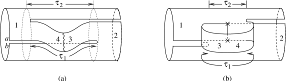
The resultant diagram (a) is nothing but the nonplanar diagram, generally slack $\mathchar 28956\relax_{1}\not=\mathchar 28956\relax_{2}$. For generic external states, both diagrams (a) and (b) contribute and their surface terms at $\mathchar 28956\relax_{2}=0$ are the same and cancel with each other. So generically the BRS invariance holds with these two diagrams alone. However, if the external states $\mathchar 28937\relax_{r}$ contain no $\mathchar 28939\relax_{n}^{-}$ modes, then the delta function factor $\mathchar 28942\relax(\mathchar 28956\relax_{1}-\mathchar 28956\relax_{2})$ appears and only the tight diagrams can contribute. This implies that the diagram (b) which contains backward propagation (i.e., $\mathchar 28956\relax_{1}=\mathchar 28939\relax_{4}T_{1}<0$) does not contribute from the start, and thus the counterterm which can cancel the surface term at $\mathchar 28956\relax_{1}=\mathchar 28956\relax_{2}=0$ of diagram (a) becomes missing. This is an anomaly of the BRS invariance in our SFT. As demonstrated in the present paper, the desired counterterm is supplied by the $UU$ diagram (b) in Fig. 2. We suspect that the BRS anomalies in our SFT occur this way only when the external states $\mathchar 28937\relax_{r}$ contain no $\mathchar 28939\relax_{n}^{-}$ modes. If so, then the relevant diagrams are always tight ones as in the light-cone gauge SFT and the anomalies for BRS and Lorentz invariance in both theories will come from the same type of diagrams.

A $\mathchar 28960\relax\,(\mathchar 28954\relax,w)$ and $\mathchar 28960\relax\,(z,q^{2})$

In the text, we have used the same variables as defined in GSW:[12]

$$\cases{\mathchar 28954\relax=e^{2\mathchar 28953\relax i{\tilde{\mathchar 28956\relax}}\mathchar 28951\relax}\cr w=e^{2\mathchar 28953\relax i{\tilde{\mathchar 28956\relax}}}\cr},\qquad\cases{z=e^{2\mathchar 28953\relax i\mathchar 28951\relax}\cr q^{2}=e^{2\mathchar 28953\relax i\mathchar 28956\relax}\cr},$$ (A.1)

with $\mathchar 28956\relax=-1/{\tilde{\mathchar 28956\relax}}$. Then, clearly, $(z,q^{2})$ corresponds to $(\mathchar 28951\relax,\mathchar 28956\relax)$ by the same relation as $(\mathchar 28954\relax,w)$ to $(\tilde{\mathchar 28951\relax}\equiv{\tilde{\mathchar 28956\relax}}\mathchar 28951\relax,{\tilde{\mathchar 28956\relax}})$. We have the following correspondences in the same manner:

$$\left\{\begin{array}[]{ccc}(\mathchar 28954\relax,w)&\leftrightarrow&({\tilde{\mathchar 28956\relax}}\mathchar 28951\relax,{\tilde{\mathchar 28956\relax}})\\ (z,q^{2})&\leftrightarrow&(\mathchar 28951\relax,\mathchar 28956\relax)\\ (qz,q^{2})&\leftrightarrow&(\mathchar 28951\relax+{\mathchar 28956\relax\over 2},\mathchar 28956\relax)\\ (z^{-1/2},q^{2})&\leftrightarrow&(-{\mathchar 28951\relax\over 2},\mathchar 28956\relax)\end{array}\right.$$ (A.2)

The functions $\mathchar 28960\relax,\ \mathchar 28960\relax^{T}$ and $\mathchar 28960\relax^{N}$ defined in the text are also the same as those in GSW, and are rewritten as follows in terms of the Jacobi theta functions:

$$\cases{\displaystyle\mathchar 28960\relax(\mathchar 28954\relax,w)=-2\mathchar 28953\relax ie^{\mathchar 28953\relax i({\tilde{\mathchar 28956\relax}}\mathchar 28951\relax)^{2}/{\tilde{\mathchar 28956\relax}}}{\mathchar 28963\relax_{1}\left({\tilde{\mathchar 28956\relax}}\mathchar 28951\relax|{\tilde{\mathchar 28956\relax}}\right)\over\mathchar 28963\relax^{\prime}_{1}\left(0|{\tilde{\mathchar 28956\relax}}\right)}={2\mathchar 28953\relax i\over\mathchar 28956\relax}{\mathchar 28963\relax_{1}\left(\mathchar 28951\relax|\mathchar 28956\relax\right)\over\mathchar 28963\relax^{\prime}_{1}\left(0|\mathchar 28956\relax\right)}\,,\cr\displaystyle\mathchar 28960\relax^{T}(\mathchar 28954\relax,w)=2\mathchar 28953\relax e^{\mathchar 28953\relax i({\tilde{\mathchar 28956\relax}}\mathchar 28951\relax)^{2}/{\tilde{\mathchar 28956\relax}}}{\mathchar 28963\relax_{2}\left({\tilde{\mathchar 28956\relax}}\mathchar 28951\relax|{\tilde{\mathchar 28956\relax}}\right)\over\mathchar 28963\relax^{\prime}_{1}\left(0|{\tilde{\mathchar 28956\relax}}\right)}={2\mathchar 28953\relax\over\mathchar 28956\relax}e^{\mathchar 28953\relax i(\mathchar 28951\relax+\mathchar 28956\relax/4)}{\mathchar 28963\relax_{1}\left(\mathchar 28951\relax+{\mathchar 28956\relax\over 2}|\mathchar 28956\relax\right)\over\mathchar 28963\relax^{\prime}_{1}\left(0|\mathchar 28956\relax\right)}\,,\cr\displaystyle\mathchar 28960\relax^{N}(\mathchar 28954\relax,w)=-2\mathchar 28953\relax ie^{\mathchar 28953\relax i({\tilde{\mathchar 28956\relax}}\mathchar 28951\relax)^{2}/{\tilde{\mathchar 28956\relax}}}{\mathchar 28963\relax_{1}\left({\tilde{\mathchar 28956\relax}}\mathchar 28951\relax|{\tilde{\mathchar 28956\relax}}+\frac{1}{2}\right)\over\mathchar 28963\relax^{\prime}_{1}\left(0|{\tilde{\mathchar 28956\relax}}+\frac{1}{2}\right)}=-{4\mathchar 28953\relax i\over\mathchar 28956\relax}{\mathchar 28963\relax_{1}\left(-{\mathchar 28951\relax\over 2}|{\mathchar 28956\relax\over 4}+\frac{1}{2}\right)\over\mathchar 28963\relax^{\prime}_{1}\left(0|{\mathchar 28956\relax\over 4}+\frac{1}{2}\right)}\,,\cr}$$ (A.3)

where the second equalities follow from the modular transformation properties of the theta functions. Now in view of the correspondences in Eq. (A.2), the comparison of the first and second expressions of $\mathchar 28960\relax(\mathchar 28954\relax,w)$ immediately leads to the relation

$$\mathchar 28960\relax(\mathchar 28954\relax,w)=-{1\over\mathchar 28956\relax}e^{-\mathchar 28953\relax i\mathchar 28951\relax^{2}/\mathchar 28956\relax}\mathchar 28960\relax(z,q^{2}).$$ (A.4)

Comparison of the second expression of $\mathchar 28960\relax^{T}(\mathchar 28954\relax,w)$ with the first one of $\mathchar 28960\relax(\mathchar 28954\relax,w)$ gives

$$\mathchar 28960\relax^{T}(\mathchar 28954\relax,w) = {i\over\mathchar 28956\relax}e^{\mathchar 28953\relax i(\mathchar 28951\relax+\mathchar 28956\relax/4)}e^{-\mathchar 28953\relax i(\mathchar 28951\relax+{\mathchar 28956\relax/2})^{2}/\mathchar 28956\relax}\mathchar 28960\relax(qz,q^{2})={i\over\mathchar 28956\relax}e^{-\mathchar 28953\relax i\mathchar 28951\relax^{2}/\mathchar 28956\relax}\mathchar 28960\relax(qz,q^{2}).\hskip 20.00003pt$$ (A.5)

Further, comparing the first and second expressions of $\mathchar 28960\relax^{N}(\mathchar 28954\relax,w)$, we obtain

$$\mathchar 28960\relax^{N}(\mathchar 28954\relax,w) = {2\over\mathchar 28956\relax}e^{-\mathchar 28953\relax i(-\mathchar 28951\relax/2)^{2}\over\mathchar 28956\relax/4}\mathchar 28960\relax^{N}(z^{-1/2},q^{1/2})={2\over\mathchar 28956\relax}e^{-\mathchar 28953\relax i\mathchar 28951\relax^{2}/\mathchar 28956\relax}\mathchar 28960\relax^{N}(z^{-1/2},q^{1/2}).\hskip 20.00003pt$$ (A.6)

Moreover, using $\mathchar 28963\relax_{1}(-\mathchar 28951\relax|\mathchar 28956\relax)=-\mathchar 28963\relax_{1}(\mathchar 28951\relax|\mathchar 28956\relax)$ and $e^{\mathchar 28953\relax i(\mathchar 28951\relax+\mathchar 28956\relax)^{2}/\mathchar 28956\relax}\mathchar 28963\relax_{1}(\mathchar 28951\relax+\mathchar 28956\relax|\mathchar 28956\relax)=-e^{\mathchar 28953\relax i\mathchar 28951\relax^{2}/\mathchar 28956\relax}\mathchar 28963\relax_{1}(\mathchar 28951\relax|\mathchar 28956\relax)$, we immediately find

$$\cases{\mathchar 28960\relax(z^{-1},q^{2})=-\mathchar 28960\relax(z,q^{2})\cr\mathchar 28960\relax(q^{2}z,q^{2})=-\mathchar 28960\relax(z,q^{2})\cr}.$$ (A.7)

Fig. 13: The contours $C_{1}$ and $C_{2}$ for $V_{\propto}$ case.

References

- [1] T. Kugo and T. Takahashi, Prog. Theor. Phys. 99 (1998), 649.
- [2] T. Asakawa, T. Kugo and T. Takahashi, Prog. Theor. Phys. 100 (1998), 831.
- [3] A. LeClair, M. E. Peskin and C. R. Preitschopf, Nucl. Phys. B317 (1989), 411.
- [4] L. Alvarez-Gaumé, C. Gomez, G. Moore and C. Vafa, Nucl. Phys. B303 (1988), 411.
- [5] S. B. Giddings and E. Martinec, Nucl. Phys. B278 (1986), 91.
- [6] T. Kugo and K. Suehiro, Nucl. Phys. B337 (1990), 434.
- [7] T. Kugo and B. Zwiebach, Prog. Theor. Phys. 87 (1992), 801.
- [8] A. LeClair, M. E. Peskin and C. R. Preitschopf, Nucl. Phys. B317 (1989), 464.
- [9] Y. Saitoh and Y. Tanii, Nucl. Phys. B325 (1989), 161.
- [10] Y. Saitoh and Y. Tanii, Nucl. Phys. B331 (1990), 744.
- [11] K. Kikkawa and S. Sawada, Nucl. Phys. B335 (1990), 677.
- [12] M. B. Green, J. H. Schwarz and E. Witten, Superstring Theory, (Cambridge Univ. Press, Cambridge, 1987).
- [13] T. Asakawa, T. Kugo and T. Takahashi, Prog. Theor. Phys. 100 (1998), 437.
- [14] M. Kaku and K. Kikkawa, Phys. Rev. D10 (1974), 1823.
- [15] S. Mandelstam, in Unified String Theories, ed. by M. Green and D. Gross (World Scientific, Singapore, 1986), p46.
- [16] D. Z. Freedman, S. B. Giddings, J. A. Shapiro and C. B. Thorn, Nucl. Phys. B298 (1988), 253.
- [17] E. T. Whittaker and G. N. Watson, A Course of Modern Aanlysis, (Cambridge Univ. Press, London, 1927), Chapters XX and XXI.
- [18] M. R. Dougras and B. Grinstein, Phys. Lett. 183B (1987), 52.
- [19] S. Weinberg, Phys. Lett. 187B (1987), 278.
- [20] H. Itoyama and P. Moxhay, Nucl. Phys. B293 (1987), 685.
- [21] N. Ohta, Phys. Rev. Lett. 59 (1987), 176.
- [22] M. Kaku and K. Kikkawa, Phys. Rev. D10 (1974), 1110.
- [23] E. D’Hoker and S. B. Giddings, Nucl. Phys. B291 (1987), 90.
- [24] H. Hata, K. Itoh, T. Kugo, H. Kunitomo and K. Ogawa, Phys. Rev. D34 (1986), 2360.