FTUAM-99-12; IFT-UAM/CSIC-99-16 INLO-PUB-8/99

Abstract: We give the analytic result for the fermion zero-mode of the $SU(2)$ calorons with non-trivial holonomy. It is shown that the zero-mode is supported on only one of the constituent monopoles. We discuss some of its implications.

1 Introduction

In this paper we give the exact expression for the $SU(2)$ fermion zero-mode in the field of the infinite volume caloron with non-trivial holonomy and unit charge. Study of the gauge field configurations had, somewhat surprisingly, revealed that at non-trivial holonomy calorons have two BPS monopoles ($N$ for $SU(N)$) as their constituents [1, 2, 3]. For the Harrington-Shepard [4] solution with trivial holonomy this is hidden, because one of the constituents is massless (it can be removed by a singular gauge transformation to show that the caloron for a large scale parameter becomes a single BPS monopole [5]). We find for calorons with well-separated constituents, that the fermion zero-mode is entirely supported on one of them. In itself it is not surprising that the zero-mode is correlated to the monopole constituents. Independently this observation was recently also made for gluino zero-modes in the context of supersymmetric gauge theories [6]. Gluinos are in the adjoint representation of the gauge group, such that there are four zero-modes, that can be split in pairs associated to each of the two constituents [6]. However, for the Dirac fermion there is only one zero-mode. To understand the “affinity” of the zero-mode to only one of the two monopoles, we will analyse in some detail what distinguishes them.

Calorons are characterised by the (fixed) holonomy [1, 7]. In the gauge in which $A_{\mu}(x)$ is periodic, this holonomy is given by

$${{\cal P}_{\infty}}=\lim_{|\vec{x}|\rightarrow\infty}{\rm P}\exp\left(\int_{0}^{\beta}A_{0}(t,\vec{x})dt\right)\equiv\exp(2\pi i\vec{\omega}\cdot\vec{\tau}).$$ (1)

Solutions are simplest in the so-called “algebraic” gauge, for which

$$A_{\mu}(t+\beta,\vec{x})={{\cal P}_{\infty}}A_{\mu}(t,\vec{x}){{\cal P}_{\infty}}^{-1},\quad\Psi^{\pm}_{z}(t+\beta,\vec{x})=\pm{{\cal P}_{\infty}}\Psi_{z}^{\pm}(t,\vec{x}).$$ (2)

We will generalise the problem of finding the fermion zero-mode in the field of the caloron with non-trivial holonomy, by adding a curvature free Abelian field, which forms the basis for the Nahm transformation [8]. Why this is useful will be evident from the construction. The equation to be solved is

$$\bar{D}_{z}\Psi_{z}(x)\equiv\bar{\sigma}_{\mu}(\partial_{\mu}+A_{\mu}(x)-2\pi iz_{\mu})\Psi_{z}(x)=0,$$ (3)

with $\bar{\sigma}_{\mu}=\sigma_{\mu}^{\dagger}=(1,-i\vec{\tau})$ and $\tau_{a}$ the Pauli matrices. For calorons, defined on $R^{3}\times S^{1}$, i.e. at finite temperature $1/\beta$, one can choose $z_{1}=z_{2}=z_{3}=0$ (the plane-wave factor $\exp(2\pi i\vec{z}\cdot\vec{x})$ does not affect the boundary conditions or the normalisation of the zero-mode and can be used to remove the $\vec{z}$ dependence). But $z=z_{0}$ will be arbitrary (it has a dual period of $1/\beta$). The zero-modes are represented as two-component spinors in the (chiral) Weyl decomposition for massless Dirac fermions.

2 ADHM construction

The construction of the zero-mode is best done in the ADHM formalism [9]. We will be brief in reviewing this formalism, further details can be found in ref. [1, 10, 11, 12]. In general the ADHM construction involves an operator $\Delta(x)$ (the “dual” of eq. (3)), whose normalised zero-mode, $\Delta^{\dagger}(x)v(x)=0$, gives the gauge field as $A_{\mu}(x)=v^{\dagger}(x)\partial_{\mu}v(x)$. For $SU(2)$ instantons of charge $k$ one has $\Delta^{\dagger}=(\lambda^{\dagger},B^{\dagger}-x^{\dagger})$, with $x^{\dagger}=x_{\mu}\bar{\sigma}_{\mu}$, $\lambda$ a $k$ dimensional row vector and $B$ a $k\times k$ symmetric matrix, all with values in the quaternions ($\lambda^{\ell}_{iI}$, $B^{\ell,m}_{IJ}=B^{m,\ell}_{IJ}$, with $\ell,m=1,\cdots,k$ “charge” and $I,J=1,2$ spinor indices, whereas $i=1,2$ is a colour index). Introducing the row vector $u^{\dagger}(x)\equiv\lambda(B-x)^{-1}$ and the scalar (real quaternion) $\phi(x)=1+u^{\dagger}(x)u(x)$, it can be shown [10, 11, 12] that the instanton gauge field and the $k$ zero-modes are given by

$$A_{\mu}(x)=\phi^{-1}(x){\rm Im}\left(u^{\dagger}(x)\partial_{\mu}u(x)\right),\quad\Psi^{\ell}_{iJ}(x)=\pi^{-1}\phi^{-{\scriptstyle{{1\over 2}}}}(x)(u^{\dagger}(x)f_{x})^{\ell}_{iI}\,\varepsilon_{IJ},$$ (4)

where $f_{x}$ is the matrix inverse, or Green’s function,

$$f_{x}=\left((B-x)^{\dagger}(B-x)+\lambda^{\dagger}\lambda\right)^{-1}.$$ (5)

Essential in the ADHM construction is that $\lambda$ and $B$ satisfy a quadratic constraint, which is equivalent to $f_{x}$ being a symmetric matrix whose imaginary quaternion components vanish, $(f_{x})^{\ell,m}_{IJ}\equiv f_{x}^{\ell,m}\delta_{IJ}$. From this alone it can be proven that the gauge field is self-dual and that the $\Psi^{\ell}(x)$ are zero-modes, $\bar{D}\Psi^{\ell}(x)\equiv\bar{\sigma}_{\mu}(\partial_{\mu}+A_{\mu}(x))\Psi^{\ell}(x)=0$. Its proper normalisation and the topological charge are read off from the remarkable results [10, 11, 12]

$$\Psi^{\ell}(x)^{\dagger}\Psi^{m}(x)=-(2\pi)^{-2}\partial_{\mu}^{2}f_{x}^{\ell,m},\quad{\rm Tr}F_{\mu\nu}^{\,2}(x)=-\partial_{\mu}^{2}\partial_{\nu}^{2}\log\det f_{x},$$ (6)

using $\lim_{|x|\rightarrow\infty}f_{x}^{\ell,m}=\delta^{\ell,m}|x|^{-2}$. Before addressing the explicit form of these expressions for the caloron with non-trivial holonomy, we perform one further simplification (for the details follow eqs. (21-29) in ref. [1], see also ref. [10]),

$$A_{\mu}(x)={\scriptstyle{{1\over 2}}}\phi(x)\partial_{\nu}\left(\lambda\bar{\eta}_{\mu\nu}f_{x}\lambda^{\dagger}\right),\quad\Psi^{\ell}_{iJ}(x)=(2\pi)^{-1}\phi^{\scriptstyle{{1\over 2}}}(x)\partial_{\mu}\left(\lambda f_{x}\bar{\sigma}_{\mu}\right)^{\ell}_{iI}\varepsilon_{IJ},$$ (7)

where the anti-selfdual ’t Hooft tensor $\bar{\eta}$ is defined by $\bar{\eta}^{i}_{0j}=-\bar{\eta}^{i}_{j0}=\delta_{ij}$ and $\bar{\eta}^{i}_{jk}=\varepsilon_{ijk}$ (furthermore $\varepsilon_{12}=1$ and with our conventions of $t=x_{0}$, $\varepsilon_{0123}=-1$).

The caloron with non-trivial holonomy is found by imposing boundary conditions to compactify time to a circle $u^{\ell+1}(t+\beta,\vec{x})=u^{\ell}(t,\vec{x}){\cal P}_{\infty}^{\dagger}$, which is easily seen to give the correct boundary conditions for the gauge field. For the general form of $\lambda$ and $B$ which respect this symmetry, see ref. [1]. Note that now the index $\ell$ runs over the set of all integers; the $R^{4}$ configuration with these boundary conditions has infinite topological charge (unit topological charge per time-period). To obtain the zero-mode with the appropriate boundary condition we note that with eq. (4)

$$\hat{\Psi}_{z}(x)\equiv\sum_{\ell}e^{-2\pi i\ell\beta z}\Psi^{\ell}(x),$$ (8)

satisfies the boundary condition $\hat{\Psi}_{z}(t+\beta,\vec{x})=e^{-2\pi i\beta z}{{\cal P}_{\infty}}\hat{\Psi}_{z}(t,\vec{x})$ and satisfies $\bar{D}\hat{\Psi}_{z}(x)=0$ for all $z$. The general solution of the Weyl equation, eq. (3), with both periodic and anti-periodic boundary conditions is now easily found (for simplicity we put $\beta=1$)

$$\Psi^{+}_{z}(x)=e^{2\pi izt}\hat{\Psi}_{z}(x),\quad\Psi^{-}_{z}(x)=e^{2\pi izt}\hat{\Psi}_{z+1/2}(x).\quad$$ (9)

In particular $\Psi^{-}(x)=\Psi^{-}_{0}(x)=\hat{\Psi}_{1/2}(x)$ is the, for finite temperature, physically relevant chiral zero-mode in the background of a caloron, whereas $\Psi^{+}(x)=\Psi^{+}_{0}(x)=\hat{\Psi}_{0}(x)$ is relevant for compactifications.

3 Nahm-Fourier transformation

The interpretation of the “charge” index as a Fourier index, as suggested by the construction of the caloron zero-mode, has been essential for solving the quadratic ADHM constraint in the presence of non-trivial holonomy. It maps the ADHM construction to the Nahm formalism, in which furthermore $f_{x}$ is solved in terms of a quantum mechanics problem on the circle ($z\in[0,1]$) with a piecewise constant potential and delta function singularities determined by the holonomy [1]. The relevant quantities involved are

$$\hat{f}_{x}(z,z^{\prime})=\sum_{\ell,m}f_{x}^{\ell,m}e^{2\pi i(\ell z-mz^{\prime})},\quad\hat{\lambda}(z)=\sum_{\ell}\lambda^{\ell}e^{-2\pi i\ell z},$$ (10)

where matrix multiplication is replaced by convolution in the usual sense. The solution of the ADHM constraint implies that $\hat{\lambda}(z)$ is the sum of two delta functions. Together with the explicit expression for the Green’s function $\hat{f}_{x}(z,z^{\prime})$ as given in eqs. (47-49) of ref. [1], the zero-mode reads

$$\hat{\Psi}_{z}(x)=(2\pi)^{-1}\phi^{\scriptstyle{{1\over 2}}}(x)\partial_{\mu}\left(\int_{0}^{1}dz^{\prime}\hat{\lambda}(z^{\prime})\hat{f}_{x}(z^{\prime},z)\bar{\sigma}_{\mu}\right)_{iI}\varepsilon_{IJ},$$ (11)

cmp. eq. (4). Whereas eq. (6) yields

$$\hat{\Psi}_{z^{\prime}}^{\dagger}(x)\hat{\Psi}_{z}(x)=-(2\pi)^{-2}\partial_{\mu}^{2}\hat{f}_{x}(z^{\prime},z).$$ (12)

4 Explicit expressions

Using the classical scale invariance to put $\beta=1$, one has [1]

$$s(x)=-{\scriptstyle{{1\over 2}}}{\rm Tr}F_{\mu\nu}^{\,2}(x)=-{\scriptstyle{{1\over 2}}}\partial_{\mu}^{2}\partial_{\nu}^{2}\log\psi(x),\quad\psi(x)=\hat{\psi}(\vec{x})-\cos(2\pi t),\quad\hat{\psi}(\vec{x})={\scriptstyle{{1\over 2}}}{\rm tr}({\cal A}_{2}{\cal A}_{1}),$$ (13)

where

$${\cal A}_{m}\equiv\frac{1}{r_{m}}\left(\!\!\!\begin{array}[]{cc}r_{m}\!\!&|\vec{y}_{m}\!\!-\!\vec{y}_{m+1}|\\ 0\!\!&r_{m+1}\end{array}\!\!\!\right)\left(\!\!\!\begin{array}[]{cc}c_{m}\!\!&s_{m}\\ s_{m}\!\!&c_{m}\end{array}\!\!\!\right).$$ (14)

Noting that $r_{3}\equiv r_{1}$ and $\vec{y}_{3}\equiv\vec{y}_{1}$ we defined $r_{m}=|\vec{x}-\vec{y}_{m}|$, with $\vec{y}_{m}$ the position of the $m^{\rm th}$ constituent monopole, which can be assigned a mass $8\pi^{2}\nu_{m}$, where $\nu_{1}=2\omega$ and $\nu_{2}=2\bar{\omega}\equiv 1-2\omega$. Furthermore, $c_{m}\equiv\cosh(2\pi\nu_{m}r_{m})$, $s_{m}\equiv\sinh(2\pi\nu_{m}r_{m})$ and $\pi\rho^{2}=|\vec{y}_{2}-\vec{y}_{1}|$.

New is the result for the zero-mode density

$$|\Psi^{-}(x)|^{2}=-(2\pi)^{-2}\partial_{\mu}^{2}\hat{f}_{x}({\scriptstyle{{1\over 2}}},{\scriptstyle{{1\over 2}}}),\quad|\Psi^{+}(x)|^{2}=-(2\pi)^{-2}\partial_{\mu}^{2}\hat{f}_{x}(0,0),$$ (15)

defined by [1]

$$\hat{f}_{x}({\scriptstyle{{1\over 2}}},{\scriptstyle{{1\over 2}}})=\frac{\pi}{r_{1}r_{2}\psi(x)}\left\{s_{2}[r_{1}c_{1}+\pi\rho^{2}s_{1}]+r_{2}s_{1}+\frac{c_{2}\!-\!1}{r_{2}}[\pi\rho^{2}r_{1}c_{1}+{\scriptstyle{{1\over 2}}}(r_{1}^{2}+r_{2}^{2}+\pi^{2}\rho^{4})s_{1}]\right\},$$

$$\hat{f}_{x}(0,0)=\frac{\pi}{r_{1}r_{2}\psi(x)}\left\{s_{1}[r_{2}c_{2}+\pi\rho^{2}s_{2}]+r_{1}s_{2}+\frac{c_{1}\!-\!1}{r_{1}}[\pi\rho^{2}r_{2}c_{2}+{\scriptstyle{{1\over 2}}}(r_{1}^{2}+r_{2}^{2}+\pi^{2}\rho^{4})s_{2}]\right\}.$$ (16)

By a suitable combination of a constant gauge transformation, spatial rotation and translation we can arrange both $\vec{\omega}=(0,0,\omega)$ and the constituents at $\vec{y}_{1}=(0,0,\nu_{2}\pi\rho^{2})$ and $\vec{y}_{2}=(0,0,-\nu_{1}\pi\rho^{2})$. For this choice we find

$$A_{\mu}(x)=\frac{i}{2}\bar{\eta}^{3}_{\mu\nu}\tau_{3}\partial_{\nu}\log\phi(x)+\frac{i}{2}\phi(x){\rm Re}\left((\bar{\eta}^{1}_{\mu\nu}-i\bar{\eta}^{2}_{\mu\nu})(\tau_{1}+i\tau_{2})\partial_{\nu}\chi(x)\right),$$ (17)

$$\Psi^{-}_{1I}(x)=(2\pi)^{-1}\rho\phi^{\scriptstyle{{1\over 2}}}(x)\pmatrix{\partial_{2}+i\partial_{1}\cr\partial_{0}-i\partial_{3}\cr}\hat{f}_{x}(\omega,{\scriptstyle{{1\over 2}}}),\quad\Psi^{-}_{2I}(x)=\Psi^{-}_{1J}(x)^{*}\varepsilon_{JI},$$

$$\Psi^{+}_{1I}(x)=(2\pi)^{-1}\rho\phi^{\scriptstyle{{1\over 2}}}(x)\pmatrix{\partial_{2}+i\partial_{1}\cr\partial_{0}-i\partial_{3}\cr}\hat{f}_{x}(\omega,0),\quad\Psi^{+}_{2I}(x)=\Psi^{+}_{1J}(x)^{*}\varepsilon_{JI},$$ (18)

with $\phi^{-1}(x)=1-\frac{\pi\rho^{2}}{\psi(x)}\left(\frac{s_{1}c_{2}}{r_{1}}+\frac{s_{2}c_{1}}{r_{2}}+\frac{\pi\rho^{2}s_{1}s_{2}}{r_{1}r_{2}}\right)$ and $\chi(x)=\frac{\pi\rho^{2}}{\psi(x)}\left(e^{-2\pi it}\frac{s_{1}}{r_{1}}+\frac{s_{2}}{r_{2}}\right)e^{2\pi i\nu_{1}t}$, and

$$\hat{f}_{x}(\omega,{\scriptstyle{{1\over 2}}})=\frac{\pi e^{\pi i\nu_{1}t}}{r_{1}r_{2}\psi(x)}\left\{\left(e^{\pi it}r_{1}\!+\!e^{-\pi it}[\pi\rho^{2}s_{1}\!+\!r_{1}c_{1}]\right)\sinh(\pi r_{2}\nu_{2})\!+\!e^{-\pi it}r_{2}s_{1}\cosh(\pi r_{2}\nu_{2})\right\},$$

$$\hat{f}_{x}(\omega,0)=\frac{\pi e^{-\pi i\nu_{2}t}}{r_{1}r_{2}\psi(x)}\left\{\left(e^{-\pi it}r_{2}+e^{\pi it}[\pi\rho^{2}s_{2}\!+\!r_{2}c_{2}]\right)\sinh(\pi r_{1}\nu_{1})+e^{\pi it}r_{1}s_{2}\cosh(\pi r_{1}\nu_{1})\right\}.$$ (19)

5 Properties of the zero-mode

The gauge field has a symmetry under the anti-periodic gauge transformation $g(x)=\exp(\pi it\hat{\omega}\cdot\vec{\tau})$, which changes the sign of the holonomy, ${{\cal P}_{\infty}}\rightarrow-{{\cal P}_{\infty}}$, or $\omega\leftrightarrow\bar{\omega}={\scriptstyle{{1\over 2}}}-\omega$. An anti-periodic gauge transformation does, however, not leave fermions invariant, and indeed it interchanges $\Psi^{+}_{z}(x)$ and $\Psi^{-}_{z}(x)$. To preserve the special choice of parametrisation presented above, the change of sign in the holonomy, which interchanges $\nu_{1}$ and $\nu_{2}$, is also accompanied by an interchange of the constituent locations. This indeed leaves the action density invariant. That the zero-mode clearly distinguishes between the two cases becomes evident in the static limit, $\rho\rightarrow\infty$ (or equivalently $\beta\rightarrow 0$), in which case the zero-mode is completely localised on one of the constituent monopoles, as follows from (cmp. eq. (16))

$$\lim_{\rho\rightarrow\infty}|\Psi^{-}(x)|^{2}=-\partial_{\mu}^{2}\left\{\frac{\tanh(\pi r_{2}\nu_{2})}{4\pi r_{2}}\right\},\quad\lim_{\rho\rightarrow\infty}|\Psi^{+}(x)|^{2}=-\partial_{\mu}^{2}\left\{\frac{\tanh(\pi r_{1}\nu_{1})}{4\pi r_{1}}\right\}.$$ (20)

Under the anti-periodic gauge transformation the anti-periodic zero-mode becomes periodic. The new anti-periodic zero-mode is now completely localised on the other constituent monopole (this is consistent with the fact that $\hat{f}_{x}(0,0)$ can be obtained from $\hat{f}_{x}({\scriptstyle{{1\over 2}}},{\scriptstyle{{1\over 2}}})$ by interchanging $r_{1}$ and $\nu_{1}$ with $r_{2}$ and $\nu_{2}$). Figure 1 illustrates these issues [13].

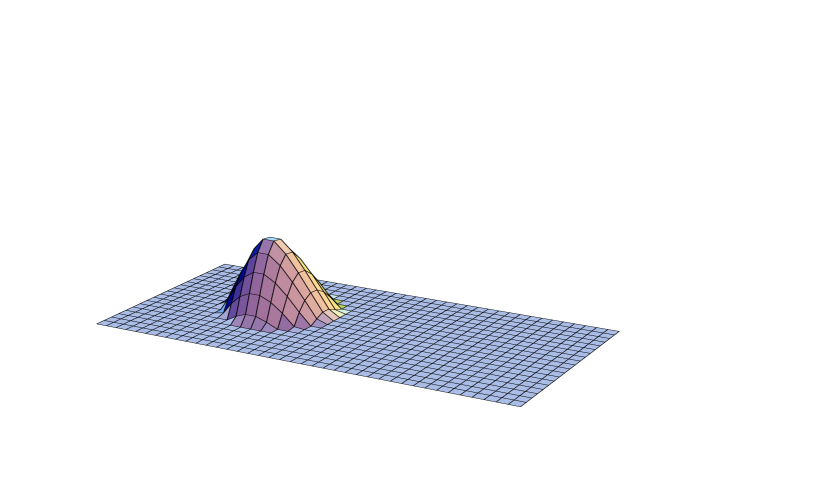
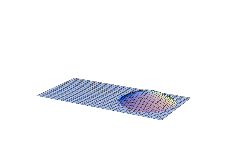
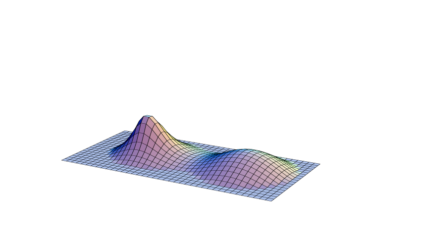
Figure 1: For the two figures on the sides we plot on the same scale the logarithm of the zero-mode densities (cutoff below $1/e^{5}$) for $\omega=1/8$ (left $\Psi^{-}$ / right $\Psi^{+}$) and $\omega=3/8$ (right $\Psi^{-}$ / left $\Psi^{+}$), with $\beta=1$ and $\rho=1.2$. In the middle figure we show for the same parameters (both choices of $\omega$ give the same action density) the logarithm of the action density (cutoff below $1/2e^{2}$).

In the gauge where $A_{\mu}(x)$ is periodic, for large $\rho$ one of the constituent monopole fields is completely time independent, whereas the other one has a time dependence that would result from a full rotation along the axis connecting the two constituents [1]. This is read off from

$$\hskip-17.07164ptA_{\mu}^{\rm per}=\frac{i}{2}\bar{\eta}^{3}_{\mu\nu}\tau_{3}\partial_{\nu}\log\phi+\frac{i}{2}\phi{\rm Re}\left((\bar{\eta}^{1}_{\mu\nu}-i\bar{\eta}^{2}_{\mu\nu})(\tau_{1}+i\tau_{2})(\partial_{\nu}+4\pi i\omega\delta_{\nu,0})\tilde{\chi}\right)\!+\!\delta_{\mu,0}2\pi i\omega\tau_{3},$$ (21)

$$\hskip-17.07164pt\tilde{\chi}=e^{-4\pi it\omega}\chi=\frac{4\pi\rho^{2}}{(r_{2}+r_{1}+\pi\rho^{2})^{2}}\left\{r_{2}e^{-2\pi r_{2}\nu_{2}}e^{-2\pi it}\!+r_{1}e^{-2\pi r_{1}\nu_{1}}\right\}\left(1\!+\!{\cal O}(e^{-4\pi\,{\rm min}(r_{1}\nu_{1},r_{2}\nu_{2})})\right).$$

(Note that for large $\rho$, $\phi(x)$ becomes time independent.) This full rotation - which we will call the Taubes-winding - is responsible for the topological charge of the otherwise time independent monopole pair [14]. Under the anti-periodic gauge transformation that changes the sign of the holonomy the Taubes-winding is supported by the other constituent. It has not gone unnoticed that the anti-periodic fermion zero-mode is precisely localised on the monopole constituent that carries the Taubes-winding. Another way to distinguish the two constituent monopoles is by inspecting the Polyakov loop values at their centers. One finds -1 for the monopole line with the Taubes-winding and +1 for the other monopole line (this is correlated to the vanishing of the would-be Higgs field), see the appendix of ref. [15]. For trivial holonomy, $\omega=0$, the Polyakov loop is indeed -1 at the center of the Harrington-Shepard [4] caloron. Its zero-mode, constructed before in ref. [7, 16], agrees with the results found here.

The association of the zero-mode with the constituent that carries the Taubes-winding lends considerable support for the role of the monopole loops with Taubes-winding in QCD for chiral dynamics [1]. The precise embedding of these straight finite temperature monopole loops as curved monopole loops in flat space remains a non-trivial and challenging problem. Although it may seem contradictory to expect the zero-mode with anti-periodic boundary conditions to be the relevant one, one should not forget that for a curved monopole loop the spin frame makes also one full rotation due to the bending of the loop, thereby most likely providing the compensating sign flip.

References

• [1] T.C. Kraan and P. van Baal, Nucl. Phys. B533 (1998) 627 (hep-th/9805168).
• [2] T.C. Kraan and P. van Baal, Phys. Lett. B428 (1998) 268 (hep-th/9802049); Phys. Lett. B435 (1998) 389 (hep-th/9806034).
• [3] K. Lee and P. Yi, Phys. Rev. D56 (1997) 3711; K. Lee, Phys. Lett. B426 (1998) 323; K. Lee and C. Lu, Phys. Rev. D58 (1998) 025011.
• [4] B.J. Harrington and H.K. Shepard, Phys. Rev. D17 (1978) 2122; D18 (1978) 2990.
• [5] P. Rossi, Nucl. Phys. B149 (1979) 170.
• [6] T.J. Hollowood, V.V. Khoze, W. Lee and M.P. Mattis, Breakdown of cluster decomposition in instanton calculations of the gluino condensate, hep-th/9904116; N.M. Davies, T.J. Hollowood, V.V. Khoze and M.P. Mattis, Gluino condensate from magnetic monopoles in SUSY gluodynamics, to appear.
• [7] D.J. Gross, R.D. Pisarski and L.G. Yaffe, Rev. Mod. Phys. 53 (1983) 43.
• [8] W. Nahm, Phys. Lett. 90B (1980) 413; Self-dual monopoles and calorons, in: Lect. Notes in Physics. 201, eds. G. Denardo, e.a. (1984) p. 189.
• [9] M.F. Atiyah, N.J. Hitchin, V.G. Drinfeld, Yu. I. Manin, Phys. Lett. 65 A (1978) 185.
• [10] E.F. Corrigan, D.B. Fairlie, S. Templeton, P. Goddard, Nucl. Phys. B140 (1978) 31.
• [11] H. Osborn, Nucl. Phys. B140 (1978) 45; Ann. Phys. (N.Y.) 135 (1981) 373.
• [12] E. Corrigan and P. Goddard, Ann. Phys. (N.Y.) 154 (1984) 253.
• [13] C-programmes for action/zero-mode densities and Polyakov loops can be found at http://www-lorentz.leidenuniv.nl/vanbaal/Caloron.html.
• [14] C. Taubes, Morse theory and monopoles: topology in long range forces, in: Progress in gauge field theory, eds. G. ’t Hooft et al, (Plenum Press, New York, 1984) p. 563.
• [15] M. GarcΓ­a PΓ©rez, A. GonzΓ‘lez-Arroyo, A. Montero and P. van Baal, Calorons on the lattice – a new perspective, hep-lat/9903022.
• [16] N. Bilic, Phys. Lett. 97B (1980) 107; A. GonzΓ‘lez-Arroyo and Yu.A. Simonov, Nucl. Phys. B460 (1996) 429.