Towards exact results of QED from supersymmetry

Abstract

To obtain some exact results of U(1) gauge theory (QED), we construct the low energy effective action of N=2 supersymmetric QED with a massless matter and Fayet-Iliopoulos term, assuming no confinement. The harmonic superspace formalism for N=2 extended supersymmetry makes the construction easy. We analyze the vacuum structure and find no vacuum. It suggests the confinement in non-supersymmetric QED at low energies.

I Introduction

QED is the most successful quantum field theory in the phenomenological point of view. In fact, QED perfectly describes the electromagnetic interaction at low energies. However, there is a question whether QED is a fully consistent theory beyond the perturbation theory. QED has the Landau ghost problem[1] and the renormalized coupling constant vanishes. This means QED may be trivial as a quantum field theory, and it can only be regarded as a low energy effective theory.

On the other hand, Miransky suggested that QED is non-trivial[2]. He investigated a truncated Schwinger-Dyson equation for the fermion propagator and found a continuous chiral phase transition. He claimed that the chiral symmetry is spontaneously broken in the strong coupling phase. After his work, non-perturbative studies of QED have been done extensively[3, 4, 5]. Some of numerical simulations were carried out to understand whether QED is trivial or not. Kogut et al. claimed that the existence of a chiral phase transition was confirmed by numerical studies[6]. On the other hand, DESY-Jülich group claimed that QED is a trivial theory which is described by a Gaussian fixed point, and the critical behavior around it is similar to the one of the $\lambda\phi^{4}$ model[7]. This controversy is not resolved yet.

Recently, there has been much progress in the understanding of the non-perturbative dynamics of N=1 and N=2 supersymmetric four-dimension field theories. The exact superpotential can be derived in N=1 supersymmetric QCD (SQCD: supersymmetric SU$(N_{c})$ gauge theory with vector-like matters) [8], and the models with various gauge symmetries and matter contents have been investigated. Seiberg and Witten derived the exact low energy effective action for N=2 supersymmetric SU(2) Yang-Mills theory in Coulomb phase up to two derivatives[9], and generalized it to the case of N=2 SQCD [10]. Their method was applied to the different gauge groups and the solution was obtained.

Since we can derive the exact low energy effective action (LEEA) of N=2 supersymmetric gauge theories, we can expect to extract the exact information of non-supersymmetric gauge theories, QED and QCD, for example. A simple way to break supersymmetry is to add soft supersymmetry breaking terms. In Refs. [11, 12, 13, 14, 15, 16] soft breaking terms are used to explore N=1 supersymmetric QCD and the phase structure of these theories in the absence of supersymmetry. We will focus on N=2 supersymmetric QED (SQED) with a massless matter to explore N=0 QED. It is well known that Fayet-Iliopoulos (FI) term spontaneously breaks supersymmetry in N=2 SQED [17, 18, 19]. We construct the exact LEEA of SQED with FI term not introducing the soft breaking terms by hand.

In Refs. [9, 10][11, 12, 13, 14, 15, 16] N=1 superfields were used to describe N=2 supersymmetric theories. Therefore, N=2 supersymmetry was not manifest in those works. We can use constrained superfields on the standard N=2 superspace [20], but these are not appropriate to the construction and the analysis of the LEEA, because the description becomes extremely complicated when the interaction is included on. An elegant off-shell formulation of N=2 supersymmetry is the harmonic superspace formalism, developed by Galperin et al. [23]. In this formalism superfileds are unconstrained and we do not need to solve complicated constraints. N=2 supersymmetry is manifest at each step of the calculation. We will see that this formalism is very powerful for constructing the LEEA in this paper.

The plan of this paper is as follows. In Sec.II we briefly review the harmonic superspace formalism stressing some important points for our main. In Sec.III we construct the LEEA of SQED without the FI term as the first step. In Sec.IV we extend the discussion in the previous section to the case with FI term. In Sec.V we analyze the effective potential of the LEEA which is obtained in the previous section, and discuss the vacuum structure of N=0 QED. Sec.VI is devoted to the conclusion. Our notations and conventions are summarized in Appendix.

II Harmonic Superspace Formalism

We briefly review some of the basics of the harmonic superspace formalism (HSS). HSS is the formalism for N=2 extended supersymmetry developed by Galperin et al. [23]. The standard N=2 superspace is parameterized by the coordinates

$$\{x^{\mu},\theta_{\alpha i},{\bar{\theta}}_{\dot{\alpha}}^{i}\},$$ (1)

where $\alpha$ is the spinor index and $i$ is SU(2$)_{{\rm R}}$ index. The key ingredient in HSS is the harmonic variables $u_{i}^{\pm}$ which parameterize the coset space SU(2$)_{{\rm R}}$/U(1). The variables satisfy the relation

$$u^{+i}u_{i}^{-}=1,$$ (2)

where $\pm$ denote U(1) charge $\pm 1$. The variables of the harmonic superspace in the central basis (CB) are

$${\bf CB}:\{{x^{\mu},\theta_{\alpha i},{\bar{\theta}}_{\dot{\alpha}}^{i},u_{i}^{\pm}}\}.$$ (3)

Harmonic superfields are the functions of these variables. In CB the differentiation by the harmonic variables are defined as

$$D^{++}=u^{+i}\displaystyle\frac{\partial}{\partial u^{-i}},\hskip 5.69054ptD^{--}=u^{-i}\displaystyle\frac{\partial}{\partial u^{+i}},$$ (4)

and the integration over $u$ is defined by the following rules:

$$\displaystyle\int du\hskip 2.84526pt1=1,$$ (5)

$$\displaystyle\int du\hskip 2.84526ptu_{(i_{1}}^{+}\cdots u_{i_{n}}^{+}u_{j_{1}}^{-}\cdots u_{j_{m})}^{-}=0,\hskip 8.53581ptn+m>0,$$ (6)

where the parenthesis mean symmetrization of SU(2$)_{{\rm R}}$ indices. Namely, the $u$ integration is defined to pick up the SU(2$)_{{\rm R}}$ singlet part. The Lagrangian which is described by the harmonic superfields is not manifestly real under the usual complex conjugation. However, it is real under the conjugation which is the combination of the usual complex conjugation and the star conjugation. The star conjugation for the harmonic variables are defined by

$$(u_{i}^{+})^{*}=u_{i}^{-},\hskip 5.69054pt(u_{i}^{-})^{*}=-u_{i}^{+},$$ (7)

and other quantities are singlet under the conjugation. The harmonic variables are transformed under the combined conjugation as

$$\displaystyle{\overline{u^{\pm i}}}^{*}=-u_{i}^{\pm},\hskip 5.69054pt{\overline{u_{i}^{\pm}}}^{*}=u^{\pm i}.$$ (8)

There is another important basis called the analytic basis (AB):

$${\bf AB} : \{x^{\mu}_{A},\theta_{\alpha}^{\pm},{\bar{\theta}}_{\dot{\alpha}}^{\pm},u_{i}^{\pm}\},$$ (11)

$$x^{\mu}_{A}=x^{\mu}-2i\theta^{(i}\sigma^{\mu}{\bar{\theta}^{j)}}u_{i}^{+}u_{j}^{-},$$

$$\theta^{\pm}=\theta^{i}u_{i}^{\pm},\hskip 8.53581pt{\bar{\theta}}^{\pm}={\bar{\theta}}^{i}u_{i}^{\pm}.$$

Irreducible harmonic superfields are not the function of the entire variables of AB or CB but the function on their subspaces, the analytic subspace (ASS) or the chiral subspace (CSS). ASS is defined by

$${\bf ASS}:\zeta_{A} = \{x^{\mu}_{A},\theta^{+}_{\alpha},{\bar{\theta}}^{+}_{\dot{\alpha}},u^{\pm}_{i}\},$$ (12)

and it is an invariant subspace under N=2 supersymmetry transformation. This fact allows one to define the analytic superfields which satisfy the analyticity conditions

$$D^{+}\phi^{(q)}(\zeta_{A})={\bar{D}}^{+}\phi^{(q)}(\zeta_{A})=0,$$ (13)

where

$$D^{+}=D^{i}u_{i}^{+}=\displaystyle\frac{\partial}{\partial\theta^{-}},\hskip 5.69054pt{\bar{D}}^{+}={\bar{D}}^{i}u_{i}^{+}=\frac{\partial}{\partial{\bar{\theta}}^{-}},$$ (14)

and $q$ denotes U(1) charge of the field.

There are two basic supermultiplets in the N=2 supersymmetry: the hypermultiplet and the vectormultiplet. Fayet-Sohnius(FS) superfield [21] describes the complex hypermultiplet whose on-shell physical components are $(f^{i},\psi,\varphi)$, where $f^{i}$ is a complex scalar in SU(2$)_{{\rm R}}$ doublet, and $(\psi$, $\varphi)$ is a Dirac spinor. The superfield with U(1) charge $+1$ is written down as

$$\phi^{+}(\zeta_{A}) = F^{+}(x_{A},u^{\pm})+\sqrt{2}\theta^{+}\psi(x_{A},u^{\pm})+\sqrt{2}{{\bar{\theta}}^{+}}{\bar{\varphi}}(x_{A},u^{\pm})$$ (15)

$$+ \theta^{+}\theta^{+}M^{-}(x_{A},u^{\pm})+{\bar{\theta}}^{+}{\bar{\theta}}^{+}N^{-}(x_{A},u^{\pm})$$ (16)

$$+ \theta^{+}\sigma^{\mu}{\bar{\theta}}^{+}V_{\mu}(x_{A},u^{\pm})+\sqrt{2}{\bar{\theta}}^{+}{\bar{\theta}}^{+}\theta^{+}\xi_{\alpha}^{--}(x_{A},u^{\pm})$$ (17)

$$+ \sqrt{2}{\bar{\theta}}^{+}{\bar{\chi}}^{--}(x_{A},u^{\pm})+\theta^{+}\theta^{+}{\bar{\theta}}^{+}{\bar{\theta}}^{+}D^{---}(x_{A},u^{\pm}),$$ (18)

where $F^{+},M^{-},N^{-}$ and $D^{---}$ are complex scalar fields, $\psi,{\bar{\varphi}},\xi^{--}$ and ${\bar{\chi}}^{--}$ are Weyl fermion fields and $V_{\mu}$ is a complex vector field. Each component field can be expanded in $u^{\pm}_{i}$. For example,

$$F^{+}(x_{A},u^{\pm})=\displaystyle\sum_{n=0}^{\infty}f^{(i_{1}\cdots i_{n+1}j_{1}\cdots j_{n})}(x_{A})u^{+}_{(i_{1}}\cdots u^{+}_{i_{n+1}}u^{-}_{j_{1}}\cdots u^{-}_{j_{n})}.$$ (19)

Therefore, FS superfield includes infinite number of auxiliary fields. The action for a free complex FS hypermultiplet is given by

$$S_{{\rm FS}}=\displaystyle\int d\zeta_{A}^{(-4)}du\hskip 2.84526pt{\overline{\phi^{+}}}^{*}D^{++}\phi^{+},$$ (20)

where $D^{++}$ is a covariant derivative in AB given by Eq. (A29) and $d\zeta_{A}^{(-4)}$ is the analytic measure defined by

$$d\zeta_{A}^{(-4)}=d^{4}x_{A}d^{2}\theta^{+}d^{2}{\bar{\theta}}^{+}.$$ (21)

Solving the equation of motion $D^{++}\phi^{+}=0$, we can easily check that only the physical components $(f^{i},\psi,\varphi)$ remain and follow free equation of motions.

The on-shell physical components of a vectormultiplet are $(A,A_{\mu},\lambda^{i})$, where $A$ is a complex scalar, $A_{\mu}$ is a vector field and $\lambda^{i}$ is a Majorana spinor in SU(2$)_{{\rm R}}$ doublet. A vectormultiplet is described by the dimensionless analytic superfield $V^{++}$ of U(1) charge +2. It transforms under gauge transformation as

$$\delta V^{++}=-D^{++}\lambda(x_{A},u^{\pm})$$ (22)

in abelian case, where $\lambda$ is an analytic superfield with U(1) charge $0$. Here $V^{++}$ is chosen to be real, namely,

$$V^{++}={\overline{V^{++}}}^{*}.$$ (23)

If we take the Wess-Zumino-like gauge,

$$V^{++}(\zeta_{A}) = \theta^{+}\theta^{+}\frac{1}{\sqrt{2}}A(x_{A},u^{\pm})+{\bar{\theta}}^{+}{\bar{\theta}}^{+}\frac{1}{\sqrt{2}}A^{*}(x_{A},u^{\pm})+i\theta^{+}\sigma^{\mu}{\bar{\theta}}^{+}A_{\mu}(x_{A},u^{\pm})$$ (25)

$$+{\bar{\theta}}^{+}{\bar{\theta}}^{+}\theta^{+}2\lambda^{-}(x_{A},u^{\pm})+\theta^{+}\theta^{+}{\bar{\theta}}^{+}2{\bar{\lambda}}^{-}(x_{A},u^{\pm})+\theta^{+}\theta^{+}{\bar{\theta}}^{+}{\bar{\theta}}^{+}D^{--}(x_{A},u^{\pm}),$$

where $D^{--}=D^{(ij)}u_{i}^{-}u_{j}^{-}$ is a real auxiliary field in SU(2$)_{{\rm R}}$ triplet.

CSS is defined by

$${\bf CSS}:\zeta_{R} = \{x^{\mu}_{R},\theta_{\alpha i},u_{i}^{\pm}\},$$ (27)

$$x^{\mu}_{R}=x^{\mu}-i\theta^{i}\sigma^{\mu}{\bar{\theta}}_{i},$$

and the gauge field strength superfield $W$ is described as a function on it.

$$W(x_{R},\theta) = -\displaystyle\frac{1}{4}\int du({\bar{D}}^{+})^{2}V^{++}$$ (28)

$$= \displaystyle\frac{1}{\sqrt{2}}A^{*}(x_{R})-\frac{1}{3\sqrt{2}}\epsilon_{ik}\epsilon_{jl}(\theta^{i}\theta^{j})(\theta^{k}\theta^{l})\Box A(x_{R})-\frac{1}{4}\theta^{i}\sigma^{\mu}{\bar{\sigma}}^{\nu}\theta_{i}F_{\mu\nu}(x_{R})$$ (30)

$$+\theta^{i}\lambda_{i}(x_{R})+\frac{2}{3}i(\theta^{i}\theta^{j})(\theta^{k}\sigma^{\mu}\partial_{\mu}{\bar{\lambda}}^{l}(x_{R}))\epsilon_{ik}\epsilon_{jk}+\frac{1}{3}\epsilon_{ik}\epsilon_{jk}(\theta^{i}\theta^{j})D^{(kl)}(x_{R}).$$

The superfield which is a function on CSS is called the chiral superfield. Note that the chiral superfield $W$ does not explicitly depend on ${\bar{\theta}}_{i}$ and $u_{i}^{\pm}$ and can not the function on ASS. Also note that the analytic superfield can not be described as a function on CSS. The action of a vectormultiplet is given by

$$S_{{\rm gauge}}=\frac{1}{4\pi}{\rm Im}\tau\int d\zeta_{R}W^{2},$$ (31)

where $\tau=i\frac{4\pi}{e^{2}}+\frac{\Theta}{2\pi}$ with that $e$ is the gauge coupling and $\Theta$ is the vacuum angle. $d\zeta_{R}=d^{4}x_{R}d^{4}\theta du$ is the chiral subspace measure.

We write down the tree-level action of SQED with single matter as

$$S=\displaystyle\int d\zeta_{A}^{(-4)}du\hskip 2.84526pt{{\overline{\phi^{+}}}}^{*}(D^{++}+2iV^{++})\phi^{+}+\frac{1}{4\pi}{\rm Im}\tau\int d\zeta_{R}W^{2}.$$ (32)

The integrand of the first term (the analytic part) must have U(1) charge $+4$ and does not explicitly depend on $\theta^{-}$ and ${\bar{\theta}}^{-}$, i.e., it must be analytic. The chiral superfield does not appear in the analytic part, because the chiral superfield does not satisfy the analyticity. Similarly, we find that the analytic superfield does not appear in the integrand of the second term (the chiral part). The chiral part does not explicitly depend on ${\bar{\theta}_{i}}$ and $u_{i}^{\pm}$. These facts are important for constructing the LEEA.

III Construction of the LEEA without Fayet-Iliopoulos term

In this section we construct the LEEA of SQED with single massless matter using the harmonic superspace formalism. In the next section we apply the method used in this section to the case of including FI term. The tree-level action leads the scalar potential

$$V=|\sqrt{2}A|^{2}{\bar{f}}^{i}f_{i}+\displaystyle\frac{e_{0}^{2}}{2}({\bar{f}}^{i}f_{i})^{2},$$ (33)

where $e_{0}$ is the bare coupling constant, $A$ and $f^{i}$ are the complex scalar fields in the vectormultiplet and FS hypermultiplet, respectively. The classical moduli space is parameterized by the vacuum expectation value of the complex scalar field $A$. In case of single matter, $f^{i}$ has no vacuum expectation value and the gauge symmetry is not broken. Namely, the theory is always in Coulomb phase. If we consider multiple matter, the moduli space has Higgs branch in which the gauge symmetry is broken.

Our strategy of getting the LEEA is the same which was developed in Ref. [8]. The LEEA must be invariant under the enlarged symmetry transformation in which the parameters of the theory transform. These parameters can be considered as the vacuum expectation values of some external superfields. The holomorphy (or analyticity) also constrains the LEEA. By using the information obtained in the weak coupling limit, we can determine the LEEA.

The transformation laws of the fields and parameters in the fundamental theory is summarized in table I.

We assume that there is no confiment at low energies. If the resultant LEEA has no inconsistency, we can conclude that this assumption is justified.

The general form of the LEEA of the chiral part (lowest order in the derivative expansion) is given by

$${\cal L}_{{\rm C}}=\displaystyle\frac{1}{4\pi}{\rm Im}\int d^{4}\theta g(W,\Lambda),$$ (34)

where $g(W,\Lambda)$ is a holomorphic function which satisfies the following conditions.

1. U(1) charge $0$.

2. mass dimension $2$.

3. U(1$)_{{\rm R}}$ charge 4.

4. gauge singlet.

We stress again that the FS superfield can not appear in the chiral part. The parameter $\Lambda$ can be understood as the vacuum expectation value of the lowest component of a chiral superfield. The above conditions restrict Eq. (34) to be the form

$${\cal L}_{{\rm C}}=\displaystyle\frac{1}{4\pi}{\rm Im}\int d^{4}\theta G\left(\frac{\Lambda}{W}\right)W^{2}.$$ (35)

We can estimate $G$ at one-loop level in the weak coupling limit $\Lambda\rightarrow\infty$. Namely, we can get

$$\displaystyle\lim_{\Lambda\rightarrow\infty}G\left(\frac{\Lambda}{W}\right)=\frac{i}{\pi}\ln\frac{\Lambda}{W}.$$ (36)

Thus we obtain

$$G\left(\frac{\Lambda}{W}\right)=\frac{i}{\pi}\ln\frac{\Lambda}{W}+\tilde{G}\left(\frac{\Lambda}{W}\right),$$ (37)

where $\tilde{G}$ includes the non-perturbative effect. We assume that $\tilde{G}$ does not have singularities, namely, all massless particles have been already included. Then, the Liouville theorem leads

$$\tilde{G}\left(\frac{\Lambda}{W}\right)={\rm constant}.$$ (38)

Therefore, the chiral part is determined as

$${\cal L}_{{\rm C}}=\displaystyle\frac{1}{4\pi}{\rm Im}\int d^{4}\theta\frac{i}{\pi}W^{2}\ln\frac{\Lambda}{W}.$$ (39)

This is exactly the same result given by Seiberg and Witten [10]. Note that the singularity at $\langle W\rangle=0$ is not removed in spite of considering the elementary matter field. The theory is not defined at $\langle W\rangle=\langle A\rangle=0$ within our assumptions.

Next, we determine the LEEA of the analytic part. The general form is given by

$${\cal L}_{{\rm A}}=\displaystyle\int d^{2}\theta^{+}d^{2}{\bar{\theta}}^{+}du\hskip 2.84526ptf^{(+4)}(\phi^{+},{\overline{\phi^{+}}}^{*},V^{++},{\cal D^{++}}),$$ (40)

where ${\cal D^{++}}$ represents the covariant derivative ${\cal D^{++}}=D^{++}+2iV^{++}$. Analytic function $f^{(+4)}$ must satisfy the following conditions.

1. U(1) charge 4.

2. mass dimension 2.

3. U(1$)_{\rm R}$ charge 0.

4. gauge singlet.

We stress again that the chiral superfield $W$ can not appear in the analytic part. Considering the above conditions, we obtain

$${\cal L}_{{\rm FS}}=\displaystyle\int d^{2}\theta^{+}d^{2}{\bar{\theta}}^{+}du\hskip 2.84526pt{\overline{\phi^{+}}}^{*}{\cal D^{++}}\phi^{+}.$$ (41)

Surprisingly, this is the same form of the tree-level one. The first derivation of the LEEA of the hypermultiplet of SQED and SQCD was done in Ref. [24] using the harmonic superspace formalism. In Ref. [24] the self-interaction of the massive FS hypermultiplet is derived by the perturbative calculation:

$$\Delta{\cal L}=\lambda\displaystyle\int d^{2}\theta^{+}d^{2}{\bar{\theta}}^{+}du\hskip 2.84526pt({\overline{\phi^{+}}}^{*}\phi^{+})^{2},$$ (42)

where $\lambda$ includes an infrared cutoff. The self-interaction term does not appear in our method based on the symmetry and holomorphy even in the massive case. It is expected that the infrared divergence disappears by summing up all the one-loop diagrams with external FS superfields, and only the higher order terms in the derivative expansion are obtained.

The total LEEA of SQED is

$$S_{{\rm eff}}=\displaystyle\int d\zeta_{A}^{(-4)}du\hskip 2.84526pt{\overline{\phi^{+}}}^{*}{\cal D^{++}}\phi^{+}+\displaystyle\frac{1}{4\pi}{\rm Im}\int d\zeta_{R}\frac{i}{\pi}W^{2}\ln\frac{\Lambda}{W}.$$ (43)

We remark the modification of the moduli space by the quantum effect. The quantum effect forbids a part of the moduli space $\langle W\rangle=\langle A\rangle>\Lambda$ where the effective coupling $\alpha_{{\rm eff}}$ is negative.

IV Construction of the LEEA with Fayet-Iliopoulos term

We construct the LEEA of SQED with spontaneous supersymmetry breaking to get some exact results of N=0 QED. In case of SQED, we can introduce FI term

$${\cal L_{{\rm FI}}}=\displaystyle\int d^{2}\theta^{+}d^{2}{\bar{\theta}}^{+}du\hskip 2.84526pt\xi^{++}V^{++}=\frac{1}{3}\xi^{ij}D_{(ij)},\hskip 5.69054pt\xi^{++}\equiv\xi^{ij}u_{i}^{+}u_{j}^{+}$$ (44)

to break supersymmetry spontaneously, where $\xi^{ij}$ includes three real parameters $\xi^{(a)}$ of mass dimension 2:

$$\xi = i\xi^{(a)}(\sigma^{a}\epsilon)=\left(\begin{array}[]{cc}i\xi^{(1)}+\xi^{(2)}&-i\xi^{(3)}\\ -i\xi^{(3)}&-i\xi^{(1)}+\xi^{(2)}\end{array}\right).$$ (47)

The procedure of constructing the LEEA is the same as that in the previous section. The transformation laws for the fields and parameters are summarized in table II. The parameters $\xi^{ij}$ can be understood as the vacuum expectation value of the analytic superfield $\xi^{++}$.

First we consider the LEEA of the chiral part. Repeating the same arguments in the previous section, we obtain the general form

$${\cal L}_{{\rm C}}=\displaystyle\frac{1}{4\pi}{\rm Im}\int d^{4}\theta g(W,\Lambda)=\frac{1}{4\pi}{\rm Im}\int d^{4}\theta G\left(\frac{\Lambda}{W}\right)W^{2}.$$ (48)

This is exactly the same form that is obtained in the case without FI term. The coefficient $\xi^{++}$ can not be included in $G$. After all, using the one-loop result for $G$, the LEEA of the chiral part is given by Eq. (39).

Next we consider the LEEA of the analytic part. The general form is

$${\cal L}_{{\rm A}}=\displaystyle\int d^{2}\theta^{+}d^{2}{\bar{\theta}}^{+}du\hskip 2.84526ptf\left(\frac{\xi^{++}}{\phi^{+}{\overline{\phi^{+}}}^{*}}\right){\overline{\phi^{+}}}^{*}{\cal D^{++}}\phi^{+}.$$ (49)

We can estimate the function $f\left(\frac{\xi^{++}}{\phi^{+}{\overline{\phi^{+}}}^{*}}\right)$ in the weak coupling limit $\xi^{++}\rightarrow 0$ using the perturbation theory. We find that there is no one particle irreducible diagram which includes $\xi^{++}$ and conclude

$$\displaystyle\lim_{\xi\rightarrow 0}f\left(\frac{\xi^{++}}{\phi^{+}{\overline{\phi^{+}}}^{*}}\right)={\rm constant}.$$ (50)

We can make the constant unity by rescaling the field $\phi^{+}$. Including the non-perturbative effect, $f$ is given by

$$f\left(\frac{\xi^{++}}{\phi^{+}{\overline{\phi^{+}}}^{*}}\right)=1+\tilde{f}\left(\frac{\xi^{++}}{\phi^{+}{\overline{\phi^{+}}}^{*}}\right),$$ (51)

where $\tilde{f}$ describes non-perturbative effect. Here, we assume again that all massless fields have been already included and the analytic function has no singularity. The Liouville theorem leads

$$f\left(\frac{\xi^{++}}{\phi^{+}{\overline{\phi^{+}}}^{*}}\right)=1.$$ (52)

Therefore, after all, the LEEA of the analytic part is exactly the same with that is obtained in the case without FI term.

The FI term in Eq. (44) is the exact form. An analytic function $h\left(\frac{\xi^{++}}{\phi^{+}{\overline{\phi^{+}}}^{*}}\right)$ seems to be allowed as the coefficient function of FI term. However the function must be a constant due to the gauge invariance. Note that $V^{++}$ is gauge invariant up to the total derivative.

We conclude that the LEEA of SQED with FI term is given by

$$S_{{\rm eff}}=\displaystyle\int d\zeta_{A}^{(-4)}du\hskip 2.84526pt{\overline{\phi^{+}}}^{*}{\cal D^{++}}\phi^{+}+\displaystyle\frac{1}{4\pi}{\rm Im}\int d\zeta_{R}\frac{i}{\pi}W^{2}\ln\frac{\Lambda}{W}+\displaystyle\int d\zeta_{A}^{(-4)}du\hskip 2.84526pt\xi^{++}V^{++}.$$ (53)

V Potential analysis of N=0 QED

In this section, we write down and analyze the effective potential of the LEEA which is obtained in the previous section. We take the polar decomposition

$$A=ae^{i\sigma},$$ (54)

where $a$ and $\sigma$ are real scalar fields. The contribution to the potential from the analytic part including FI term is

$$V_{{\rm A}}=(\sqrt{2}a)^{2}{\bar{f}}^{i}f_{i}+\displaystyle\frac{2}{3}i{\bar{f}}^{i}f^{j}D_{(ij)}-\frac{1}{3}\xi^{ij}D_{(ij)}.$$ (55)

The contribution from the chiral part is

$$V_{{\rm C}}=\displaystyle\frac{1}{8\pi^{2}}\left(\frac{1}{9}D^{(ij)}D_{(ij)}\ln\frac{\Lambda}{a}-\frac{1}{6}D^{(ij)}D_{(ij)}+{\rm h.c}\right).$$ (56)

Using the equation of motion of the auxiliary field $D^{(ij)}$, we obtain the total scalar potential as

$$V_{{\rm eff}} = V_{{\rm A}}+V_{{\rm C}}$$ (57)

$$= (\sqrt{2}a)^{2}{\bar{f}}^{i}f_{i}-\displaystyle\frac{4\pi^{2}}{\ln\frac{\Lambda^{\prime}}{a}}\left({\bar{f}}^{i}f^{j}+\frac{i}{2}\xi^{ij}\right)\left({\bar{f}}_{i}f_{j}+\frac{i}{2}\xi_{ij}\right),$$ (58)

where $\Lambda^{\prime}=\Lambda e^{-3/2}$. Note that the potential is independent of the scalar field $\sigma$. The vacuum expectation value of $\sigma$ is unphysical, since $\Theta$ term in U(1) gauge theory has no meaning. The extremal conditions for $a$ and $f$ are

$$\displaystyle\frac{\partial V_{{\rm eff}}}{\partial{\bar{f}}^{i}} = \left\{(\sqrt{2}a)^{2}\epsilon_{ij}-\displaystyle\frac{8\pi^{2}}{\ln\frac{\Lambda^{\prime}}{a}}\left({\bar{f}}_{i}f_{j}+\frac{i}{2}\xi_{ij}\right)\right\}f^{j}=0,$$ (59)

$$\displaystyle\frac{\partial V_{{\rm eff}}}{\partial a} = 2a{\bar{f}}^{i}f_{i}+\frac{1}{a}\displaystyle\frac{4\pi^{2}}{(\ln\frac{\Lambda^{\prime}}{a})^{2}}\left({\bar{f}}^{i}f^{j}+\frac{i}{2}\xi^{ij}\right)\left({\bar{f}}_{i}f_{j}+\frac{i}{2}\xi_{ij}\right)=0.$$ (60)

The solution is

$$f^{1} = f^{2}=0,$$ (61)

$$a \rightarrow \infty.$$ (62)

This solution gives $V_{{\rm eff}}=0$ and N=2 supersymmetry seems to be unbroken. However, such a solution is ruled out, since $a>\Lambda$ is not allowed by the quantum deformation of the moduli space. Therefore we conclude that there is no stable vacuum in the LEEA of SQED with FI term under the assumption of no confinement .

Here, we summarize how the moduli space has been deformed. In the classical theory the moduli space is parameterized by $a$, and any value of $a$ is possible (fig.4(a)). By the quantum effect the region $a>\Lambda$ and a point $a=0$ are forbidden (fig.4(b)). By including FI term remaining moduli space is lifted up and slopes down to $a=0$ axis, and no stable vacuum exists (fig.4(c)).

We interpret this results as follows. Recall that we assume that the confinement does not occur at low energies. Thus, the result no stable vacuum in the LEEA of SQED with FI term, suggests that the confinement may occur at low energies. If we assume confinement at low energies, we may be able to remove the singularity at $a=0$ and may obtain a stable vacuum.

The shape of the scalar potential is given in fig.1. The vacuum energy incorrectly takes negative value for $a>\Lambda^{\prime}$. For $a<\Lambda^{\prime}$, the potential slopes down to $a=0$ axis where the theory can not be defined. The slice of the potential along $f=0$ axis is shown in fig.2. We have almost the same form as in fig.2 for any slice along $f\neq 0$.

The structure along the axis of the constant $a$ is a little complicated. We can understand it by referring the masses of two fields $f^{i}$. They are obtained as

$$m^{2}_{f_{1},f_{2}}=(\sqrt{2}a)^{2}\pm\displaystyle\frac{2\pi^{2}}{\ln\frac{\Lambda}{a}}\left\{\sum_{a=1}^{3}(\xi^{(a)})^{2}\right\}^{\frac{1}{2}}.$$ (63)

Note that one of the squared masses can become negative for small value of $a$ satisfying condition

$$\displaystyle 2\pi^{2}\left\{\sum_{a=1}^{3}(\xi^{(a)})^{2}\right\}^{\frac{1}{2}}>(\sqrt{2}a)^{2}\ln\frac{\Lambda^{\prime}}{a}.$$ (64)

Fig.3 shows the typical shape of the slice along $a\neq 0$ for small $a$.

VI Conclusion

To obtain some exact results of QED, we constructed the LEEA of SQED with single massless matter including FI term. We assumed that the confinement does not occur at low energies and the LEEA is described by elementary fields. We found that the harmonic superspace formalism is very useful for applying symmetry and holomorphy in the construction. We reproduced the LEEA of the chiral part which is coincide with the result given by Seiberg and Witten. We constructed the LEEA of the analytic part including FI term. This part was the tree-level exact. We wrote down the scalar potential of the LEEA and analyzed it. We found that there is no stable vacuum, and could not define the theory. We interpret this result as an evidence of the confinement at low energies in non-supersymmetric QED. If we assume there is confinement at low energies, we may get rid of the singularity at $a=0$ and obtain a stable vacuum.

A

Metric and anti-symmetric tensors:

$$g_{\mu\nu}=\mbox{\rm diag}(1,-1,-1,-1),$$ (A1)

$$\epsilon_{\alpha\beta}=i\sigma_{2}=\left(\begin{array}[]{cc}0&-1\\ 1&0\end{array}\right),\hskip 8.53581pt\epsilon^{\alpha\beta}=-i\sigma_{2}=\left(\begin{array}[]{cc}0&1\\ -1&0\end{array}\right),$$ (A6)

$$\epsilon^{0123}=1,\hskip 8.53581pt\epsilon_{0123}=-1,$$ (A7)

$$\psi^{\alpha}=\epsilon^{\alpha\beta}\psi_{\beta},\hskip 8.53581pt\psi_{\alpha}=\epsilon_{\alpha\beta}\psi^{\beta}.$$ (A8)

Pauli matrices:

$$\sigma^{0}=\left(\begin{array}[]{cc}-1&0\\ 0&-1\end{array}\right),\hskip 8.53581pt\sigma^{1}=\left(\begin{array}[]{cc}0&1\\ 1&0\end{array}\right),\hskip 8.53581pt\sigma^{2}=\left(\begin{array}[]{cc}0&-i\\ i&0\end{array}\right),\hskip 8.53581pt\sigma^{3}=\left(\begin{array}[]{cc}1&0\\ 0&-1\end{array}\right).$$ (A18)

Supersymmetry algebra in the massless case:

$$\{Q_{i\alpha},\bar{Q}^{j}_{\dot{\alpha}}\}=-2i\delta_{i}^{j}\sigma^{\mu}_{\alpha\dot{\alpha}}P_{\mu},\hskip 14.22636ptP_{\mu}=i\partial_{\mu},$$ (A19)

$$\{Q_{i\alpha},Q_{j\beta}\}=0,$$ (A20)

$$\{\bar{Q}^{i}_{\dot{\alpha}},\bar{Q}_{\dot{\beta}}^{j}\}=0.$$ (A21)

Covariant derivatives in CB:

$$D_{\alpha}^{i}=\displaystyle\frac{\partial}{\partial\theta_{i}^{\alpha}}+i\sigma^{\mu}_{\alpha\dot{\alpha}}\bar{\theta}^{i\dot{\alpha}}\partial_{\mu},$$ (A22)

$$\bar{D}_{i\dot{\alpha}}=-\displaystyle\frac{\partial}{\partial{\bar{\theta}}^{i\dot{\alpha}}}-i\theta^{\alpha}_{i}\sigma^{\mu}_{\alpha\dot{\alpha}}\partial_{\mu},$$ (A23)

$$D^{++}=\displaystyle u^{+i}\frac{\partial}{\partial u^{-i}},$$ (A24)

$$D^{--}=\displaystyle u^{-i}\frac{\partial}{\partial u^{+i}}.$$ (A25)

Covariant derivatives in AB:

$$\displaystyle D^{+}_{\alpha}=\frac{\partial}{\partial\theta^{-\alpha}},\hskip 8.53581pt\bar{D}^{+}_{\dot{\alpha}}=\frac{\partial}{\partial\bar{\theta}^{-\dot{\alpha}}},$$ (A26)

$$\displaystyle D^{-}_{\alpha}=-\frac{\partial}{\partial\theta^{+\alpha}}+2i\sigma_{\alpha\dot{\alpha}}^{\mu}\bar{\theta}^{-\dot{\alpha}}\partial_{\mu},$$ (A27)

$$\displaystyle\bar{D}^{-}_{\dot{\alpha}}=-\frac{\partial}{\partial\bar{\theta}^{+\dot{\alpha}}}-2i\theta^{-\alpha}\sigma_{\alpha\dot{\alpha}}^{\mu}\partial_{\mu},$$ (A28)

$$D^{++}=\displaystyle u^{+i}\frac{\partial}{\partial u^{-i}}-2i\theta^{+}\sigma^{\mu}\bar{\theta}^{+}\frac{\partial}{\partial x^{\mu}_{A}}+\theta^{+\alpha}\frac{\partial}{\partial\theta^{-\alpha}}+\bar{\theta}^{+}_{\dot{\alpha}}\frac{\partial}{\partial\bar{\theta}^{-}_{\dot{\alpha}}},$$ (A29)

$$D^{--}=\displaystyle u^{-i}\frac{\partial}{\partial u^{+i}}-2i\theta^{-}\sigma^{\mu}\bar{\theta}^{-}\frac{\partial}{\partial x^{\mu}_{A}}+\theta^{-\alpha}\frac{\partial}{\partial\theta^{+\alpha}}+\bar{\theta}^{-}_{\dot{\alpha}}\frac{\partial}{\partial\bar{\theta}^{-}_{\dot{\alpha}}}.$$ (A30)

Some useful algebras:

$$\{D_{\alpha}^{+},D_{\beta}^{-}\}=0,\hskip 5.69054pt\{D^{+}_{\alpha},\bar{D}_{\dot{\beta}}^{-}\}=-2i\sigma^{\mu}_{\alpha\dot{\beta}}\partial_{\mu},$$ (A31)

$$\{\bar{D}^{+}_{\dot{\alpha}},D_{\beta}^{-}\}=2i\sigma^{\mu}_{\beta\dot{\alpha}}\partial_{\mu},\hskip 5.69054pt\{\bar{D}_{\dot{\alpha}}^{+},\bar{D}_{\dot{\beta}}^{-}\}=0,$$ (A32)

$$[D_{\alpha}^{+},D^{--}]=-D_{\alpha}^{-},\hskip 5.69054pt[\bar{D}_{\dot{\alpha}}^{+},D^{--}]=-\bar{D}_{\dot{\alpha}}^{-},$$ (A33)

$$[D^{-}_{\alpha},D^{++}]=-D^{+}_{\alpha},\hskip 5.69054pt[\bar{D}^{-}_{\dot{\alpha}},D^{++}]=-\bar{D}^{+}_{\dot{\alpha}},$$ (A34)

$$\left[D^{++},D^{--}\right]=D^{0}=\displaystyle u^{+i}\frac{\partial}{\partial u^{+i}}-u^{-i}\frac{\partial}{\partial u^{-i}}.$$ (A35)

	U(1$)_{{\rm g}}$	U(1)	U(1$)_{{\rm R}}$
$\phi^{+}$	1	1	0
$V^{++}$	$-$	2	0
$W$	0	0	2
$\Lambda$	0	0	2

TABLE I.: The transformations laws in the fundamental theory. U(1$)_{{\rm g}}$ denotes gauge group and U(1) denotes the projected charge of the global symmetry SU(2$)_{{\rm R}}$. The scale of dynamics $\Lambda$ is a parameter of the theory. We assign U(1$)_{{\rm R}}$ charge 2 to it, by which the theory has non-anomalous U(1$)_{{\rm R}}$ symmetry.

	U(1$)_{\rm g}$	U(1)	U(1$)_{\rm R}$
$\phi^{+}$	1	1	0
$V^{++}$	$-$	2	0
$W$	0	0	2
$\Lambda$	0	0	2
$\xi^{++}$	0	2	0

TABLE II.: The transformation laws in the fundamental theory with FI term.

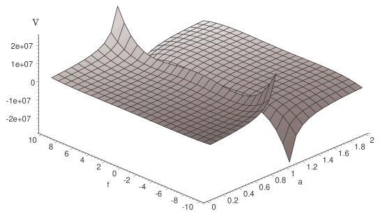
FIG. 1.: The shape of the potential in the condition of Re$f^{1}={\rm Re}f^{2}={\rm Im}f^{1}={\rm Im}f^{2}=f$, $\Lambda^{\prime}=1$ and $\xi^{(a)}=100$.

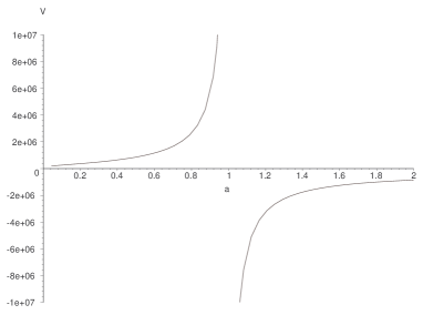
FIG. 2.: The slice of the potential along $f=0$ axis.

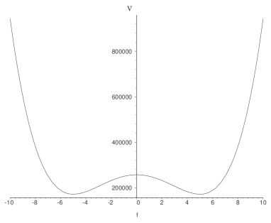
FIG. 3.: The slice of the potential along $a=0.1$ with $\xi^{(a)}=100$.

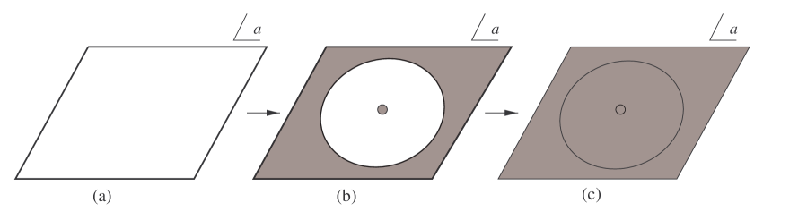
FIG. 4.: (a) Classical modulispace: No constraint for $a$. (b) Quantum moduli space: Shaded region ($a=0,a>\Lambda$) denotes the excluded region. (c) Quantum moduli with FI term: No allowed region. For clearly visualizing the situation, we describe these pictures as if $a$ takes a complex value, though its phase is unphysical.

REFERENCES

• [1] L. D. Landau, On the Quantum Theory of fields, in Niels Bohr and the Development of Physics, ed. by W. Pauli, Pergamon, London: (1955); L. D. Landau, A. Abrikosov and I. Khalatnikov, Nuovo Ciment, Supplement, 3 (1956) 80.
• [2] V. A. Miransky, Phys. Lett. 91B (1980) 421; P. I. Fomin, V. P. Gusynin, V. A. Miransky and Yu. A. Sitenko, Riv. Nuov. Cim. 6 (1983) 1; V. A. Miransky, Nuov. Cim. 90A (1985), 149.
• [3] W. A. Bardeen, C. N. Leung and S. T. Love, Phys. Rev. Lett. 56 (1986) 1230; C. N. Leung, S.T. Love and W.A. Bardeen, Nucl. Phys. B273 (1986) 649.
• [4] K.-I. Kondo, H. Mino and K. Yamawaki, Phys. Rev. D39 (1989) 2430.
• [5] T. Nonoyama, T. B. Suzuki, K. Yamawaki, Prog. Theor. Phys. 811 (1989) 1238.
• [6] J. B. Kogut. E. Dagotto and A. Kocic, Nucl. Phys. B317 (1989) 253; J. B. Kogut. E. Dagotto and A. Kocic, Nucl. Phys. B317 (1989) 271.
• [7] M. Göckeler, R. Horsey, P. Rakow, G. Schierholz and R. Sommer, Nucl. Phys B371 (1992) 713.
• [8] N. Seiberg, Phys. Lett. B318 (1993), 469; N. Seiberg, Phys. Rev. D49 (1994), 6857; K. Intriligator, R.G. Leigh and N. Seiberg, Phys .Rev. D50 (1994) 1092.
• [9] N. Seiberg and E. Witten, Nucl. Phys. B426 (1994) 19.
• [10] N. Seiberg and E. Witten, Nucl. Phys. B431 (1994) 484.
• [11] A. Masiero and G. Veneziano, Nucl. Phys. B249 (1985) 593.
• [12] O. Aharony, J. Sonnenshein, M. E. Peskin and S. Yankielowicz, Phys. Rev. D52 (1995) 6157.
• [13] E. D’Hoker, Y. Mimura and N. Sakai, Phys. Rev. D54 (1996) 7724.
• [14] N. Evans, S. D. H. Hsu, M. Schwetz, Phys. Lett. B355 (1995) 475; N. Evans, S. D. H. Hsu, M. Schwetz, Nucl. Phys. B456 (1995) 205.
• [15] S. P. Martin and J. D. Wells, Phys. Rev. D58 (1998) 115013.
• [16] L. Alvarez-Gaume and M. Marino, Int. J. Mod. Phys. A12 (1997) 975. L. Alvarez-Gaume, J. Distler, C. Kounnas and M. Marino, Int. J. Mod. Phys. A11 (1996) 4745.
• [17] P. Fayet and J. Iliopoulos. Nucl. Phys. B113 (1976) 135.
• [18] A. El. Hassouni, T. Lhallabi, E. G. Oudrhiri-Safiani and E. H. Saidi, Class. Quantum Grav. 5 (1988) 287.
• [19] E. A. Ivanov, S. V. Ketov and B. M. Zupnik, Nucl. Phys. B509 (1998) 53.
• [20] R. Grimm, M. Sohniu and J. Wess, Nucl. Phys. B133 (1978) 275.
• [21] P. Fayet, Nucl. Phys B113 (1976) 135; M. Sohnius, Nucl. Phys. B138 (1978) 109.
• [22] P. S. Howe, K. S. Stelle and P. K. Townsend, Nucl. Phys. B236 (1984) 125
• [23] A. Galperin, E. Ivanov, S. Kalitzin, V. Ogievetsky and E. Sokatchev, Class. Quantum Grav. 1 (1984) 469; A. Galperin, E. Ivanov, V. Ogievetsky and E. Sokatchev, Class. Quantum Grav. 2 (1985) 601; 617.
• [24] S. V. Ketov, Phys. Lett. 399B (1997) 83.