Non-BPS States and Branes in String Theory

Ashoke Sen

Mehta Research Institute of Mathematics

and Mathematical Physics

Chhatnag Road, Jhoosi, Allahabad 211019, INDIA

Abstract

We review the recent developments in our understanding of non-BPS states and branes in string theory. The topics include 1) construction of unstable non-BPS D-branes in type IIA and type IIB string theories, 2) construction of stable non-BPS D-branes on various orbifolds and orientifolds of type II string theories, 3) description of BPS and non-BPS D-branes as tachyonic soliton solutions on brane-antibrane pair of higher dimension, and 4) study of the spectrum of non-BPS states and branes on a system of coincident D-brane $-$ orientifold plane system. Some other related results are also discussed briefly.

1 Introduction

In this article I shall review the recent progress in our understanding of stable non-BPS branes and states in string theory. These lectures will be based mainly on refs.[1, 2, 3, 4, 5, 6, 7, 8, 9, 10]. We shall work in the convention $\hbar=1$, $c=1$, and $\alpha^{\prime}=1$ (string tension=$(2\pi)^{-1}$) unless mentioned otherwise.

Let us begin with some motivation for studying non-BPS branes. There are several reasons:

1. Stable non-BPS states and branes are very much part of the spectrum of string theory, and our understanding of string theory remains incomplete without a knowledge of these states.

2. Stable non-BPS states are the simplest objects whose masses are not protected by supersymmetry, and yet are calculable in different limits of the string coupling. Hence studying the spectrum of these states in these different limits might provide new insight into what happens at finite string coupling.

3. A system of coincident non-BPS D-branes typically has, as its world-volume theory, a non-supersymmetric gauge theory. Thus they may be useful in getting results about non-supersymmetric field theories from string theory, in the same way that a configuration of supersymmetric branes can be used to study non-perturbative aspects of supersymmetric gauge theories.

4. Non-BPS branes may be relevant for constructing string compactification with broken supersymmetry.

The plan of this article is as follows. In section 2 we shall discuss the construction of unstable non-BPS D-branes in type IIA and type IIB string theories. Whereas type IIA (IIB) string theory admits stable BPS branes of even (odd) dimensions, we shall see that they also admit unstable non-BPS branes of odd (even) dimensions. In section 3 we shall show how on certain orientifolds / orbifolds of type II string theories these non-BPS branes may give rise to stable non-BPS states and branes. The main point here will be to note that under this orbifolding / orientifolding operation the tachyonic mode responsible for the instability of the non-BPS brane gets projected out. The resulting brane is free from tachyonic mode and hence is stable. In section 4 we shall discuss the interpretation of the non-BPS branes in type IIA and IIB string theories as tachyonic kink solution on a BPS D-brane - anti-D-brane pair of one higher dimension in the same theory. We shall also show how the BPS D-brane (anti-D-brane) can be regarded as a tachyonic kink (anti-kink) solution on a non-BPS D-brane of one higher dimension. This gives a set of descent relations between BPS and non-BPS D-branes of type II string theories, and form the basis of identifying the D-brane charge with elements of K-theory[7, 9, 11, 12, 13, 14, 15, 16]. Since the actual proof of these relations is technically somewhat complicated, we postpone the details to the appendix.

In section 5 we discuss the spectrum of stable non-BPS states and branes on a coincident D-brane and orientifold plane system. The masses (tensions) of these states (branes) can be calculated in the strong coupling limit using various duality symmetries of string theory. Although for each system we use a completely different method for finding the spectrum, the final spectrum of non-BPS states and branes on a D-$p$-brane $-$ orientifold $p$-plane system exhibits an unusual regularity as a function of $p$. Whether this signifies any deep aspect of string theory remains to be seen. Since the only similarity between these systems is in their weak coupling perturbation expansion, we suspect that the strong coupling result may be governed by large order behaviour of this perturbation expansion. Finally in section 6 we discuss some related developments in this subject. This includes a discussion of some other non-BPS branes in type I string theory, the relationship between K-theory and D-brane charges, and the application of boundary state formalism in the study of non-BPS D-branes. We end with a discussion of some open questions.

2 Unstable Non-BPS D-branes in Type II String Theories

2.1 BPS D-branes in type II string theories

Figure 1: Open strings ending on a BPS D-brane.

Let us begin by reviewing what we know about BPS D-branes in type IIA/IIB string theories[17]. The defining property of the D-brane is that fundamental strings can end on a D-brane as shown in Fig.1, although type II string theories in the bulk only contains closed string states without any end. The open strings with ends on the D-brane can be interpreted as the dynamical modes of the D-brane. In order to compute the spectrum of these open string states with ends on the D-brane, we impose Dirichlet boundary condition on the open string coordinates along directions transverse to the D-brane, and Neumann boundary condition along directions parallel to the brane world-volume (including time). A D-brane with $p$ tangential spatial directions is called a D-$p$-brane.

Let us now list some of the properties of D-branes in type II string theories which will be useful to us later.

• Type IIA (IIB) string theory admits BPS D-$2p$-brane (D-$(2p+1)$-brane) which are invariant under half of the space-time supersymmetry transformations of the theory.

• A D-$p$-brane is charged under a $(p+1)$-form gauge field arising in the Ramond-Ramond (RR) sector of the theory.

• These BPS D-branes are oriented. D-branes of opposite orientation carry opposite RR charge and will be called anti-D-branes ($\bar{\rm D}$-branes).

Figure 2: Open strings living on a coincident D-brane anti-D-brane pair. Although for clarity we have displayed the brane and the anti-brane to be spatially separated, we shall analyse the case where they coincide.

Next we shall review properties of coincident D-brane $-$ ${\bar{\rm D}}$-brane pair shown in Fig.2. They are as follows:

• Spectrum of open strings living on the world-volume contains four different sectors. These four sectors can be labelled by $2\times 2$ Chan Paton (CP) factors:

  $$(a):\quad\pmatrix{0&0\cr 0&1},\qquad(b):\quad\pmatrix{1&0\cr 0&0}$$

  $$(c):\quad\pmatrix{0&0\cr 1&0},\qquad(d):\quad\pmatrix{0&1\cr 0&0}\,.$$ (2.1)

• GSO projection: Physical states in sectors (a) and (b) should have $(-1)^{F}=1$ whereas those in sectors (c) and (d) should have $(-1)^{F}=-1$. Here $F$ denotes the world-sheet fermion number carried by the state. We use the convention that the $(-1)^{F}$ eigenvalue of the Neveu-Schwarz (NS) sector ground state is $-1$. The GSO projection rule follows from the observation that the closed string exchange interaction between a D-brane and a ${\bar{\rm D}}$-brane and that between a pair of D-branes have the same sign for NSNS sector closed string exchange and opposite sign for RR sector closed string exchange. In the open string channel this corresponds to replacing the GSO projection operator ${1+(-1)^{F}\over 2}$ for DD strings by ${1-(-1)^{F}\over 2}$ for D${\bar{\rm D}}$ strings.

• Since the NS sector ground state has $(-1)^{F}=-1$, it survives the GSO projection in sectors (c) and (d) and gives tachyonic excitations with[18, 19, 20, 21, 22]

  $$m^{2}=-(1/2)\,.$$ (2.2)

  Since the tachyon comes from two different sectors it is a complex scalar field.

• Although individually the D-brane as well as the ${\bar{\rm D}}$-brane is invariant under half of the space-time supersymmetry transformations, the combined system breaks all supersymmetries.

We shall now study the action of $(-1)^{F_{L}}$ on the coincident D-brane $-$ ${\bar{\rm D}}$-brane system, where $F_{L}$ denotes the contribution to the space-time fermion number from the left-moving sector of the string world-sheet. $(-1)^{F_{L}}$ is known to be an exact symmetry of type IIA and type IIB string theories. Acting on the closed string Hilbert space, it changes the sign of all the states on the left-moving Ramond sector, but does not change anything else. Thus it has trivial action on the world-sheet fields. From this definition it follows that the space-time fields originating in the Ramond-Ramond (RR) sector of the world-sheet change sign under $(-1)^{F_{L}}$. Since D-branes are charged under RR field, it follows that $(-1)^{F_{L}}$ must take a D-brane to a ${\bar{\rm D}}$-brane. Thus a single D-brane or a single ${\bar{\rm D}}$-brane is not invariant under $(-1)^{F_{L}}$, but a coincident D-brane $-$ ${\bar{\rm D}}$-brane system is invariant under $(-1)^{F_{L}}$. Hence it makes sense to study the action of $(-1)^{F_{L}}$ on the open strings living on this system, which is what we shall do now.

We begin with the observation that since $(-1)^{F_{L}}$ has no action on the world-sheet fields, we only need to study its action on the CP factors. Since $(-1)^{F_{L}}$ exchanges D-brane with ${\bar{\rm D}}$-brane, it acts on the CP matrix $\Lambda$ as

$$\Lambda\to\sigma_{1}\Lambda(\sigma_{1})^{-1}\,,$$ (2.3)

where

$$\sigma_{1}=\pmatrix{0&1\cr 1&0}\,.$$ (2.4)

This shows that states with CP factors $I$ and $\sigma_{1}$ are even under $(-1)^{F_{L}}$, whereas those with CP factors $\sigma_{3}$ and $i\sigma_{2}$ are odd. (We could replace $\sigma_{1}$ by $\sigma_{2}$ in (2.3), but this just amounts to a change in convention.)

2.2 Non-BPS D-branes in type II string theories

We are now ready to define a non-BPS D-$2p$-brane of type IIB string theory[8]. This is done by following the steps listed below.

• We start with a D-$2p$ $-$ ${\bar{\rm D}}$-$2p$-brane pair in type IIA string theory and take the orbifold of this configuration by $(-1)^{F_{L}}$.

• In the bulk, modding out IIA by $(-1)^{F_{L}}$ gives IIB.

• Acting on the open strings living on the D-${\bar{\rm D}}$-brane world-volume, $(-1)^{F_{L}}$ projection keeps states with CP factors $I$ and $\sigma_{1}$ and throws out states with CP factors $\sigma_{3}$ and $i\sigma_{2}$.

This defines a non-BPS D-$2p$-brane of type IIB string theory. In order to see that it describes a single object rather than a pair of objects, we simply note that before the projection the degree of freedom of separating the two branes reside in the sector with CP factor $\sigma_{3}$. Since states in the CP sector $\sigma_{3}$ are projected out, we lose the degree of freedom of separating the brane antibrane pair away from each other. Similarly, starting from a D-$(2p+1)$-brane ${\bar{\rm D}}$-$(2p+1)$-brane pair of IIB, and modding it out by $(-1)^{F_{L}}$, we can define a non-BPS $(2p+1)$-brane of IIA. Thus type IIB string theory contains BPS D-branes of odd dimension and non-BPS D-branes of even dimension, whereas type IIA string theory contains BPS D-branes of even dimension and non-BPS D-branes of odd dimension.

Let us now list some of the properties of the non-BPS D-$2p$-brane of type IIB string theory. (Similar results also hold for the non-BPS D-$(2p+1)$-brane of type IIA string theory.) These properties follow from their definition, and properties of coincident brane-antibrane pair reviewed earlier.

• Excitations on its world-volume are open strings with Dirichlet boundary condition on the $(9-2p)$ transverse directions, and Neumann boundary condition on $2p+1$ tangential directions (including time).

• These open strings carry Chan Paton factors $I$ or $\sigma_{1}$.

• Physical states with CP factor $I$ has $(-1)^{F}=1$ and physical states with CP factor $\sigma_{1}$ has $(-1)^{F}=-1$. (Note again that $F$ denotes world-sheet fermion number.)

• The NS sector ground state carrying CP factor $\sigma_{1}$ has $(-1)^{F}=-1$ and hence is physical. Thus there is a tachyonic mode with

  $$m^{2}=-{1\over 2}\,.$$ (2.5)

• Since tachyon comes from only one sector, it is a real scalar field.

• The tension of the non-BPS D-$2p$-brane of type IIB string theory is given by:

  $$(2\pi)^{-2p}(\sqrt{2}/g)\,,$$ (2.6)

  where $g$ denotes the coupling constant of the string theory. This property can be derived by taking into account the effect of modding out by $(-1)^{F_{L}}$, and the fact that the original brane-antibrane system before $(-1)^{F_{L}}$ modding had a tension equal to

  $$(2\pi)^{-2p}(2/g)\,.$$ (2.7)

  Similarly, the tension of a non-BPS D-$(2p+1)$-brane of type IIA string theory is given by

  $$(2\pi)^{-(2p+1)}(\sqrt{2}/g)\,.$$ (2.8)

One can also derive the spectrum of open strings with one end on the non-BPS brane and other end on a BPS brane, but we shall not discuss it here.

2.3 BPS D-branes from non-BPS D-branes

Let us now consider the effect of modding out a non-BPS D-$2p$-brane of IIB by $(-1)^{F_{L}}$, where $(-1)^{F_{L}}$ now denotes the corresponding symmetry of the type IIB string theory[8]. In the bulk, modding out type IIB string theory by $(-1)^{F_{L}}$ gives us back a type IIA string theory. The question we shall be interested in is: what happens to the D-$2p$-brane after this modding? This question makes sense as the non-BPS D-brane does not carry any RR charge and hence is invariant under the action of $(-1)^{F_{L}}$. In order to answer this question we need to study the action of $(-1)^{F_{L}}$ on the open string states living on the D-$2p$-brane. As before $(-1)^{F_{L}}$ does not act on the world-sheet fields, but acts only on the CP factors. Thus we need to find the action of $(-1)^{F_{L}}$ on CP factors. This is done with the help of the following observations:

Figure 3: The disk amplitude for two point function of the graviton and translation mode of the D-brane.

• There is a non-zero two point function of the graviton $g_{m\mu}$ from the closed string sector and the translation modes $X^{m}$ of the D-$2p$-brane originating in the CP sector $I$ of the form:

  $$\eta^{\mu\nu}g_{m\mu}\partial_{\nu}X^{m}\,,$$ (2.9)

  where $m$ denotes a direction transverse to the brane and $\mu,\nu$ denote directions tangential to the brane. This coupling follows from expanding the Dirac-Born-Infeld action on the brane world-volume around the configuration of a flat brane in a flat space-time background. This can also be seen by computing a disk amplitude with a graviton vertex operator inserted at the center of the disk, and the tachyon vertex operator inserted at the boundary of the disk, as shown in Fig.3. Since the graviton is even under $(-1)^{F_{L}}$, this shows that states with CP factor $I$ must also be even under $(-1)^{F_{L}}$.

  

  Figure 4: The disk amplitude for the two point function of the tachyon and the RR sector $2p$-form gauge field. The dotted line denotes the $(-1)^{F_{L}}$ cut extending from the RR vertex operator to the disk boundary.

• There is a non-zero two point function of the RR-sector $2p$-form gauge field $A^{(2p)}$ from the closed string sector and the tachyonic mode $T$ of the D-$2p$-brane originating in the CP sector $\sigma_{1}$ of the form:

  $$\int A^{(2p)}\wedge dT\,.$$ (2.10)

  This can be seen by computing the disk amplitude with a RR-sector gauge field vertex operator inserted at the center of the disk, and the tachyon vertex operator inserted at the boundary, as shown in Fig.4. The fact that this amplitude is non-zero may seem surprising, as the tachyon vertex operator carries a CP factor $\sigma_{1}$, and there seems to be no other CP factor inserted at the boundary of the disk. However, since the RR sector states in type IIB string theory appear in the twisted sector when we regard type IIB string theory as type IIA string theory modded out by $(-1)^{F_{L}}$, there is a cut extending from the RR sector vertex operator at the center all the way to the boundary of the disk. At the point where the cut hits the boundary we need to insert an extra factor of $\sigma_{1}$, since $(-1)^{F_{L}}$ action on the CP factors correspond to conjugation by $\sigma_{1}$. This gives a total of two factors of $\sigma_{1}$ on the disk boundary and makes the amplitude non-vanishing. From this it follows that since RR-sector fields are odd under $(-1)^{F_{L}}$, states with CP factor $\sigma_{1}$ are also odd under $(-1)^{F_{L}}$.

The net result of this analysis is that states with CP factor $I$ are $(-1)^{F_{L}}$ even and states with CP factor $\sigma_{1}$ are $(-1)^{F_{L}}$ odd. Thus under modding out by $(-1)^{F_{L}}$, only states with CP factor $I$ survive the projection. As we have already seen before, GSO projection requires these states to be even under $(-1)^{F}$. Thus the spectrum is identical to that of open strings living on a BPS D-$2p$-brane of IIA, and we conclude that the non-BPS D-$2p$-brane of type IIB string theory, modded out by $(-1)^{F_{L}}$, gives a BPS D-$2p$-brane of type IIA string theory.

Figure 5: Relationship between BPS and non-BPS D-branes in type II string theories. The horizontal arrow represents the effect of modding out the theory by $(-1)^{F_{L}}$.

The results of this section have been summarized in Fig.5. There is also a similar relation with IIA $\leftrightarrow$ IIB and $(2p)\rightarrow(2p+1)$.

3 Stable Non-BPS D-branes on Type II Orbifolds and Orientifolds

Although we have constructed non-BPS D-branes in type IIA/IIB string theory in the last section, they are all unstable due to the presence of the tachyonic mode. As we shall discuss in section 4, if the tachyon condenses to its minimum, then the configuration is indistinguishible from the vacuum[3]. Thus it is natural to ask: what is the use of such a D-brane?

In this section we shall show that although they are unstable in type IIA/IIB string theory, we may get stable non-BPS D-branes in certain orbifolds/orientifolds of IIA/IIB if the tachyonic mode is projected out under this operation. We shall illustrate this through two examples.

3.1 Type I D-particle

Let us consider the following construction:

• Start with the non-BPS D0-brane (D-particle) of type IIB as defined in the last section.

• Mod out the configuration by the world-sheet parity transformation $\Omega$.

The result can be described as a non-BPS D-particle of type I string theory, since in the bulk type IIB string theory modded out by $\Omega$ gives a type I string theory. The crucial question is: is this D-particle stable? Or equivalently we may ask: is the tachyonic mode on the type IIB D-particle odd under $\Omega$? The answer to this question follows from eq.(2.10) for $p=0$, i.e. that the two point function of the tachyonic mode on the D-particle world-volume and the RR sector scalar field $\phi$ of type IIB string theory is non-vanishing. Since the field $\phi$ is known to be odd under $\Omega$, we conclude that the tachyonic mode of the D-particle is also odd under $\Omega$. Thus it is projected out in type I string theory. In other words, the type I D-particle is stable[6]!

The spectrum of open strings on type I D-particle also includes open strings with one end on the D-particle and the other end on any one of the 32 nine branes which are present in type I string theory. The Ramond sector states from this sector can be shown to give rise to 32 massless fermionic zero modes living on the D0-brane. Quantization of these zero modes gives rise to a ground state which transforms in the spinor representation of the type I gauge group SO(32). This also gives an additional explanation of the stability of the D-particle. Since all perturbative states of type I string theory are in the scalar conjugacy class of SO(32), and since a spinor state cannot decay into states in the scalar conjugacy class, the D-particle is prevented from decaying into perturbative string states due to charge conservation.

If we consider two or more coincident D-particles in type I string theory, then there are also possible tachyonic modes coming from open strings with two ends on two different D-particles. It turns out that the $\Omega$ projection does not remove all the tachyonic modes from these sectors, and two or more coincident D-particles describe an unstable system. This is consistent with the observation that two particles in the spinor representation of SO(32) can combine and annihilate into perturbative string states, as there is no conservation law preventing this process.

The existence of the type I D-particle is also relevant for testing the conjectured duality between type I and heterotic string theory[24, 25, 26, 27]. SO(32) heterotic string theory contains states in the perturbative spectrum which transform in the spinor representation of SO(32). These states are massive, and non-BPS. But the lightest state belonging to the spinor representation of SO(32) is stable at all values of the coupling, as they cannot decay into anything else. Thus these states must also exist in the strong coupling limit of the SO(32) heterotic string theory, which is nothing but the weakly coupled type I string theory. The type I D-particles provide explicit realization of these states.

It is instructive to compare the mass formulae for these SO(32) spinor states at the two extreme ranges of the coupling constant. We shall use the variables of the heterotic string theory to express this mass formula at the two ends. For small heterotic coupling $g_{H}$, the perturbative mass formula in the heterotic string theory holds:

$$\sqrt{T_{H}}\,(a_{0}+a_{1}\,g_{H}^{2}+a_{2}\,g_{H}^{4}+\ldots)\,,$$ (3.1)

where $T_{H}$ is the heterotic string tension, and $a_{i}$ are numerical coefficients. $a_{0}$ is computed at tree level of heterotic string theory, whereas $a_{m}$ is computed at $m$-loop order.

For large heterotic coupling we can use the description of this state as type I D-particle to compute its mass. As we saw earlier, this has mass of order $\sqrt{T_{I}}/g_{I}$, where $T_{I}$ and $g_{I}$ are the string tension and coupling constant respectively of the type I string theory. Using standard relationship between the heterotic and type I variables[24]

$$T_{I}=T_{H}g_{H}^{-1},\qquad g_{I}=g_{H}^{-1}\,,$$ (3.2)

we see that for large $g_{H}$ the mass of this state is proportional to:

$$\sqrt{T_{H}}(g_{H})^{1/2}\,.$$ (3.3)

It will be interesting to see if the perturbation expansion (3.1) contains any information about the large $g_{H}$ behaviour given in (3.3).

3.2 D-branes wrapped on non-supersymmetric cycles of K3 orbifold

In this section we shall discuss another example where the tachyonic mode of a non-BPS D-brane is projected out under an orbifolding operation[8]. We proceed as follows:

• Start with a non-BPS D-string of type IIA string theory wrapped on a circle along $x^{9}$ of radius $R_{9}$ and placed at $x^{i}=0$ for $1\leq i\leq 8$.

• Compactify three other directions $x^{6},x^{7},x^{8}$.

• Mod out the theory by a $Z_{2}$ transformation ${\cal I}_{4}$ which changes the sign of $x^{6},\ldots x^{9}$:

  $${\cal I}_{4}:\quad(x^{6},x^{7},x^{8},x^{9})\to(-x^{6},-x^{7},-x^{8},-x^{9})\,.$$ (3.4)

In the bulk this gives type IIA string theory on an orbifold K3. We shall now analyze the fate of the tachyon field on the D-string in this orbifold theory. Since the D-string lies along $x^{9}$, the tachyon field on its world-steet is a function of $x^{9}$ and time $t$. Again by considering a two point function between the tachyon and an RR sector gauge field, one can show that under the $Z_{2}$ transformation ${\cal I}_{4}$,

$$T(x^{9},t)\to-T(-x^{9},t)\,.$$ (3.5)

If we expand $T(x^{9},t)$ in its Fourier mode as:

$$T(x^{9},t)=\sum_{n}T_{n}(t)e^{inx^{9}/R_{9}}\,,$$ (3.6)

then under ${\cal I}_{4}$:

$$T_{n}(t)\to-T_{-n}(t)\,.$$ (3.7)

Thus

• $T_{0}$ is projected out.

• For $n\neq 0$ the combination $T_{n}-T_{-n}$ survives the projection under ${\cal I}_{4}$.

Since the effective mass² of $T_{n}-T_{-n}$ is given by

$$m_{n}^{2}=(n^{2}/R_{9}^{2})-(1/2)\,,$$ (3.8)

we see that there is no tachyon in the spectrum for

$$R_{9}\leq\sqrt{2}\,.$$ (3.9)

There are also possible tachyonic modes from open string states stretched between the original D-string and its image under translation along $x^{6}$, $x^{7}$ or $x^{8}$. Demanding that there are no tachyonic modes from these sectors we also get

$$R_{8}\geq{1\over\sqrt{2}},\quad R_{7}\geq{1\over\sqrt{2}},\quad R_{6}\geq{1\over\sqrt{2}}\,.$$ (3.10)

Figure 6: The D0-${\bar{\rm D}}$0 brane configuration obtained by marginal deformation of the non-BPS D-string wrapped along $x^{9}$.

The net result of this analysis is that we have a stable non-BPS state in type IIA string theory on $T^{4}/{\cal I}_{4}$ in the range of parameters described in (3.9), (3.10). The next question would be: what is the interpretation of this state? There are many ways to answer the question; we shall explain it by studying the physics at the critical radius $R_{9}=\sqrt{2}$. At this radius $T_{\pm 1}$ are massless modes. In fact one can show that the potential for $(T_{1}-T_{-1})$ vanishes identically. Thus $(T_{1}-T_{-1})$ denotes an exactly marginal deformation of the boundary conformal field theory (CFT) describing the D-brane. We can study this deformation using CFT techniques. We shall only quote the result here (see section 4, the appendix and ref.[8] for some of the details). It turns out that this marginal deformation takes the non-BPS D-string of IIA to a D$0$-${\bar{\rm D}}$0-brane pair situated at the two fixed points $x^{9}=0$ and $x^{9}=\pi R_{9}$ respectively as shown in Fig.6.

So far what we have described could have been done even before modding out the theory by ${\cal I}_{4}$. Let us now study the result of modding out this configuration by ${\cal I}_{4}$. It was shown in ref.[28] that after modding out by ${\cal I}_{4}$ a $D0$-brane at $x^{9}=0$ can be interpreted as a D2-brane of type IIA string theory, wrapped on the supersymmetric 2-cycle[29] associated with the fixed point of ${\cal I}_{4}$ at $x^{9}=0$. A similar interpretation can be given for the ${\bar{\rm D}}$0-brane at $x^{9}=\pi R_{9}$. Thus in the orbifold theory the marginal perturbation by $(T_{1}-T_{-1})$ at $R_{9}={\sqrt{2}}$ takes the original non-BPS state to a pair of D2-branes, wrapped on the 2-cycles associated with the fixed points at $x^{9}=0$ and $x^{9}=\pi R_{9}$ respectively. This suggests that the original configuration is a D-2-brane of IIA wrapped simultaneously on both these 2-cycles. This represents a D2-brane wrapped on a non-supersymmetric 2-cycle.

Before the projection, the mass of the wrapped non-BPS D-string is given by $(\sqrt{2}R_{9}/g)$, whereas the sum of the masses of the D0-${\bar{\rm D}}$0 pair is given by $(2/g)$. Modding out by ${\cal I}_{4}$ reduces the mass of each state to half its original value. By comparing the masses of the various (wrapped) branes we arrive at the following picture:

• At the critical radius the D-2-brane wrapped on the non-supersymmetric cycle is degenerate with the pair of D-2-branes wrapped on the supersymmetric cycles.

• Below the critical radius the D-2-brane wrapped on the non-supersymmetric cycle is lighter than the pair of D-2-branes wrapped on the two supersymmetric cycles. Hence this wrapped brane is stable.

• Above the critical radius the D-2-brane wrapped on the non-supersymmetric cycle is heavier than the pair of D-2-branes wrapped on the two supersymmetric cycles. As a result this wrapped brane is unstable against decay into a pair of supersymmetric brane configurations.

This construction can be generalized to describe a $(2p+2)$-brane ($(2p+1)$-brane) of IIA (IIB) wrapped on a non-supersymmetric cycle of K3. Using this procedure one can also construct examples of D-branes wrapped on non-BPS 2- and 3-cycles of Calabi-Yau manifolds. These generalizations have been discussed in ref.[8].

Before concluding this discussion we note that the world-volume theory of $N$ coincident branes of this type gives rise to a non-supersymmetric U(N) gauge theory. This might be useful in solving non-supersymmetric field theories via branes.

4 D-branes as Tachyonic Kink Solutions

4.1 Non-BPS D-brane as tachyonic kink on the brane-antibrane pair

Figure 7: The tachyon potential on D-brane $-$ ${\bar{\rm D}}$-brane pair.

In this section we shall give an alternative construction of the non-BPS D-branes discussed in section 2[2, 5]. Let us start with a coincident pair of D-$2p$ $-$ ${\bar{\rm D}}$-$2p$ branes ($p\geq 1$) of type IIA string theory. As discussed in section 2, there is a complex tachyon field $T$ living on the world-volume of this system. This reflects the fact that $T=0$ is the maximum of the tachyon potential $V(T)$ obtained after integrating out all other massive modes on the world-volume. There is a U(1)$\times$U(1) gauge field living on the world-volume of the brane-antibrane system, and the tachyon picks up a phase under each of these U(1) gauge transformations. As a result, $V(T)$ is a function only of $|T|$, and the minimum of the potential occurs at $T=T_{0}e^{i\theta}$ for some fixed $T_{0}$ but arbitrary $\theta$, as shown in Fig.7. As we shall argue shortly, at the minimum, the sum of the tension of the D-brane ${\bar{\rm D}}$-brane pair and the (negative) potential energy of the tachyon is exactly zero[3] i.e.,

$$2T_{D}+V(T_{0})=0\,,$$ (4.1)

where $T_{D}$ is the D-brane tension. This shows that the tachyonic ground state $T=T_{0}$ is indistinguishible from the vacuum, since it carries neither any charge nor any energy density.

Figure 8: Tachyonic kink solution on the brane-antibrane pair.

But now, instead of considering tachyonic ground state, let us consider a tachyonic kink solution. For this, consider the minimum energy configuration with the following properties:

• $Im(T)=0$.

• $Re(T)$ independent of time and $(2p-1)$ of the $2p$ spatial coordinates.

• $Re(T)$ depends on the remaining spatial coordinate $x$ such that

  $$\displaystyle T(x)\to T_{0}\quad \quad x\to\infty,$$ as

  $$T(x)\to-T_{0}\quad \quad x\to-\infty\,.$$ as (4.2)

This has been shown in Fig.8. From this it is clear that as $x\to\pm\infty$ the solution goes to vacuum configuration. Thus the energy density is concentrated around a $(2p-1)$ dimensional subspace, and the solution describes a $(2p-1)$-dimensional brane. We now claim that this $(2p-1)$-brane associated with the tachyonic kink solution on the brane-antibrane pair is identical to the non-BPS D-$(2p-1)$-brane of IIA.

Note that $V(T)$ cannot be explicitly calculated. Thus one might ask how one could show the equivalence between the non-BPS D-brane described in section 2 and the tachyonic kink on the brane $-$ antibrane pair described here. This will be discussed in some detail in the appendix; but here we shall describe the outline of the proof.

• There is a marginal deformation involving bulk and boundary operators which interpolates between the $T=0$ configuration and the kink solution.

• One can study the fate of the CFT describing the brane-antibrane pair under this marginal deformation.

• The end result turns out to be a CFT which is identical to the CFT describing the non-BPS D-brane.

One can also give an intuitive understanding of why a tachyonic kink should behave like a D-brane. For this note that far away from the kink (large $|x|$) the configuration represents the vacuum, and hence strings cannot end there. On the other hand, on the subspace $x=0$, the tachyon field vanishes, and hence we expect the configuration to behave in a way that a D-brane $-$ ${\bar{\rm D}}$-brane pair would have behaved in the absence of tachyon vev, i.e. open strings should be able to end there. Thus the tachyonic kink should at least qualitatively behave as a D-brane located at $x=0$.

Note that the manifold ${\cal M}$ describing the minimum of the tachyon potential is a circle $S^{1}$. In order to get a topologically stable kink solution, we need $\pi_{0}({\cal M})\neq 0$. But $\pi_{0}(S^{1})=0$ since $S^{1}$ is connected. Thus the kink is not topologically stable. Indeed it has tachyonic mode correponding to the freedom of changing $T$ at $x\to\infty$ to $T_{0}e^{i\theta}$. As $\theta\to\pi$ we get back the vacuum configuration, since $T\to-T_{0}$ as $x\to\pm\infty$ in this case. This however is completely consistent with the identification of this kink solution with the non-BPS D-$(2p-1)$-brane of type IIA string theory, since, as we have seen earlier, the latter also has a tachyonic mode living on it. The tachyonic mode on the kink solution can be identified as the tachyonic mode on the non-BPS D-$(2p-1)$-brane of IIA discovered in section 2.

Before we move on to the next subject, let us give an argument in favour of eq.(4.1). For this, note that if (4.1) had not been true, then the tachyonic kink solution described here will not have a finite energy per unit $(2p-1)$-volume, since the energy density, integrated along the transverse direction (denoted by $x$ in eq.(• ‣ 4.1)) would give infinite answer. On the other hand from the analysis of section 2 we certainly know that a non-BPS D-$(2p-1)$ brane of type IIA string theory has finite tension. Thus once we establish the equivalence of the tachyonic kink solution and the non-BPS D-brane (as will be discussed in the appendix), it automatically establishes eq.(4.1).

4.2 The BPS D-brane as the tachyonic kink on the non-BPS D-brane

Figure 9: The tachyon potential on the non-BPS D-brane

We can now continue one step further. Let us start with a non-BPS D-$(2p-1)$-brane of IIA. As was discussed in section 2, it has a real tachyon $\widetilde{T}$. By studying the disk amplitude it can be easily seen that there is a $Z_{2}$ symmetry on the world-volume of this non-BPS D-brane under which $\widetilde{T}$ (and all other modes originating in the CP sector $\sigma_{1}$) changes sign. Let $\pm\widetilde{T}_{0}$ be the minimum of the tachyon potential $\widetilde{V}(\widetilde{T})$ obtained after integration out the other massive modes, as shown in Fig.9. Again one can argue that:

$$\widetilde{V}(\widetilde{T}_{0})+\widetilde{T}_{D}=0\,,$$ (4.3)

where $\widetilde{T}_{D}$ is the tension of the non-BPS D-brane. We now consider a kink solution on this D-$(2p-1)$-brane world-volume such that:

Figure 10: Tachyonic kink solution on a non-BPS D-brane.

• $\widetilde{T}$ is independent of time as well as $(2p-2)$ of the spatial coordinates.

• It depends on the remaining world-volume coordinate $y$ such that:

  $$\displaystyle\widetilde{T}(y)\to\widetilde{T}_{0}\quad \quad y\to\infty,$$ as

  $$\widetilde{T}(y)\to-\widetilde{T}_{0}\quad \quad y\to-\infty\,.$$ as (4.4)

This configuration has been shown in Fig.10. By the same argument as in the previous subsection, this describes a $(2p-2)$ dimensional brane. We shall show in the appendix that this can be identified as the BPS D-$(2p-2)$ brane of type IIA string theory. The analysis is again based on finding a series of marginal deformations involving bulk and boundary operators which connect the $\widetilde{T}=0$ configuration of the non-BPS D-$(2p-1)$ brane to a solution representing a kink-antikink pair, and using conformal field theory techniques to show that this marginal deformation actually interpolates between the non-BPS D-$(2p-1)$-brane and a BPS D-$(2p-2)$-brane $-$ ${\bar{\rm D}}$-$(2p-2)$-brane pair.

Note that now the manifold $\widetilde{\cal M}$ describing the minimum of the tachyon potential consists of a pair of points $\pm\widetilde{T}_{0}$. Thus $\pi_{0}(\widetilde{\cal M})\neq 0$, and hence the kink is stable as is expected of a BPS D-brane. An argument similar to the one in the previous subsection can be used to give an intuitive explanation of why the kink should behave as a D-brane near $y=0$ but as vaccuum for large $|y|$. We can also explain the origin of the RR charge of the kink from the coupling (2.10) and the fact that $\partial_{y}T$ is non-zero at $y=0$. Since $\partial_{y}T$ has opposite sign for the anti-kink, this also shows that the anti-kink must represent the BPS ${\bar{\rm D}}$-$(2p-2)$ brane.

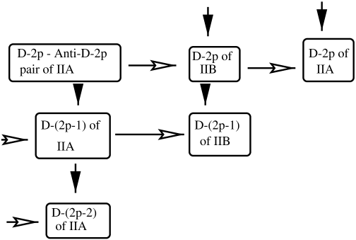
Figure 11: Descent relations among BPS and non-BPS D-branes in type II string theories. The horizontal arrows denote the effect of modding out by $(-1)^{F_{L}}$, and the vertical arrows denote the ffect of considering tachyonic kink solution.

The results of this section, combined with the results of section 2 leads to the set of ‘descent relations’ between BPS and non-BPS D-branes shown in Fig.11.

By combining the two main results of this section, we can also represent a BPS D-$p$-brane as a soliton (vortex) solution on the D-$(p+2)$-brane $-$ ${\bar{\rm D}}$-$(p+2)$-brane pair in the same theory[5, 7]. This construction is relevant for relating allowed D-brane charges to elements of the K-group of space-time[7].

5 Stable Non-BPS Branes on the D-brane $-$ Orientifold Plane System

5.1 Summary of the results

We have already introduced the notion of a D-$p$-brane in type II string theory. We now introduce the concept of an orientifold $p$-plane (O-$p$-plane)[31, 32]. For this we consider type II string theory on $R^{p+1}\times(R^{9-p}/{\cal I}_{9-p}\cdot\Omega\cdot g)$, where ${\cal I}_{9-p}$ reverses the sign of all the coordinates on $R^{9-p}$, $\Omega$ is the world-sheet parity transformation (L $\leftrightarrow$ R) and $g$ is identity for $(9-p)=4m$ or $(4m+1)$ and $g=(-1)^{F_{L}}$ for $(9-p)=(4m+2)$ or $(4m+3)$. One can show that ${\cal I}_{9-p}\cdot\Omega\cdot g$ is a symmetry transformation of order 2 in type IIA string theory if $p$ is even, and in type IIB string theory if $p$ is odd. The origin of $R^{9-p}$ will be called an orientifold $p$-plane. Thus type IIA (IIB) string theory contains orientifold $p$-planes of even (odd) dimensions.

Figure 12: Transverse section of the coincident D-$p$-brane $-$ O-$p$-plane system. Although for clarity we have shown the D-brane and the O-plane as separated in space, we shall analyze the case where they are on top of each other.

Our focus of attention in this section will be a system of parallel D-$p$-brane $-$ O-$p$-plane system. This corresponds to starting with a D-brane and its image under ${\cal I}_{9-p}\cdot\Omega\cdot g$, and then modding out the theory by ${\cal I}_{9-p}\cdot\Omega\cdot g$, as shown in Fig.12. The world volume theory of a Dirichlet $p$-brane (D-$p$-brane) on top of an orientifold $p$-plane (O-$p$-plane) has as its low energy limit an $N=4$ supersymmetric SO(2) gauge theory. The spectrum of stable states in this theory contains a massive non-BPS state carrying unit charge under this SO(2) gauge field. These arise from open strings stretched between the D-brane and its image. In the weak coupling limit these states have mass of the order of the string scale $m_{S}$ with corrections expressible as a perturbation series in the string coupling $g_{S}$:

$$m_{S}(K_{0}+K_{1}g_{S}+K_{2}g_{S}^{2}+\cdots)\,.$$ (5.1)

Here $K_{0},K_{1},K_{2},\ldots$ are numerical constants, with $K_{m}$ computed from a diagram with $m$ open string loops. Since the lowest mass state carrying SO(2) electric charge must be stable at all values of the string coupling, it makes sense to ask what would be the masses of these states in the strong coupling limit. This is one of the questions we address in this section. The answers were obtained in refs.[1, 2, 4, 5] and have been summarised in table 1.

$p$	mass	$C_{p}$
6	$C_{6}m_{S}g_{S}$	known
5	$C_{5}m_{S}(g_{S})^{1\over 2}$	known
4	$C_{4}m_{S}(g_{S})^{1\over 3}$	unknown
3	unknown	$-$

Table 1: Masses of electrically charged states on the D-$p$-brane O-$p$-plane system in the strong coupling limit.

In this table, the first column denotes the value of $p$, the second column denotes the mass of the lightest stable electrically charged state on the D-$p$-brane $-$ O-$p$-plane system, $C_{p}$ denotes a numerical constant, and the last column denotes whether the numerical constant $C_{p}$ is known or unknown at present. We have restricted $p$ in the range $3\leq p\leq 6$ due to the following reason. For $p\geq 7$, the dilaton does not go to a constant value asymptotically[34], and as a result the string coupling $g_{S}$ is not a well defined quantity. On the other hand, for $p\leq 2$, the self-energy of an electrically charged particle blows up due to the long range Coulomb field associated with the particle, and hence the mass of such a state is not a well defined quantity.

We shall review the arguments leading to these results in subsection 5.2. As we can see from this table, we still do not know the mass of the electrically charged particle on the D-3-brane $-$ O-3-plane system in the strong coupling limit. Although it may be somewhat premature to look for a pattern among three data points, we note that there seems to be some regularity in the dependence of this mass on $g_{S}$ for $4\leq p\leq 6$, namely it seems to go as

$$m_{S}(g_{S})^{1\over 7-p}\,.$$ (5.2)

Considering that for different values of $p$ these results are derived using very different techniques, one might wonder if there is a deeper lesson about strongly coupled string theory in this spectrum. Since the only feature that is common between different values of $p$ is the structure of weak coupling perturbation theory, it is tempting to speculate that the regularity of the strong coupling spectrum is a reflection of the regularity of the weak coupling perturbation theory as a function of $p$. In that case we can expect that the information about the strong couping result is somehow contained in the weak coupling perturbation theory, $-$ in particular in its large order behaviour.

Besides stable non-BPS states which are electrically charged under the SO(2), the brane world-volume theory also contains branes which are magnetically charged under the SO(2). On the D-$p$-brane O-$p$-plane system these are $(p-3)$ branes, and come from a D-$(p-2)$-brane, stretched between the brane and its image. Such configurations are allowed according to the rules of refs.[35, 36]. Naively, when the D-$p$-brane and its image coincide these stretched branes will have vanishing tension. But quantum corrections must give non-vanishing contribution to the tension, reflecting the fact that these are non-BPS branes. Unfortunately calculating tensions of these non-BPS branes in the weak coupling limit remains an open problem. However as we shall see in subsection 5.2, for every value of $p$ between 3 and 6, one can calculate the tensions of these non-BPS branes in the strong coupling limit. The answer has been summarized in table 2.

$p$	(tension)${}^{1\over(p-2)}$	$\widetilde{C}_{p}$
6	$\widetilde{C}_{6}m_{S}$	known
5	$\widetilde{C}_{5}m_{S}g_{S}^{-{1\over 6}}$	known
4	$\widetilde{C}_{4}m_{S}g_{S}^{-{1\over 3}}$	unknown
3	$\widetilde{C}_{3}m_{S}g_{S}^{-{1\over 2}}$	known

Table 2: Tensions of magnetically charged $(p-3)$-branes on the D-$p$-brane O-$p$-plane system in the strong coupling limit.

The first column in this table describes the value of $p$ as before. The second column represents the $(p-2)$-th root of the tension of the magnetically charged $(p-3)$-brane. This root is taken in order to make it into a quantity of mass dimension 1. $m_{S}$ and $g_{S}$ denote, as before, the square root of the fundamental string tension and the string coupling constant respectively, and $\widetilde{C}_{p}$ denote numerical constants. The last column shows that at present the coefficients $\widetilde{C}_{p}$ are known for $p=3$, 5 and 6, but not for $p=4$.

We again observe that there is a regularity in this spectrum. In particular the $(p-2)$-th root of the tension of the $(p-3)$-brane on the D-$p$-brane $-$ O-$p$-plane system goes as:

$$m_{S}(g_{S})^{{p\over 6}-1}\,.$$ (5.3)

Again it is natural to suspect that this reflects some deeper aspect of string theory which is not understood at present.

5.2 Strong coupling description of electrically charged states and magnetically charged branes

In this subsection we shall review the analysis leading to tables 1 and 2. We shall discuss each value of $p$ separately, since the strong coupling description of the D-$p$-plane $-$ O-$p$-plane system is different for each value of $p$.

$p=6$

In this case the system under study is a D6-brane on top of an O6-plane in type IIA string theory. The strong coupling description of this system is known to be M-theory on $R^{6,1}\times{\cal N}$, where $R^{6,1}$ is along the world-volume of the D6$-$O6 system, and ${\cal N}$ is the double cover of the Atiyah-Hitchin space[37] with a rescaled metric[38, 1]. Asymptotically, ${\cal N}$ locally looks like $R^{3}\times S^{1}$. The Planck mass $m_{p}$ of the M-theory, and the radius $R$ of this $S^{1}$ are related to $m_{S}$ and $g_{S}$ of type IIA string theory via the relations:

$$m_{p}=m_{S}(g_{S})^{-{1\over 3}},\qquad R=m_{S}^{-1}g_{S}\,.$$ (5.4)

The metric on ${\cal N}$ is given by

$$ds^{2}={R^{2}\over 4}ds_{AH}^{2}\,,$$ (5.5)

where $ds_{AH}^{2}$ is the standard Atiyah-Hitchin metric[37]. The SO(2) gauge field $A$ on the brane world-volume is related to the three form gauge field $C_{\mu\nu\rho}$ of M-theory as

$$C=\omega\wedge A+\cdots$$ (5.6)

where $\omega$ is the unique normalizable harmonic two form on ${\cal N}$[39, 40, 41], and $\cdots$ denotes terms involving other normalizable and non-normalizable differential forms on ${\cal N}$.

The topology as well as the metric on ${\cal N}$ is completely known. In particular ${\cal N}$ contains a non-contractible two cycle of minimal area $-$ called the bolt $-$ which has the property that the integral of the two form $\omega$ over the bolt is non-vanishing. From the relation (5.6) and the fact that a membrane is electrically charged under $C$, it follows that a membrane wrapped on the bolt will be electrically charged under $A$. In other words, the electrically charged stable non-BPS state on the world-volume of the D6$-$O6 system is described by the M-theory membrane wrapped on the bolt of ${\cal N}$[1]. The area of the bolt is equal to $\pi^{3}R^{2}$. On the other hand, the membrane tension is proportional to $m_{p}^{3}$. Thus the mass of the state is given by:

$$C_{6}m_{p}^{3}R^{2}=C_{6}m_{S}g_{S}\,,$$ (5.7)

where $C_{6}$ is a known constant.

Following the same logic, the magnetically charged three brane on the D6-O6 world-volume can be identified as the M-theory five-brane wrapped on the bolt of ${\cal N}$. The tension of this 3-brane can be calculated by multiplying the five-brane tension ($m_{p}^{6}$) with the area of the bolt. This is given by

$$(\widetilde{C}_{6})^{4}m_{p}^{6}R^{2}=(\widetilde{C}_{6})^{4}(m_{S})^{4}\,,$$ (5.8)

where $\widetilde{C}_{6}$ is a known numerical constant. Eqs.(5.7) and (5.8) reproduce the first rows of tables 1 and 2 respectively.

$p=5$

The system under study is a D5-brane on top of an O5-plane in type IIB string theory. In the strong coupling limit, this theory is S-dual to the weakly coupled type IIB string theory on $R^{5,1}\times(R^{4}/(-1)^{F_{L}}\cdot{\cal I}_{4})$ where $R^{5,1}$ is along the D5-O5 world volume, ${\cal I}_{4}$ changes the sign of the coordinates of $R^{4}$ $-$ the directions transverse to the D5-O5 world-volume, $-$ and $(-1)^{F_{L}}$ changes the sign of all the Ramond sector states on the left-moving sector of the string world-sheet[42]. This can be argued by noting that under S-duality of type IIB string theory $\Omega$ gets transformed to $(-1)^{F_{L}}$ and a D5-brane is transformed to an NS 5-brane. Thus naively one would think that the dual system should correspond to the orbifold described above together with an NS 5-brane. But upon examining the spectrum of massless states originating in the twisted sector of the orbifold theory one finds that they are already in one to one correspondence with the massless degrees of freedom living on the D5-O5 system. Thus there is no need to add another NS five brane; in fact adding it will double the number of massless degrees of freedom, and will describe the dual of a system of two D5-branes on top of an O5-plane.

The relationship between the string scale $\widetilde{m}_{S}$ and the coupling constant $\widetilde{g}_{S}$ of this dual theory, and those of the original theory is given by:

$$\widetilde{m}_{S}=m_{S}(g_{S})^{-{1\over 2}},\qquad\widetilde{g}_{S}=(g_{S})^{-1}\,.$$ (5.9)

The SO(2) gauge field on the D5-brane $-$ O5-plane world volume corresponds to massless vector fields originating in the twisted sector of this orbifold theory. The state carrying electric charge under the SO(2) gauge field corresponds to, in this orbifold theory, the non-BPS D0-brane of IIB placed on the orbifold plane[2, 4, 5]. This has mass

$$C_{5}\widetilde{m}_{S}(\widetilde{g}_{S})^{-1}=C_{5}m_{S}(g_{S})^{1\over 2}\,,$$ (5.10)

where $C_{5}$ is a known constant. Similarly the two brane carrying magnetic charge under this SO(2) gauge field corresponds to a non-BPS D2-brane of type IIB string theory, placed inside the orbifold fixed plane. Its tension is given by:

$$(\widetilde{C}_{5})^{3}\widetilde{m}_{S}^{3}(\widetilde{g}_{S})^{-1}=(\widetilde{C}_{5})^{3}(m_{S})^{3}(g_{S})^{-{1\over 2}}\,,$$ (5.11)

where $\widetilde{C}_{5}$ is another known constant. Eqs.(5.10) and (5.11) reproduce the second rows of tables 1 and 2 respectively.

$p=4$

The configuration under study is a D4-brane on top of an O4-plane in type IIA string theory. The strong coupling limit of this theory is best described as M-theory on $R^{4,1}\times S^{1}\times(R^{5}/{\cal I}_{5}\cdot\sigma)$, together with a five-brane (and its image under ${\cal I}_{5}\cdot\sigma$) placed at the origin of $R^{5}$ with its world-volume extending along $R^{4,1}\times S^{1}$[1]. Here $R^{4,1}$ is along the world-volume of the original D4-O4 system, $S^{1}$ is a circle of radius $R$ given in eq.(5.4), ${\cal I}_{5}$ reverses the sign of the coordinates of $R^{5}$ transverse to the brane world-volume, and $\sigma$ denotes the transformation which changes the sign of the three form gauge field of M-theory. This can be seen by noting that under the type IIA - (M-theory on $S^{1}$) duality, $\Omega$ of type IIA is mapped to $\sigma$ of M-theory, and the four brane of type IIA is mapped to a five brane of M-theory wrapped on $S^{1}$. The Planck mass $m_{p}$ of M-theory is given in terms on $m_{S}$ and $g_{S}$ as in eq.(5.4).

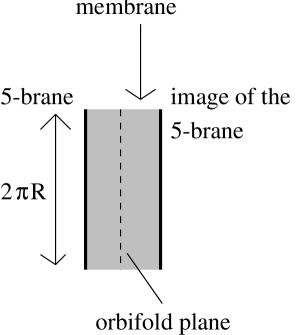
Figure 13: Membrane stretched between the M5-brane and its image under ${\cal I}_{5}\cdot\sigma$. We shall consider the case where the 5-brane (and its image) coincide with the orbifold plane.

The five-brane world-volume carries a self-dual anti-symmetric tensor field $B_{MN}$. The component $B_{1\mu}$, where $x^{1}$ denotes the coordinate along $S^{1}$ and $\mu$ is the coordinate along $R^{4,1}$, is the SO(2) gauge field $A_{\mu}$ on the D4-O4 system. As displayed in Fig.13, the world-volume of the five brane placed at the origin of $R^{5}$ also contains a non-BPS string from the membrane stretched between the five-brane and its image under ${\cal I}_{5}\cdot\sigma$[1]. Although we cannot explicitly compute the tension of this string, by dimensional analysis we see that this tension must be proportional to $m_{p}^{2}$, since this is the only scale in the problem.

Since the non-BPS string carries $B_{MN}$ charge, this string wrapped on $S^{1}$ will be electrically charged under $B_{1\mu}=A_{\mu}$. The mass of this state is given by:

$$C_{4}m_{p}^{2}R=C_{4}m_{S}(g_{S})^{1\over 3}\,,$$ (5.12)

where $C_{4}$ is an unknown numerical constant. On the other hand, the non-BPS string with world-volume along $R^{4,1}$ will be magnetically charged under the gauge field $B_{1\mu}=A_{\mu}$, and its tension will be given by:

$$(\widetilde{C}_{4})^{2}m_{p}^{2}=(\widetilde{C}_{4})^{2}(m_{S})^{2}(g_{S})^{-{2\over 3}}\,,$$ (5.13)

where $\widetilde{C}_{4}$ is a numerical constant related to $C_{4}$. Eqs.(5.12) and (5.13) reproduce the third rows of tables 1 and 2 respectively.

$p=3$

The system under study is the D3-brane on top of an O3-plane in type IIB string theory. The strong coupling limit of this system is dual to a weakly coupled type IIB string theory in the same background, with the parameters of the dual theory related to those in the original theory by eq.(5.9). The electrically charged state in the original theory is mapped to the magnetically charged state in the dual theory. Unfortunately at present we do not know anything about this state, as was discussed earlier in subsection 5.1. On the other hand, the magnetically charged state in the original theory is mapped to the electrically charged state in the dual theory. This is a perturbative open string state, and has mass proportional to $\widetilde{m}_{S}$ for small $\widetilde{g}_{S}$. Thus the mass of the magnetically charged state in the original theory in the strong coupling limit is give by:

$$\widetilde{C}_{3}\widetilde{m}_{S}=\widetilde{C}_{3}m_{S}(g_{S})^{-{1\over 2}}\,,$$ (5.14)

where $\widetilde{C}_{3}$ is a known numerical constant. This reproduces the last row of table 2.

5.3 Electrostatic self-energy of the electrically charged non-BPS particle on the D3-brane $-$ O3-plane system

In this subsection we shall give a lower bound on the electrostatic self-energy of the electrically charged non-BPS particle on the D3-brane $-$ O3-plane system in the strong coupling limit. To do this we go to the dual weakly coupled description where this particle corresponds to a magnetically charged particle on the D3-brane $-$ O3-plane world-volume. Although we do not know at present how to explicitly construct this state, it is clear that sufficiently far away from the center, the magnetic field around the state will look like the magnetic field of a point monopole. Let $r_{c}$ be the distance beyond which this happens. If we normalize the gauge field on the D3-brane so that the action has the form:

$${1\over\widetilde{g}_{S}}\int d^{4}xF_{\mu\nu}F^{\mu\nu}\,,$$ (5.15)

where $\widetilde{g}_{S}$ as usual is the string coupling constant in this dual string theory, then the magnetic field for $r>>r_{c}$ is of order $(1/r^{2})$, and hence its contribution to the total energy of the system from the region $r\geq r_{c}$ is of order

$${1\over\widetilde{g}_{S}}\int_{r\geq r_{c}}{d^{3}r\over r^{4}}\sim(\widetilde{g}_{S})^{-1}(r_{c})^{-1}\,.$$ (5.16)

In order to give a lower bound to this expression we need an upper bound on $r_{c}$. This is obtained by noting that $r_{c}$ cannot be larger than the string scale $(\widetilde{m}_{S})^{-1}$ in this dual string theory, since for small $\widetilde{g}_{S}$ we expect the lightest massive states in this theory to have mass of order $\widetilde{m}_{S}$. Thus beyond the distance $(\widetilde{m}_{S})^{-1}$, the magnetic field of the monopole should approach that of a point monopole. This gives the following lower bound to the magnetostatic energy:

$$\widetilde{m}_{S}(\widetilde{g}_{S})^{-1}\sim m_{S}(g_{S})^{1\over 2}\,.$$ (5.17)

This exceeds the expected answer $m_{S}(g_{S})^{1\over 4}$ from eq.(5.2).

This suggests that eq.(5.2) is applicable, if at all, only to the ‘intrinsic mass’ of the non-BPS particle (if it could be defined at all), and cannot account for the contribution from the Coulomb energy. Presumably the issue will be clarified once we have an explicit construction of this non-BPS state. It is the same problem which appears in a more severe form in the case of $p=2$. Here the electrostatic self-energy is infinite, and completely masks the ‘intrinsic mass’ of the particle.

6 Some Related Developments

In this section we shall briefly discuss some other related developments in this field. In particular, we shall discuss

1. construction of other non-BPS states in type I string theory[7],

2. relationship between D-brane charge and K-theory[7, 9], and

3. application of boundary state formalism to the study of non-BPS states[4].

There are several other related developments[45, 46, 47, 48, 49, 50, 51, 52] which will not be discussed here. At the end we shall also briefly discuss some open problems.

6.1 Other non-BPS branes in type I string theory

In the same way that we constructed a D0-brane in type I string theory, one can construct a D8-brane in this theory. The idea is to start with the non-BPS D8-brane of type IIB string theory, and mod it out by the world-sheet parity transformation $\Omega$. The result is a non-BPS D8-brane of type I string theory. The tachyonic mode of the open string with both ends on the 8-brane is projected out as in the case of the D0-brane. However in type I string theory there are also space filling D9-branes, and it turns out that open strings with one end on the D8-brane and the other end on a D9-brane has tachyonic modes which are not projected out[53]. Thus these branes are not stable.

One can also construct non-BPS D-instantons in the type I string theory as follows[7]. We can start from a D-instanton anti-D-instanton pair of type IIB string theory, and mod out the theory by the world-sheet parity transformation $\Omega$. The result is a non-BPS D-instanton of type I string theory. One can show that the tachyonic mode is projected out under this operation; so that the D-instanton is a stable configuration of type I string theory.

A similar construction can be done by starting with a D7-brane $-$ ${\bar{\rm D}}$7-brane pair of type IIB string theory, and modding out the configuration by $\Omega$. Again the tachyonic mode originating in open strings with both ends on the D7-brane is projected out. But in this case there is a tachyonic mode in the open strings with one end on the D7-brane and the other end on the D9-brane. Thus the D7-brane is not a stable configuration in type I string theory[53].

6.2 K-theory

Another related development in this field has been the discovery of the relationship between elements of the K-group of space-time manifold and D-brane charges on the same manifold[7]. This is related to the idea of representing a D-brane as a tachyonic soliton on a D-brane - anti-D-brane pair of higher dimensions. The simplest example is that of type IIB string theory, so we shall only discuss this case. In this case, following the discussions of section 4 we see that a BPS D-$(2p+1)$-brane can be regarded as a soliton solution on a D-$(2p+3)$ $-$ ${\bar{\rm D}}$-$(2p+3)$-brane pair. Each of the D-$(2p+3)$ branes on the other hand can be regarded as a soliton solution on a D-$(2p+5)$-brane ${\bar{\rm D}}$-$(2p+5)$-brane pair. Following this argument we see that each stable D-brane in type IIB string theory can be regarded as some kind of soliton solution on a sufficient number ($N$) of 9-brane $-$ anti-9-brane pair. It was shown by Witten[7] that the solution representing a system of D-branes (possibly with some gauge field configurations on them) can be completely classified by specifying the $U(N)$ gauge bundles $E$ and $F$ on the 9-brane and the anti-9-brane which characterize the gauge field configurations corresponding to this soliton. Furthermore, if we add equal number of extra 9-branes and anti-9-branes to the system with identical gauge bundles $H$ on them, then the tachyon associated with the open strings stretched between the 9-brane and the anti-9-brane is a section of a trivial bundle, and hence can condense to the minimum ($T_{0}$) of the potential everywhere on the 9-brane $-$ anti-9-brane world-volume. Since this configuration is identical to the vacuum, we conclude that adding such extra pairs of 9-brane and anti-9-brane has no effect on the topological class of the soliton. Thus the D-brane charges are classified by specifying a pair of U(N) vector bundles $(E,F)$ subject to the equivalence relation

$$(E,F)\equiv(E+H,F+H)\,,$$ (6.1)

for any U(M) vector bundle $H$. This is precisely the definition of the K-group of the space-time manifold.

This is the basic idea of using K-theory to classify D-brane charges. Similar analysis can be carried out for type I and type IIA string theories as well. In type I theory the starting point is the representation of all D-branes as solitons on D9-${\bar{\rm D}}$9-brane system[7], whereas in type IIA string theory the starting point is the representation of a D-brane as a soliton on a system of non-BPS D9-branes[9].

6.3 Boundary state approach to non-BPS branes

The boundary state approach[54, 55, 56, 57, 61] to the study of non-BPS D-branes was pioneered by Bergman and Gaberdiel[4]. Corresponding to any D-brane in string theory, we can associate a boundary state $|B\rangle$ in the closed string sector whose inner product with a closed string state describes the amplitude for a closed string emission from the D-brane. Furthermore, if $|B\rangle$ and $|B^{\prime}\rangle$ denote the boundary states associated with a pair of (not necessarily identical) D-branes, then $\langle B|B^{\prime}\rangle$ describes the one loop partition function of an open string stretched from the first D-brane to the second D-brane. The boundary state $|B_{p}\rangle$ of a BPS D-$p$-brane in type IIA or type IIB string theory can be written as a sum of two terms:

$$|B_{p}\rangle={1\over\sqrt{2}}(|NSNS_{p}\rangle+|RR_{p}\rangle)\,,$$ (6.2)

where $|NSNS_{p}\rangle$ and $|RR_{p}\rangle$ denote the contribution to the boundary state from the NSNS and RR sector closed strings respectively. The inner product $\langle B_{p}|B_{q}\rangle$ can be expressed as

$$\langle B_{p}|B_{q}\rangle=Tr_{p-q}{1+(-1)^{F}\over 2}\,,$$ (6.3)

where $Tr_{p-q}$ denotes trace over the open string states stretched from the D-$p$-brane to the D-$q$-brane. In this equation the contribution proportional to 1 comes from the NSNS component of the boundary state, whereas the contribution proportional to $(-1)^{F}$ comes from the RR component of the boundary state.

In this notation the boundary state $|\widetilde{B}_{p}\rangle$ describing the non-BPS D-$p$-brane of type IIB or type IIA string theory is given by[4, 6]

$$|\widetilde{B}_{p}\rangle=|NSNS_{p}\rangle\,.$$ (6.4)

Note that the contribution from the RR sector is absent, reflecting the fact that the non-BPS D-brane does not carry any RR charge. Also the NSNS sector contribution to (6.4) has an extra factor of $\sqrt{2}$ compared to that in (6.2). This reflects the fact that the non-BPS D-brane has an extra multiplicative factor of $\sqrt{2}$ in its tension.

From eqs.(6.2)-(6.4) it follows that

$$\langle\widetilde{B}_{p}|\widetilde{B}_{p}\rangle=Tr_{p-p}(1)\,.$$ (6.5)

This shows that the partition function of open string states living on the non-BPS D-brane has no GSO projection.

One can also analyse the fate of stable non-BPS D-branes in various orbifolds and orientifolds of type II string theories using the boundary state approach. Let us consider, for example, the case of type I D-particle. In this case the boundary state is described by

$${1\over\sqrt{2}}(|\widetilde{B}_{0}\rangle+32|B_{9}\rangle+|C\rangle)\,,$$ (6.6)

where $|\widetilde{B}_{0}\rangle$ is the boundary state of the non-BPS D0-brane (the $(1/\sqrt{2})$ factor is due to the $\Omega$ projection), $32|B_{9}\rangle$ denotes the boundary state corresponding to the 32 BPS D9-branes in the vacuum, and $|C\rangle$ is the crosscap state[54, 55, 56, 57] reflecting the effect of $\Omega$ projection. The terms involving $|\widetilde{B}_{0}\rangle$ in the inner product of this boundary state with itself is given by

$${1\over 2}(\langle\widetilde{B}_{0}|\widetilde{B}_{0}\rangle+\langle\widetilde{B}_{0}|C\rangle+\langle C|\widetilde{B}_{0}\rangle+32\langle\widetilde{B}_{0}|\widetilde{B}_{9}\rangle+32\langle\widetilde{B}_{9}|\widetilde{B}_{0}\rangle)\,.$$ (6.7)

The sum of the first three terms gives

$$Tr_{0-0}{1+\Omega\over 2}\,,$$ (6.8)

where $Tr_{0-0}$ denotes trace over open strings with both ends on the D0-brane. On the other hand the last two terms give

$$32Tr_{0-9}(1)\,,$$ (6.9)

where $Tr_{0-9}$ denotes the trace over open string states stretched from the D0-brane to the D9-brane. There is no $\Omega$ projection in this term, since $\Omega$ relates these open strings to open strings stretched from the D9-brane to the D0-brane. Thus the effect of $\Omega$ projection is to simply include either the $0-9$ or the $9-0$ sector, but not both.

Since $|\widetilde{B}_{0}\rangle$, $|C\rangle$ and $|B_{9}\rangle$ are all explicitly known, we can evaluate each term in (6.7) explicitly. Comparing these with (6.8) we can explicitly derive the $\Omega$ projection rules for the open strings with both ends on the non-BPS D0-brane, and check that these rules agree with the ones derived following the arguments in subsection 3.1. In particular, one can verify that the tachyonic mode on this D-particle is projected out under $\Omega$.

6.4 Open questions and speculations

We shall conclude this article by reviewing some of the open questions and with some speculations.

1. The various arguments given in favour of the idea that the tachyonic ground state on the brane anti-brane pair is indistinguishible from the vacuum are all indirect, and involves first compactifying one or more directions tangential to the brane world-volume, followed by switching on the tachyon vev and then taking the radius back to infinity. A direct proof of this on a non-compact brane-antibrane pair, presumably based on the construction of an explicit classical solution in the open string field theory on the brane-antibrane pair describing the tachyonic ground state, is still lacking. Similarly, one should be able to construct an explicit classical solution in this open string field theory representing the tachyonic kink solution and show that this solution describes a non-BPS D-brane.

2. One of the difficulties in understanding the phenomenon of tachyon condensation on the brane-antibrane pair has been in understanding what happens to the various U(1) gauge fields living on the original system. The tachyon is charged under one combination of the two U(1) gauge fields, and hence breaks this gauge symmetry. However the other linear combination, which we shall denote by ${\cal A}_{\mu}$, does not get broken since the tachyon, as well as all other perturbative open string states living on the brane-antibrane world-volume, are neutral under this gauge field.

   It has been suggested in ref.[45] that the other U(1) is in the confining phase. The suggested mechanism for this confinement is the condensation of the tachyonic $(p-3)$-branes obtained from D-$(p-2)$-branes stretched between the original D-$p$-brane and the anti-D-$p$-brane. Thus for example for $p=3$, it involves condensation of the tachyonic mode of the D-string stretched between the D3-brane and the ${\bar{\rm D}}$3-brane. It was shown in [45] that this tachyon is magnetically charged under ${\cal A}_{\mu}$, and hence condensation of this tachyon will imply that the corresponding U(1) gauge theory is in the confining phase.

   Whereas the general idea is quite appealing, this mechanism is highly non-perturbative from the point of view of the world-volume theory of the D3-brane $-$ ${\bar{\rm D}}$3-brane pair. On the other hand the indirect arguments reviewed in this article showing that the tachyonic ground state is identical to the vacuum configuration are based on open string tree level analysis. Thus there must be a way to see the phenomenon of confinement of the U(1) gauge field ${\cal A}_{\mu}$ at open string tree level. Presumably once we understand how to describe tachyon condensation using classical open string field theory, this issue will be automatically resolved.

3. Another open problem, which has already been discussed earlier, is the construction of magnetically charged non-BPS D-$(p-3)$-brane on the D-$p$-brane $-$ O-$p$-plane system. It is clear that these stable branes must exist in the spectrum, so one should be able to find them in the weakly coupled string theory.

4. It would be interesting to investigate the relationship between weak coupling perturbation expansion for the mass of a non-BPS state and its strong coupling limit. This might give us new insight into string theory at finite coupling.

5. One of the main lessons from our analysis (and of refs.[58, 59, 60]) is that the existence of tachyons in the spectrum of open string theory does not necessarily signify a sickness of the theory, but often simply indicates the existence of a ground state with energy (density) lower than that of the starting configuration. It would be interesting to investigate if closed string tachyons have a similar interpretation.

6. From our discussion in this article it is clear that all D-branes in type IIA (IIB) string theory can be regarded as classical solutions in the open string field theory living on a system of non-BPS D9-branes (D9-brane $-$ ${\bar{\rm D}}$9-brane pair). It would be interesting to see if this can also be done for other known objects in string theory, namely the fundamental string and the NS 5-branes. Actually fundamental strings appear as bound state poles in the S-matrix computed from Witten’s open string field theory[62, 63, 64]. On the other hand a formal construction was presented in [64] showing that any string background represented by a two dimensional conformal field theory (of which the NS five-brane is an example) can be represented as a classical solution in the purely cubic open string field theory. If these results can be made more concrete, then one could take open string field theory on the non-BPS D9-brane (D9-${\bar{\rm D}}$9 brane pairs) as the fundamental formulation of type II string theories and their orbifolds/orientifolds, since all states in string theory could be constructed from this field theory.

Acknowledgement: I would like to thank O. Bergman, S. Elitzur, M. Gaberdiel, P. Horava, N. Manton, B. Pioline, E. Rabinovici, A. Recknagel, V. Schomerus and E. Witten for useful correspondence at various stages of this work. I would also like to thank the organisers of the APCTP winter school for organising an excellent school, and the Tata Institute at Mumbai, IAS at the Hebrew University and CTP at MIT for their hospitality during the preparation of this manuscript.

Appendix A Conformal Field Theory of the Tachyonic Kink Solution

From our discussion in sections 2 and 4, it follows that a non-BPS D-$2p$-brane of type IIB string theory has two descriptions:

• D-$2p-{\bar{\rm D}}$-$2p$ of type IIA string theory modded out by $(-1)^{F_{L}}$, and

• tachyonic kink on D-$(2p+1)-{\bar{\rm D}}$-$(2p+1)$ system of type IIB string theory.

In this appendix we shall address the issue of proving the equivalence of these two descriptions. We shall focus on the non-BPS D0-brane of IIB, but extension to the general case (non-BPS D-$2p$-brane of IIB and non-BPS D-$(2p+1)$-brane of IIA) is straightforward. The details of the analysis of this appendix can be found in ref.[5]. Some related analysis for bosonic string theory can be found in refs.[65, 66, 67, 69, 68].

The outline of the proof is as follows. We begin with the observation that the tachyonic kink on the D1$-{\bar{\rm D}}$1 pair is a classical solution in the open string field theory living on the D1$-{\bar{\rm D}}$1 pair. Thus this configuration must be describable by a two dimensional boundary conformal field theory. Hence we need to

• find this CFT, and

• show that this is equivalent to the CFT describing ${\rm D}0-{\bar{\rm D}}0\hbox{ of IIA}/(-1)^{F_{L}}$.

The next question is: how do we find the CFT describing the kink? This is done using the following steps.

• Find a series of marginal deformations which connect the D1$-{\bar{\rm D}}$1 pair to the tachyonic kink.

• Follow what happens to the CFT describing the D1$-{\bar{\rm D}}$1 pair under this marginal deformation.

Thus our first job will be to find this series of marginal deformations. This is done in several steps.

1. Compactify one direction along a circle $S^{1}$ of radius $R$ and take the D1-${\bar{\rm D}}$1 pair to lie along $S^{1}$. Let $x$ be the coordinate along $S^{1}$, and $A_{\mu}$, $\bar{A}_{\mu}$ be the U(1) gauge fields on D1, ${\bar{\rm D}}$1-branes respectively. The first step is to increase $\bar{A}_{x}$ from 0 to $1/2R$. This is a marginal deformation using boundary operators, and gives

   $$\exp(i\ointop\bar{A}_{x}dx)=-1\,.$$ (A.1)

   In the presence of such a Wilson line, open strings with CP factors $I$ and $\sigma_{3}$ are periodic under $x\to x+2\pi R$, since they are neutral under $\bar{A}_{x}$, whereas open strings with CP factors $\sigma_{1}$ and $\sigma_{2}$ are anti-periodic under $x\to x+2\pi R$ since they carry unit charge under $\bar{A}_{x}$.

2. Let $T$ denote the tachyon field originating in the sector $\sigma_{1}$. This has a Fourier expansion of the form:

   $$T(x,t)=\sum_{n\in Z}T_{n+{1\over 2}}(t)e^{i(n+{1\over 2}){x\over R}}\,,$$ (A.2)

   since it is anti-periodic under $x\to x+2\pi R$. The mass of the mode $T_{n+{1\over 2}}$ is given by

   $$m^{2}_{n+{1\over 2}}={(n+{1\over 2})^{2}\over R^{2}}-{1\over 2}\,.$$ (A.3)

   We now note that

   • For $R\leq(1/\sqrt{2})$ there are no tachyonic modes.

   • For $R=1/\sqrt{2}$, $T_{\pm{1\over 2}}$ is massless and hence represent marginal boundary operators in the CFT.

   In this second step we reduce $R$ from its initial value down to $1/\sqrt{2}$. This corresponds to a marginal deformation involving bulk operators.

3. As we shall see later, at $R={1\over\sqrt{2}}$, $(T_{1\over 2}-T_{-{1\over 2}})$ corresponds to an exactly marginal operator. In this third step we switch on vacuum expectation value (vev) of $(T_{1\over 2}-T_{-{1\over 2}})$. This is a marginal deformation involving a boundary operator.

   

   Figure 14: Effect of switching on vacuum expectation value of $(T_{1\over 2}-T_{-{1\over 2}})$.

   The physical interpretation of switching on the vev of $(T_{1\over 2}-T_{-{1\over 2}})$ is as follows. If we take:

   $$(T_{1\over 2}-T_{-{1\over 2}})=-i\alpha,\qquad T_{1\over 2}+T_{-{1\over 2}}=0,\qquad T_{n}=0\quad\hbox{for}\quad|n|>{1\over 2},\,,$$ (A.4)

   then

   $$T(x)=\alpha\sin{x\over 2R}\,.$$ (A.5)

   As shown in Fig.14, this represents a kink.

   Note that we have not said so far how much vev we should give to $(T_{1\over 2}-T_{-{1\over 2}})$. This will be discussed shortly.

4. After switching on the tachyon vev, we take the radius back to infinity. This corresponds to marginal deformation by a bulk operator.

   

   Figure 15: The flow in the $R-\alpha$ plane from $(R=\infty,\alpha=0)$ to $(R=\infty,\alpha=1)$.

   It will be shown later that when we switch on this marginal deformation, for $R>{1\over\sqrt{2}}$, $(T_{1\over 2}-T_{-{1\over 2}})$ develops a tadpole for a generic $\alpha$. This is not surprising, since for $R>{1\over\sqrt{2}}$, $(T_{1\over 2}-T_{-{1\over 2}})=\alpha$ is not expected to be a solution of the equations of motion for arbitrary $\alpha$. However, we find that there are two values of $\alpha$ for which the tadpole vanishes: namely $\alpha=0$ and $\alpha=1$ (with a suitable normalization of the tachyon field). If we take the limit $R\to\infty$ at $\alpha=0$, we get back the D1-${\bar{\rm D}}$1 pair. But if we take the $R\to\infty$ limit at $\alpha=1$, we should expect to get the kink on the D1-${\bar{\rm D}}$1 pair.

   This analysis also determines the amount of vev of $(T_{1\over 2}-T_{-{1\over 2}})$ to be switched on at the third step. Namely, it should correspond to $\alpha=1$.

The steps 2, 3 and 4 correspond to the flow in the $(R,\alpha)$ plane as shown in Fig.15. Note that if we want to go from the $(R=\infty,\alpha=0)$ point to the $(R=\infty,\alpha=1)$ point directly, we need to perturb by $(T_{1\over 2}-T_{-{1\over 2}})$ at $R=\infty$, which is a relevant boundary operator.

We now carry out these steps in detail and see what conformal field theory we get at the end of these steps. Since marginal deformations up to the end of step 2 is straightforward, we focus on steps 3 and 4. Thus our starting point will be the CFT at the end of step 2. This corresponds to

$$R={1\over\sqrt{2}},\quad\exp(i\ointop\bar{A}_{x}dx)=-1,\quad\alpha=0\,.$$ (A.6)

The relevant world-sheet fields are a scalar field $X\equiv(X_{L}+X_{R})$ representing the coordinate along $S^{1}$, and a Majorana fermion $(\psi_{L},\psi_{R})$ representing the world-sheet supersymmetric partner of $X$. We impose Neumann boundary condition on $X$ and $\psi$:

$$X_{L}=X_{R}\equiv X_{B}/2,\qquad\psi_{L}=\psi_{R}\equiv\psi_{B}\,,$$ (A.7)

where the subscript $B$ stands for boundary value. Besides these fields, there are nine other bosonic coordinate fields, their fermionic partners, and ghost fields, but these will not play any crucial role in our analysis.

Let us now define $h$ to be the transformation $X\to X+2\pi R$. The $h$ and $(-1)^{F}$ quantum numbers of the open string states carrying different CP factors are then given as in table 3.

CP factor	$h$	$(-1)^{F}$
$I$, $\sigma_{3}$	1	1
$\sigma_{1}$, $\sigma_{2}$	-1	-1

Table 3: The $(-1)^{F}$ and $h$ quantum numbers of various open string states at the end of step 2.

Using these rules we can determine the complete spectrum of open strings. In particular vertex operator for $(T_{1/2}-T_{-(1/2)})$ in the 0-picture[70] is given by:

$$V_{T}\sim\psi_{B}(e^{iX_{B}/\sqrt{2}}+e^{-iX_{B}/\sqrt{2}})\otimes\sigma_{1}\,.$$ (A.8)

This is odd under $h$ and $(-1)^{F}$.

We now use the fact that at $R=(1/\sqrt{2})$, a free boson $X$ is equivalent to a pair of Majorana fermions $(\xi,\eta)$. The relationship is of the form:

$$e^{i\sqrt{2}X_{L}}\sim(\xi_{L}+i\eta_{L}),\qquad e^{i\sqrt{2}X_{R}}\sim(\xi_{R}+i\eta_{R})\,.$$ (A.9)

Thus we have three Majorana fermions $\xi$, $\eta$, and $\psi$. We can now rebosonize them as follows:

$$e^{i\sqrt{2}\phi_{L\atop R}}\sim(\xi_{L\atop R}+i\psi_{L\atop R})\,,$$ (A.10)

or

$$e^{i\sqrt{2}\phi^{\prime}_{L\atop R}}\sim(\eta_{L\atop R}+i\psi_{L\atop R})\,.$$ (A.11)

$\phi$ and $\phi^{\prime}$ are scalar fields. The relationship between the currents in the bosonic and the fermionic variables are as follows:

$$\xi_{L}\eta_{L}\sim\partial X_{L},\qquad\xi_{L}\psi_{L}\sim\partial\phi_{L},\qquad\eta_{L}\psi_{L}\sim\partial\phi^{\prime}_{L}\,,$$

$$\xi_{R}\eta_{R}\sim\partial X_{R},\qquad\xi_{R}\psi_{R}\sim\partial\phi_{R},\qquad\eta_{R}\psi_{R}\sim\partial\phi^{\prime}_{R}\,.$$ (A.12)

From eq.(A.7) and (A.9)-(LABEL:ea11) we can easily see that putting Neumann boundary condition on $X$ and $\psi$ corresponds to putting Neumann boundary condition on $\phi,\phi^{\prime},\xi$ and $\eta$:

$$\phi_{L}=\phi_{R}\equiv{1\over 2}\phi_{B},\qquad\phi^{\prime}_{L}=\phi^{\prime}_{R}\equiv{1\over 2}\phi_{B}\,,$$

$$\xi_{L}=\xi_{R}\equiv\xi_{B},\qquad\eta_{L}=\eta_{R}\equiv\eta_{B}\,.$$ (A.13)

We can now rewrite the vertex operator for the tachyon field in terms of the new fields:

$$V_{T} \sim \psi_{B}(e^{iX_{B}/\sqrt{2}}+e^{-iX_{B}/\sqrt{2}})\otimes\sigma_{1}$$ (A.14)

$$\sim \psi_{B}\xi_{B}\otimes\sigma_{1}\sim\partial\phi_{B}\otimes\sigma_{1}\,.$$

Now, $\partial\phi_{B}\otimes\sigma_{1}$ can be interpreted as the vertex operator of a constant gauge field ${\cal A}_{\phi}$ along $\phi$. Hence it corresponds to an exactly marginal deformation, as claimed earlier. Furthermore, ${\cal A}_{\phi}$ is a periodic variable. Let us denote by $\alpha$ a suitably normalized ${\cal A}_{\phi}$ such that $\alpha$ has periodicity 2.

We shall now study the effect of switching on ${\cal A}_{\phi}$ on the open string spectrum. This can be done as follows:

• First of all, since $I$ and $\sigma_{1}$ commute with $\sigma_{1}$, we conclude that open string states with CP factors $I$, $\sigma_{1}$ are neutral under ${\cal A}_{\phi}$. Thus the spectrum in these sectors remain unchanged.

• Since

  $$[\sigma_{1},\sigma_{3}\pm i\sigma_{2}]=\mp 2(\sigma_{3}\pm i\sigma_{2})\,,$$ (A.15)

  we see that open strings in sectors $\sigma_{3}\pm i\sigma_{2}$ carry equal and opposite charges under ${\cal A}_{\phi}$. Thus in these sectors switching on ${\cal A}_{\phi}$ causes a shift in the $\phi$ momentum quantization rule:

  $$p_{\phi}\to p_{\phi}\pm{\alpha\over\sqrt{2}}\,.$$ (A.16)

  The coefficient of $\alpha$ in this equation has been fixed by requiring that $\alpha$ has periodicity 2. From eqs.(A.9)-(A.11) we see that under $(-1)^{F}\cdot h$, $\phi\to\phi+\sqrt{2}\pi$ and $\eta\to-\eta$. Thus projection under $(-1)^{F}\cdot h$ requires that in each CP sector, for fixed set of $\eta$ oscillators, $p_{\phi}$ is quantized as $n\sqrt{2}$ + a constant additive term, where $n$ is an integer. From this we see that shifting $\alpha$ by 2 does not change the quantization law of $p_{\phi}$.

Using these rules we can find the spectrum of open strings for all values of $\alpha$, including at $\alpha=1$. It turns out that the net result for the spectrum at $\alpha=1$ is that in the sectors $(\sigma_{3}\pm i\sigma_{2})$ the GSO projection gets reversed, without any change in the $h$-projection. Thus the $(-1)^{F}$ and $h$ quantum numbers carried by various open string states at $\alpha=1$ are as given in table 4.

CP factor	$h$	$(-1)^{F}$
$I$	1	1
$\sigma_{1}$	-1	-1
$\sigma_{2}$	-1	1
$\sigma_{3}$	1	-1

Table 4. The $(-1)^{F}$ and $h$ quantum numbers of open string states at $\alpha=1$.

Figure 16: Diagram contributing to tachyon one point function to first order in $\delta R$. At the boundary of the disk we must insert a factor of $\exp(i(\alpha/2^{3/2})\sigma_{1}\ointop\partial\phi_{B})$.

This concludes the analysis in step 3. Note that when we combine the spectrum from all the sectors, there is no net $h$ or $(-1)^{F}$ projection, since all combinations of these quantum numbers appear in the spectrum. Thus we can use all combinations of $\xi$, $\eta$ and $\psi$ oscillators to create a state from the Fock vacuum. If we use $\phi^{\prime}$ and $\xi$ as independent variables, then from (A.11) we see that all the states are invariant under $\phi^{\prime}_{L}\to\phi^{\prime}_{L}+\sqrt{2}\pi$, $\phi^{\prime}_{R}\to\phi^{\prime}_{R}+\sqrt{2}\pi$. Since $\phi^{\prime}=\phi^{\prime}_{L}+\phi^{\prime}_{R}$, this effectively corresponds to $\phi^{\prime}$ having a radius $\sqrt{2}$. This fact will be useful to us later.

We now proceed to step 4. This involves switching on the radius deformation and taking the $R\to\infty$ limit. The computation of a correlation function of open string vertex operators on a disk for a generic value of $R$ and $\alpha$ involves

• inserting $\exp({i\alpha\over 2\sqrt{2}}\sigma_{1}\ointop\partial\phi_{B})$ at the boundary, corresponding to the $\alpha$-deformation,

• inserting $\exp(C\int d^{2}z\partial X_{L}\partial X_{R})$ in the interior of the disk corresponding to the radius deformation away from $R={1\over\sqrt{2}}$,

• inserting open string vertex operators corresponding to external states on the boundary, and

• inserting appropriate number of picture changing operators.

As an example we have displayed in Fig.16 the diagram relevant for the computation of tachyon one point function to first order in $\delta R\equiv(R-{1\over\sqrt{2}})$. Here $V_{B}\sim e^{-\Phi_{L}-\Phi_{R}}\psi_{L}\psi_{R}$ is the closed string vertex operator in the $(-1,-1)$ picture representing radius deformation, $(\Phi_{L},\Phi_{R})$ are the left- and the right-moving components of the bosonized ghosts[70], and $V_{T}\sim\partial\phi_{B}\otimes\sigma_{1}$ is the tachyon vertex operator in the $(0,0)$ picture. This diagram can be easily computed, and the final result is that:

$$\langle V_{T}\rangle\propto\sin(\alpha\pi)\,.$$ (A.17)

This vanishes at $\alpha=0,1$. As mentioned earlier, the $\alpha=0$ point corresponds to the original D-string anti-D-string pair, whereas the $\alpha=1$ point corresponds to the tachyonic kink solution on this pair.

Figure 17: Diagrams contributing to the open string tree level amplitude at a general value of $R$ and at $\alpha=1$. The circles denote closed string vertex operators $V_{B}$ corresponding to the radius deformation, and the crosses denote the open string vertex operators corresponding to external open string states. At the boundary of the disk, there is also an insertion of the operator $\exp(i(1/2^{3/2})\sigma_{1}\ointop\partial\phi_{B})$.

We shall from now on focus on the point $\alpha=1$, and analyse the system at a general value of $R$. For general $R$, and a general correlation function of open string vertex operators, we need to sum over all possible number of insertions of $V_{B}=\partial X_{L}\partial X_{R}$, representing the radius deformation in the (0,0) picture, in the interior of the disk with appropriate weight factors. Since we have set $\alpha=1$, we have to insert a factor of

$$\exp\Big{(}i{1\over 2\sqrt{2}}\sigma_{1}\ointop\partial\phi_{B}\Big{)}\,,$$ (A.18)

at the boundary of the disk. The effect of this insertion can be analysed by shrinking the contour integral along the boundary to inside the disk, and picking up the residue at each insertion of $V_{B}$. The final result is that[5] it converts each $\partial X_{L}\partial X_{R}$ to $-\partial\phi^{\prime}_{L}\partial\phi^{\prime}_{R}$. Such a perturbation corresponds to decreasing the $\phi^{\prime}$ radius. Thus we conclude that increasing the $X$ radius at $\alpha=1$ is equivalent to decreasing the $\phi^{\prime}$ radius at $\alpha=0$. In particular, the limit $R_{X}\to\infty$ gets converted to $R_{\phi^{\prime}}\to 0$.

If we introduce a new T-dual variable $\phi^{\prime\prime}$:

$$\phi^{\prime\prime}_{L}=\phi^{\prime}_{L},\qquad\phi^{\prime\prime}_{R}=-\phi^{\prime}_{R},\qquad R_{\phi^{\prime\prime}}=1/R_{\phi^{\prime}}\,,$$ (A.19)

then as $R_{\phi^{\prime}}\to 0$, $R_{\phi^{\prime\prime}}\to\infty$. At the same time, Neumann boundary condition on $\phi^{\prime}$ corresponds to Dirichlet boundary condition on $\phi^{\prime\prime}$

$$\phi^{\prime\prime}_{L}=-\phi^{\prime\prime}_{R}\quad\hbox{at the boundary}\,.$$ (A.20)

The net result is that we have a non-compact bosonic coordinate $\phi^{\prime\prime}$ with Dirichlet boundary condition along $\phi^{\prime\prime}$.

Thus we conclude that the tachyonic kink solution on a D1+${\bar{\rm D}}$1-brane corresponds to a D0-brane at $\phi^{\prime\prime}=0$, where $\phi^{\prime\prime}$ is a new non-compact bosonic coordinate. We can compute the spectrum of open strings with ends on this D0-brane by starting with the known spectrum at the end of step 3 as given in table 4, and following it adiabatically as $R_{\phi^{\prime\prime}}$ increases. We saw that at the end of step 3, the combined spectrum from all sectors has no projection, and $\phi^{\prime}$ behaves like a bosonic coordinate of radius $\sqrt{2}$. Thus $\phi^{\prime\prime}$ has radius $(1/\sqrt{2})$, $-$ the same as that of $X$. As we increase the $X$ radius to some arbitrary value $R$, $\phi^{\prime\prime}$ radius also gets increased to $R$. Thus the combined spectrum of open strings will be that on a D0-brane on a circle of radius $R$, with no GSO projection. This is identical to the one obtained by modding out the D0-${\bar{\rm D}}$0 pair of IIA on a circle of radius $R$ by $(-1)^{F_{L}}$, as studied in section 2.

This shows that a tachyonic kink on the D-string anti-D-string pair of type IIB string theory corresponds to a non-BPS D0-brane of type IIB string theory as defined in section 2. The fact that the non-compact coordinate is called $\phi^{\prime\prime}$ and not $X$ is not of any relevance; all that matters is the CFT describing the system and not how we label the CFT.

As stated at the beginning of this appendix, similar analysis can be done for showing the equivalence of the tachyonic kink on the D-$p-{\bar{\rm D}}$-$p$ pair on IIA (IIB), and $[{\rm D}-(p-1)-{\bar{\rm D}}-(p-1)]/(-1)^{F_{L}}$ in IIB (IIA). Here $p$ is an even integer in type IIA string theory, and is an odd integer in type IIB string theory.

One can also consider a T-dual version of the analysis described here to interpolate between a a D0-brane $-$ ${\bar{\rm D}}0$-brane pair situated at diametrically opposite points on a circle, and a non-BPS D-string wrapped on the same circle. Running the flow backwards, we see that there is a series of marginal deformations which take us from a non-BPS D-string in type IIA string theory to a D0-brane $-$ ${\bar{\rm D}}0$-brane pair in the same theory. By analysing what background corresponds to this deformation on the non-BPS D-string, one discovers that it describes a kink-antikink pair[8]. This allows us to identify a tachyonic kink on the non-BPS D-string to a BPS D-particle of type IIA string theory. This can easily be generalized to show that a tachyonic kink on the non-BPS D-$(p-1)$ brane corresponds to the BPS D-$(p-2)$ brane in the same theory. Again $p$ is even for type IIA string theory and odd for type IIB string theory.

References

- [1] A. Sen, JHEP 06, 007 (1998) hep-th/9803194.
- [2] A. Sen, JHEP 08, 010 (1998) hep-th/9805019.
- [3] A. Sen, JHEP 08, 012 (1998) hep-th/9805170.
- [4] O. Bergman and M.R. Gaberdiel, Phys. Lett. B441, 133 (1998) hep-th/9806155.
- [5] A. Sen, JHEP 09, 023 (1998) hep-th/9808141.
- [6] A. Sen, JHEP 10, 021 (1998) hep-th/9809111.
- [7] E. Witten, JHEP 12, 019 (1998) hep-th/9810188.
- [8] A. Sen, JHEP 12, 021 (1998) hep-th/9812031.
- [9] P. Horava, hep-th/9812135.
- [10] O. Bergman and M.R. Gaberdiel, JHEP 03, 013 (1999) hep-th/9901014.
- [11] H. Garcia-Compean, hep-th/9812226.
- [12] S. Gukov, hep-th/9901042.
- [13] K. Hori, hep-th/9902102.
- [14] E. Sharpe, hep-th/9902116.
- [15] O. Bergman, E.G. Gimon and P. Horava, hep-th/9902160.
- [16] K. Olsen and R.J. Szabo, hep-th/9904153.
-
[17]
J. Dai, R. Leigh, and J. Polchinski, Mod. Phys. Lett.
A4 (1989) 2073;
R. Leigh, Mod. Phys. Lett. A4 (1989) 2767;
J. Polchinski, Phys. Rev. D50 (1994) 6041 [hep-th/9407031];
J. Polchinski, S. Chaudhury and C. Johnson, [hep-th/9602052];
J. Polchinski, [hep-th/9611050]. - [18] M.B. Green, Phys. Lett. B329, 435 (1994) hep-th/9403040.
- [19] T. Banks and L. Susskind, hep-th/9511194.
- [20] M.B. Green and M. Gutperle, Nucl. Phys. B476, 484 (1996) hep-th/9604091.
- [21] G. Lifschytz, Phys. Lett. B388, 720 (1996) hep-th/9604156.
- [22] V. Periwal, hep-th/9612215.
- [23] J.H. Schwarz, Phys. Rept. 89, 223 (1982).
- [24] E. Witten, Nucl. Phys. B443, 85 (1995) hep-th/9503124.
- [25] A. Dabholkar, Phys. Lett. B357, 307 (1995) hep-th/9506160.
- [26] C.M. Hull, Phys. Lett. B357, 545 (1995) hep-th/9506194.
- [27] J. Polchinski and E. Witten, Nucl. Phys. B460, 525 (1996) hep-th/9510169.
- [28] M.R. Douglas and G. Moore, hep-th/9603167.
- [29] K. Becker, M. Becker and A. Strominger, Nucl. Phys. B456 130 (1995) hep-th/9507158.
- [30] P. Aspinwall, Phys. Lett. B357 329 (1995) hep-th/9507012.
-
[31]
A. Sagnotti, ‘Open Strings and their Symmetry Groups’, Talk at
Cargese Summer Inst., 1987;
G. Pradisi and A. Sagnotti, Phys. Lett. B216 59 (1989);
M. Bianchi, G. Pradisi and A. Sagnotti, Nucl. Phys. B376 365 (1992);
P. Horava, Nucl. Phys. B327 461 (1989), Phys. Lett. B231 251 (1989). - [32] E. Gimon and J. Polchinski, Phys. Rev. D54 1667 (1996) [hep-th/9601038].
- [33] E. Witten, JHEP 02, 006 (1998) hep-th/9712028.
- [34] A. Sen, Nucl. Phys. B475, 562 (1996) hep-th/9605150.
- [35] A. Strominger, Phys. Lett. B383, 44 (1996) hep-th/9512059.
- [36] P.K. Townsend, Phys. Lett. B373, 68 (1996) hep-th/9512062.
- [37] M.F. Atiyah and N.J. Hitchin, Phil. Trans. Roy. Soc. Lond. A315, 459 (1985); “The Geometry And Dynamics Of Magnetic Monopoles. M.B. Porter Lectures,” PRINCETON, USA: UNIV. PR. (1988) 133p.
- [38] N. Seiberg and E. Witten, hep-th/9607163.
- [39] G.W. Gibbons and P.J. Ruback, Commun. Math. Phys. 115, 267 (1988).
- [40] N.S. Manton and B.J. Schroers, Ann. Phys. 225, 290 (1993).
- [41] A. Sen, Phys. Lett. B329, 217 (1994) hep-th/9402032.
- [42] A. Sen, Nucl. Phys. B474, 361 (1996) hep-th/9604070.
- [43] K. Dasgupta and S. Mukhi, Nucl. Phys. B465, 399 (1996) hep-th/9512196.
- [44] E. Witten, Nucl. Phys. B463, 383 (1996) hep-th/9512219.
- [45] P. Yi, hep-th/9901159.
- [46] H. Awata, S. Hirano and Y. Hyakutake, hep-th/9902158.
- [47] N. Kim, S. Rey and J. Yee, JHEP 04, 003 (1999) hep-th/9903129.
- [48] M. Gutperle and V. Periwal, JHEP 02, 018 (1999) hep-th/9812003.
- [49] M. Srednicki, JHEP 08, 005 (1998) hep-th/9807138.
- [50] O. Bergman and B. Kol, Nucl. Phys. B536, 149 (1998) hep-th/9804160.
- [51] M.J. Strassler, hep-th/9709081, hep-lat/9803009, hep-th/9808073.
- [52] I. Pesando, “On the effective potential of the Dp - anti-Dp system in type II theories,” hep-th/9902181.
- [53] M. Frau, L. Gallot, A. Lerda and P. Strigazzi, hep-th/9903123.
- [54] J. Polchinski and Y. Cai, Nucl.Phys. B296 91 (1988).
- [55] C. Callan, C. Lovelace, C. Nappi and S. Yost, Nucl.Phys. B308 221 (1988).
- [56] T. Onogi and N. Ishibashi, “Conformal Field Theories On Surfaces With Boundaries And Crosscaps,” Mod. Phys. Lett. A4, 161 (1989).
- [57] N. Ishibashi, “The Boundary And Crosscap States In Conformal Field Theories,” Mod. Phys. Lett. A4, 251 (1989).
- [58] J. Polchinski and A. Strominger, “New vacua for type II string theory,” Phys. Lett. B388, 736 (1996) hep-th/9510227.
- [59] E. Gava, K.S. Narain and M.H. Sarmadi, “On the bound states of p-branes and (p+2)-branes,” Nucl. Phys. B504, 214 (1997) hep-th/9704006.
- [60] I. Antoniadis, E. Gava, K.S. Narain and T.R. Taylor, “Duality in superstring compactifications with magnetic field backgrounds,” Nucl. Phys. B511, 611 (1998) hep-th/9708075.
-
[61]
O. Bergman and M. Gaberdiel, Nucl.Phys. B499 183 (1997)
hep-th/9701137;
M. Li, Nucl.Phys. B460 351 (1996) hep-th/9510161;
H. Ooguri, Y. Oz and Z. Yin, Nucl.Phys. B477 407 (1996) hep-th/9606112;
K. Becker, M.Becker, D. Morrison, H. Ooguri, Y. Oz and Z. Yin, Nucl. Phys. B480 225 (1996) hep-th/9608116;
M. Kato and T. Okada, Nucl. Phys. B499 583 (1997) 583 hep-th/9612148;
S. Stanciu, hep-th/9708166;
A. Recknagel and V. Schomerus, hep-th/9712186;
J. Fuchs and C. Schweigert, hep-th/9712257;
S. Stanciu and A. Tseytlin, hep-th/9805006;
M. Gutperle and Y. Satoh, hep-th/9808080;
F. Hussain, R. Iengo, C. Nunez and C. Scrucca, Phys. Lett. B409 101 (1997) hep-th/9706186;
M. Bertolini, R. Iengo and C. Scrucca, hep-th/9801110;
M. Bertolini, P. Fre, R. Iengo and C. Scrucca, hep-th/9803096;
P. Di Vecchia, M. Frau, A. Lerda, I. Pesando, R. Russo and S. Sciuto, Nucl. Phys. B507 259 (1997) hep-th/9707068;
M. Billo, P. Di Vecchia, M. Frau, A. Lerda, I. Pesando, R. Russo and S. Sciuto, Nucl. Phys. B526 199 (1998) hep-th/9802088; hep-th/9805091. - [62] E. Witten, Nucl. Phys. B268 253 (1986).
- [63] E. Witten, Nucl. Phys. B276 291 (1986).
- [64] A. Strominger, G. T. Horowitz, J. Lykken and R. Rohm, Phys. Rev. Lett. 57 283 (1986).
- [65] C.G. Callan, I.R. Klebanov, A.W. Ludwig and J.M. Maldacena, Nucl. Phys. B422, 417 (1994) hep-th/9402113.
- [66] J. Polchinski and L. Thorlacius, Phys. Rev. D50, 622 (1994) hep-th/9404008.
- [67] A. Recknagel and V. Schomerus, hep-th/9811237.
- [68] S. Elitzur, E. Rabinovici and G. Sarkisian, “On least action D-branes,” Nucl. Phys. B541, 246 (1999) hep-th/9807161.
- [69] A. Sen, hep-th/9902105.
- [70] D. Friedan, E. Martinec and S. Shenker, Nucl. Phys. B271, 93 (1986).