hep-th/9904197 Holography, Thermodynamics and Fluctuations of Charged AdS Black Holes

Abstract

The physical properties of Reissner–Nordström black holes in $(n{+}1)$–dimensional anti–de Sitter spacetime are related, by a holographic map, to the physics of a class of $n$–dimensional field theories coupled to a background global current. Motivated by that fact, and the recent observations of the striking similarity between the thermodynamic phase structure of these black holes (in the canonical ensemble) and that of the van der Waals–Maxwell liquid–gas system, we explore the physics in more detail. We study fluctuations and stability within the equilibrium thermodynamics, examining the specific heats and electrical permittivity of the holes, and consider the analogue of the Clayperon equation at the phase boundaries. Consequently, we refine the phase diagrams in the canonical and grand canonical ensembles. We study the interesting physics in the neighbourhood of the critical point in the canonical ensemble. There is a second order phase transition found there, and that region is characterized by a Landau–Ginzburg model with $A_{3}$ potential. The holographically dual field theories provide the description of the microscopic degrees of freedom which underlie all of the thermodynamics, as can be seen by examining the form of the microscopic fluctuations.

I Introduction and Summary

Explaining the thermodynamic nature of black holes was recognized as an essential hallmark of any complete quantum theory of gravity long before such a theory was constructed. The semi–classical approach to quantum gravity, which has become quite a mature subject over the years[1, 2], allows for the computation of a number of physical quantities. These treatments ignore the details of how a specific solution of Einstein’s equations (regarded as the effective low energy truncation of the complete quantum gravity) arises, and instead perform a quantum treatment of field degrees of freedom in a fixed classical space–time background.

In that way it was learned that the entropy of Bekenstein[3] and the temperature of Hawking[4], for example, fit into an elegant thermodynamic framework, with questions (such as scattering, unitarity, etc.,) concerning the underlying microscopic description —which we might use to construct the underlying “Statistical Mechanics”— best left for the future development of a quantum theory of gravity.

That future is now here. String theory (and/or “M–theory”) supplies a microscopic description of the underlying degrees of freedom upon which a statistical description of the laws of black hole thermodynamics can be based. This is true even though we do not yet have a satisfactory way of writing the theory in all regimes: the “D–brane calculus” [5] provides a robust framework within which to describe many properties of black holes[6], while in turn being firmly rooted in the dynamical framework of string duality and, ultimately, M–theory[7]. Typically, the description of black holes (and other important geometrical backgrounds) proceeds by translating their properties into properties of an auxiliary field theory, identified as residing on the world–volume of some collection of (D– or M–) branes.

One of the succinct ways of organizing this microscopic description of the properties of black holes is via “AdS Holography”[8, 9, 10, 11, 12]. Then, the thermodynamic properties of black holes in anti–de Sitter space–time are dual to those of a field theory in one dimension fewer[10, 11]. The fact that the thermodynamic properties of the AdS black holes[13] are organized by an effective field theory is not implausible, in the light of the fact that AdS acts like a natural “box” (with reflecting walls) which neutralizes the tendency of gravitational interactions to render a canonical thermodynamic ensemble unstable. The fact that the effective field theory is one which does not contain gravity, and that it is actually a “holographically” dual four dimensional gauge theory (with suitable generalizations beyond $D{=}4$) is another striking example of the fundamental role that gauge theory plays in duality in various situations.

That the AdS arena stabilizes the thermodynamics of black holes is especially apparent when one discovers phase structures completely analogous to familiar thermodynamic systems from elsewhere in Nature. Such an example can be found in the Reissner–Nordstrom–anti–de–Sitter (RNadS) systems in various dimensions[17]. There, the $(Q,T)$ diagram showing the thermally stable phases for a fixed charge (canonical) ensemble turns out to be completely analogous to that of the $(T,P)$ phase diagram of the liquid–gas system. The structure of the first order phase transitions, etc., are controlled by a “cusp” catastrophe[18], common in the theory of discontinuous transitions in thermodynamics and many other fields. Meanwhile the free energy as a function of temperature $F(T)$, displays the characteristic “swallowtail” shape.

In this paper, we report the results of our further examination of these structures, exploring the equilibrium thermodynamics more closely, including the effects of considering electrical stability, and thermal fluctuations. The similarities noted between the RNadS physics and that of well–defined systems such as the liquid–gas are more than mere analogies: We find that everything has a very natural place in classic equilibrium thermodynamics, as is consistent with a holographic duality to thermal field theory without gravity. Accordingly, using the techniques of equilibrium thermodynamics, we refine the phase diagrams which we found in ref.[17] somewhat, and identify the generic physical properties which give rise to the cusp and swallowtail structures.

As discussed in our previous paper [17], the thermodynamics of the Reissner–Nordström black holes in the presence of negative cosmological constant in various dimensions are pertinent (because of the holographic map) to the thermodynamics of families of field theories found on the common world–volume of collections of large numbers of branes (for example M2– and D3–branes), in the situation where a global background current (or its canonical conjugate charge) has been switched on and held fixed.

Geometrically this is performed by simply setting the M2– and D3–branes rotating equally in each of the available transverse orthogonal two–planes. The higher dimensional angular momentum becomes the Maxwell $U(1)$ charge after the Kaluza–Klein reduction on the (now twisted) sphere, which yields the gauged supergravity. Obtaining a pure Maxwell term in this way is not possible starting with the M5–brane, and so the seven dimensional Einstein–Maxwell–anti–de–Sitter (EMadS₇) theory defines at best a close cousin to the field theory found on the M5–branes’ world–volumes. The dual theory relevant to EMadS₆ should be considered in a similar manner.

A truly rich phase structure for the field theories (with transition temperatures away from $T{=}0$) is obtained only for finite volume, which is the case we concentrate on here. Our studies correspond to the study of black holes with spherical horizons, $S^{n-1}$. The field theory resides on ${\hbox{{\rm I}\kern-1.99997pt\hbox{\rm R}}}{\times}S^{n-1}$. The case of infinite volume corresponds to black holes with horizons ${\hbox{{\rm I}\kern-1.99997pt\hbox{\rm R}}}^{n-1}$, and to field theory on ${\hbox{{\rm I}\kern-1.99997pt\hbox{\rm R}}}^{n}$. This is of course the case which comes from taking directly the near horizon limit of explicit brane solutions.

As shown in ref.[17], the results for infinite volume may be easily obtained as a scaling limit of the results of finite volume, and so we will not discuss them here. Of course, even though we are in finite volume for much of our discussion, the thermodynamic limit is still valid here, because the dual field theory is at large $N$, and a positive power of $N$ measures the number of degrees of freedom in the field theory (for example, $N^{2}$ in the case of gauge theory, for $n{=}4$ here).

The structure of the paper is as follows: In section II we recall the charged black solutions of the Einstein–Maxwell–anti–de–Sitter system. We also recall the results of performing the Euclidean section and ensuring its regularity. In section III, we translate these results into a statement of about the relation between the thermodynamic variables of the black hole system in thermodynamic equilibrium i.e., the “equation of state”. In section IV, we define the grand canonical and canonical thermodynamic ensembles and compute the associated Gibbs and Helmholtz thermodynamic potentials, contrasting the techniques used (and results obtained) to those of our previous work. In particular, we note that we can obtain an intrinsic definition of these quantities in Euclidean quantum gravity, by sidestepping some of the technical subtleties —encountered in the “background subtraction” technique for regularizing the action— in favour of the “counterterm subtraction” technique[21, 22]. In the rest of the section, we examine the features of these potentials quite closely, in preparation for later detailed studies. In section V, we use the equation of state and the first law of thermodynamics to identify the origins of the crucial features of the shape of the Helmholtz potential (free energy). This “swallowtail” shape is responsible for the interesting phase structure in the canonical ensemble. Section VI examines the conditions for thermodynamic stability of the black holes, examining the specific heats and permittivity of the black holes. In this way, we identify the stable regions of the solution space of the equation of state. We use this stability information, together with the information gained in earlier sections, to deduce the refined phase diagrams exhibited in section VII, and some details of the phase diagrams (the slope and convexity of the coexistence curves) are refined by using the Clayperon equation in section VIII.

As already stressed in this section, the thermodynamic quantities and studies performed in those sections are rooted firmly in a microscopic description. This is ensured by the fact that we can in principle embed this entire discussion into a complete theory of quantum gravity: string (and/or) M–theory. In practical terms, this microscopic description —the “statistical mechanics” underlying the thermodynamics— is summarized neatly in terms of the holographically dual field theory. In this way, therefore we may carry our calculations further and examine the nature and magnitude of the microscopic fluctuations of the various thermodynamic quantities we have computed, knowing that we have a description of their origin in field theory. Thus, we find in section IX that the fluctuations behave in a way consistent with the underlying microscopic physics being supplied by the field theory: the size of the (squared) fluctuations is controlled by a prefactor which corresponds to precisely the inverse of the number of degrees of freedom of the dual field theory. We observe that the size of the fluctuations diverges as the system approaches a critical point in the $(Q,T)$ plane.

Through most of the paper, we carried out our computations for the four dimensional case, in order to keep many of our formulae simple. Section X collects together some of the results for the computation of various quantities. We stress that the qualitative structure of the physics is the same for all dimensions $d{\geq}4$, where $d{=}n{+}1$. Briefly, we also discuss in that same section the issue of the meaning of the formal definition of other thermodynamic ensembles by Legendre transform. It is not always the case that the thermodynamic quantities thus defined may be arrived at by (known) computations in Euclidean quantum gravity. Therefore, interpretations of the physics of such ensembles are to be taken with (at least) a pinch of salt, until such time as new technology becomes available to compute the relevant quantities directly in quantum gravity, as we have done here for the fixed potential (grand canonical) and fixed charge (canonical) ensembles.

Section XI discusses the underlying structure of the phase structure of the canonical ensemble in the neighbourhood of the critical point. In particular, the physics local to critical point is universal for all of dimensions $d{\geq}4$. The critical point is a second order phase transition point at the end of a coexistence line of first order phase transitions. As such, it has a universal description in terms of a Landau–Ginzburg model, with a quartic potential —$A_{3}$ in the $A$–$D$–$E$ classification of such potentials. The deformation of this potential gives the classic “cusp” catastrophe which underlies the critical behaviour, as is well known from the van–der Waals–Maxwell description of the liquid–gas system, with which our black hole physics shares many features, as originally reported in ref. [17].

In closing the introduction, we would like to stress once again how elegantly the properties of anti–de Sitter space yield charged black hole physics so closely akin in structure to that of ordinary field theory–like systems, with which we have more intuition.

From the point of view of the Maxwell part of the action, the black holes are nothing more than spherical capacitors, and as such, the amount of energy they can store grows with the charge on them, but falls with increasing hole radius. From the point of view of the Einstein–Hilbert action however, the black holes store an amount of energy which grows with radius. After a little thought, one might expect on general grounds, therefore, that there might be an interesting phase structure resulting from a competition between these two pieces of the action.

Such reasoning on its own would not be enough to genuinely fill out the whole $(Q,T)$ phase diagram, as the equation of state needs additional structure. It is the presence of (negative) cosmological constant which provides this final part: First, it provides black hole solutions which are thermally stable in ensembles involving fixed temperature[13], but secondly, as it defines a new length scale, is allows the system to distinguish, on the one hand, black holes which are large from those which are small, and on the other hand, black holes which have small charge, from those with large charge.

It is because of these features that the charged black hole thermodynamics has a chance to be similar to the van–der Waals model of the liquid–gas. Recall that without the inclusion of the effects of the length scales set by finite particle size, on the one hand, and attractive inter–particle forces on the other, that system would have only the much less interesting physics of the ideal gas: there would be no competing effects, as a function of length scale, with which to trigger a phase transition. These basic features of AdS give holography a chance to work in a way which is consistent with our intuition that the microscopic physics should be modelled by ordinary field theory.

II Charged AdS Black Holes

For space–time dimension $n{+}1$, the Einstein–Maxwell–anti–deSitter (EMadS_n+1) action may be written as

$$I=-\frac{1}{16{\pi}G}\int_{M}d^{n+1}x\sqrt{-g}\left[R-F^{2}+\frac{n(n-1)}{l^{2}}\right]\ ,$$ (1)

with ${\Lambda}{=}{-}\frac{n(n-1)}{2l^{2}}$ being the cosmological constant associated with the characteristic length scale $l$. Then the metric on the Reissner–Nordström–anti–deSitter (RNadS) solution may be written in static coordinates as[23, 24, 17]

$$ds^{2}=-V(r)dt^{2}+\frac{dr^{2}}{V(r)}+r^{2}d{\Omega}^{2}_{n-1}\ ,$$ (2)

where $d{\Omega}^{2}_{n-1}$ is the metric on the round unit $(n{-}1)$–sphere, and the function $V(r)$ takes the form

$$V(r)=1-\frac{m}{r^{n-2}}+\frac{q^{2}}{r^{2n-4}}+\frac{r^{2}}{l^{2}}\ .$$ (3)

Here, $m$ is related to the ADM mass of the hole, $M$ (appropriately generalized to geometries asymptotic to AdS[25]), as

$$M={(n-1)\omega_{n-1}\over 16\pi G}m\ ,$$ (4)

where $\omega_{n-1}$ is the volume of the unit $(n{-}1)$–sphere. The parameter $q$ yields the charge

$$Q=\sqrt{2(n-1)(n-2)}\left({\omega_{n-1}\over 8\pi G}\right)q\ ,$$ (5)

of the (pure electric) gauge potential, which is

$$A=\left(-{1\over c}{q\over r^{n-2}}+\Phi\right)dt\ ,$$ (6)

where

$$c=\sqrt{2(n-2)\over n-1}\ ,$$ (7)

and $\Phi$ is a constant (to be fixed below). If $r_{+}$ is the largest real positive root of $V(r)$, then in order for this RNadS metric to describe a charged black hole with a non–singular horizon at $r{=}r_{+}$, the latter must satisfy

$$\left({n\over n-2}\right)r_{+}^{2n-2}+l^{2}r_{+}^{2n-4}\geq q^{2}l^{2}\ .$$ (8)

Finally, we choose

$$\Phi={1\over c}{q\over r_{+}^{n-2}}\ ,$$ (9)

which then fixes $A_{t}(r_{+}){=}0$, as is required by (Euclidean) regularity of the one–form potential (6) at the fixed point set of the Killing vector $\partial_{t}$. The physical significance of the quantity $\Phi$, which plays an important role later, is that it is the electrostatic potential difference between the horizon and infinity.

If the inequality in eqn. (8) is saturated, the horizon is degenerate and we get an extremal black hole. This inequality imposes a bound on the black hole mass parameter of the form $m{\geq}m_{e}(q,l)$.

In passing to the thermodynamic discussion, we define the Euclidean section ($t{\to}i\tau$) of the solution, and identify the period, $\beta$, of the imaginary time with the inverse temperature. Using the usual formula for the period, $\beta{=}{4\pi}/{V^{\prime}(r_{+})}$, which arises from the requirement of regularity of the solution, we obtain:

$$\beta=\frac{4{\pi}l^{2}r_{+}^{2n-3}}{nr_{+}^{2n-2}+(n-2)l^{2}r_{+}^{2n-4}-(n-2)q^{2}l^{2}}\ .$$ (10)

This may be rewritten in terms of the potential as:

$$\beta=\frac{4{\pi}l^{2}r_{+}}{(n-2)l^{2}(1-c^{2}\Phi^{2})+nr_{+}^{2}}\ .$$ (11)

For simplicity, we will specialize to $n{=}3$ (therefore working with EMadS₄) to avoid cluttering our expressions with complicated dependences on $n$. Our results will remain qualitatively the same for higher $n$ (see the comments in section XI), and we list some of the $n$–dependent formulae in section X. Our analysis is further simplified by adopting the following rescalings (once we have set $n{=}3$):

$$T\rightarrow{2\pi l\over\sqrt{3}}T\ ,\qquad Q\rightarrow{\sqrt{3}\over l}GQ\ ,\qquad\Phi\rightarrow\Phi$$ (12)

and for the various thermodynamic quantities used in ref.[17],

$$\{W,F,E\}\rightarrow{\sqrt{3}\over l}G\{W,F,E\}\ ,\qquad S\rightarrow{3G\over 2\pi l^{2}}S\ .$$ (13)

$${\rm and}\qquad r_{+}\rightarrow{\sqrt{3}\over l}r_{+}\ .$$ (14)

Essentially we are introducing a system of dimensionless quantities in which everything is measured in units of the AdS scale $l$. This scaling is chosen so that the thermodynamic formulae still all have their standard form, i.e.,

$$dE=TdS+\Phi dQ\ .\qquad dF=-SdT+\Phi dQ\qquad dW=-SdT-Qd\Phi\ ,\ \ {\it etc.}$$ (15)

In the following, all of the quantities which follow are the rescaled dimensionless quantities, unless stated otherwise.

III Equation of State

The Euclidean regularity at the horizon discussed at eqn. (10) is equivalent to the condition that the black hole is in thermodynamical equilibrium. The resulting equation (10) may therefore be written as an equation of state $T{=}T(\Phi,Q)$ (analogous to $T{=}T(P,V)$ for, say, a gas at pressure $P$ and volume $V$). For $n{=}3$, one finds:

$$T={\Phi^{2}(1-\Phi^{2})+Q^{2}\over 2Q\Phi}\ .$$ (16)

One can also solve for $Q$ as

$$Q=T\Phi\pm\Phi\sqrt{T^{2}+\Phi^{2}-1}\ .$$ (17)

From this equation of state we see that for fixed $\Phi$ we get two branches, one for each sign, when the discriminant under the square root is positive. For fixed $Q$, $T(\Phi)$ has three branches for $Q{<}Q_{\rm crit}$ and one for $Q{>}Q_{\rm crit}$, where the critical charge is determined solving for the “point of inflection” where $\left(\partial Q/\partial\Phi\right)_{T}{=}\left(\partial^{2}Q/\partial\Phi^{2}\right)_{T}{=}0.$ In the dimensionless units used here, one finds $Q_{\rm crit}{=}1/(2\sqrt{3})$, $T_{\rm crit}{=}2\sqrt{2}/3$, $\Phi_{\rm crit}{=}1/\sqrt{6}$, $E_{\rm crit}{=}\sqrt{2}/3$, and $r_{\rm+(crit)}{=}1/\sqrt{2}$. It is useful to plot the $(\Phi,Q)$ isotherms, i.e., plot $Q(\Phi)$ for fixed $T$, and we exhibit these in figure 1.

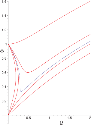
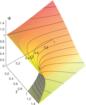
FIG. 1.: Plots of the equation of state of $\Phi$ vs. $Q$, showing isotherms above and below the critical temperature $T_{\rm crit}$. For $T{<}T_{\rm crit}$, there is only one branch of solutions, while for $T{>}T_{\rm crit}$, there are three branches. The values of $T$ for the isotherms plotted are (top down) $T{=}0,0.8,T_{\rm crit},1.0,1.2$. The central (dotted) curve is at the critical temperature.

As $T$ goes to zero, we approach the extremal black holes. Their equation of state is

$$\Phi_{e}^{2}={1\over 2}(1+\sqrt{1+4Q^{2}}),\qquad{\rm for\;arbitrary}\,T.$$ (18)

For some later computations, it is often convenient to use as an additional, non–independent parameter, the black hole radius $r_{+}$, in terms of which

$$Q=r_{+}\sqrt{r_{+}^{2}-2r_{+}T+1},\quad 2T=r_{+}+{1\over r_{+}}-{Q^{2}\over r_{+}^{3}}\ ,$$ (19)

and

$$\Phi={Q\over r_{+}}=\sqrt{r_{+}^{2}-2r_{+}T+1}\ .$$ (20)

IV The grand canonical and canonical ensembles

In thermodynamic parlance, the “grand canonical ensemble” is defined by coupling the system to energy and charge reservoirs at fixed temperature $T$ and potential $\Phi$ (an intensive variable). The associated thermodynamic potential is the Gibbs free energy, $W[T,\Phi]{=}E{-}TS{-}\Phi Q$. Holding the extensive variable, $Q$, fixed, on the other hand, defines the canonical ensemble, with its associated thermodynamic potential is the Helmholtz free energy $F[T,Q]{=}E{-}TS$. See section X for a brief discussion of other ensembles.

In ref. [17], the calculation at fixed potential was carried out by computing the action á la Gibbons–Hawking. With that technique, one must regularize the computation (as the action is formally infinite) by subtracting a contribution from a “reference” background which matches the solution of interest asymptotically, giving a definition of the action relative to that of the reference spacetime. In this case it is appropriate to use AdS —with a fixed (pure gauge) potential at infinity— as the reference background.

Remarkably AdS spacetime provides for another regularization which yields an intrinsic definition of the action. In other words, the computation makes no reference to any other solution of the equations of motion. Instead, the method[21, 22] proceeds by adding a series of boundary counterterms to the action. We refer to this as the “counterterm subtraction” method of defining the action, a technique tailored to spacetimes which are locally asymptotic to anti–de Sitter, as the counterterms are defined on the natural boundary, with which such spaces are endowed, using the AdS scale $l$. Also note that the inclusion of additional sectors to the gravitational and cosmological parts of the action, such as Maxwell terms, does not affect the definitions and therefore we can still use the same counterterms in the present context.

The results, using either the reference background or the counterterm subtraction methods, are identical for the particular case in which we want to fix the potential, since it is possible to have AdS space as a background solution at arbitrary temperature and (constant) potential (but, crucially, see later). In the present notation, the answer is:

$$W[\Phi,T]={1\over 12}\left[3{Q\over\Phi}(1-\Phi^{2})-\left({Q\over\Phi}\right)^{3}\right]\ .$$ (21)

Here, $Q$ is given as $Q(\Phi,T)$ by the equation of state (17). In terms of $r_{+}$, this is

$$W={1\over 12}\left[3r_{+}(1-\Phi^{2})-r_{+}^{3}\right]\ ,$$ (22)

and it is plotted in figure 2, with choice slices displayed in figure 3.

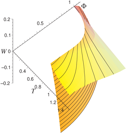
FIG. 2.: Plots of the Gibbs potential $W[\Phi,T]$ in three dimensions.

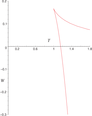
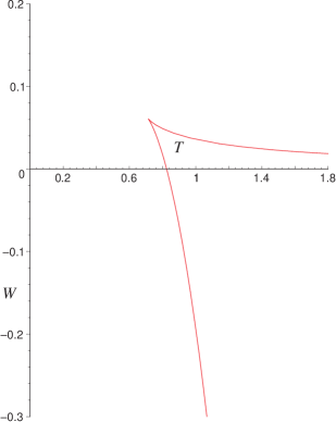
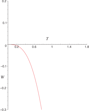
FIG. 3.: Slices of the Gibbs potential $W[\Phi,T]$, for $\Phi{=}0$, $\Phi{=}0.7$ and $\Phi{=}1$.

Turning to the canonical (fixed charge) ensemble, we wish to compute the Helmholtz potential $F[Q,T]$ (a.k.a, the “free energy”). In ref.[17], where we used the reference background method to compute this, it was necessary to compute the action using an extremal black hole as the reference background. This is because anti–de Sitter space with a fixed charge $Q$, as measured at infinity is not a solution of the equations of motion and so is not an appropriate background. In order to get an intrinsic definition of the action for fixed charge therefore, we employ the method of counterterm subtraction, yielding:

$$F[Q,T]={1\over 12}\left[3{Q\over\Phi}-\left({Q\over\Phi}\right)^{3}+9Q\Phi\right]\ ,$$ (23)

where $\Phi$ is given as $\Phi(Q,T)$ by the equation of state (17). In terms of $r_{+}$, $F[Q,T]$ may be written

$$F[Q,T]={1\over 12}\left[3r_{+}-r_{+}^{3}+9{Q^{2}\over r_{+}}\right]\ .$$ (24)

As a consistency check that we have performed the computation correctly, note that this result may be obtained from the result for the Gibbs potential by formally calculating the Legendre transform $F[Q,T]{=}W[\Phi,T]{+}Q\Phi$. When computing $F$ from a Euclidean action, the additional $Q\Phi$ term has its origin in the boundary term introduced so as to recover the correct variational problem from the action. It is especially satisfying to see that the counterterm subtraction method places such intuitive relationships from equilibrium thermodynamics on a firm footing. We shall have more to say about this in section X.

In ref.[17], where we computed the action using an extremal reference background, we obtained the following expression for the free energy (which we denote here as $\bar{F}$):

$${\bar{F}}[Q,T]={1\over 12}\left[3{Q\over\Phi}-\left({Q\over\Phi}\right)^{3}+9Q\Phi-4{Q\over\Phi_{e}}-8Q\Phi_{e}\right]\ .$$ (25)

Note that in this case, one should consider ${\bar{\Phi}}{=}\Phi{-}\Phi_{e}$ as the state variable, instead of $\Phi$. Then, the first law is in this case $dE{=}TdS{+}{\bar{\Phi}}dQ$, and $E$ measures the energy above the extremal state. Furthermore, it is with $\bar{\Phi}$ that $W[T,\Phi]$ of eqn. (21) and ${\bar{F}}[T,Q]$ are Legendre transforms of each other, as they should be. While $\bar{F}[Q,T]$ as computed in ref.[17] using the extremal background is in no way problematic, we shall not examine it further here, as the new technology of the counterterm subtraction method has supplied us with an intrinsic definition of the Helmholtz potential, which is the more natural Legendre–transform partner of the Gibbs potential (21) found earlier.

We shall see that the qualitative features of the results obtained in ref.[17] for the canonical ensemble using $\bar{F}[Q,T]$ will persist here, as the extremal background subtraction essentially redefines the absolute normalization of some results. (The later analysis of intrinsic stability which we do in section VI would have to be somewhat modified before direct comparison to the extremal subtraction results, however, as we will make heavy use of the equation of state in terms of variables $(\Phi,Q,T)$, and not the triple $({\bar{\Phi}},Q,T)$ appropriate to that case.)

We now return to the analysis of the intrinsically defined Helmholtz potential $F[Q,T]$. It was noticed in ref. [17] that a plot of ${\bar{F}}(T)$ for various values of $Q$ reveals (below a $Q_{\rm crit}$) a section of a“swallowtail” shape, which controls much of the phase structure (in the canonical ensemble) discussed there, and to be discussed later here. (See figs. 5 and 6 of ref. [17] and associated text for details.) The same may be observed here for $F(T)$ for varying $Q$, as shown in figure 4.

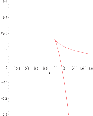
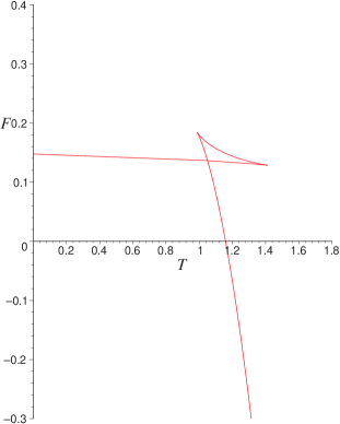
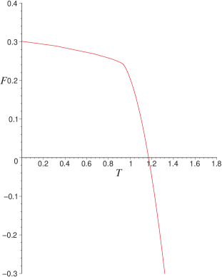
FIG. 4.: The free energy vs. temperature for the fixed charge ensemble, in a series of snapshots for varying charge, for values $Q{=}0,0.15$ and $Q{=}0.299$. Note that $Q_{\rm crit}{=}0.289$, so in the last plot, the bend (near $T_{\rm crit}{=}0.943$, is in the neighbourhood of the critical point of second order.

It may be further observed that a plot of $F(Q)$ for fixed $T$ reveals (above a $T_{\rm crit}$), a similar swallowtail section, as shown in figure 5.

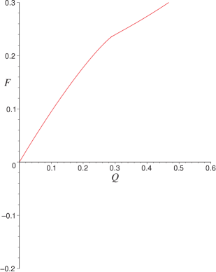
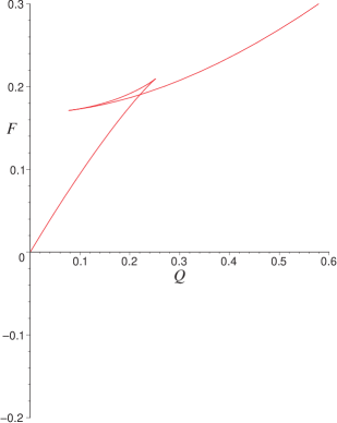
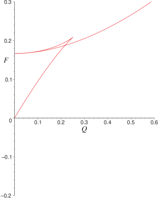
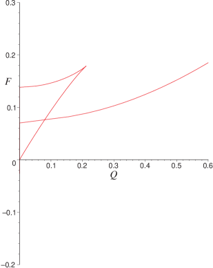
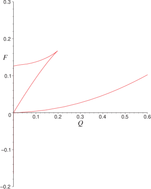
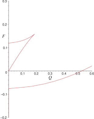
FIG. 5.: The free energy vs. charge for the fixed charge ensemble, in a series of snapshots for varying temperature, for values $T{=}0.943,0.997,1.00,1.10$, and (for the “Zorro” plot) $T{=}T_{\rm HP}{=}1.154$, and finally $T{=}1.20$. Note that $T_{\rm crit}{=}0.943$, and so in the first plot, the bend (near $Q_{\rm crit}{=}0.289$), is in the neighbourhood of the critical point of second order.

The full three dimensional shape of $F[Q,T]$ is plotted in figure 6.

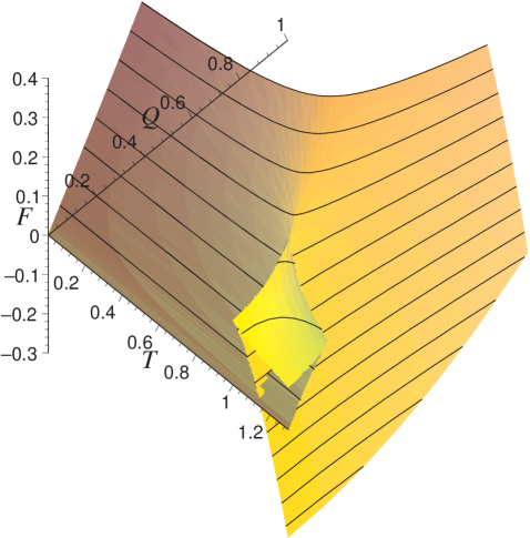
FIG. 6.: Plots of the Helmholtz potential $F[Q,T]$, in three dimensions, clearly showing the swallowtail shape for $T{>}T_{\rm crit}$ and $Q{<}Q_{\rm crit}$.

That such a shape appears in the thermodynamics (above $T_{\rm crit}$ or below a $Q_{\rm crit}$) can be shown to follow from the first law of thermodynamics, the definition of the thermodynamic potentials, and the form of the particular equations of state which the black holes obey. We will show how this comes about next.

V The swallow tales

The sections of swallowtails in the $F(Q)$ and $F(T)$ plots (above a $T_{\rm crit}$ or below a $Q_{\rm crit}$) can be seen to come from the existence of the previously mentioned three branches of solutions to the equation of state. We have from the first law, and the definition of the thermodynamic potential, that $dF{=}{-}SdT{+}\Phi dQ$. Therefore, for fixed $T$ we find

$$F(T)=\int\Phi(Q)\,dQ+f(T)\ ,$$ (26)

where $f(T)$ is an arbitrary function of $T$. The integral function can be obtained by looking at the plot of isotherms. When we have three branches (i.e., $T{>}T_{\rm crit}$), the curve $\Phi(Q)$ winds back and forth in a way that the integral describes a shape with three connected branches, constituting a section of the “swallowtail” shape. This can be seen by examination of the plots of the equation of state in figure 1 and the plots of the slices $F(T)$ displayed in figure 4.

Equation (26) is usually employed to formulate an “equal area law” governing the phase transitions of the system. The latter occur at the point where the free energies of two branches, (say A and B), are equal: $F_{\rm A}{=}F_{\rm B}$. From eqn. (26) this equality may be translated into a statement about the equality of the areas enclosed by the isotherm curves and a line of constant $Q$ in the $(\Phi,Q)$ plane, as shown in the sketch on the left in figure 7. There is a subtlety, though, in using eqn. (26) with the isotherm curves of eqn. (17) for $T{>}1$ (recall that isotherms with $T{\geq}1$ go through the origin $\Phi{=}Q{=}0$. See figure 1.). Given that the transition is governed by the equal area law, it would seem from the curves on the right in figure 7 and the area law deduced from eqn. (26) that even for $T{>}1$, for which a minimum value of $\Phi$ ceases to exist, one can always find a phase transition point for arbitrarily large temperatures and small enough charge. This must be wrong since it contradicts what we know about the phase transition from the curves of $F$ for constant $Q$, namely, that the phase transition takes place at a temperature that is smaller (or equal, at $Q{=}0$) than the Hawking–Page temperature $T_{\rm HP}$. (See ref.[17] and the upcoming section VII for detailed discussion of the phase structure.)

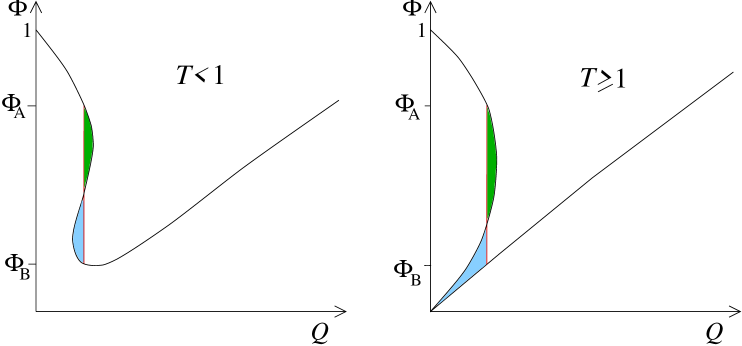
FIG. 7.: The figure on the left shows how the condition for a phase transition may be interpreted in terms of an “equal area law” analogous to that due to Maxwell for the van–der Waals liquid–gas model. For $T{\geq}1$, though, the isotherms have a very different qualitative structure. The equal area law one might formulate, deducing a phase transition for arbitrarily high $T{>}1$, for small enough $Q$, actually is incorrect. See text for the resolution of the puzzle.

The resolution of this puzzle is instructive, and is made manifest most clearly by working in terms of the parameter $r_{+}$, using eqns. (19), (20) and (24). We can explicitly compute $F$ using eqn. (26) as

$$F=\int_{0}^{r_{+}}\Phi(\bar{r}_{+})(dQ/d\bar{r}_{+})d\bar{r}_{+}$$ (27)

to recover precisely eqn. (24). So, what is the reason that “naive integration” using the “the equal area law” yields a different result?

The point is that for $T{>}1$ the function $F(Q)$ is discontinuous at $Q{=}0$, where branches 2 and 3 separate (see for example, the last plot of figure 5). For those isotherms, there is a range of values for $r_{+}$, $T{-}\sqrt{T^{2}{-}1}{<}r_{+}{<}T+\sqrt{T^{2}{-}1}$ for which $Q$ and $\Phi$ become imaginary. Nonetheless, the product $\Phi dQ$ is real throughout, and so is $F$. Then, $F(Q)$ would be a continuous function if we plotted it in the complex $Q$ plane. In performing the integration above for $T{>}1$ we have implicitly included the points where $\Phi$ and $Q$ are imaginary. Notice that it is by including these points that we recover sensible physics, since we want the critical line to end at $Q{=}0$ at the point of the Hawking–Page phase transition. The “equal area law”, as it is, fails in this instance.

Let us now turn to the study of the free energy for fixed $Q$. We have

$$F(Q)=-\int S(T)dT+g(Q)$$ (28)

In this case we need $S(T)$. Since

$$S={1\over 2}\left({Q\over\Phi}\right)^{2}={r_{+}^{2}\over 2}$$ (29)

we can use the equation of state to plot $S(T)$ for fixed $Q$, which is shown in figure 8.

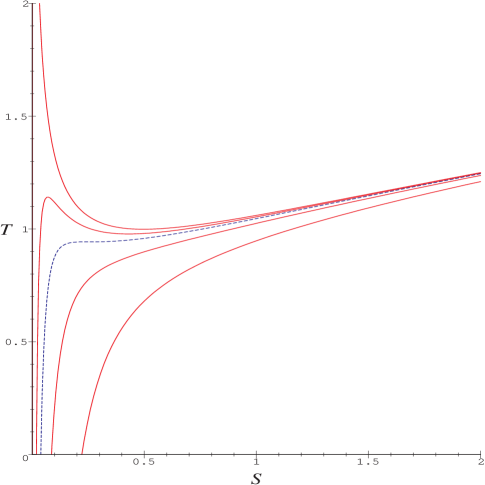
FIG. 8.: Plots of the equation of state of $S$ vs. $T$, showing isocharge lines above and below the critical charge $Q_{\rm crit}$. For $Q{>}Q_{\rm crit}$, there is only one branch of solutions, while for $Q{<}Q_{\rm crit}$, there are three branches. The values of $Q$ for the isocharge curves plotted are (top down) $Q{=}0,0.20,Q_{\rm crit},0.45,0.80$. (The uppermost curve shows the $Q{=}0$ case, which has two branches. The central (dotted) curve is at the critical charge.

It can be readily seen that for $Q{<}Q_{crit}$ we get three branches (notice that the qualitative features of the plot of $S(T)$ follow from those of $r_{+}(T)$ or $r_{+}(\beta)$ plotted in figure 3 of ref.[17], where it has a resemblance to the van der Waals $P(V)$ curve). A section of the swallowtail again follows.

The astute reader may wonder why the swallowtail shape (and the resulting liquid–gas–like) phase diagram occurs in the canonical ensemble, where in addition to $T$, the extensive variable $Q$ is an external control parameter, and not in the grand canonical ensemble, where the intensive variable $\Phi$ would be the control. This is of course what happens in the case of the van–der–Waals–Maxwell system, where the phase diagram is in $(P,T)$ space, and not $(V,T)$ space[26, 27]. The swallowtail shapes occur there in the Gibbs potential. It is now hopefully clear that the answer follows from the fact that our equation of state yields three branches of solutions for the intensive variable $\Phi$ (or T) as a function of the fixed extensive variable $Q$ (or $S$), as can be seen by examining the curves displayed in figs. 1 and 8.

That there are no swallowtail shapes in any of the other ensembles follows from the fact that no more than two branches occur for the equation of state written in terms of other variables.

VI intrinsic stability

Given that we have the full power of the thermodynamic framework at our disposal, (thanks to the stabilizing influence of a negative cosmological constant), it is interesting to consider the thermodynamic stability of our various solutions against microscopic fluctuations. Notice that one can always formally compute the relevant macroscopic quantities (like specific heats, etc.,) which we discuss here, without any reference to an underlying microscopic description. This has been done in the context of black hole thermodynamics since time immemorial. The difference here is that we know the nature of the microscopic degrees of freedom which supply the underlying “Statistical Mechanics” which gives rise to these macroscopic thermodynamics quantities. The underlying physics is that of the gauge theory to which this system is holographically dual, which in turn is the physics of coincident branes. This will become more apparent in section IX when we explicitly study the fluctuations themselves.

Thermodynamic stability may be phrased in many different ways[30, 31], depending on which thermodynamic function we choose to use, and how obscure we are attempting to seem. For example, it can be seen as minimization of the energy, $E$, as a function of $(S,Q)$, or maximization of the entropy $S$, as a function of $(E,Q)$, etc. In any case, one is considering an infinitesimal variation of the state function away from equilibrium. The first law (15) will ensure that the first order terms vanish. Stability is then a statement about the second order variations. Generally then the stability conditions are phrased in terms of the restriction that the Hessian of the state function is positive (or negative, depending on the context) semi–definite.

An equivalent but physically more transparent way of writing the stability conditions is in terms of specific heats and other “compressibilities”, to wit:

$$C_{Q}\equiv T\left({\partial S\over\partial T}\right)_{Q}\geq 0,\quad C_{\Phi}\equiv T\left({\partial S\over\partial T}\right)_{\Phi}\geq 0,\quad\varepsilon_{T}\equiv\left({\partial Q\over\partial\Phi}\right)_{T}\geq 0\ .$$ (30)

The first two, the specific heats at constant electric charge and potential, are familiar analogues of the specific heats at constant volume and pressure in fluid systems. In the case in hand, they determine the thermal stability of the black holes, indicating whether a thermal fluctuation results in an increase or decrease in the size of the black hole. (This follows from the fact that the entropy is proportional to the size of the black hole,.) Stability follows from $C{\geq}0$, given the fact that black holes radiate at higher temperatures when they are smaller.

The last quantity, $\varepsilon_{T}$, has the following physical interpretation. It is negative if the black hole is electrically unstable to electrical fluctuations (if they are possible, see later discussion). This happens if the potential of the black hole decreases as a result of placing more charge on it. The potential should of course increase, in an attempt to make it harder to move the system from equilibrium. $\varepsilon_{T}$ therefore deserves to be called the “isothermal (relative) permittivity” of the black hole.

There are of course other interesting “response functions” for the system, such as the adiabatic permittivity, $(\partial Q/\partial\Phi)_{S}$ or the quantity analogous to the coefficient of thermal expansion in liquid–gas systems, $\alpha_{\Phi}{=}(\partial Q/\partial T)_{\Phi}$, which are not all independent. The ones which we have discussed above will suffice for the physics that we study in this paper.

We may examine the plots of the isotherms in figure 1 and deduce that the negatively sloped branches are electrically unstable if there are electrical fluctuations possible. Similarly, we may deduce that the negatively sloped branches of the $(S,T)$ isocharge curves in figure 8, are thermally unstable, and so on.

Stability follows, equivalently, from the concavity/convexity of the plots of $F$ and $W$ as functions of $T$. In fact, the specific heat conditions are equivalent to

$$\left({\partial^{2}F\over\partial T^{2}}\right)_{Q}\leq 0\quad{\rm and}\quad\left({\partial^{2}W\over\partial T^{2}}\right)_{\Phi}\leq 0\ ,$$ (31)

whereas the permittivity condition is

$$\left({\partial^{2}F\over\partial Q^{2}}\right)_{T}\geq 0,\quad{\rm or}\quad\left({\partial^{2}W\over\partial\Phi^{2}}\right)_{T}\leq 0\ .$$ (32)

By examining the isotherms displayed in figure 1, we see that there are a number of features in the $(Q,T)$ plane which govern electrical stability. Generically, let us describe the three branches of an isotherm as follows: We call “branch 3” the branch of solutions which extends all the way from $Q{=}\infty$, terminating where $dQ/d\Phi{=}0$. From there, “branch 2” takes over, terminating where again $dQ/d\Phi{=}0$. The isotherm continues with “branch 1” until the point $Q{=}0,\Phi{=}1$ is reached. This terminology matches that of ref.[17].

From this definition, then, branch 3 is electrically stable for most of its extent, except for a small region near the join with branch 2. In this case, before reaching the point where $dQ/d\Phi{=}0$ the permittivity changes sign at a point where $dQ/d\Phi{=}\infty$ and renders branch 3 electrically unstable thereafter. This is a feature that is absent from the standard van–der–Waals–Maxwell system (in the latter there are no points in the isotherms where $dP/dV=\infty$), and which will introduce a significant modification of the phase diagram.

Branch 2, being between two places where $dQ/d\Phi{=}0$, has positive definite slope and hence is electrically stable everywhere, while branch 1 is electrically unstable everywhere, having negative definite slope. To compute precisely where the electrical instability begins, we need only find the location of the minimum of the isotherms, that is, the above mentioned point where $dQ/d\Phi{=}\infty$, which is given by the equation $Q{=}T\sqrt{1{-}T^{2}}$. With the segment of the $T$–axis from 0 to 1, this forms a region in the $(Q,T)$ plane within which branch 3 and branch 1 are unstable to electric fluctuations. Branch 2 is electrically stable everywhere, as mentioned before, but as already pointed out in ref.[17], and as a quick examination of the figure 8 of the isocharge $(S,T)$ curves reveals, branch 2 is unstable to thermal fluctuations, and so never plays a role in the canonical and grand canonical ensembles.

It is also entertaining to subject by eye the snapshots of $F$ and $W$ taken in figures 3, 4 and 5 to the convexity and concavity conditions (31) and (32). We find that the shapes of $F$ and $W$ do indeed confirm our conclusions about the stability of the various branches.

It is very instructive to plot the boundaries of the various branches in the $(Q,T)$ plane:

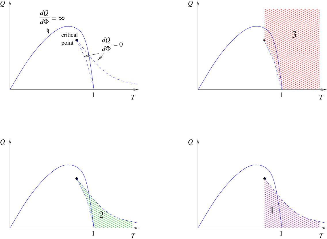
FIG. 9.: The demarkation of the various branches of black holes in the $(Q,T)$ plane. Points on branches 1 and 3 which lie inside the solid curved line are unstable to electric fluctuations. Branch 2 is electrically stable but thermally unstable everywhere.

It is particularly interesting to note that the figures in the previous plot are simply the three sheets of an underlying “cusp catastrophe” shape, as can be seen by assembling them in three dimensions to reconstruct the equation of state in figure 1. Indeed, it is highly instructive to align the surface $\Phi(Q,T)$ describing equation of state and the surface $F[Q,T]$ giving the swallowtail shape of the free energy, in such a way as to project some of their important features to the $(Q,T)$ plane, as done in figure 10. This gives rise to the critical phase diagram which we will discuss in the next section.

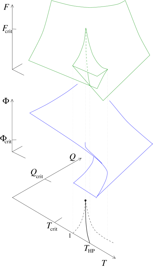
FIG. 10.: The swallowtail shape (free energy) and cusp shape (equation of state) for the charged black hole thermodynamic system. Notice the features which result in the critical line and point in the $(Q,T)$ plane.

As anticipated, the shape formed by the equation of state in the neighbourhood of the critical point is merely a distortion of the standard cusp shape, which was encountered in the variables $(r_{+},Q,\beta)$ in our previous paper [17]. Figure 11 shows this standard shape with two sample trajectories in state space. It will be discussed further in section XI.

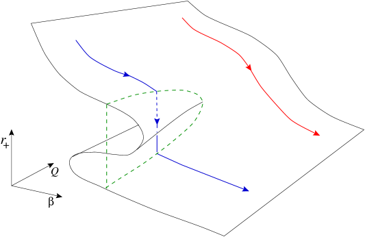
FIG. 11.: A sketch of the cusp catastrophe in action (in $(r_{+},Q,\beta)$ space). Two sample trajectories are shown, one ($Q{<}Q_{\rm crit}$) encountering a phase transition, the other ($Q{>}Q_{\rm crit}$) does not. The precise location of the line across which the transition happens is given by the minimum free energy condition, or equivalently, an appropriately formulated “equal area law”.

As a final comment that in cases where one of the local stability criteria (30) are violated, we are not always able to determine the stable ground state. However, the precise nature of the stability violation is providing information about how the system will relax to a new stable configuration. For example, one has $\delta^{2}E{\propto}\varepsilon_{T}\,\delta Q^{2}$ and so $\varepsilon_{T}{<}0$ indicates that the black hole should relax by reducing its charge, i.e., it will emit charged particles (if possible).

VII Phase structure

Figures 10 and 6, together with the slices displayed in figures 4 and 5, show how the free energy curve determines the phase structure of the black holes as one moves around on the state curve in the canonical ensemble, while figures 2 and the slices displayed in figure 3 determine the phase diagram for the grand canonical ensemble. We performed this analysis in ref. [17], and we recall it here for completeness, before going on to refine the resulting phase diagram using the information uncovered in this paper.

The dashed line in the $(Q,T)$ plane shows the boundary of the region multiply covered by $\Phi$, in the state curve, and correspondingly, the free energy has three possible values in that region also (see fig. 10), which constitutes the swallowtail region. The free energy of branch 2 is always greater than that of either branches 1 or 3, however, and so there is no transition along the dashed lines. Along the solid line, the free energies of branches 1 and 3 are equal, and there is a first order phase transition (the first derivative of the free energy is discontinuous) along this line. Also note that the one dimensional $Q{=}0$ situation is the familiar Hawking–Page transition[13] between AdS and AdS–Schwarzschild, which happens (in our units) at $T{=}T_{HP}{=}2/\sqrt{3}{\approx}1.154$, for $n{=}3$.

The solid line is the “coexistence curve” of the two phase of allowed black hole. The line ends in a critical point. Above this point, there is no transition, and one goes from large to small black holes continuously (the distinction between branch 1 and branch 3 is removed). (The reader should compare this to the physics of the liquid–gas system for an exact analogue in classic thermodynamics.) As the first derivative (but not the second) of the free energy $F$ is continuous at the critical point, there is a second order phase transition there, about which we will have some more to say in sections IX and XI.

This physics is all summarized in figure 12, where we have also displayed the phase diagram in the grand canonical ensemble (the $(\Phi,T)$ plane), which is straightforward to determine. Some of the details of the shape of these curves will be confirmed by calculations in section VIII. For most of the rest of the paper, we will not have much more to say about the phase diagram in the $(\Phi,T)$ plane, and refer the reader to ref.[17] for discussions of its features. Note, however, that the boundary in this figure marks the line where the Gibbs free energy of the black holes equals that of AdS. That is the boundary does not denote a curve where one of the local stability criteria begins to be violated.

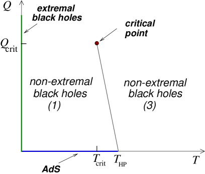
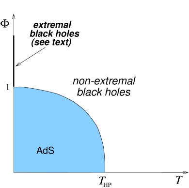
FIG. 12.: Sketches of the thermally stable phases in the canonical ensemble, and in the grand canonical ensemble, respectively.

Depending upon the situation, there may or may not be the possibility of electrical fluctuations. This depends very much upon the setting within which we are considering these black holes. In a theory without charged particles, the black hole charge would be fixed and electrical stability need not be considered. In general, however, if there are fundamental charged quanta in the theory, then there is the possibility of the black holes emitting or absorbing such quanta, introducing the possibility of electrical fluctuations. Such a possibility must be considered in (for example) the case when the EMadS system is considered to be a Kaluza–Klein truncation of some higher dimensional theory, as discussed in our previous work[17]. Then, the electrically charged black hole can in principle emit or absorb electrically charged Kaluza–Klein particles in order to allow its charge to fluctuate.

In the particular case of four dimensions, however, there is also the possibility that we can exchange, by electric–magnetic duality, the electric charge (and vector potential) that we have been considering here for a magnetic charge (and vector potential). In this case, we have instead that the only way for the magnetically charged black holes to change their charge is to emit or absorb Kaluza–Klein monopoles, which are not fundamental quanta, as they are very massive, the further we are below the Kaluza–Klein scale.

In general, when there are allowed electrical fluctuations (by whatever mechanism is appropriate to the situation in hand) we must also take into account on the phase diagram, the electrical stability of the solutions as determined in the previous section. Including those regions, we obtain the following phase diagram:

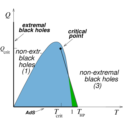
FIG. 13.: The phase diagram in the canonical ensemble, showing the disallowed (shaded) regions where the solutions are unstable to electrical fluctuations. Note that the critical point and part of the coexistence line lies within the unstable region.

The question arises as to what the equilibrium system is which resides in the shaded regions. The electrically unstable black holes cannot reside there, and so we must search for other possibilities. One formal possibility is that extremal black holes reside there, because formally they can exist at any temperature for any charge. However, we do not find this possibility very attractive. We expect that the permission that the Euclidean computation appears to give them to exist at any temperature is an artifact, and that they should naturally be associated with zero temperature, in which case they can only occupy the line $T{=}0$ on our phase diagram in the canonical ensemble, which they do. In any event, one can infer from the calculations of ref. [17] that extremal black holes actually have a higher free energy than the unstable nonextremal black holes. Another possibility is that the preferred state is simply anti–de Sitter space (which can also exist at arbitrary temperature) filled with a charged gas. This is certainly the case at $Q{=}0$ [11, 13]. However, when the gas carries a non–negligible charge (and hence mass), its backreaction on the AdS geometry can not be neglected in determining the free energy. Another interesting possibility is that of black hole surrounded by a gas of particles. Again, if the gas component carries a sizable fraction of the charge and mass, its backreaction on the geometry would modify the equation of state and may then re–establish thermodynamic stability. Pursuing either of these possibilities lies beyond the scope of the present paper, and so we will leave settling of this interesting issue to a future date. Hence we must simply regard the shaded region as a sort of terra incognita with regard to black hole physics. As a final note, we remind the reader that this is only the region in which we are certain that the black holes do not minimize the free energy due to its thermodynamic instability. It may be that the onset of a phase transition to a state of lower free energy actually occurs outside of the boundary in figure 13, just as it does for the grand canonical ensemble in figure 12.

VIII Coexistence of phases and the Clapeyron equation

Let us study further the coexistence lines which we discovered in the phase diagrams, both in the canonical ensemble and in the grand canonical ensemble (see figure 12). We can use straightforward thermodynamics to determine the shape of the lines.

Let us start with the grand canonical ensemble, with Gibbs potential $W[\Phi,T]$, with $dW{=}{-}SdT{-}Qd\Phi$. An equation can be derived for the line separating two phases A and B in the $(\Phi,T)$ phase diagram as follows. Along such a coexistence line the phases (for given $(\Phi,T)$) have the same $W$, and so the slope of the curve $Q(T)$ is related to the change in entropy and $Q$ by:

$${d\Phi\over dT}=-{S_{\rm A}-S_{\rm B}\over Q_{\rm A}-Q_{\rm B}}\ .$$ (33)

In the case at hand, one of the phases is AdS which has zero entropy and zero charge. So we find that (for all $n$):

$${d\Phi\over dT}=-{S_{\rm bh}\over Q_{\rm bh}}=-\left({2\pi\over n-1}\right){1\over cq}\left({q\over c\Phi}\right)^{n-1\over n-2}\ .$$ (34)

Here, $q(T,\Phi)$ is obtained from the equation of state for the corresponding branch. Equation (34) is the precise analogue of the Clapeyron equation. From it, we see that the slope of the curve is negative. For the case of $n{=}3$ we can give explicit expressions. In the rescaled units, we have:

$${d\Phi\over dT}=-{Q\over 2\Phi^{2}}=-{1\over 2}\left({T\over\Phi}+\sqrt{{T^{2}\over\Phi^{2}}+1-{1\over\Phi^{2}}}\right)\ .$$ (35)

We see from here that the curve intersects the axes orthogonally, and its convexity, sketched in the figure 12, follows from the fact that ${d^{2}\Phi/dT^{2}}{<}0$.

Next (assuming the issue of electrical stability can be ignored), we consider the canonical ensemble, defined by the Helmholtz thermodynamic potential $F[Q,T]$, with $dF{=}SdT{-}\Phi dQ$. Along any line of coexistence of two phases, we have:

$${dQ\over dT}={S_{\rm A}-S_{\rm B}\over\Phi_{\rm A}-\Phi_{\rm B}}$$ (36)

The phase diagram is sketched in figure 12.

The Clapeyron equation can be used to find the slope of the curve at $Q{=}0$ and $Q{=}Q_{\rm crit}$ for the line separating the two black holes phases (we show the expressions for all $n$):

$$\left.{dQ\over dT}\right|_{Q_{\rm crit}}=-{\omega_{n-1}\over 4G}\left({n-1\over n-2}\right){r_{+(\rm crit)}^{2n-3}\over q_{\rm crit}}\ ,$$ (37)

$$\left.{dQ\over dT}\right|_{Q{=}0}=-{\omega_{n-1}\over 4G}r_{+(3)}^{n-1}\ ,$$ (38)

(where we have used here that $r_{+(1)}^{n-2}\simeq q$ near $q=0$, as is easy to obtain). On the scale at which we have sketched the coexistence curve in the previous section, it is essentially a straight line, and we have drawn it as such in figure 12.

IX Fluctuations for Charged AdS Black Holes

In section VI, we discussed and computed the thermodynamic quantities (specific heats and permitivity) which signal the stability (or not) of a black hole against fluctuations. While these quantities pertain to the response of the system to macroscopic thermodynamic processes which may be performed, in Euclidean Quantum Gravity, where we ordinarily do not have a description of the microscopic degrees of freedom, we usually cannot relate them directly to microscopic fluctuations, as we can in ordinary thermal physics.

However, we can go further in this paper. Many of the adS models which we have here can be embedded into a full theory of quantum gravity —string and/or M–theory— and where the holographic duality tells us precisely that the microscopic description is organized neatly in terms of a dual (gauge) field theory.

So we may go and boldly study the fluctuations of the thermodynamic quantities in our theory, and we should see earmarks of the underlying (gauge) theory in our quantities, connecting the microscopic to the macroscopic.

Here, one uses the entropy to define a probability distribution on the space of independent thermodynamic quantites [31]: $p(X_{i}){\propto}\exp(S(X_{i}))$. With the assumption that fluctuations are small, we can work with a quadratic expansion of the entropy in deviations from the equilibrium values. The stability analysis of section VI establishes that the Hessian of $S$ is negative semi–definite, and so we have a normalizable Gaussian distribution within this approximation. One then finds that the fluctuations are given by

$$\langle\delta X_{i}\,\delta X_{k}\rangle=-\left({\partial^{2}S\over\partial X_{i}\partial X_{k}}\right)^{-1}$$ (39)

where $\delta X_{i}$ denotes the deviation of $X_{i}$ from its equilibrium value, and notation of the left–hand side denotes a matrix inverse.

Implicit above is the assumption that we have a closed system can be divided into a number of subsystems. In the AdS context, the natural decomposition is the black hole and the thermodynamic reservoirs. In this situation where the subsystem of interest is really the entire object under study, the most reasonable approach is to consider fluctuations in only the extensive variables that are free to vary in the thermodynamic ensemble [30]. Hence we denote the general extensive variables that are free to vary as $X_{i}$, and the $F_{i}$’s are their conjugate intensive variables defined by $dS{=}F_{k}\,dX_{k}$. Eqn. (39) then becomes[30, 31]

$$\langle\delta X_{i}\,\delta X_{k}\rangle=-{\partial X_{i}\over\partial F_{k}}=-{\partial X_{k}\over\partial F_{i}}\ .$$ (40)

Now, these fluctuations are given practical meaning when they are compared to for example, their equilibrium values. For example, the relative root mean square of the fluctuations:

$${\sqrt{\langle\delta X_{i}^{2}\rangle}\over X_{i}}$$ (41)

which tells us about the sharpness of the distribution in $X_{i}$.

Note, that by the formula (40) the above ratio goes roughly as the extensive parameters to the ${-}1/2$, and therefore the distribution is increasingly sharp as the size of the system increases.

Now in the present problem of charged black holes,

$$dS=(1/T)dE-(\Phi/T)dQ\ .$$ (42)

Hence for the canonical (fixed $Q$) ensemble (our analogue of a fixed volume system), the only free extensive variable is the energy, and the above formulae yield

$$\langle\delta E^{2}\rangle=-\left({\partial E\over\partial\beta}\right)_{Q}=T^{2}\left({\partial E\over\partial T}\right)_{Q}=T\,C_{Q}\ .$$ (43)

For the grand canonical (fixed $\Phi$) ensemble (analogue of a fixed pressure system), the energy and the charge are free to vary, and one has

$$\langle\delta E^{2}\rangle = -\left({\partial E\over\partial\beta}\right)_{\Phi/T}=T^{2}\left({\partial E\over\partial T}\right)_{\Phi/T}$$ (44)

$$= TC_{\Phi}+T\Phi\left({\partial E\over\partial\Phi}\right)_{T}\ .$$ (45)

$$\langle\delta Q^{2}\rangle = T\left({\partial Q\over\partial\Phi}\right)_{T}=T\varepsilon_{T}\ .$$ (46)

$$\langle\delta E\,\delta Q\rangle = T\left({\partial E\over\partial\Phi}\right)_{T}$$ (47)

$$= T^{2}\left({\partial Q\over\partial T}\right)_{\Phi}+T\Phi\left({\partial Q\over\partial\Phi}\right)_{T}=T^{2}\alpha_{\Phi}+T\Phi\varepsilon_{T}\ .$$ (48)

We have recovered the fact that the thermodynamic fluctuations are controlled by the same generalized compressibilities —specific heats permittivity, etc.,— that determine the intrinsic stability in section VI. This follows since both analyses can be phrased in terms of the Hessian of the entropy.

Above we have presented a general thermodynamic discussion. Let us now focus on the case $n{=}3$ and present our results in terms of the dimensionless variables introduced in section  I. Note that translating the above thermodynamic formulae to the dimensionless variables, there are extra factors, giving e.g.,

$$\langle\delta E^{2}\rangle={3G\over 2\pi l^{2}}T^{2}{\partial E\over\partial T}\ .$$ (49)

For the fixed charge ensemble:

$${\langle\delta E^{2}\rangle\over E^{2}}={3G\over 2\pi l^{2}}{1\over r_{+}^{2}}{\left({r_{+}^{2}}+1-{q^{2}\over r_{+}^{2}}\right)^{3}\over\left({r_{+}^{2}}-1+3{q^{2}\over r_{+}^{2}}\right)\left({r_{+}^{2}}+1+{q^{2}\over r_{+}^{2}}\right)^{2}}\ .$$ (50)

For the fixed potential ensemble:

$${\langle\delta E^{2}\rangle\over E^{2}}={3G\over 2\pi l^{2}}{1\over r_{+}^{2}}{\left({r_{+}^{2}}+1-\Phi^{2}\right)\over\left({r_{+}^{2}}-1+\Phi^{2}\right)}\left[{\left({r_{+}^{2}}+1-\Phi^{2}\right)^{2}+4\Phi^{2}(1-\Phi^{2})\over\left({r_{+}^{2}\over 3}+1-\Phi^{2}\right)^{2}}\right]\ ,$$ (51)

$${\langle\delta Q^{2}\rangle\over Q^{2}}={3G\over 4\pi l^{2}}{1\over\Phi^{2}r_{+}^{2}}\left[{\left({r_{+}^{2}}+1-\Phi^{2}\right)\left({r_{+}^{2}}-1+3\Phi^{2}\right)\over\left({r_{+}^{2}}-1+\Phi^{2}\right)}\right]\ .$$ (52)

$${\langle\delta E\delta Q\rangle\over{E\,Q}}={3G\over\pi l^{2}}{1-\Phi^{2}\over r_{+}^{2}}\left[{\left({r_{+}^{2}}+1-\Phi^{2}\right)\over\left({r_{+}^{2}}-1+\Phi^{2}\right)\left({r_{+}^{2}\over 3}+1-\Phi^{2}\right)}\right]\ .$$ (53)

Notice that all of these results are proportional to $G/l^{2}{\sim}N^{-3/2}$, so for large $N$ the fluctuations are suppressed. For $n{=}3$, the dual field theory (supplying our microscopic description) is the field theory of ref.[32], associated to $N$ coincident M2–branes. The number of degrees of freedom in this theory grows as $N^{3/2}$ (as seen for example in the black hole entropy at high temperature). So the squared fluctuations are controlled by the inverse of the number of degrees of freedom of the field theory, which is precisely what we expect from standard kinetic theory connecting the microscopic to the macroscopic! Note here that we see these unconfined degrees of freedom appearing in our formulae at arbitrary temperature in this ensemble. This is because black holes dominate the thermodynamics for all values of the temperature: the presence of charge effects a deconfinement of the theory at all temperatures, even in finite volume. (This is to be contrasted to the case of $Q{=}0$, where AdS dominates the physics for some $T{<}T_{\rm HP}$, representing the “confined” phase.)

To gain more insight into these results, let us rewrite eqn. (49) for the energy fluctuations as:

$${\langle\delta E^{2}\rangle\over E^{2}}={3G\over 2\pi l^{2}}{T^{3}\over r_{+}^{2}\left(T+{Q\over r_{+}^{3}}\right)^{2}}{1\over\left({\partial T\over\partial r_{+}}\right)_{Q}}$$ (54)

From this form, one can pick out some of the interesting behaviour. The fluctuations go to zero at zero temperature as $T^{3}$. For large $T$ (and hence large $E$), the fluctuations also go to zero now as $1/T$ (since for large $r_{+}$, $2T{\simeq}r_{+}$). An interesting factor is $(\partial T/\partial r_{+})^{-1}$ which can change sign for $Q{<}Q_{\rm crit}{=}1/(2\sqrt{3})$.

So for $Q{>}Q_{\rm crit}$, the fluctuations rise from zero at the extremal black ($T{=}0$) go through a maximum and then die down for large temperatures. As $Q$ approaches $Q_{\rm crit}$, the maximum grows larger and larger, and actually becomes a divergence at $Q{=}Q_{\rm crit}$! (We have plotted these squared fluctuations in figure 14, where they are denoted $f(T)$.) This is actually the same divergence as that in $C_{Q}$ at the critical point, which was commented on in ref[17]. Hence one finds from there that near the critical point,

$${\langle\delta E^{2}\rangle\over E^{2}}\sim(T-T_{\rm crit})^{-2/3}\ .$$ (55)

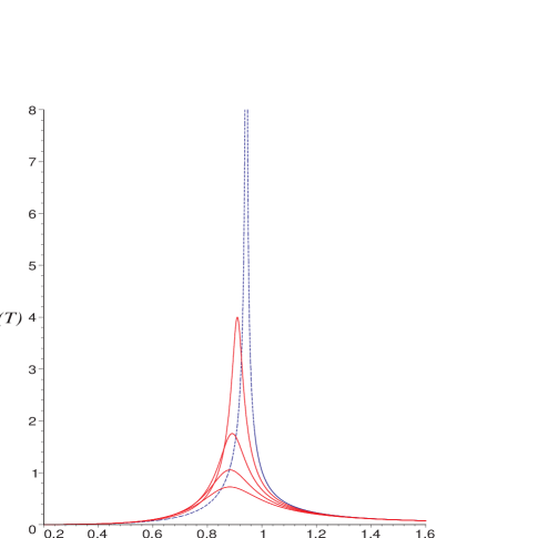
FIG. 14.: The squared fluctuations $f(T)$ in the energy, relative to the equilibrium energy, for varying $Q{\geq}Q_{\rm crit}$. The values of $Q$ plotted here are (bottom up) $Q{=}0.49,0.44,0.39,0.34,Q_{\rm crit}$. The dotted curve shows that the fluctuations diverge at $Q{=}Q_{\rm crit}$, at the critical temperature $T{=}T_{\rm crit}$.

This divergence of the energy fluctuations signals the breakdown of the Gaussian approximation considered in these calculations. It is also the classic behaviour of a second order phase transition point, where correlation lengths, etc., diverge as an order parameter vanishes. Here, the order parameter can be taken to be a homogenous function of $r_{+(3)}{-}r_{+(1)}$, the difference between horizon radii of the branches 3 and 1.

For $Q{<}Q_{\rm crit}$, the fluctuations rise from zero at the extremal black hole and diverge at the first zero of $\partial T/\partial r_{+}$. Between the two zeros of $\partial T/\partial r_{+}$, $\langle\delta E^{2}\rangle/E^{2}$ is negative. This is simply an indication that we are in the thermally unstable regime, otherwise known as “branch 2”. For $T$ larger than the second zero of $\partial T/\partial r_{+}$, the fluctuations are monotonically decreasing (from infinity at the zero, to zero as $T\rightarrow\infty$). As we know from the minimum free energy condition, we are protected from the unstable regime by making a phase transition from branch 1 and 3. So in a $\langle\delta E^{2}\rangle/E^{2}$ versus $T$ plot, the fluctuations rise from zero to the phase transition point and the (discontinuously) jump to the decreasing curve.

X Of Higher dimensions and Other thermodynamic functions and ensembles

In this section, we collect together some results for various thermodynamic quantities computed for arbitrary $n$, with all of the factors explicitly included. The thermodynamic functions are written in terms of their canonical state variables. We do not use the physical charge $Q$ instead of $q$, for simplicity of presentation. In any expression, $Q$ may be restored by recalling that

$$Q={\omega_{n-1}\over 8\pi G}(n-1)cq\quad{\rm and}\quad c=\sqrt{2(n-2)\over n-1}\ .$$ (56)

Similarly, we also introduce the parameter $s$ as

$$S={\omega_{n-1}\over 4G}s\ .$$ (57)

Notice that it does make sense to write physical quantities in terms of $q$ and $s$, since they are related to the charge and entropy densities. This follows from the fact that we may replace $l^{n-1}\omega_{n-1}$ by the field theory’s volume $V_{n-1}$.

The equation of state, following from eqn. (10) is:

$$T={(n-2)l^{2}(1-c^{2}\Phi^{2})(c\Phi)^{2\over n-2}+nq^{2\over n-2}\over 4\pi l^{2}(cq\Phi)^{1\over n-2}}$$ (58)

Equation of state for extremal black holes is:

$$q^{2\over n-2}={n-2\over n}l^{2}(c^{2}\Phi_{e}^{2}-1)(c\Phi_{e})^{2\over n-2},\qquad{\rm for}\quad T\,\,{\rm arbitrary.}$$ (59)

The Gibbs thermodynamic potential for the grand canonical ensemble is[17]:

$$W[T,\Phi]={\omega_{n-1}\over 16\pi Gl^{2}}\left[l^{2}{q\over c\Phi}(1-c^{2}\Phi^{2})-\left({q\over c\Phi}\right)^{n\over n-2}\right]$$ (60)

where $Q{=}Q(T,\Phi)$ is obtained from the equation of state. Notice that $W[T,\Phi]$ vanishes for anti–de Sitter spacetime (which has $Q{=}0$), and so AdS may be thought of as the reference background for the calculation of the action, and indeed $W[T,\Phi]$ was computed in this way in ref.[17], using the background subtraction method, which we see (in the present work) gives the same result as the intrinsic definition by “counterterm subtraction” methods.

The Helmholtz free energy which is the Legendre transform of $W[T,\Phi]$ may be computed with an explicit action calculation, using the counterterm subtraction method to give an intrinsic (“backgroundless”) definition. The result is:

$$F[T,Q]={\omega_{n-1}\over 16\pi Gl^{2}}\left[l^{2}{q\over c\Phi}-\left({q\over c\Phi}\right)^{n\over n-2}+(2n-3)l^{2}cq\Phi\right]\ .$$ (61)

Again, $\Phi{=}\Phi(T,Q)$ is obtained from the equation of state. Notice that AdS with with non–zero charge is not a solution of the equations of motion and so cannot be considered as the “ground state” or reference background for this result. Indeed, this result cannot be obtained by an action calculation which uses a matching to a background, precisely for this reason. The counterterm subtraction technique is therefore necessary here to supply the honest action computation for this thermodynamic potential. It is satisfying to note that $W[T,\Phi]$ and $F[T,Q]$ are Legendre transforms of each other, $W{=}F{+}Q\Phi$, as they should be.

We can arrive at a variety of other ensembles, with their corresponding associated potentials, by formal Legendre transforms. For example, we can consider the enthalpy $H[S,\Phi]$, a function of entropy and potential (this notation is not to be confused with the Hamiltonian!). Starting from $W[T,\Phi]$ we can construct $H{=}W{+}TS$, finding

$$H[S,\Phi]={(n-1)\omega_{n-1}\over 16\pi Gl^{2}}\left[s^{n\over n-1}+l^{2}s^{n-2\over n-1}(1-c^{2}\Phi^{2})\right]\ .$$ (62)

Notice that this function can not be obtained by performing a proper background subtraction in Euclidean gravity, since for any given solution we cannot find another regular solution with the same values of the entropy and the potential. However, the enthalpy vanishes for AdS, which could therefore be regarded as the ground state or reference background here.

Another thermodynamic function in terms of its canonical variables is the (internal) energy $E{=}W{+}TS{+}Q\Phi$,

$$E[S,Q]={(n-1)\omega_{n-1}\over 16\pi Gl^{2}}\left[s^{n\over n-1}+l^{2}s^{n-2\over n-1}+q^{2}l^{2}s^{-{n-2\over n-1}}\right]\ ,$$ (63)

which vanishes as well for AdS. This function would define the thermodynamic potential for the microcanonical ensemble, and as for the enthalpy above, a calculation from Euclidean gravity should proceed by fixing the entropy of the state–the black hole area, if we neglect the entropy of the charged gas in AdS.

XI The Universal Neighbourhood of the Critical Point

In the section IX, we saw that fluctuations diverge as we approach the critical point in the canonical ensemble. This point represents a second order phase transition, as can be seen from the fact that the free energy’s first derivative ceases to have a discontinuity there (see figures 4 and 5 for visual confirmation), while the divergences of the last section signals a discontinuity in the second derivative.

While much of the detailed discussion of the paper has been for $n{=}3$, we emphasize here again that the results extend to all $n{>}2$. This is most clearly seen from the important features of the equation of state. Let us examine some of these more closely.

Consider equation (10). Originating as the condition for Euclidean regularity, and hence thermodynamic equilibrium, the qualitative features of $\beta(r_{+})$ for varying $q$ are shown in figure 15. These features are the same for all $n$: There is a critical charge, $q_{\rm crit}$, below which there are three solutions for $r_{+}$ for a range of values of $\beta$, corresponding to the small (branch 1), branch 2, and large (branch 3) black holes, in the language of ref.[17], and in this paper.

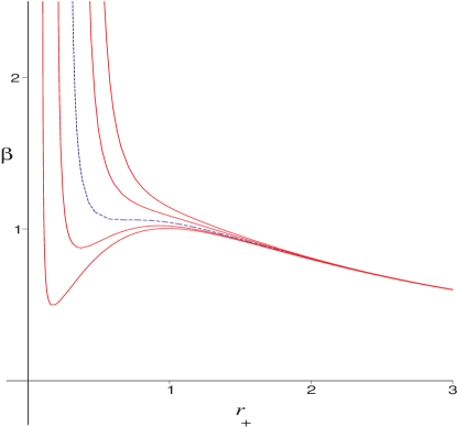
FIG. 15.: A family of isocharge curves for the $(\beta,r_{\rm+})$ form of the equation of state. Note that the middle curve is for the critical value of the charge, $Q_{\rm crit}$, below which multiple branches of $r_{\rm+}$ solutions appear. The neighbourhood of the critical point is a universal cubic, true for all dimensions.

That this shape persists for arbitrary $n$ can be seen as follows. First, note that for large $r_{+}$, $\beta(r_{+})$ goes as ${\sim}1/r_{+}$. Secondly, note that the denominator of the right hand side of eqn. (10) after choosing scalings similar to those done for $n{=}3$ at the beginning of section III, is

$$r_{+}^{2n-2}+r_{+}^{2n-4}-q^{2}=0\ ,$$ (64)

which has a single positive root, $r_{e}$, where $\beta$ diverges. This corresponds to the $T{=}0$ situation, and $r_{e}$ is the radius of the corresponding extremal black hole. Given the above, any turning points for finite $r_{+}$ must come in pairs, and the condition $\partial\beta/\partial r_{+}{=}0$ shows that there are only two real, positive such solutions, which we call $r_{+(1)}$ and $r_{+(3)}$, labeling where branch 1 ends and, respectively, where branch 3 begins. Branch 2 lies between these roots. The equations determining those roots also have an elegant form (for the same rescaling as before):

$$r_{+}^{2n-2}-r_{+}^{2n-4}+(2n{-}3)q^{2}=0\ .$$ (65)

The two roots coalesce at the critical point (i.e., $\partial^{2}\beta/\partial r_{+}^{2}{=}0$ also) where $q{=}q_{\rm crit}$. The value of the radius of this critical black hole is $r_{+({\rm crit})}$ and it is at (inverse) temperature $\beta_{\rm crit}$. For example, in the case $n{=}3$, the quantities $\{q_{\rm crit},r_{+({\rm crit})},\beta_{\rm crit}\}$ take the values $\{1/\sqrt{12},1/\sqrt{2},3/(2\sqrt{2})\}$, while for $n{=}4$, they have the values $\{2/\sqrt{135},\sqrt{(2/3)},5/(4\sqrt{6})\}$. The basic point here is that while the critical values themselves vary, the important structures do not depend upon $n$ in any essential way.

The neighbourhood of the critical point is extremely interesting. Because of the fact that for all $n$, there at most two turning points below $q_{\rm crit}$, it is clear that this neighbourhood can be better written as a cubic, in terms of local coordinates near the point. To this end, write $\rho{=}r_{+}{-}r_{+({\rm crit})}$, ${\hat{\beta}}{=}\beta{-}\beta_{\rm crit}$, and ${\hat{q}}{=}q{-}q_{\rm crit}$, and rewrite the equation of state in these coordinates. The neighbourhood of the critical point is found by taking these coordinates $(\rho,{\hat{\beta}},{\hat{q}})$ to be small.

For the example of $n{=}3$, after some algebra, we obtain

$$0=\left(\sqrt{2}-{1\over\beta}\right)\rho^{3}+2{\hat{\beta}\over\beta}\rho^{2}+\sqrt{2}{\hat{\beta}\over\beta}\rho-{\hat{q}\over 2\sqrt{3}}+{1\over 3}{\hat{\beta}\over\beta}\ .$$ (66)

Note that the quadratic and linear terms vanish with at the approach to the critical temperature ${\hat{\beta}}{\rightarrow}0$, and the term which contains $\rho^{3}$ does not vanish in this way, and so we neglect higher powers of $\rho$ in favour of this one in order to study the near–critical behaviour. Here, and in what follows, we will also neglect terms which are not linear in ${\hat{q}}$ and $\hat{\beta}$. This cubic form (66) may always be obtained in this limit for all $n$, because of the observations made in the preceding few paragraphs. From this, certain universal behaviour can be easily deduced, such as the critical exponent characterizing how fast our “order parameter”, $\rho$, vanishes. (Recall that $\rho$ represents the difference in equilibrium radius between the black holes of branch 1 and that of branch 3; it measures the distance from the analogue of the “fluid” phase in liquid–gas language, where the two forms are indistinguishable.) Setting ${\hat{\beta}}{=}0$, we see that the critical exponent is $1\over 3$, since

$$\rho\simeq\left({3\over 8}\right)^{1\over 6}{\hat{q}}^{1\over 3}\sim(Q-Q_{\rm crit})^{1\over 3}\ .$$ (67)

Performing this computation for other $n$ will change the numerical prefactor, but not the exponent, which in this sense deserves to be called universal.

That a cubic equation controls the phase structure can be traced back a step further. First, notice that the three dimensional plot of the curve in $(\beta,r_{+},Q)$ space is the cusp catastrophe, as drawn in figure 11, with some sample state space trajectories. We can remove the quadratic term in our cubic polynomial by shifting $\rho$ by an appropriate amount. Multiplying overall by a normalizing factor, our cubic may be written as:

$$0 = \rho^{3}+A\rho+B\ ,$$ (68)

$${\rm with}\quad A \simeq 4\sqrt{2}{\hat{\beta}}\quad{\rm and}\quad B\simeq{4\over 3}{\hat{\beta}}-\sqrt{3\over 2}{\hat{q}}\ .$$ (69)

Equation (68) is actually telling us about the location of the turning points of a quartic function

$${\cal V}(\rho)={1\over 4}\rho^{4}+{A\over 2}\rho^{2}+B\rho\ ,$$ (70)

where we have discarded an arbitrary additive constant. Treated as a potential, (for reasons which will be clear below), it is the generic form of ${\cal V}(\rho)$ as $A$ and $B$ vary that controls much of the critical behaviour in the neighbourhood of the critical point. (As $A$ and $B$ are functions of $Q$ and $T$, this critical behaviour in $(A,B)$ space translates directly into the earlier discussed critical behaviour in $(Q,T)$ space.)

The function ${\cal V}(\rho)$ deserves to be treated an effective potential which organizes the description of much of the local physics. In particular, away from the critical point, where $A$ and $B$ are both non–zero, the potential generically has two minima and one maximum, the location of which are given by the solutions of our universal cubic. These locations may be smoothly visualized in the form of the cusp, sketched in figure 11. The location of the minima in $\rho$ are the values $r_{+(1)}$ and $r_{+(3)}$, of the equilibrium black hole radii of branch 1 and branch 3, while the location of the maximum is $r_{+(2)}$, the branch 2 black hole radius. The thermal stability of the branches correlates with the whether the turning point is a maximum or a minimum of ${\cal V}(\rho)$, further justifying its treatment as a potential.

The boundary of the region where there are three solutions marks the situation where one of the minima of the potential ${\cal V}(\rho)$ merges with the maximum and disappears. This boundary is simply given by the values of $A$ and $B$ where the cubic’s discriminant, $\Delta{=}27B^{2}{+}4A^{3}$, vanishes. (This can only happen for $A{<}0$, therefore telling us that we have the distinct branches below $\beta_{\rm crit}$.) The interior of this region may be translated into $(Q,T)$ space, where it gives the shaded region in the third diagram of figure 9 where branch 2 resides.

Along the line in the $({\hat{q}},{\hat{\beta}})$ plane (or the $(Q,T)$ plane) where $B$ vanishes, given by ${\hat{q}}{=}\sqrt{(32/27)}{\hat{\beta}}$, the two minima of the potential ${\cal V}(\rho)$ are degenerate. This is the point at which there is phase transition, as the system moves from one minimum of the potential to the other.

At the critical point, $(A{=}0,B{=}0)$, the maximum and the two minima merge into a single minimum of the potential. Notice that the well formed by the potential is very flat there, and so the range of allowed fluctuations within it is larger at this point than at any other point in the plane, as they are less confined. We have seen this physics before as the divergence of the fluctuations of the microscopic degrees of freedom at the critical point. The potential ${\cal V}(\rho)$ is an effective potential for the uncharged microscopic degrees of freedom of the theory in the neighbourhood of the critical point. (See figure 16 for a summary of these critical points of the potential.)

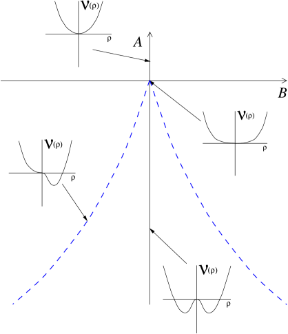
FIG. 16.: The behaviour of the Landau–Ginzburg $A_{3}$ potential at various points in the $(A,B)$ plane. This plane maps to the $(Q,T)$ plane of the charged black holes system. The line $(A{<}0,B{=}0)$, maps to the critical coexistence line found in that system.

Also, in this language, the meaning of the swallowtail shape for the thermodynamic potential $F[Q,T]$ is now clear: It is simply the actual value of the potential ${\cal V}(\rho;{\hat{\beta}},{\hat{q}})$ at its maxima and minima: the critical line is the place where these two values at the minima are equal, the place where ${\cal V}$ has degenerate minima.

This function ${\cal V}(\rho)$ is the $A_{3}$ Landau–Ginzburg potential. The effective Landau–Ginzburg theory which we can write here is an effective theory of the uncharged microscopic degrees of freedom underlying the thermodynamics. Kinetic terms to complete the Landau–Ginzburg model would have their origins in the holographically dual field theory. One can in principle derive additional potential terms governing the charged degrees of freedom as well, in order to model the stability structure uncovered in section VI, but we will not do that here.

In the language of catastrophe theory[18], the term $\rho^{4}$ is the basic “germ” of the cusp catastrophe, and $A$ and $B$ are the “unfolding parameters” which deform the potential, giving a line of first order phase transition points along the line $(B{=}0,A{<}0)$ where its mimima are degenerate. The ($A$–$D$–$E$) classification of such potentials is isomorphic to that of certain geometrical singularities[34]. We cannot help but wonder if this story marks the beginning of a richer tale involving a more profound underlying geometrical structure into which this physics is all embedded. As all of the physics of this paper is intimately connected to the physics of branes, perhaps the possibility of such a connection should be pursued.

References

References

- [1] G.W. Gibbons and S.W. Hawking, Phys. Rev. D15, 2752 (1977).
- [2] See for example, “Euclidean Quantum Gravity”, Eds, G.W. Gibbons and S.W. Hawking, World Scientific, 1993.
-
[3]
J.D. Bekenstein,
Phys. Rev. D7, 2333 (1973);
J.D. Bekenstein, Phys. Rev. D9, 3292 (1974). -
[4]
S.W. Hawking,
Commun. Math. Phys. 43, 199 (1974);
S.W. Hawking, Phys. Rev. D13, 191 (1976). -
[5]
For reviews, see:
J. Polchinski, S. Chaudhuri and C.V. Johnson, “Notes on D–branes”, hep-th/9602052;
J. Polchinski, “Tasi lectures on D–branes”, hep-th/9611050;
C.P. Bachas, “Lectures on D–branes”, hep-th/9806199;
C.V. Johnson, “Etudes on D-branes” , hep-th/9812196. - [6] For a review, see A.W. Peet, “The Bekenstein formula and string theory (N-brane theory)”, Class. Quant. Grav. 15, 3291 (1997) hep-th/9712253.
-
[7]
See reviews in:
M.J. Duff, “M theory (The Theory formerly known as strings)”, Int. J. Mod. Phys. A11, 5623 (1996) hep-th/9608117;
J.H. Schwarz, “Lectures on superstring and M theory dualities”, Nucl. Phys. Proc. Suppl. 55B, 1 (1996) hep-th/9607201. - [8] J. Maldacena, Adv. Theor. Math. Phys. 2 (1998) 231, hep-th/9711200
- [9] S. S. Gubser, I. R. Klebanov, and A. M. Polyakov, Phys. Lett. B428 (1998) 105, hep-th/9802109.
- [10] E. Witten, Adv. Theor. Math. Phys. 2 (1998) 253, hep-th/9802150.
- [11] E. Witten, Adv. Theor. Math. Phys.2 (1998) 505, hep-th/9803131.
-
[12]
G. ’t Hooft, gr-qc/9310026;
L. Susskind, J. Math. Phys. 36 (1995) 6377, hep-th/9409089. - [13] S.W. Hawking and D.N. Page, Commun. Math. Phys. 87, 577 (1983).
- [14] C. V. Johnson, Mod. Phys. Lett. A13 (1998) 2463, hep-th/9804201.
- [15] O. Aharony, M. Berkooz, D. Kutasov and N. Seiberg, J.H.E.P. 9810 (1998) 004, hep-th/9808149.
- [16] See the fourth entry of ref.[5] for further discussion in a wider context.
- [17] A. Chamblin, R. Emparan, C. V. Johnson and R. C. Myers, hep-th/9902170, to appear in Phys. Rev. D.
- [18] See for example, R. Gilmore and R. Knorr, “Catastrophe Theory for Scientists and Engineers”, Dover, 1993.
- [19] M.M. Caldarelli and D. Klemm, hep-th/9903078.
-
[20]
M. Cvetic and S.S. Gubser,
hep-th/9902195;
M. Cvetic et al., hep-th/9903214. - [21] V. Balasubramanian and P. Kraus, hep-th/9902121.
- [22] R. Emparan, C. V. Johnson, and R. C. Myers, hep-th/9903238.
- [23] L.J. Romans, Nucl. Phys. B383, 395 (1992); hep-th/9203018.
- [24] L.A.J. London, Nucl. Phys. B434, 709-735 (1995).
-
[25]
L.F. Abbott and S. Deser,
Nucl. Phys. B195, 76 (1982)
S.W. Hawking and G.T. Horowitz, Class. Quant. Grav. 13, 1487 (1996). - [26] J. D. van der Waals, Phd. Thesis, University of Leiden (1873).
- [27] H. E. Stanley, “Introduction to Phase Transitions and Critical Phenomena”, Oxford University Press, 1971.
- [28] J. Louko and S.N. Winters-Hilt, Phys.Rev. D54 (1996) 2647, gr-qc/9602003.
- [29] M. Cvetic and S.S. Gubser, hep-th/9903132.
- [30] See for example, H.B. Callen, “Thermodynamics and an Introduction to Thermostatistics”, 2nd ed. (John Wiley and Sons, 1985).
- [31] L.D. Landau and E. M. Lifshitz, “Statistical Physics” , 3rd Ed. (Pergamon 1980).
-
[32]
S. Sethi and L. Susskind,
Phys. Lett. B400, 265 (1997)
hep-th/9702101.
T. Banks and N. Seiberg, Nucl. Phys. B497, 41 (1997) hep-th/9702187.
E. Witten, hep-th/9507121.
A. Strominger, Phys. Lett. B383, 44 (1996) hep-th/9512059
For a review, see N. Seiberg, Nucl. Phys. Proc. Suppl. 67, 158 (1997) hep-th/9705117. -
[33]
J.D. Brown and J.W. York,
Phys. Rev. D47, 1420 (1993)
gr-qc/9209014;
S. Carlip and C. Teitelboim, Class. Quant. Grav. 12, 1699 (1995) gr-qc/9312002. - [34] See for example, V. I. Arnold, “Singularity Theory: Selected Papers”, London Math. Soc. Lecture Note Series 53, (Cambridge 1981).