Abstract

We present an approach to studying the Casimir effects by means of the effective theory. An essential point of our approach is replacing the mirror separation into the size of space $S^{1}$ in the adiabatic approximation. It is natural to identify the size of space $S^{1}$ with the scale factor of the Robertson-Walker-type metric. This replacement simplifies the construction of a class of effective models to study the Casimir effects. To check the validity of this replacement we construct a model for a scalar field coupling to the two-dimensional gravity and calculate the Casimir effects by the effective action for the variable scale factor. Our effective action consists of the classical kinetic term of the mirror separation and the quantum correction derived by the path-integral method. The quantum correction naturally contains both the Casimir energy term and the back-reaction term of the dynamical Casimir effect, the latter of which is expressed by the conformal anomaly. The resultant effective action describes the dynamical vacuum pressure, i.e., the dynamical Casimir force. We confirm that the force depends on the relative velocity of the mirrors, and that it is always attractive and stronger than the static Casimir force within the adiabatic approximation.
PACS number(s): 12.20.Ds, 03.65.Ca, 03.70.+k, 11.15.Kc

1 INTRODUCTION

The Casimir effect originally suggested in 1948 has been generally regarded as the contribution of a nontrivial geometry on the vacuum fluctuations of quantum electromagnetic fields [1, 2]. The change in the vacuum fluctuations caused by the change of geometry appears as a shift of the vacuum energy and a resulting vacuum pressure. For a standard example, when we insert two perfectly conducting parallel plates into the free space $R^{3}$, the plates are attracted towards each other [1], although being uncharged. This attractive force is experimentally confirmed by Sparnaay in 1958 [3] and recently more precise measurements have been provided [4].

The dynamical Casimir effect suggests that the nonuniform accelerative relative motion of the boundaries (perfectly conducting plates or mirrors) excites the electromagnetic field and promotes virtual photons from the vacuum into real photons  [5, 6, 7, 8, 9]. The works on the dynamical Casimir effect are pioneered by Moore [5] and have progressed by many authors [6, 7, 8, 9]. Moore studied the quantum theory of a massless scalar field in the one-dimensional cavity bounded by moving mirrors, and evaluated the number of photons created by the exciting effect of the moving mirrors. In his approach, the boundary condition on the scalar field is replaced with the simple equation, referred to as the Moore’s equation, which describes the constraint on the conformal transformation of the coordinate. His approach has been popularly used to investigate the problems relating to the $(1+1)$-dimensional dynamical Casimir effect. For a well-known example Fulling and Davies calculated the energy-momentum tensor with the Moore’s equation, and showed the existence of the radiation from the moving mirrors [6].

The dynamical Casimir effect occurs even in the adiabatic approximation. Indeed, we can hardly handle the configurations except for the adiabatic deformations. Here, adiabatic means the absence of mixings among the different energy levels of the system during the modulation of the mirror separation. In other words the relative velocity of the mirrors is much smaller than the velocity of light. Especially Sassaroli et al. succeeded in evaluating the number of photons produced by the adiabatic motion of the mirrors in $1+3$ dimensions [7]. They used the Bogolubov transformation among the creation and annihilation operators of photon in order to describe the particle production.

The similar phenomena of the particle production also have been predicted in a variety of general-relativistic situations [10, 11, 12]. Such phenomena include the Hawking radiation from black holes [11], the domain-wall activity in cosmology, and the high-speed collision of atomic nuclei [12]. Although these phenomena are interesting, the dynamical Casimir effect has not yet been experimentally confirmed.

If moving mirrors create radiation, the mirrors experience a radiation-reaction force. Several authors have discussed this subject within the adiabatic approximation. Dodonov et al. showed the existence of the additional negative frictional force besides the static Casimir force in the one-dimensional cavity by using Moore’s equation [8].

The advantage of Moore’s approach is the properties: the theory does not need to possess the Hamiltonian or the Lagrangian to describe the time evolution of the field. However, it seems difficult to apply Moore’s approach to study the Casimir effects and its backreaction in $1+2$ or $1+3$ dimensions because the boundary condition of the one-dimensional space plays a crucial role in his approach.

In this paper we present an effective-theoretical approach to studying the Casimir effects in $1+1$ dimensions. Our approach, making use of the action, is considered to be applicable to study the Casimir effects and its back reaction also in the higher dimensions. In general the existence of the moving boundaries (mirrors) makes it difficult to construct the Hamiltonian or the Lagrangian describing the system, since the relative motion of the boundaries (mirrors) mixes one energy level of the system with the others. However, we note that the adiabatic motion allows us to neglect this boundary effect: we do not need the boundaries. So we replace the spatial configuration $D^{1}$ into $S^{1}$ in the adiabatic approximation. The motion of the cavity size is described by varying the radius of $S^{1}$ in time. Furthermore, we can naturally identify the size of space $S^{1}$ with the scale factor of the Robertson-Walker-type metric. That is, the mirror separation is described by the scale factor. The time evolution of the scale factor can be regarded as the space-time $R\times S^{1}$ with gravity. For the sake of the replacement from $D^{1}$ into $S^{1}$, we can study the Casimir effects from the viewpoint of the effective theory. The construction of the model with the replacement is very simple and general, so that it is easy to apply our approach to more realistic models in the higher dimensions by replacing the space $D^{1}\times R^{n}$ into $S^{1}\times R^{n}$.

To check the validity of our replacement, we construct a scalar model and calculate the Casimir effects. As is usual our model makes use of the conformal symmetry property of the two-dimensional theory of massless fields. In our model of the cavity-system the classical action is constructed by the classical kinetic term of the mirror separation and the Polyakov action. The Polyakov action describes the massless scalar field minimally coupling to the two-dimensional gravity. The classical action is simple and general, so the structure of the model, e.g., symmetry, is easily visible. We carry out the path integral on the scalar field, and obtain the effective action for the mirror separation. The calculation of the path integral is rather complicated; however, it can be exactly performed. The effective action consists of the classical kinetic term of the mirror separation and the quantum correction terms. The quantum correction takes a well-known form, which consists of the static Casimir energy term and the conformal anomaly term. The conformal anomaly term represents the back reaction of the dynamical Casimir effect. The effective action finally leads to the dynamical vacuum pressure depending on the relative velocity of the mirrors.

Our approach also gives an explanation for the origins of the Casimir effects in terms of the effective theory: the Casimir effects are caused by the change of field configuration in the vacuum instead of the existence of the boundaries.

The paper is organized as follows. In Sec. 2 we provide the general description of our model and the definition of the effective action. In spite of the simplicity of our model, the calculation of the effective action is rather complicated. We show the calculation in detail in the following two sections. In Sec. 3 the Casimir energy is shown to be derived from the partition function part in the effective action. In Sec. 4 the conformal anomaly part in the effective action is calculated, and obtained the back-reaction term of the dynamical Casimir effect. In Sec. 5 the back reaction of both the Casimir effects in our model is investigated, and the dynamical vacuum pressure is derived. Section 6 is devoted to conclusions and discussions. In Appendix A the conformal anomaly is induced by means of the Fujikawa method [13] and in Appendix B another path-integral calculation on the Casimir energy are shown.

2 SCALAR MODEL FOR CASIMIR EFFECTS

The steps for constructing our model are as follows: For the purpose of describing the Casimir effects in the one-dimensional cavity and the reaction received by the moving mirrors, we consider a massless scalar field in the one-dimensional finite space with two boundaries, i.e., one-dimensional disk $D^{1}$ [see Fig. 1(a)]. That is, we consider the scalar field between two moving “mirrors.” The size of $D^{1}$ is a dynamical variable, and we assume that the size receives all the back reaction of the Casimir effects.

The motion of the boundaries generally mixes the energy levels of the system. However, when the motion of the mirror separation is adiabatic, there are no transitions among the energy levels [7]. Because of this absence of the transitions we can neglect the existence of the boundaries. This implies that each adiabatic Hamiltonian in the space $D^{1}$ is the same as that in the space $S^{1}$ except for the overall factor. We replace the spatial configuration $D^{1}$ with $S^{1}$ in the adiabatic approximation [see Fig. 1(b)]. In the space $S^{1}$ the scalar field is required to satisfy the periodic boundary condition rather than the fixed boundary condition. Accordingly the energy levels of the adiabatic oscillation modes in the replaced system are two times as those in the original system. We can naturally regard the size of $S^{1}$ as the scale factor of the Robertson-Walker-type metric. We define the Robertson-Walker-type metric on the space-time $R\times S^{1}$:

$$ds^{2} = -dt^{2}+D^{2}(t)dx^{2}\qquad(0\leq x\leq a),$$ (1)

where a dimensional constant $a$ is the standard space size and the scale factor $D(t)$ is the dimensionless magnification rate. It should be noticed that the mirror separation is replaced with the scale factor of the metric.

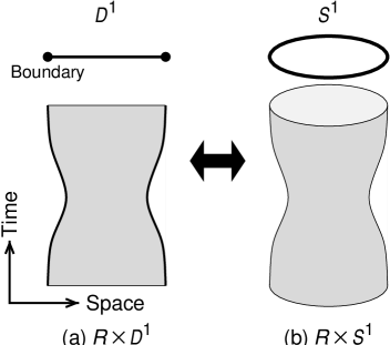
Figure 1: Space times for the $(1+1)$-dimensional Casimir effects. (a) One-dimensional space with two boundaries (one-dimensional disk $D^{1}$) as the cavity between two moving “mirrors.” The scalar field satisfies the fixed boundary condition on the edges. (b) The space $S^{1}$ which is adiabatically equivalent for the scalar field to the geometrical configuration (a). The periodic boundary condition is imposed on the field.

With the help of this replacement, the model in the two-dimensional gravity is applicable to our model. The mirror separation has finite reduced mass $m$ and classically obeys free motion. Then the classical action of our model to describe the system consists of both the classical kinetic term for the scale factor and the Polyakov action,

$$S[D,\phi] \equiv \frac{1}{2\pi}\int dt\frac{m}{2}a^{2}\dot{D}^{2}(t)\;+\;\frac{1}{2}S_{\rm Polyakov}[g_{\mu\nu}(D),\,\phi],$$ (2)

where

$$S_{\rm Polyakov}[g_{\mu\nu},\,\phi] = -\frac{1}{2\pi}\int d^{2}x\>\sqrt{-g}\>\frac{1}{2}\>g^{\mu\nu}\partial_{\mu}\phi\partial_{\nu}\phi.$$ (3)

The Polyakov action is invariant under both the general coordinate transformation and the Weyl transformation. This property is referred to as the conformal symmetry. We can always rewrite the metric into the conformal flat form by the general coordinate transformation:

$$ds^{2} = -dt^{2}+D^{2}(t)dx^{2}\;=\;-C(\eta)\left(d\eta^{2}-dx^{2}\right)\;=\;g_{\mu\nu}\;dx^{\mu}dx^{\nu},$$ (4)

where we have introduced a new coordinate $\eta$ such that $d\eta\equiv dt/D(t)$ and $C(\eta)\equiv D^{2}[t(\eta)]$. After performing the Weyl transformation $g_{\mu\nu}\to C^{-1}(\eta)g_{\mu\nu}$, we have the $D(t)$-independent flat metric,

$$ds^{2} = -d\eta^{2}+dx^{2}\;=\;\eta_{\mu\nu}\;dx^{\mu}dx^{\nu}.$$ (5)

This implies that any deformation of the space size does not affect the classical action. But once we quantize the scalar field, the conformal anomaly appears in general. The quantum effects lead to the motion of the scale factor, i.e., the motion of the mirror separation.

We use a path-integral formulation to evaluate the motion of $D(t)$ as the back reaction of the Casimir effects. We use the background field method, in which the metric is treated as a classical field and the scalar field is quantized. We obtain the effective action for $D(t)$ by integrating out the scalar field. The effective action for the metric, $S_{\rm eff}[D]$, is given by

$$e^{iS_{\rm eff}[D]} \equiv \int{\cal D}\phi\;e^{iS[D,\,\phi]}$$ (6)

$$= e^{i\frac{1}{2\pi}\int dt\frac{m}{2}a^{2}\dot{D}^{2}(t)\;+\;i\frac{1}{2}\Gamma[g_{\mu\nu}(D)]},$$ (7)

$$e^{i\Gamma[g_{\mu\nu}]} \equiv \int{\cal D}\phi\;e^{iS_{\rm Polyakov}[g_{\mu\nu},\,\phi]}.$$ (8)

In order to calculate the effective action for the evolving metric (4), we perform the conformal transformation on the effective action (8) from the evolving metric (4) to the flat metric (5): $g_{\mu\nu}\to e^{2\alpha}g_{\mu\nu}=C^{-1}(\eta)g_{\mu\nu}=\eta_{\mu\nu}$. By means of the Fujikawa method [13] this conformal transformation picks up the conformal anomaly as a Jacobian factor from the path-integral measure in the effective action (8):

$$e^{i\Gamma[g_{\mu\nu}]} = \exp\left[-\frac{i}{2}\int d^{2}x\,\alpha(x)\sum_{n}\varphi^{{\dagger}}_{n}(x)\,\varphi_{n}(x)\right]e^{i\Gamma[\eta_{\mu\nu}]}\quad,$$ (9)

where the parameter of the conformal transformation $\alpha(x)$ is chosen as $\alpha(x)=-\frac{1}{2}\ln C(\eta)$. $\{\varphi_{n}(x)\}$ is a complete set which consists of the eigenfunctions of the Hamiltonian (see Appendix A). The first exponential factor in Eq. (9) is the conformal anomaly, and the second factor is the partition function for the free scalar field in the space $S^{1}$.

3 CASIMIR ENERGY IN SPACE $S^{1}$

We will see that $\Gamma[\eta_{\mu\nu}]$ induces the Casimir energy as the vacuum energy by evaluating the partition function for the free scalar field. Let us calculate the Euclidean partition function

$$Z_{E} \equiv e^{-\Gamma_{E}[\eta_{\mu\nu}]}\;=\;\int{\cal D}{\phi}\,\exp\left[-\frac{1}{2\pi}\int_{-\infty}^{\infty}dx^{2}\int_{0}^{a}dx^{1}\frac{1}{2}\,\partial\phi\,\partial\phi\right],$$ (10)

where we have defined the imaginary time variable $x^{2}\equiv i\eta$, and have used the Euclidean inner product $\partial\phi\partial\phi\equiv\delta^{\mu\nu}\partial_{\mu}\phi\partial_{\nu}\phi$. Since the free Lagrangian is quadratic in terms of $\phi$, this integration can be performed formally, and obtains

$$\ln Z_{E} = -\frac{1}{2}{\rm Tr}\ln(\partial^{2})\;=\;-\frac{1}{2}\int d^{2}x\;\langle x|\ln\partial^{2}|x\rangle.$$ (11)

In the momentum representation the spatial component of the momentum is discretized in the form $(2\pi n/a)$ for arbitrary integers $n$ due to the compactness of the space,

$$\ln Z_{E} = -\frac{1}{2}\,\frac{1}{(2\pi)^{2}}\int d^{2}x\int\frac{dk}{2\pi}\,\frac{1}{a}\,\sum_{n}\;\ln\left[k^{2}+\left(2\pi n/a\right)^{2}\,\right]\;\equiv\;-\frac{1}{(2\pi)^{2}}\int d^{2}xf_{{\rm bare}},$$ (12)

where $f_{{\rm bare}}$ is a bare Euclidean free-energy density for the massless field. Since the integration over $k$ makes $f_{{\rm bare}}$ divergent, we introduce mass $M$ of the scalar field to regularize $f_{{\rm bare}}$ [14], then the integrand is changed as

$$\ln\left[k^{2}\>+\>\left(2\pi n/a\right)^{2}\,\right] \to \ln\left[k^{2}\>+\>\left(2\pi n/a\right)^{2}\>+\>M^{2}\right].$$ (13)

Employing the indefinite integral of $M$, we can write

$$f_{{\rm bare}} = \frac{1}{2}\int\frac{dk}{2\pi}\frac{1}{a}\int dM^{2}\sum_{n}\frac{1}{k^{2}+\left(2\pi n/a\right)^{2}+M^{2}}.$$ (14)

The sum over $n$ can be performed in the expression

$$f_{{\rm bare}} = \frac{1}{2}\int\frac{dk}{2\pi}\int d\omega_{k}\left(1+2\sum_{n=1}^{\infty}e^{-na\omega_{k}}\right),$$ (15)

where we have employed $k$ and $\omega_{k}\equiv\sqrt{k^{2}+M^{2}}$ as independent parameters instead of using $k$ and $M$, and have used the identity

$$\sum_{n=-\infty}^{\infty}\frac{1}{n^{2}+b^{2}} = \frac{\pi}{b}\coth\pi b\;=\;\frac{\pi}{b}\>\left[1+\frac{2}{e^{2\pi b}-1}\right]\;=\;\frac{\pi}{b}\>\left[1+2\sum_{n=1}^{\infty}e^{-2\pi nb}\right].$$ (16)

Since the first term of Eq. (15) indicates the contribution of infinite volume of space time and clearly diverges, we renormalize it as a cosmological term. The second term is relevant for the free-energy density, namely, renormalized free-energy density,

$$f_{{\rm reno}} \equiv -\frac{1}{a}\int\frac{dk}{2\pi}\>\sum_{n=1}^{\infty}\>\frac{1}{n}\>e^{-na\omega_{k}}.$$ (17)

With the identity

$$e^{-na\omega_{k}} = \frac{1}{\sqrt{\pi}}\int_{0}^{\infty}dt\;t^{-1/2}\exp\left[-t-\frac{\left(na\omega_{k}\right)^{2}}{4t}\right],$$ (18)

we perform the integration over $k$, and obtain

$$f_{{\rm reno}} = -\frac{M}{\pi a}\>\sum_{n=1}^{\infty}\>\frac{1}{n}K_{-1}(naM).$$ (19)

Here $K_{\nu}(z)$ is the modified Bessel function

$$K_{\nu}(z) = \frac{1}{2}\left(\frac{z}{2}\right)^{\nu}\int_{0}^{\infty}\frac{dt}{t^{\nu+1}}\exp\left[-t-\frac{z^{2}}{4t}\right].$$ (20)

The free-energy density for the massless field is obtained by taking the limit $M\to 0$. In this limit we can use the property of the Bessel function, $K_{-1}(z)\approx 1/z$ for small $z$, and the free-energy density (19) becomes

$$f_{{\rm reno}} = -\frac{1}{\pi a^{2}}\sum_{n=1}^{\infty}\frac{1}{n^{2}}\;=\;-\frac{\pi}{6a^{2}}.$$ (21)

The Euclidean partition function is derived by substituting Eq. (21) into Eq. (12). After performing the spatial integration, and going back to the Minkowski space with $x^{2}=i\eta$, we obtain

$$\Gamma[\eta_{\mu\nu}] = \frac{1}{i}\ln Z\;=\;\frac{1}{2\pi}\int_{-\infty}^{\infty}dt\;\frac{1}{12}\frac{1}{aD(t)},$$ (22)

where we have used the relation $d\eta=dt/D(t)$. It should be noticed that $-1/(12aD)$ is the Casimir energy in $1+1$ dimensions, and is caused not by the existence of the boundary but by the compactness of the space.

4 CONFORMAL ANOMALY IN SPACE-TIME $R\times S^{1}$

In this section the effective action for the metric $\Gamma[g_{\mu\nu}]$ is derived by evaluating the conformal anomaly in the space-time $R\times S^{1}$. The conformal anomaly is formally expressed by the first exponent in the right-hand side of Eq. (9). This anomaly part appears when the space-size $S^{1}$ is varying with time. Then the anomaly part is considered to describe the back-reactional terms of the dynamical Casimir effect. In the Euclidean space time with the metric $ds^{2}=\rho(x^{2})\>\left[\left(dx^{1}\right)^{2}+\left(dx^{2}\right)^{2}\right]$ the Jacobian induced from the conformal transformation $g_{\mu\nu}\to e^{2\alpha}g_{\mu\nu}$ is

$$J_{E} \equiv \exp\left[-\frac{1}{2}\int_{0}^{a}dx^{1}\int_{-\infty}^{\infty}dx^{2}\,\alpha(x^{2})\sum_{n,k}\varphi^{\dagger}_{n,k}(x)\,\varphi_{n,k}(x)\right],$$ (23)

where $\{\varphi_{n,k}(x)\}$ is a complete set of the eigenfunctions of the Hamiltonian operator,

$$\hat{H} = -\frac{1}{2}\,\frac{1}{\sqrt{\rho}}\,\partial\partial\,\frac{1}{\sqrt{\rho}},\qquad\hat{H}\varphi_{n,k}(x)\;=\;\lambda_{n,k}^{2}\varphi_{n,k}(x).$$ (24)

This Jacobian will be evaluated by using the eigenfunctions $\varphi_{n,k}(x)$ which satisfy the periodic boundary condition in the space $S^{1}$.

The factor $j(x)\equiv\sum_{n,k}\varphi^{\dagger}_{n,k}(x)\varphi_{n,k}(x)$ in the Jacobian (23) has a divergence due to the infinite degrees of freedom of the space-time points. In order to regularize this divergence we introduce a cutoff parameter $M$ and insert the cutoff function $\exp(-\lambda_{n,k}^{2}/M^{2})$ into $j(x)$:

$$j(x)\;\equiv\;\sum_{n,k}\varphi^{{\dagger}}_{n,k}(x)\varphi_{n,k}(x)$$

$$\;\to\; j(x)\;\equiv\;\lim_{M\to\infty}\sum_{n,k}\varphi^{{\dagger}}_{n,k}(x)e^{-\lambda_{n,k}^{2}/M^{2}}\varphi_{n,k}(x)=\lim_{{M\to\infty}}\sum_{n,k}\varphi^{{\dagger}}_{n,k}(x)e^{-\hat{H}/M^{2}}\varphi_{n,k}(x).$$

When we take $\varphi_{n,k}(x)=\frac{1}{\sqrt{a}}e^{ikx^{2}}e^{i(2\pi n/a)x^{1}}$ as the eigenfunction, we obtain

$$j(x)\;=\;\lim_{M\to\infty}\frac{1}{a}\sum_{n=-\infty}^{\infty}\int_{-\infty}^{\infty}\frac{dk}{2\pi}\exp\left[\frac{1}{2M^{2}}\left(-\frac{k^{2}+\left(2\pi n/a\right)^{2}}{\rho}+2\frac{ik}{\sqrt{\rho}}\partial_{2}\frac{1}{\sqrt{\rho}}+\frac{1}{\sqrt{\rho}}\partial_{2}^{2}\frac{1}{\sqrt{\rho}}\right)\right].$$ (25)

Here we should note that $j(x)$ is independent of $x^{1}$. Redefining $k\to Mk$, we can write Eq. (25) with a dimensionless parameter $k$ as

$$j(x^{2}) = \lim_{M\to\infty}\frac{M}{a}\sum_{n=-\infty}^{\infty}\int_{-\infty}^{\infty}\frac{dk}{2\pi}\exp\left[-\frac{{k}^{2}+\left(2\pi n/Ma\right)^{2}}{2\rho}+\frac{i{k}}{M}\frac{1}{\sqrt{\rho}}\partial_{2}\frac{1}{\sqrt{\rho}}+\frac{1}{2M^{2}}\frac{1}{\sqrt{\rho}}\partial_{2}^{2}\frac{1}{\sqrt{\rho}}\right].$$

The second and the third terms in the exponent in Eq. (LABEL:jFunc2.eq) are understood as operators, e.g.,

$$\frac{1}{\sqrt{\rho}}\partial\frac{1}{\sqrt{\rho}} = -\frac{\partial\rho}{2\rho^{2}}+\frac{1}{\rho}\partial.$$ (27)

After expanding the integrand in terms of $M^{-1}$, the order $M^{2}$ terms in Eq. (LABEL:jFunc2.eq) under integrating over $k$ and summation over $n$, denoted as ${\cal O}(M^{2})$, diverge with the limit on $M$. Notice that $\sum_{n=-\infty}^{\infty}\exp\left[-\frac{\left(2\pi n/Ma\right)^{2}}{2\rho}\right]$ gives the contribution of ${\cal O}(M)$. The part of ${\cal O}(M^{2})$, however, is renormalizable by adding a bare cosmological term to the starting Lagrangian [13, 15]. In this expansion the terms in Eq. (LABEL:jFunc2.eq) including only one operator $\frac{i{k}}{M}\frac{1}{\sqrt{\rho}}\partial_{2}\frac{1}{\sqrt{\rho}}$ become ${\cal O}(M)$ because of the existence of the dumping factor, $\exp(-{k}^{2}/2\rho)$. The part of ${\cal O}(M)$ in Eq. (LABEL:jFunc2.eq) becomes zero for symmetric integration on the odd function. Then the next reading terms of ${\cal O}(M^{0})$ in Eq. (LABEL:jFunc2.eq) remain under the limit on $M$. The terms of ${\cal O}(M^{0})$ in Eq. (LABEL:jFunc2.eq) consist of two kinds of contributions. One comes from the operator $\frac{1}{2M^{2}}\frac{1}{\sqrt{\rho}}\partial_{2}^{2}\frac{1}{\sqrt{\rho}}$ in Eq. (LABEL:jFunc2.eq), becoming

$$\frac{1}{Ma}\sum_{n=-\infty}^{\infty}\int_{-\infty}^{\infty}\frac{dk}{2\pi}\;\sum_{m=1}^{\infty}\frac{1}{m!}\left[-\frac{k^{2}+\left(2\pi n/Ma\right)^{2}}{2\rho}\right]^{m-1}$$

$$\qquad\qquad\times\left\{\left(\frac{m^{3}}{6}+\frac{m^{2}}{4}-\frac{m}{24}\right)\rho^{-3}(\partial_{2}\rho)^{2}-\frac{m^{2}}{4}\rho^{-2}\partial_{2}^{2}\rho\right\},$$

and another comes from the two operators of $\frac{i{k}}{M}\frac{1}{\sqrt{\rho}}\partial_{2}\frac{1}{\sqrt{\rho}}$, being

$$\frac{1}{Ma}\sum_{n=-\infty}^{\infty}\int_{-\infty}^{\infty}\frac{dk}{2\pi}\;\sum_{m=1}^{\infty}\frac{(ik)^{2}}{m!}\left[-\frac{k^{2}+\left(2\pi n/Ma\right)^{2}}{2\rho}\right]^{m-2}$$

$$\qquad\qquad\times\left\{\left(\frac{m^{4}}{8}-\frac{m^{2}}{4}+\frac{m}{8}\right)\rho^{-4}(\partial_{2}\rho)^{2}-\left(\frac{m^{3}}{6}-\frac{m^{2}}{4}+\frac{m}{12}\right)\rho^{-3}\partial_{2}^{2}\rho\right\}.$$

After performing the integration over $k$, $j(x^{2})$ becomes

$$j(x^{2}) = \lim_{M\to\infty}\left[F(\rho)\left(\partial_{2}\rho\right)^{2}+G(\rho)\partial_{2}^{2}\rho\right],$$ (28)

where $F(\rho)$ and $G(\rho)$ are given by

$$F(\rho) \equiv \frac{\rho^{-5/2}}{\sqrt{2\pi}Ma}\sum_{n=-\infty}^{\infty}\exp\left[-\frac{1}{2}\left(\frac{2\pi n}{Ma\sqrt{\rho}}\right)^{2}\right]\left\{\frac{5}{32}-\frac{5}{48}\left(\frac{2\pi n}{Ma\sqrt{\rho}}\right)^{2}+\frac{1}{96}\left(\frac{2\pi n}{Ma\sqrt{\rho}}\right)^{4}\right\},$$

$$G(\rho) \equiv \frac{\rho^{-3/2}}{\sqrt{2\pi}Ma}\sum_{n=-\infty}^{\infty}\exp\left[-\frac{1}{2}\left(\frac{2\pi n}{Ma\sqrt{\rho}}\right)^{2}\right]\left\{-\frac{1}{8}+\frac{1}{24}\left(\frac{2\pi n}{Ma\sqrt{\rho}}\right)^{2}\right\}.$$

Under the limit on $M$ we obtain

$$\lim_{M\to\infty}F(\rho) = \frac{\rho^{-2}}{2\pi}\frac{1}{12},\qquad\lim_{M\to\infty}G(\rho)\;=\;-\frac{\rho^{-1}}{2\pi}\frac{1}{12},$$ (29)

with the help of the definition of the Jacobi $\theta$ function and its property:

$$\theta(u,\tau) \equiv \sum_{l=-\infty}^{+\infty}\exp\left(2\pi iul+i\pi\tau l^{2}\right),$$

$$\theta(0,i\tau) \;=\;\frac{1}{\sqrt{\tau}}\>\theta\left(0,\,\frac{i}{\tau}\right).$$

In order to evaluate the effective action (9) with the Euclidean metric $ds^{2}=\rho(x^{2})\>\times\>\left[\left(dx^{1}\right)^{2}+\left(dx^{2}\right)^{2}\right]$, we have to choose the parameter of the conformal transformation as $\alpha(x^{2})=-\frac{1}{2}\ln\rho(x^{2})$. Then the Jacobian factor (23) becomes

$$\ln J_{E}[\rho] = \frac{1}{96\pi}\int_{0}^{a}dx^{1}\,\int_{-\infty}^{\infty}dx^{2}\,\rho^{-2}(\partial_{2}\rho)^{2}.$$ (30)

Now we continue back to the Minkowski Jacobian with time evolving metric (4):

$$\frac{1}{i}\ln J[D] = -\frac{1}{2\pi}\int dt\;\frac{a}{12}\frac{{\dot{D}}^{2}}{D},$$ (31)

where we have used the relations between the Euclidean parameters and the Minkowski ones: $x^{2}=i\eta$, $\rho(x^{2})=C(\eta)$, and we note that $d\eta=dt/D(t),C(\eta)=D(t)^{2},\int dx=a$.

On the other hand, the well-known Polyakov-Liouville action [15], which is the conformal anomaly in the space-time $R^{2}$, brings the same result as Eq. (31), shown as follows. The Polyakov-Liouville action is given by the general form:

$$S_{\rm PL} = -\frac{1}{96\pi}\int d^{2}x\>\sqrt{-g}\>\int d^{2}x^{\prime}\>\sqrt{-g^{\prime}}R(x)\Box^{-1}(x,x^{\prime})\>R(x^{\prime}),$$ (32)

where $R(x)$ is the Ricci curvature. With the form of the metric, $ds^{2}=-C(\eta)\>(d\eta^{2}-dx^{2})$,

$$S_{\rm PL} = -\frac{1}{96\pi}\int_{0}^{a}dx\int d\eta\>C\>\ln C\>\Box\ln C,$$ (33)

and the Ricci curvature is $R(x)=-\Box\ln C$. With the relations, $d\eta=dt/D(t)$ and $C(\eta)=D(t)^{2}$, we come back to the Robertson-Walker-type metric $ds^{2}=-dt^{2}+D(t)^{2}dx^{2}$, and obtain the Ricci curvature in terms of $D(t)$:

$$R(x) = -\Box\ln C\;=\;\frac{2\ddot{D}}{D}.$$ (34)

Here we use $\Box=g^{\mu\nu}\partial_{\mu}\partial_{\nu}=-\frac{1}{C}\partial_{\eta}^{2}$, and the relation $\partial_{\eta}=D\partial_{t}$. By substituting Eq. (34) into Eq. (33), $S_{\rm PL}$ is modified as

$$S_{\rm PL} = \frac{1}{24\pi}\int_{0}^{a}dx\int dt\>\ddot{D}\ln D.$$ (35)

This result is consistent with the well-known fact that the regulated trace of the stress tensor is proportional to the curvature. After the partial integration, Eq. (35) is found to be the same as our result (31), which is the case of $R\times S^{1}$.

Finally, combining the partition function (22) and the Jacobian factor (31) gives the effective action for the space size $D(t)$ as

$$\Gamma[D] \equiv \Gamma[g_{\mu\nu}]\;=\;\frac{1}{i}\ln J+\frac{1}{i}\ln Z\;=\;\frac{1}{2\pi}\int_{-\infty}^{\infty}dt\left(-\frac{1}{12}\frac{\dot{D}^{2}}{D}+\frac{1}{12}\frac{1}{D}\right),$$ (36)

where we have redefined $aD\to D$.

5 BACK REACTION OF THE DYNAMICAL
CASIMIR EFFECT

The semiclassical effective action for the motion of the boundaries is obtained as

$$S_{\rm eff} = \frac{1}{2\pi}\int dt\left(\frac{m}{2}\dot{D}^{2}\;-\;\frac{\kappa}{24}\frac{{\dot{D}}^{2}}{D}\;+\;\frac{\kappa}{24}\frac{1}{D}\right),$$ (37)

where $\kappa$ is the number of species of scalar fields. The second and the third terms come from the effective action (36). In the first term we adopted the same redefinition $aD\to D$ as that in Eq. (36). In this action the second term is the back-reaction term of the dynamical Casimir effect, and the third term is the static Casimir energy. This action leads to the equation of motion given by

$$\left(m-\frac{\kappa}{12}\frac{1}{D}\right)\ddot{D} = -\frac{\kappa}{24}\left(\frac{\dot{D}}{D}\right)^{2}-\frac{\kappa}{24}\frac{1}{D^{2}}.$$ (38)

This equation is integrable, and the resulting relation is given by

$$\left(\frac{m}{2}-\frac{\kappa}{24}\frac{1}{D}\right)\dot{D}^{2}-\frac{\kappa}{24}\frac{1}{D} = E,$$ (39)

where $E$ is an integral constant. The left-hand side is the Hamiltonian of this system, thus $E$ is the energy of this system. Here it should be noticed that the semiclassical condition $m\gg 1/D(t)$ and the adiabatic condition $\dot{D}(t)\ll 1$ lead to the validity condition $|E|\ll m$. Combining the equation of motion (38) and the description of the energy (39), we obtain the mutual dynamical force between the mirrors (boundaries), namely the dynamical Casimir force,

$$F_{\rm dyn}\;\equiv\;m\ddot{D} = -\frac{\kappa}{24}\frac{1}{D^{2}}\;\frac{1+\dot{D}^{2}}{1-\frac{\kappa}{12}\frac{1}{mD}}\;=\;-\frac{\kappa}{24}\frac{1}{D^{2}}\;\frac{1+\frac{2E}{m}}{\left(1-\frac{\kappa}{12}\frac{1}{mD}\right)^{2}}.$$ (40)

The dynamical Casimir force depends on the relative velocity of the mirrors. When the reduced mass $m$ is much larger than the scales $E$ and $1/D$, or equivalently, the velocity $\dot{D}$ is regarded as zero, the dynamical Casimir force (40) is approximately equal to the static one:

$$F_{\rm static}\;\equiv\;-\frac{\partial}{\partial D}\left(-\frac{\kappa}{24}\frac{1}{D}\right) = -\frac{\kappa}{24}\frac{1}{D^{2}}.$$ (41)

The ratio of the dynamical force $F_{\rm dyn}$ to the static one $F_{\rm static}$ is given by

$$F_{\rm dyn}/F_{\rm static} = \frac{1+\dot{D}^{2}}{1-\frac{\kappa}{12}\frac{1}{mD}}\;=\;1\>+\>\frac{\kappa}{12}\frac{1}{mD}\>+\>\dot{D}^{2}\>+\>\cdots.$$ (42)

Here the $\dot{D}^{2}$ term in the expansion is known as the negative-frictional-like-force [8]. Since $\dot{D}^{2}\geq 0$, we conclude that the dynamical force $F_{\rm dyn}$ is always attractive and stronger than the static one $F_{\rm static}$ for $D>\frac{\kappa}{12}\frac{1}{m}$.

6 CONCLUSION AND DISCUSSIONS

In this paper we presented an effective theoretical approach to studying the Casimir effects in $1+1$-dimensions within the adiabatic approximation. The point of our investigation was the replacement of the spatial configuration: $D^{1}\rightarrow S^{1}$. We constructed the effective action of the scalar field model, and checked the validity of this replacement. In our model the quantum correction to the classical kinetic term of the mirror separation was calculated by the path-integral formalism. The resultant quantum correction naturally contains both the ordinary Casimir energy term and the back-reaction term of the dynamical Casimir effect. The semiclassical effective action (37) was constructed of the classical kinetic term of the mirror separation and these resultant quantum corrections. From the action (37), we have obtained the dynamical vacuum pressure. The pressure (dynamical Casimir force) includes the back-reactional force of the dynamical Casimir effect. The dynamical Casimir force was confirmed to be attractive and always stronger than the static Casimir force. The dynamical Casimir force depends on the relative velocity of the mirrors, and it is reduced to the static one when the velocity goes to zero.

The perturbative expansion of the resultant dynamical Casimir force (42) includes the term for the negative frictional force which agrees with the result of Dodonov et al. [8]. Although this means that our result is not entirely new, our approach reproduces the reliable result, thus it can be said that we have presented a unique effective theoretical approach to the problem.

Several easier derivations of the static Casimir energy in the Hamiltonian formulation are known, but our method needs a more complex calculation to obtain the Casimir energy. Our approach, however, describes both the static and the dynamical Casimir effects together, and is applicable to more realistic models in the higher dimensions by replacing the space $D^{1}\times R^{n}$ into $S^{1}\times R^{n}$.

Furthermore, the existence of the action makes it easy for us to compare our model with others. For example, our model has a correspondence to the Callan, Giddings, Harvey, Strominger (CGHS) model which describes the two-dimensional dilaton black hole [16]. The back reaction discussed in this paper is comparable to the back reaction of the Hawking radiation from the CGHS black hole [17]. In the CGHS model the Hawking radiation is represented by the conformal anomaly in the energy-momentum tensor [16], and the back reaction of the radiation, which is described by the Polyakov-Liouville action, appears as the decrease in the black-hole mass [17]. Our classical kinetic term in the semi-classical effective action (37) corresponds to the kinetic term of the dilaton in the CGHS model.

Some comments are in order.

The quantum correction (36) does not include the third derivative of the dynamical variable. This looks different from the results evaluated by Fulling and Davies [6]. They calculated the energy-momentum tensor in (1+1)-dimensional system of two relatively moving mirrors [6] as well as that in (1+1)-dimensional system of a single non-uniformly accelerating mirror [6, 18]. Both energy-momentum tensors include the third derivative of the dynamical variables. Our result for the system of two mirrors does not need to coincide with their result for the system of a single mirror since the forms of the conformal anomaly for two systems are different. The result for the system of a single mirror is due to the Unruh-like effect rather than due to the dynamical Casimir effect. On the other hand, the energy-momentum tensor derived from Eq. (36) coincides with their result for the system of two mirrors under a certain transformation of the dynamical variable.

In the semiclassical effective action (37), the contribution from the dynamical Casimir effect generated a negative-definite kinetic term of the mirror separation. Such a kinetic term also appeared in the analysis of the CGHS model [17]. The following point should be noted: there is a positive-definite classical kinetic term, and the negative-definite term gives only a slight correction. This holds in the case where the mass scale of the mirrors $m$ is much greater than the scale of the Casimir energy $\sim D^{-1}$. On the other hand, if the mirror separation $D(t)$ is smaller than the inverse of the mirror mass $m^{-1}$, our result (40) shows that the dynamical Casimir force $F_{\rm dyn}$ becomes repulsive. However, our semiclassical treatment becomes unsuitable at that time. When the motion of the mirror separation obeys the quantum mechanics, this repulsive force might be realized. We will leave this problem to subsequent developments.

ACKNOWLEDGMENTS

We would like to thank Professor S. Uehara, Professor M. Harada, and Professor A. Nakayama for their useful discussions and suggestions. We thank Professor V. A. Miransky for discussions. We also appreciate helpful comments of Professor A. Sugamoto, Professor H. Funahashi, Dr. T. Itoh, Dr. A. Takamura, Dr. S. Sugimoto, Dr. Y. Ishimoto, and Dr. S. Yamada. We are also grateful to Professor R. Schützhold for his interest in our work and enlightening discussions on related matters. He suggested that no particle creation occurs in our model, and that this work is related to the dynamical back reaction of the static Casimir effect. One of us (Y.N.) is indebted to the Japan Society for the Promotion of Science (JSPS) for its financial support. The work is supported in part by a Grant-in-Aid for Scientific Research from the Ministry of Education, Science and Culture (No. 03665).

APPENDIX A: Fujikawa method

In this appendix we briefly explain the derivation of the expression (9) from the definition of the effective action (8). This derivation is based on the evaluation of the conformal anomaly by the Fujikawa method [13]. In order to perform the path integration of Eq. (8), we make a Wick rotation by introducing an imaginary time variable $x^{2}\equiv i\eta$. Then the Euclidean metric corresponding to the Minkowski one (4) becomes

$$ds^{2} = \rho(x^{2})\>[(dx^{1})^{2}+(dx^{2})^{2}].$$ (A1)

The Euclidean effective action is

$$e^{-\Gamma_{E}[g_{\mu\nu}]} = \int{\cal D}\phi\>\exp\left[-\frac{1}{2\pi}\int d^{2}x\>\sqrt{g}\>\frac{1}{2}\>g^{\mu\nu}\>\partial_{\mu}\phi\>\partial_{\nu}\phi\right].$$ (A2)

By introducing $\tilde{\phi}\equiv\sqrt[4]{g}\>\phi$ and changing the measure ${\cal D}\phi$ into the invariant form under the general coordinate transformation ${\cal D}\tilde{\phi}$, Eq. (A2) becomes

$$e^{-\Gamma_{E}[g_{\mu\nu}]} = \int{\cal D}{\tilde{\phi}}\>\exp\left[-\frac{1}{2\pi}\int d^{2}x\>\frac{1}{2}\partial\left(\frac{\tilde{\phi}}{\sqrt{\rho}}\right)\partial\left(\frac{\tilde{\phi}}{\sqrt{\rho}}\right)\right].$$ (A3)

Here we have used a notation $\partial\phi\,\partial\phi\equiv\partial_{1}\phi\,\partial_{1}\phi+\partial_{2}\phi\,\partial_{2}\phi$. We perform a mode expansion of the field $\tilde{\phi}(x)$ in terms of a complete set $\{\varphi_{n}(x)\}$:

$$\tilde{\phi}(x) = \sum_{n}\>a_{n}\varphi_{n}(x)\;\equiv\;\sum_{n}\>\langle x|n\rangle\>a_{n},$$ (A4)

where we have chosen ${\varphi_{n}(x)}$ as an eigenfunction of the Hamiltonian operator,

$$\hat{H} = -\frac{1}{2}\,\frac{1}{\sqrt{\rho}}\,\partial\partial\,\frac{1}{\sqrt{\rho}},\qquad\hat{H}\varphi_{n}(x)\;=\;\lambda_{n}^{2}\,\varphi_{n}(x).$$ (A5)

Here $\varphi_{n}(x)$ satisfies the normalization $\int d^{2}x\>\varphi^{{\dagger}}_{m}(x)\>\varphi_{n}(x)\>=\>\delta_{mn}$. Now we note that the measure ${\cal D}\tilde{\phi}$ is expressed by the mode coefficients $a_{n}$ as

$${\cal D}\tilde{\phi} = \prod_{x}\>{\cal D}\tilde{\phi}(x)\;=\;\left[\,\det\langle x|n\rangle\,\right]\>\prod_{n}\>da_{n}\;=\;\prod_{n}\>da_{n}.$$ (A6)

Under the Weyl transformation $g_{\mu\nu}\to e^{2\alpha(x)}g_{\mu\nu}$ the mode coefficients of the field $\tilde{\phi}(x)$, $a_{n}$, are transformed as an infinitesimal form,

$$\tilde{\phi}(x) \to \tilde{\phi}^{\prime}(x)\;\equiv\;\sum_{n}\,a^{\prime}_{n}\,\varphi_{n}(x),$$

$$a^{\prime}_{n} = a_{n}\>+\>\sum_{m}\frac{1}{2}\int d^{2}x\>\alpha(x)\varphi^{{\dagger}}_{n}(x)\>\varphi_{m}(x)a_{m}\;\equiv\;\sum_{m}C_{nm}\,a_{m}.$$ (A7)

Then the measure is transformed as

$${\cal D}\tilde{\phi}^{\prime} = \prod_{n}da^{\prime}_{n}\;=\;\left[\det(C_{nm})\right]\>\prod_{l}da_{l}$$ (A8)

$$= \exp\left[{\rm Tr}\ln\left(\delta_{nm}\;+\;\frac{1}{2}\int d^{2}x\>\alpha(x)\varphi^{{\dagger}}_{n}(x)\>\varphi_{m}(x)\right)\right]\;\prod_{l}da_{l}$$

$$= \exp\left[+\frac{1}{2}\int d^{2}x\>\alpha(x)\sum_{n}\varphi^{{\dagger}}_{n}(x)\>\varphi_{n}(x)\right]\;{\cal D}\tilde{\phi}.$$

This gives the Jacobian of the conformal transformation. By the Weyl transformation chosen $\alpha(x)=-\frac{1}{2}\ln\rho(x)$ for $\tilde{\phi}\to\tilde{\phi}^{\prime}=\tilde{\phi}/\sqrt{\rho}$, the effective action (A3) becomes

$$e^{-\Gamma_{E}[g_{\mu\nu}]} = \exp\left[-\frac{1}{2}\int d^{2}x\,\alpha(x)\sum_{n}\varphi^{{\dagger}}_{n}(x)\,\varphi_{n}(x)\right]$$ (A9)

$$\times\int{\cal D}{\tilde{\phi}^{\prime}}\,\exp\left[-\frac{1}{2\pi}\int d^{2}x\,\frac{1}{2}\,\partial\tilde{\phi}^{\prime}\,\partial\tilde{\phi}^{\prime}\right],$$

where the second factor equals to the partition function of the free scalar field in the flat space time. Finally, we can arrive at our destination (9) from the description (A9) by the inverse Wick rotation.

APPENDIX B: Another path-integral Calculation of the Casimir energy

In this appendix we give another partition-functional derivation of the Casimir energy by means of the point-splitting ansatz and the Feynman prescription: In the path-integral method the partition function part in (9) can be also evaluated by using the point-splitting ansatz and the Feynman’s renormalization prescription. Employing the ansatz of point splitting to (10),

$$Z_{E} = \int{\cal D}{\phi}\,\exp\left[-\frac{1}{2\pi}\int d^{2}x\frac{1}{2\pi}\int d^{2}x^{\prime}\frac{1}{2}\phi(x)A(x,x^{\prime})\phi(x^{\prime})\right]$$ (B1)

$$= \exp\left[-\frac{1}{2}{\rm Tr}\ln A\right],$$

where $\int d^{2}x\equiv\int_{-\infty}^{\infty}dx^{2}\int_{0}^{a}dx^{1}$, and $A(x,x^{\prime})\equiv\delta^{\mu\nu}\partial_{\mu}\partial^{\prime}_{\nu}\delta^{(2)}(x-x^{\prime})$. The two-dimensional Dirac delta function in the integral representation is

$$\delta^{(2)}(x-x^{\prime}) = \frac{1}{a}\,\sum_{n=-\infty}^{+\infty}\int\frac{dk}{2\pi}\,e^{-ik(x^{2}-x^{\prime 2})}\,e^{i\frac{2\pi n}{a}(x^{1}-x^{\prime 1})}\;.$$ (B2)

Now we come back to Minkowski space and introduce mass $M$ of the scalar field to regularize the integral,

$$\frac{1}{i}\ln Z = -\frac{1}{2}\,\frac{1}{(2\pi)^{2}}\int d^{2}x\int d^{2}x^{\prime}\,\delta^{(2)}(x-x^{\prime})\,\frac{1}{a}\,\sum_{n}\,e^{i\frac{2\pi n}{a}(x-x^{\prime})}$$ (B3)

$$\times\;\int dM^{2}\int\frac{dk}{2\pi}\,\frac{e^{-ik(\eta-\eta^{\prime})}}{-k^{2}+\left(2\pi n/a\right)^{2}+M^{2}}\;.$$

With the $i\epsilon$ prescription, we perform the integral in the complex $k$ plane, applying the residue theorem,

$$\int\frac{dk}{2\pi}\,\frac{e^{-ik(\eta-\eta^{\prime})}}{-k^{2}+\left(2\pi n/a\right)^{2}+M^{2}-i\epsilon}$$

$$=\theta(\eta-\eta^{\prime})\frac{i}{2\sqrt{\left(2\pi n/a\right)^{2}+M^{2}}}+\theta(\eta^{\prime}-\eta)\frac{-i}{-2\sqrt{\left(2\pi n/a\right)^{2}+M^{2}}},$$ (B4)

where $\epsilon>0$ and $\theta(x)$ is the step function. Here we define the new parameter, $\omega_{n}^{2}\equiv\left(2\pi n/a\right)^{2}+M^{2}$, and replace the integral into the following form:

$$\int dM^{2}\,\frac{1}{2\sqrt{\left(2\pi n/a\right)^{2}+M^{2}}} = \int d\omega_{n}\;=\;\omega_{n}.$$ (B5)

Then we take the massless limit $M\to 0$ and perform the summation,

$$\sum_{n=-\infty}^{+\infty}\omega_{n} = \frac{4\pi}{a}\sum_{n=1}^{\infty}n\;=\;\frac{4\pi}{a}\zeta(-1)\;=\;-\frac{\pi}{3a}.$$ (B6)

At last we arrive at the same form of Eq. (22),

$$\frac{1}{i}\ln Z\;=\;\frac{1}{2\pi}\int_{-\infty}^{\infty}dt\;\frac{1}{12}\frac{1}{aD(t)}.$$ (B7)

References

- [1] H. B. G. Casimir, Proc. K. Ned. Akad. Wet. 51, 793 (1948).
- [2] T. H. Boyer, Phys. Rev. 174, 1764 (1968).
- [3] M. J. Sparnaay, Physica (Utrecht) 24, 751 (1958).
- [4] S. K. Lamoreaux, Phys. Rev. Lett. 78, 5 (1997); U. Mohideen and A. Roy, Phys. Rev. Lett. 81, 4549 (1998).
- [5] G. T. Moore, J. Math. Phys. 11, 2679 (1970).
- [6] S. A. Fulling and P. C. W. Davies, Proc. R. Soc. London, Ser A 348, 393 (1976).
- [7] E. Sassaroli, Y. N. Srivastava, and A. Widom, Phys. Rev. A 50, 1027 (1994).
- [8] V. V. Dodonov, A. B. Klimov, and V. I. Man’ko, Phys. Lett. A 142, 511 (1989).
- [9] M. Castagnino and R. Ferraro, Ann. Phys. (N.Y.) 154, 1 (1984); G. Calucci, J. Phys. A 25, 3873 (1992); C. K. Law, Phys. Rev. Lett. 73, 1931 (1994); V. V. Dodonov, Phys. Lett. A 207, 126 (1995); O. Méplan and C. Gignoux, Phys. Rev. Lett. 76, 408 (1996); A. Lambrecht, M. T. Jaekel, and S. Reynaud, Phys. Rev. Lett. 77, 615 (1996); J. Y. Ji, H. H. Jung, J. W. Park, and K. S. Soh, Phys. Rev. A 56, 4440 (1997); D. A. R. Dalvit and F. D. Mazzitelli, Phys. Rev. A 57, 2113 (1998); 59, 3049 (1999); R. Golestanian and M. Kardar, Phys. Rev. A 58, 1713 (1998).
- [10] L. Parker, Phys. Rev. 183, 1057 (1969); Ya. B. Zel’dovich, Zh. Éksp. Teor. Fiz. Pis’ma. Red. 12, 443 (1970); [JETP Lett. 12, 307 (1970)]; W. G. Unruh, Phys. Rev. D 10, 3194 (1974).
- [11] S. W. Hawking, Commun. Math. Phys. 43, 199 (1975).
- [12] P. Davies, Nature (London) 382, 761 (1996).
- [13] K. Fujikawa, Phys. Rev. D 25, 2584 (1982).
- [14] A. K. Ganguly and P. B. Pal, e-print hep-th/9803009.
- [15] A. M. Polyakov, Phys. Lett. 103B, 207 (1981).
- [16] C. G. Callan, S. B. Giddings, J. A. Harvey, and A. Strominger, Phys. Rev. D 45, 1005 (1992).
- [17] J. G. Russo, L. Susskind, and L. Thorlacius, Phys. Lett. B 292, 13 (1992).
- [18] N. D. Birrell and P. C. W. Davies, Quantum Fields in Curved Space (Cambridge University Press, London, 1982).