Universality and conformal invariance
for the Ising model in domains with boundary
Abstract
The partition function with boundary conditions for various two-dimensional Ising models is examined and previously unobserved properties of conformal invariance and universality are established numerically.
Keywords: Ising model, boundary conditions, renormalization group, free boson, conformal invariance, critical phenomena.
1 Introduction.
Although the experiments of this paper, statistical and numerical, were undertaken in pursuit of a goal not widely shared, they may be of general interest since they reveal a number of curious properties of the two-dimensional Ising model that had not been previously observed.
The goal is not difficult to state. Although planar lattice models of statistical mechanics are in many respects well understood physically, their mathematical investigation lags far behind. Since these models are purely mathematical, this is regrettable. It seems to us that the problem is not simply to introduce mathematical standards into arguments otherwise well understood; rather the statistical-mechanical consequences of the notion of renormalization remain obscure.
Our experiments were undertaken to support the view that the fixed point (or points) of the renormalization procedure can be realized as concrete mathematical objects and that a first step in any attempt to come to terms with renormalization is to understand what they are. We have resorted to numerical studies because a frontal mathematical attack without any clear notion of the possible conclusions has little chance of success. We are dealing with a domain in which the techniques remain to be developed.
A fixed point is a point in a space of presumably an infinite number of dimensions; so this point and all other points of the space are defined by an infinite number of coordinates. Some will presumably be superfluous, so that the total space is realized as a submanifold of some larger coordinate space. The total space will be the carrier, in some sense, of the renormalization transformation, but the transformation will not appear explicitly in this paper. The point does! The implicit condition on each quantity serving as a possible coordinate of the fixed point is that, at the fixed point itself, it remains invariant under renormalization and that, at a critical point of any model within the class considered, its value approaches a limit under repeated renormalization because renormalization drives the critical point to the fixed point. Since repeated renormalization is in coarsest terms nothing more than passage to larger and larger blocks or to smaller and smaller mesh, the condition is that the quantity has a meaning as the mesh length goes to zero, the dimensions otherwise remaining the same. For percolation this is a property of crossing probabilities. Our point of view is that any such quantity is a candidate as a possible coordinate in the space of the fixed point. Rather than a single numerical quantity we can consider several at once, which amounts in the customary mathematical way to considering objects lying in some given space, finite-dimensional or infinite-dimensional, for example, a space of probability distributions, and if these objects satisfy this criterion, thus if, for each model at the critical point, they tend to a limit as the mesh goes to zero, then this limit or rather its coordinates in the given space can also serve as coordinates of the fixed point. Such objects are described in the paper.
There are at least two possibilities: one modeled on the considerations for the free boson of [L]; the other on the crossing probabilities for percolation [LPPS, LPS]. The second possibility was suggested to us by Haru Pinson to whom we are grateful. Thus to each form of the Ising model (taken at the critical temperature) we will attach two points and , each defined by an infinite number of coordinates. Both are, in so far as this can be confirmed by experiments, universal and conformally invariant in the sense of [LPS]. It is unlikely that these two points are independent. One set of coordinates may well be deducible from another, but we have not examined this possibility.
Crossing probabilities may or may not be peculiar to a few models. The evidence for their conformal invariance and universality is not difficult to present and appears in Section 5. There is, however, one point to underline. The Ising model is considered in regions that may be bounded or unbounded. Crossing probabilities are defined for crossings within a region that may or may not coincide with the region in which the model is considered. It may be smaller. In contrast to crossing probabilities for percolation, in which there is no interaction, those for the Ising model depend on both the region in which the crossings are allowed to occur and the region of thermalization on which the Ising model is considered. Conformal invariance refers to the simultaneous action of a conformal mapping on the pair of regions.
The coordinates modeled on the free boson should, on the other hand, be available for a large class of models. Their definition is, in principle, quite general, but we have confined ourselves to the Ising model. The states of the Ising model take values in the set which is contained in the set of all complex numbers with . This set in turn is covered by the line . We simply develop the circle on the line. We first assign to one site in the lattice the value and then choose for all other the value , , so that . Of course, there has to be more method than that. For example, for the square lattice we introduce clusters: maximal collections of lattice sites of the same spin that are connected through bonds joining nearest-neighbor sites. Each cluster is surrounded by a curve constructed from edges of the dual lattice and this curve separates it from all other clusters. To each of these curves an orientation is assigned randomly and, for nearest neighbors and , we set , the sign being determined by the relative orientation of the bond from to and the curve it crosses. If it crosses no curve, then and we take . Thus to every state are attached several functions , but determines up to sign. For a finite lattice the measure on , the set of all possible is taken to be such that the measure, , on assigns the same mass to all points lying above a given . Their sum is one-half the mass of .
Fix now a bounded planar region and consider the Ising model in this region with respect to a square lattice whose mesh approaches . Since the model is to be critical, the contribution to the Boltzmann weight of a pair of neighboring spins is
Each is in effect a function on the whole region if we take the value in the open square of side about the site to be . (The ambiguity at the boundary is disregarded here; it has to be confronted in various ways from experiment to experiment.) If is a (smooth) curve in , which can lie entirely in the interior or run entirely or partially along the boundary, then we can restrict each function in to . This yields a set of points, each carrying a mass, in the set of Schwartz distributions on , and thus a probability measure on . Experiments to be described in Sections 2 and 3 suggest strongly that this measure has a limit as the mesh tends to and that the limit is universal and conformally invariant. This is perhaps the most important conclusion of the paper.
These measures have surprised the authors more than once. When is the boundary, the measure has a number of properties, to which we devote considerable attention, that suggest it is gaussian. It is not.
There is no reason to restrict ourselves to planar regions and we begin our study with the cylinder, because the ambiguities at the boundary are then absent. A long cylinder (effectively semi-infinite) is, provided we stay close to the end, to be regarded as equivalent to a disk. The simplest conformally invariant distribution on the set of distributions on the boundary of a disk is the gaussian distribution with respect to the quadratic form defined by the Dirichlet form. For a function this form is obtained by extending to a harmonic function in the interior and then taking
| (1) |
The first experiments described in Section 2 strongly suggest that the measure given by our construction is in some respects very similar to this gaussian with a constant that appears to be universal; the final experiments of that section show, however, that it differs in important respects from a gaussian. If is interior, the measure on is in no respect similar to a gaussian.
Our construction is different from but not unrelated to familiar constructions relating the Ising model to SOS models. For the Ising model on a triangular lattice our construction is equivalent in many respects to the usual one for the -model. In particular, it is expected that in the plane
The constant is expected to be , at least for the triangular lattice, but the two constants and are not equal.
Although is usually defined only for the triangular lattice, it can be defined in general. We suppose that it is universal, but we have not examined this carefully. The pertinent experiments are briefly discussed in Section 6. The conclusion, which will be reinforced more than once as we proceed, is that the comparison with the free boson undertaken in this paper is quite different than the usual one.
There is no reason that the two constants and should be equal. One refers to interior behavior in the bulk, the other to behavior on the boundary. Moreover, as it turns out, they refer to different aspects of a construction that leads to nongaussian measures with some gaussian behavior. Although a departure from the conventional view, it could be argued (we do not attempt to do so here) that for questions of renormalization the constant may be every bit as important as , or, much better, that the distributions on curves of Section 2 are at least as important for renormalization as asymptotic behavior because renormalization, at least as it is often presented, entails the fusion of bounded regions along their boundaries (which may or may not partially coincide with that of the region of thermalization). The measures on were originally examined only for curves on or close to the boundary. They appear, somewhat to our surprise, to be of interest even in the absence of a boundary. Indeed it may turn out, with hindsight, that the numerical arguments towards the end of Paragraph 3.2 for the existence of nontrivial and conformally invariant measures on interior curves are at least as important as the other results, argued more elaborately and with more detail, of Sections 2 and 3.
Our point of view would not be at all persuasive if there were no sign in our fixed point , thus in the measures on , of the critical indices , and . It is seen in Paragraphs 2.3 and 3.2 that these measures do contain information about critical indices. Section 4, in which we describe another manifestation of the index as well as an interpolation of a formula of Cardy, is also an essential part of the paper.
The final section is less important. It contains a few observations that provide some perspective on the definitions of the paper. First of all, the construction of is by no means canonical. There are alternative constructions decribed in Section 7. We can allow jumps other than , in particular several jumps , odd, with equal or different probabilities. They lead to different values of and to a measure on with little resemblance to a gaussian.
The possibility of not using clusters in our sense but the clusters of Fortuin and Kasteleyn that appear in the high-temperature expansion of the Ising (or more generally the Potts) model also suggests itself. Such clusters can also be used to define the crossing probabilities. They lead to different measures and to different crossing probabilities, whose universality and conformal invariance we have not tested.
Finally we point out that the results for the distributions appear to remain valid at infinite temperature with, of course, a different value for the parameter appearing in the distribution.
We are grateful to Michael Aizenman, Christian Mercat, Haru Pinson and Thomas Spencer for observations and suggestions that have been useful to us during the course of these investigations.222RPL is grateful to Alois Scharf for making the bank of computers of the Mathematisches Institut der Universität Bonn available to him at an important moment in the experimentation. Our most important debt is to the statistician Christian Léger whose counsel and advice were of enormous help in the preparation of Section 2.
Questions and comments of the referee, to which in particular the discussion relating statistical dependence and the two-point correlation function in Paragraph 2.3 is a response, led to at least one important modification of the conclusions in the original version of the paper.
2 Distribution of at the boundary.
2.1 The free boson on domains with boundary conditions.
The partition functions of a free boson , with compactification radius , are familiar objects when the domain is a torus, or a rectangle with the field satisfying Dirichlet boundary conditions, thus equal to on the boundary. For a general Riemann surface with boundary and for an arbitrary specification of the field at the boundary, it may still be possible to describe the partition functions explicitly (see [CG]). For a cylinder we use the formula of [L]. As it suggested some of the statistical quantities for the Ising model studied in this paper, we review this formula.
The cylinder is described as the quotient of the region , , in the complex plane by the transformations generated by , . If the fundamental domain is chosen to be and , the map identifies the cylinder with the annulus of outer radius and inner radius . We shall use freely the terminologies associated with the cylinder and with the annulus. Observe that is close to zero for long cylinders. The angle is used as the parameter on both the inner and the outer boundary.
The extremal fields on the domain are real harmonic functions
The boundary conditions fix the restriction of to the boundary. On the inner circle where and , this restriction is
with the reality condition and on the outer circle
with . (The superscript stands for boson.) The compactification condition does not require to be periodic but imposes a milder condition: , thus . Since the Lagrangian function (1) does not depend on the term , this constant can be set to zero. Therefore only the difference of the constant terms in and is of significance and we choose to parametrize it with a variable and an integer :
| (2) |
The partition function on the cylinder with the boundary values of specified by , , or equivalently by and , is a product of three terms [L]
| (3) | ||||
| (4) |
where is the -regularization of the determinant of the Laplacian for the annulus. It is given by where and is the Dedekind function. Since this factor is independent of the boundary data, it will be disregarded. The crucial terms here are the two other factors
| (5) |
and
| (6) |
If measurements are made disregarding the variable , only
is of importance and this gives, after proper normalization, a probabilistic measure on the space of boundary data parametrized by . The mixing of the boundary data at both extremities becomes more and more intricate when approaches or, in other words, when the cylinder becomes a narrow ring. When is taken to zero, the measure simplifies as it becomes the product of two terms, each one depending on or . Moreover, in the limit , the probabilistic interpretation of is simply that of the gaussian measure in the variables and .
Even though the Coulomb gas provides a description of the minimal models, we do not know of any similar explicit formula for the partition functions of these models for general boundary conditions, although Cardy’s paper [C1] treats explicitly the case of conformally invariant boundary conditions. There are indeed only a finite number of these, and one of the difficulties addressed in this paper is how to introduce continuously varying conditions. Nonetheless we proceed boldly using the partition function (4) as a guide for the Ising model. In contrast to the free-boson model, the Ising model defined on a graph does not have a field taking its values in the whole real line that we could easily identify with – the spin field takes its values in . Starting from the spin field , defined on the sites of a (finite) graph , one can construct the function as described in the introduction. It is such that, if and are joined, then if and otherwise. If the graph is embedded in a surface , for example, a cylinder or , this function can be extended to a function locally constant on except on the edges of the dual graph where it has jumps. The Ising measure on the space of configurations on the graph of mesh endows the (finite) set of possible functions with a (discrete) probability measure. (As observed above, this measure is such that where is the number of distinct ’s that lead to and .)
Take the graph to be the subset of the lattice of mesh formed by the points , , . We identify upper and lower edges and regard the graph as a subset of the cylinder: . How can we compare to the field-theoretic measure of the free boson? Using the same letters and (but without the superscript “”) for the Fourier coefficients of the restriction of to the extremities of a cylinder:
we study the dependence upon and , of the measure on , disregarding all other coefficients. The object obtained this way is a measure on concentrated on a finite set. Keeping fixed, we then take the mesh on to zero. If the limit of the measures on exists, presumably as a continuous distribution, the limit as the number of Fourier coefficients is taken to infinity can be considered. We name the limiting object
| (7) |
This measure, if it exists, is therefore defined on a space with coordinates and we shall denote the elements of this space by . This measure is to be compared with the probability measure induced by (4) on the space of . (The radius of compactification appears here because we normalized the jumps of the function to be , forcing to change by an integral multiple of as winds around one extremity.) The first, and principal, question is:
-
(i)
does the measure exist?
The parallel just suggested can be pushed further. We introduce first the derivative of the restriction of to either extremity. It is clearly a sum of delta functions concentrated half way between those sites and at the boundary such that . The mass of each jump is . We shall use the letter for its Fourier coefficients,
Clearly . At the other end we use . We will use equally for the coordinates parametrizing , the derivative . For the boson, the probabilistic interpretation of the partition function implies that the -th Fourier coefficient of the restriction is distributed (up to a normalizing factor) as in the limit . Consequently, if we use the Fourier coefficients of
with , the probability density is , again up to normalization. For a long cylinder the parallel drawn here raises the following questions on granted, of course, that the answer to (i) is positive:
-
(ii)
are the random variables defined by the Fourier coefficients of distributed normally as ?
-
(iii)
is there a constant such that the constants are simply related by
(8) -
(iv)
is the joint distribution a product of independent single-variable distributions?
The rest of this section will describe the response to these questions provided by numerical simulations. The next will provide evidence that this limit measure is both universal and conformally invariant.
2.2 The distribution of at the boundary of a long cylinder.
The diagrams of Figure 1 are some evidence for the existence of the distribution on the space . They represent the probability distribution densities of restricted to one of the extremities of various cylinders, in terms of a single variable (either or ), all others being disregarded or, thinking in terms of the limit, integrated out. By rotational symmetry these densities are (almost) identical to those with respect to the imaginary part of the same coefficients. (A small discrepancy could arise from the fact that the numbers of sites along the circumference were not divisible by 4.) The square lattices contained , , , , and sites. The first number () is the number of sites around the circumference and is half the number of sites along the length () minus one, or less. The Appendix gives some further technical details on the simulations. We note at this point that the partition function (4) is obtained by summing over the integer parametrizing the linear term in both and . The analogue of this term for Ising configurations is straightforward: a configuration with exactly two clusters (of opposite signs) extending from one end to the other of the cylinder will have two longitudinal jump lines. Depending on the choice of the jump across these lines, will increase by and as wraps around the boundary. Other (even) integral multiples of appear for configurations with more clusters crossing from one end to the other and the numbers can be used to partition the set of configurations. We have not differentiated the measure for these various classes. We should add that, for the cylinders studied in the present section, the configurations whose linear term is zero are by far the most probable. The multiples occurred with a probability about ; higher multiples we did not see at all.
Even though the raw data clearly differentiate the curves attached to smaller cylinders, smoothing helped to separate the curves between the two largest one ( and ). This smoothing was done using the kernel method with a gaussian kernel; the smoothing parameter was chosen according to Eq. (3.28) of [Si], in which was taken to be the sample standard deviation.
The narrowing of the gaps between the curves as the number of sites is increased is a good qualitative argument for the existence of the limit . The peaks of the curves go down systematically as and increase, except for the dependence on . In this case the center of the curve for lies slightly above the center for on the small interval . Around the two curves cross and the curve for remains below that for until approximately . From then on () the two curves are so close that they cross each other several times, probably due to the limitation of our samples. This puzzled us and was checked independently by two of us. We have no explanation for it. As will be seen below however, the variance of the samples, a more global indicator, increases systematically over the spectrum of all the cylinders considered; in particular that of is larger than that of .
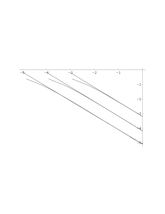
These distribution densities are so similar to normal curves that their variances are a natural tool for a more qualitative assessment of the finite size effects. In order to answer questions (ii) and (iii), we plot in Figure 2 the numbers
where is the square root of the variance with respect to the variable for the cylinder with sites. (If both questions were to be answered positively, then the numbers for would be a constant. Note that we follow the usual statistical convention of distinguishing between the theoretical value of a quantity and its measured value .) We plotted these numbers for (or, sometimes, ), together with a linear fit of these ten points for every cylinder size on the square lattice considered, the largest triangular and hexagonal lattices, the anisotropic lattice, and the square and disk geometries. The latter will be discussed in in Section 3. The data, read from the top, appear in the order: cylinders of size , , , for the square lattice ; of size for the hexagonal lattice ; then of size for ; of size for the anisotropic lattice; of size for the triangular lattice ; the cylinder of size for and the square of size are superimposed; and finally the disk of radius for . The numerical data are also recorded in Table I for together with those for triangular and hexagonal lattices on a cylinder and those on an ellipse covered by an anisotropic lattice. The digit after the vertical bar gives the statistical error on the digit just before; for example, the first element in the table () means that is with the 95%-confidence interval being . The (statistical) error bars were not drawn on Fig. 2 as their length is approximately the size of the symbols used, or less. All the linear fits meet in a very small neighborhood on the vertical axis. For the two cylinders with the greatest number of sites, the disk and the two squares, the ordinates at the origin are all in the interval , while the largest cylinder and the disk meet at essentially equal values ( and respectively). It is likely that, for the two smallest cylinders, a positive quadratic term would have improved the fit and narrowed the gap with the intersection of the others.
Figure 3 reinforces this impression. The numbers were drawn for all the linearly independent Fourier modes (but the constant one) for the cylinders and . Since each function is the sum of multiples of the same 59 -functions on the circumference, it can be identified with a point in that we choose to parametrize with . Again the distributions with respect to and are identical and the corresponding samples can be united. The crosses on the plot are the data for and the dots are those for . The horizontal axis was scaled differently for the two cylinders: the data were spread evenly on the interval , starting at for and at for . The crosses and the dots follow almost the same curve when scaled that way. Hence, the change in the slopes for the various cylinders (Fig. 2) can be seen to be the effect of calculating the slope of a curve at the origin taking 10 values lying in an interval of length proportional to . This is confirmed by a log-log plot of these slopes (Fig. 4). The six dots can be fitted linearly and the slope is found to be or, if the two smallest cylinders are discarded, . These results are indeed very close to . (It is this second fit that is drawn of the figure.) Consequently the numbers are likely to be all equal to one and the same constant whose four first digits are .
This observation together with the previous data indicates that the distribution quite probably exists and that the variances with respect to the variables are inversely proportional to :
| (9) |
with close to, but unlikely to be, . We have not discussed yet whether the distributions are gaussian but the form (9) is in fact in agreement with the form (8), at least for the variances of the distributions with respect to one of the variables when all the others are integrated. The constant is therefore .
| Geometry (lattice) | Size | ||||
|---|---|---|---|---|---|
| Cylinder () | |||||
| Cylinder (, ) | 1.487 | 1.507 | 1.540 | 1.614 | |
| Cylinder () | 1.491 | 1.496 | 1.536 | 1.593 | |
| Cylinder () | 1.599 | 1.719 | 1.946 | 2.418 | |
| 1.535 | 1.601 | 1.717 | 1.952 | ||
| 1.502 | 1.530 | 1.560 | 1.716 | ||
| Disk () | |||||
| Ellipse (, ) | major axis , | ||||
| minor axis | |||||
| Square () | |||||
Table I: The numbers , as measured on the cylinder, the disk, the ellipse and the square. Only the square lattice on cylinders is discussed in this section. See Section 3 for the others.
We turn now to question (ii): are the Fourier coefficients of distributed normally as ? To address this question we used three complementary methods that we shall refer to as the graphical method, the method of moments, and the method of goodness-of-fit.
Graphical methods seem a coarse way to assess whether an empirical distribution is a given theoretical one. Still they are a natural first choice among the arsenal of statistical techniques designed for this purpose. Figure 5 plots the empirical histograms for as measured on the cylinder as functions of a single variable ( and ), all other dependence being integrated out. For these plots we have joined the data for and which brings the sample to 1424000 configurations. (The symmetries of insure that these variables are identically distributed. We are not assuming here that they are statistically independent. This will be discussed in the next paragraph.) Besides these four empirical distributions, four normal curves have been plotted whose variances are those of the data. (These variances can be deduced from Table I.) We have left these empirical distributions as they are, in contrast to those seen on the Figures 1, to distinguish them from the (smooth) normal curves and to give to the reader an idea of the difference between raw and smoothed data. For the dependence on and , the ragged and smooth curves are essentially identical and, based on this evidence, one is tempted to claim that is distributed normally with respect to these variables. The agreement between the two curves for is clearly not so good. The empirical curve lies above the normal curve at the center, crosses it before and remains under it at least till . The departure from normality is statistically significant for the dependence upon . After having observed this fact, one also sees, looking more closely, a gap at the center of the curves for , though on a significantly smaller scale. (It might not even be visible if Figure 5 has been too compressed.) Since this departure from normality surprised us and, especially, as it is easily observable only for , we tried to explain it as a finite-size effect. The curves for the smaller cylinders are however similar and the gaps seem similar to the eye. (The curves for become wider as the number of sites is increased, as is seen on Fig. 1, but the variance of each sample also becomes larger.) If one is convinced of conformal invariance, discussed in Section 3, one can also use the data from an analogous simulation performed on a disk whose boundary contained 2400 sites. For this geometry, the two curves for , empirical and gaussian, show a similar gap. Thus, on graphical evidence only, we cannot conclude that the gap seen between and the normal curve is a finite size effect and that it is likely to disappear as . The other distributions (for and ) are, however, extremely close to gaussian.
Our first attempt at a more quantitative statement is through calculation of the moments of the samples. We shall quickly see, however, the limitations of this approach. We denote by the -th moment of the distribution with respect to the variable
The even moments of the normal distribution are known to be the mean (the -th moment, in our case by definition), the variance (the second moment, in our case an unknown) and . The first five non-vanishing moments are therefore . None of the statisticians among our colleagues suggested the moments as a quantitative tool, probably because of the enormous errors that these measurements carry. Indeed the variance on a measurement of is if is odd and if is even. Consequently the error on rapidly grows out of hand as increases. Nonetheless the first ten moments were calculated for the samples for the cylinders , , , and .
Since the distribution is, by definition, an even function in all its variables, all the -th moments, with odd, are zero. The data only support this weakly, as more than 10% of the odd moments lie outside what would be the 95% confidence interval if the distributions were gaussian.
Even though the errors on the moments are large, it is instructive to plot some of the moments as functions of , for . Figure 6 shows the quotients and , for , that should tend to and respectively if the limit distributions are gaussian. (The case is the variance and was discussed previously.) For the -th Fourier coefficient, these quotients are monotone decreasing for both and and Fig. 6 repeats in another way the visual observation made from Fig. 5 that the distribution as a function of is very close to a gaussian. The plots for the first Fourier coefficient are less conclusive: the overall behavior is decreasing, but not systematically, and the sixth moment is still rather far from , perhaps an indication that is not the limit.
The goodness-of-fit technique is our last attempt to quantify the departure from normality of the dependence on the Fourier coefficients, particularly of . An overview of this technique (or more precisely this set of techniques) is given in [dAS]. We are going to concentrate on the random variable
| (10) |
known as the Cramér-von Mises statistic ([dAS], chap.4). In this expression is the size of the sample and the cumulative distribution function to which the data are to be compared, in our case the gaussian whose variance is that of the sample. If the data are ordered (), then the empirical distribution function is a step function defined by
The measure of integration in is equal to , where is the probability distribution corresponding to . The integral therefore gives more weight to intervals in which the random variable is more likely to fall. This is particularly well-suited for our purpose as the gap between empirical and proposed distributions is precisely where the distribution peaks. Note that, if the data , are not distributed according to the distribution proposed, the variable will grow with the sample size .
The null hypothesis is, henceforth, that is a measurement of a variable whose distribution is . Under the null hypothesis , Anderson and Darling [AD] gave an analytic expression for the asymptotic probability distribution of , that is, the distribution of the variable when the sample size is taken to infinity. We used their formula (4.35) to plot the curve of Figure 7. In Chapter 4 of [dAS], Stephens indicates corrections to be applied to that allows finite samples to be compared to the asymptotic distribution. For the ’s that will be used below these corrections are negligible. The two first moments of the distribution for are (independent of ) and [PS].
We concentrate on two Fourier coefficients, and , as our goal here is to see whether the departure from normality for can be quantified and whether it decreases with the increase in the number of sites of the lattice. Again we consider and as independent and following the same statistics. We can either split the whole available samples into smaller sets of elements or measure the variable for a very large . With the first method, a good average can be calculated if the number of smaller sets is large enough. The second method will provide a single number that will, with luck, clearly reject if it has to be rejected. We apply both.
In splitting the large samples into smaller sets, we have to make a careful choice for . One restriction comes from the actual values of the -integral that we want to measure. Using the data for the cylinder in the first format described in the appendix (that is, grouped in 401 bins), we can estimate an order of magnitude of for the whole sample. (This was done using not the technique suggested by statisticians [dAS, AD] but using rather the naive Riemann integral over these 401 bins, being estimated at the center of these bins. We did not attempt to evaluate the error in these calculations.) For this integral is and approximately 10 times smaller for . Even though there is an important statistical error on these numbers they give us an idea of the order of magnitude. We are therefore measuring a very small departure from normality if any. On the one hand, the strategy of splitting the sample requires to get an average good enough that, if it is different from , the difference is unlikely to be of statistical origin and should instead indicate that needs to be rejected. In other words, one should break the sample into several smaller samples to get a good average. On the other hand, if is false, the quantity increases with . Since the second moment of the distribution for is rather large (), we need to choose large enough that the statistical error on be reasonably smaller that the number itself. A rough estimate of this error is given by where is the number of sets obtained by splitting the sample of size into subsets of elements. There is an obvious compromise to be struck and we chose .
We measured for the three cylinders , and using the methods described in [dAS, AD]. These cylinders are the three runs whose data were kept in the second format described in the appendix, so that the exact values of all the were available. This format allowed us to compute again the coefficients (and for ). The two histograms for (dots) and (crosses) for the cylinder are plotted on Figure 7 together with the asymptotic distribution . The range accounts for more than 99% of the observations. Even though the crosses seem to follow more closely the curve than the dots, a quantitative assessment is not inappropriate. The number of is at least for each of the three cylinders and, consequently, the statistical error on the resulting listed in Table II is . Note that, for , the intervals of confidence around the average always contain , the predicted mean. Any departure from normality for , if any, cannot be observed from this test. For , the predicted always falls outside of the 95%-confidence interval, though barely so for . This confirms the graphical observation made earlier and forces us to reject .
As described earlier the other strategy is to compute the numbers for a large . We chose . The disadvantage of doing so is clearly that one has a single measurement of , not an average. The results appear also in Table II. The (single) for the dependence on is small for all three cylinders and the hypothesis that as the size of the cylinder (as well as ) goes to infinity the distribution of approaches is totally acceptable. However, the values of of indicate that, almost surely, they do not follow these statistics. The null hypothesis must be rejected for .
| 0.1818 | 0.1673 | 5.578 | 0.1877 | |
| 0.1802 | 0.1638 | 3.490 | 0.0682 | |
| 0.1745 | 0.1656 | 2.587 | 0.0947 | |
Table II: The means for and the number for .
The null hypothesis refers, however, to a lattice of a given size and it is not these with which we are ultimately concerned; it is rather the limit of the distributions as the lattice size tends to infinity that is relevant. One obvious observation from Table II is that the gap between the empirical data and a gaussian curve is narrowing as the number of sites increases. Even though has been rejected, we used the variable , , to examine the relationship between the gap and . We did further runs, calculating only the value of for the dependence on . For each of the lattices and , we obtained between and measurements of the variable . Since does not hold, we do not know the distribution of this random variable. On the log-log plot 8, we drew the average for each lattice () together with the whole sample (dots). The spread in the sample for each lattice shows that the variance is very large and thus underlines the difficulty of obtaining a reliable mean for . None the less the function is monotone decreasing and the linear fit of the data (with the first two excluded) plotted on Figure 8 indicates that a power law, (), is a reasonable hypothesis. We point out however that, with our measurements of , we could hardly choose between the above power law or any of the form with in the interval . For this we would need or .
So, are the Fourier coefficients distributed normally? For large enough (say ), it is impossible with our samples to see or calculate any difference between the empirical and the normal distributions. For small , particularly for , the gap is obvious but the goodness-of-fit technique provides clear evidence that it decreases as the size is increased. That the gap vanishes as is not a claim on which we care to insist given only the present data.
2.3 Statistical dependence and the two-point function.
The previous paragraph studied the distribution with respect to a single or , all the others being integrated. We now turn to the last question raised in Paragraph 2.1, that of statistical dependence of the variables and .
The test for statistical independence that comes first to mind is the correlation coefficients between the random variables , , and . These were calculated for the cylinder with sites. According to Ch. 5 of [W] the correlation coefficient of a pair of independent gaussian variables is distributed with mean on as
| (11) |
Here is the size of the sample used to measure the correlation coefficient ( for the present calculation) and no longer the cutoff used to measure the distribution . If we set and apply Stirling’s formula, (11) becomes approximately
Of the correlation coefficients for all pairs of distinct variables in , , and , , the largest turned out to be , very small indeed. However this test is (almost) useless! The measure is invariant under rotation of the cylinder around its axis, or at least, is invariant under a finite subgroup. Under a rotation by an angle , the Fourier coefficient picks up a phase and the expected value must vanish unless . For pairs of variables attached to the same extremity, the previous numerical calculation is not useful. It is meaningful only for the pairs , , and of variables at different extremities, but a more discriminating test of independence is certainly required.
The two-point correlation function of spins along the boundary turns out to be a striking test for the independence of the variables at one end of the cylinder. Because of the identification introduced in Paragraph 2.1, the measure on the space of functions , or more precisely on the space , should allow for the computation of the correlation function of spins along the extremity. Arguments have been given in the literature (e.g. in [C3, CZ]) that this two-point function should behave as the inverse of the distance between the two points, namely the cord length for the geometries of the disk and of the cylinder. If we distinguish between the functions and the elements of the limiting space , the function should be with
(The relative minus sign between the ’s removes the irrelevant constant term.) Now assume that the variables and are statistically independent and normally distributed with variance . Gaussian integrations lead to
with
Since , we obtain up to an (infinite) constant
| (12) |
with , a number that is not a simple fraction and certainly not 1. Since the small departure from normality discussed in the previous paragraph is unlikely to change much this result, there is here an obvious conflict between the prediction and this result based on the hypothesis of independence of the ’s.
We do not know if the prediction has ever been checked through simulations. However the correlation can be retrieved easily from our data for the cylinders , and . Figure 9 presents the results together with the linear fits of the data after deletion of the seven first (short-distance) points. The slopes of these fits are , and for the small, middle and large cylinders. This prediction requires no further scrutiny.
We are left with the possibility that the variables are statistically dependent. To show that this is most likely the case, we offer the following two data analyses. We first study the conditional distributions of Fourier coefficients. Namely, we consider the distribution of , that is, the distribution of when is restricted to values between and and all the others variables are integrated. Similar conditional distributions with the imaginary parts are also considered. If the Fourier coefficients were independent, every value or interval for the restricted coefficient would lead to the same distribution.
In Figure 10, we present the distribution of given two windows on the values of , for a cylinder. The windows were chosen in such a way that both distributions had similar statistics. The numerical data clearly show that the two distributions are different, and thus that these two Fourier coefficients are correlated. However, this correlation could be affected by the finite size of our lattices. This question of the importance of such effects is difficult to address. Since we have easy access to only three cylinder sizes, we omitted a rigorous study of finite-size effects.
Nevertheless, to acquire a feel for the dependence of on the choice of , and the finite size, we computed, for several values of and , the ratio of the variances of the conditional distributions of when and (which we will denote ). We also made the same comparison for the real part of and the imaginary part of . If the distributions were independent, all these ratios would be one. We studied these ratios for cylinders of size , and . The first observation is that almost all these ratios diminish when lattice size increases, so that there is an finite-size effect. For example, goes from for the cylinder to for the one. Besides this finite-size effect, comparing ratios for different values of and , we observed that the statistical dependence of Fourier coefficients and diminishes rapidly when increases, and is weaker for larger or . For instance, for the biggest cylinder, , while and . These numbers are not conclusive, and further experiments would be essential were there not another more compelling argument to establish the dependence of the variables.

As the second analysis we measure the two-point correlation using the measure . This is not the same as directly measuring from the configurations as we just did to obtain Figure 9. Recall that is obtained by the limit (see eq. (7)). Consequently we need to set a cut-off and compute the correlation function on a sufficiently large cylinder using as an approximation for the truncation of to its first Fourier coefficients. If the cylinder is large enough, the distribution as a function of will be fairly well approximated by . There remains the limit . To a good approximation this limit may probably be forgotten altogether. The previous analysis showed that the dependence between Fourier coefficients with small indices and those with large ones is significantly smaller than the dependence amongst the first Fourier coefficients. If this is so, the gaussian approximation and the independence hypothesis are good ones for the distribution of , . If the function being approximated is smooth enough, the error around for example should be of order according to the computation leading to (12). By definition the functions are piecewise continuous and their smoothness might be improved by smearing functions as in the usual mathematical treatment of Green’s functions. (See Section 6.) We performed the calculation with and without smearing. The results for the cylinder are shown on Figure 11. The thick curve is the log-log plot of as a function of that was plotted on Figure 9. The middle, undulating curve has been obtained by repeating the following two steps over the whole set of configurations: first replace the function by the truncation of to the sum of its first Fourier coefficients and, then, add the resulting complex number to the sum of the numbers previously obtained. Only the real part of the average is plotted as the imaginary one is essentially zero. The first term neglected by the truncation () is responsible for the wavy characteristic of the curve. The local extrema occurs at every 6 or 7 mesh units in agreement with the half-period (). A linear fit of this curve (after deletion of the seven first data) has a slope of . The top curve was obtained in a similar fashion, except that the two steps were preceded by the smearing of the function . This smearing was done by convoluting the functions with a gaussian whose variance was in mesh units. The wavy structure is essentially gone. The curve appears above the two others because the smearing introduces in and contributions of spins at points between and and thus more strongly correlated. The smeared correlation function is therefore larger than the two others. A linear fit with the deletion of the same short-distance data gives nevertheless a slope of .
The conclusion is thus that the random variables (or ) are statistically dependent and that the computation of using the distribution leads to the predicted critical exponent for the spin-spin boundary correlation. A consequence of the statistical dependence is that we cannot offer as precise a description of the measure as would have been possible if the answer to question (iv) had been positive. This detracts neither from its universality nor from its conformal invariance.

3 Universality and conformal invariance
of the distributions of on closed loops.
3.1 Two hypotheses.
Various crossing probabilities were measured in [LPS] for several percolation models at their critical points. Their fundamental character was stressed by two general hypotheses, one of universality, the other of conformal invariance, that were convincingly demonstrated by the simulations. The same two hypotheses will be demonstrated for the Ising model at criticality in Section 5. In this section, we propose similar hypotheses for the distribution of the function introduced above and confront them with simulations.
We have considered in the previous section the Ising model on the square lattice. Other lattices could be used. The strength of the coupling could vary from one site to another. Aperiodic lattices could be considered or even random ones. It is, however, easier to be specific and to consider two-dimensional planar periodic graphs . We adopt, as in [LPS], the definition used by Kesten [K] in his book on percolation: (i) should not have any loops (in the graph-theoretical sense), (ii) is periodic with respect to translations by elements of a lattice in of rank two, (iii) the number of bonds attached to a site in is bounded. (iv) all bonds of have bounded length and every compact set of intersects finitely many bonds in and (v) is connected. An Ising model is a pair where is a positive function defined on bonds, periodic under . The function is to be interpreted as the coupling between the various sites. Only some of the models will be critical, or, as often expressed, each model is critical only for certain values of the couplings . The following discussion is restricted to models at criticality.
Let be a connected domain of whose boundary is a regular curve and let be a parametrized regular curve (without self-intersection) in the closure of . If is an Ising model, one can measure the distribution as we did in the previous section for on the square lattice. (Although the coordinates will ultimately become our preferred coordinates, we continue for the moment with the .) The limit on the mesh can be taken either by dilating and with the dilation parameter going to infinity while fixed or by shrinking the planar lattice uniformly while keeping and fixed. As before we shall assume that the limit measure exists for every regular . The previous section gave strong support for this supposition when is the boundary of and the isotropic Ising model on the square lattice. We examine the following hypothesis.
Hypothesis of universality: For any pair of Ising models and , there exists an element of such that for all and
| (13) |
The notation and stands for the images of and by . The Fourier coefficients are obtained by integrating on with respect to , the image by the linear map of the parameter on . The transformation does not affect the underlying lattice . For example, if is the regular square lattice, it remains the regular square lattice. The domains and are simply superimposed on and on . For the usual Ising models, those defined on other symmetric graphs (the triangular and the hexagonal) with constant coupling or the model with anisotropic coupling on a square lattice, the matrix is diagonal. It is easy to introduce models for which would not be diagonal. We have not done so for the Ising models, but an example for percolation is to be found in [LPS].
To introduce the hypothesis of conformal invariance of the distributions , it is easier to restrict at first the discussion to the Ising model on the square lattice with the constant coupling function . A shorter notation will be used for this model: . We endow with the usual complex structure, in other words we identify it with the space of complex numbers in the usual way. For this complex structure any holomorphic or antiholomorphic map defines a conformal map, at least locally. Given two domains and we consider maps that are bijective from the closure of to the closure of and holomorphic (or antiholomorphic) on itself. Thus . Let be the image of .
Hypothesis of conformal invariance: If satisfies the above conditions, then
| (14) |
where the Fourier coefficients appearing as arguments of are measured with respect to the arc-length parameter on in the induced metric, or equivalently as:
| (15) |
where is the restriction of to , is the function on the domain and is the (usual) arc-length parameter of the original loop .
Even though we have formulated this hypothesis for the Ising model on the square lattice with constant coupling, it is clear that it can be extended to any model using the hypothesis of universality.
3.2 Simulations.
Since the curve is no longer necessarily an extremity of a cylinder, our first step is to acquire some intuition about the measure for curves inside the domain . To do so, we continue our investigation of the cylinder for . Thus remains the cylinder, but we select several curves inside it. On the cylinder the curves are sections coinciding with the leftmost column (), the -th column (), the -th (), the -rd (), the -th () and the middle column (). These curves are at a distance of and from the boundary measured as a fraction of the circumference. We have not checked that the measurements on curves and their mirror images with respect to the middle of the cylinder are statistically independent. The closest pair (the curves on columns and ) are, however, at a distance of 665 mesh units, that is, more than of the full length of the cylinder. So to the distributions on the first five curves (all but the central one), we have joined those on their mirror images, doubling the numbers of configurations studied. Figure 13 presents the measure as functions of the real part of the Fourier coefficients , . Each graph shows the dependence on a fixed for the six curves. On each graph the lowest curve at the origin corresponds to boundary, the case studied in Section 2. As the curve is taken closer to the center of the cylinder, the distribution becomes sharper at the center. This is perhaps to be expected as the sites at the boundary are freer to create clusters of intermediate size than are the sites in the bulk, increasing thereby the values of the various Fourier coefficients. (See Figures 12 and 18.) Another natural feature is the gathering of the distributions for all the interior curves on the plot for and . Indeed the higher Fourier coefficients probe small scale structure, at the approximate scale of in circumference units. For example, the Fourier coefficient will be sensitive mostly to clusters having a “diameter” of mesh units or less and these clusters intersecting the curves at a distance of or of mesh units from the extremity should be distributed more or less the same way. In other words the bulk behavior is reached closer to the boundary for higher Fourier coefficients. One last observation about these plots is that the bulk distribution is definitely not a gaussian in ! It is sharply peaked at the center but still has a wide tail. (The distribution in measured along the mid-curve of the cylinder can be better seen on Figure 14 below.)
To examine the hypotheses of universality and conformal invariance, we ran simulations on other pairs and on other geometries. We discuss both at the same time. Three other pairs were considered: the regular triangular and hexagonal lattices and with the constant function and the regular square lattice with a function that takes a constant value on the horizontal bonds and another constant value on the vertical ones with . We shall call this model the anisotropic Ising model. This choice of makes the horizontal bonds stronger than the vertical ones and clusters of identical spins will have a shape elongated in the horizontal direction as compared to those of the isotropic model .
The critical couplings are determined by (see [B] or [MW]). If the hypothesis of universality is accepted then it follows from formula (5.9) of XI.5 of [MW] that the matrix that appears in (13) (when is the critical model on the square lattice and the anisotropic model) is333The point is that because of the anisotropy the two-point correlation function decays more slowly in the horizontal direction than in the vertical, behaving at large distance as with . The appropriate conformal structure is that defined by the ellipse . We are grateful to Christian Mercat for this reference. See also his thesis ([Me]) in which the conformal properties of the Ising model are discussed from quite a different standpoint.
(The critical value of for which is .) The lattice used for the anisotropic model has and . These dimensions correspond to a cylinder on the square lattice with a horizontal/vertical ratio of , very close to the one used for the square lattice that has a ratio . The lattice used for the triangular lattice was oriented in such a way that every triangle had one side along the horizontal axis and the dimensions used were , that is, the number of horizontal lines containing sites, and , the number of sites on these lines. The aspect ratio for a square lattice corresponding to these numbers is . The largest hexagonal lattice used was of size . Again is the number of horizontal lines containing sites and is the length of the cylinder in mesh units. The corresponding aspect ratio for the square lattice is . We also measured the smaller hexagonal lattices of sizes and . The difference between these four ratios is smaller than the limitation due to finiteness discussed in [LPPS]. The distances of the curves from the boundary were chosen as close as possible to those used for the cylinder on and given above. (The manner in which the Fourier coefficients of the restriction of to these curves were calculated is described in the appendix.)
As evidence for the hypothesis of conformal invariance, we compared three different geometries, namely the cylinder used in Paragraph 2.2, a disk, and a square. We identify the cylinder with the rectangle in the complex plane of height (its circumference) and of length . The analytic function maps this cylinder onto an annulus. With our choice of dimensions for the cylinder (), the ratio of the inner and outer radii is less than and unless the outer diameter of the annulus is larger than , the inner circle contains a single site. We took the liberty of adding this site to the domain and of identifying it with a disk. In other words, although the geometries of the cylinder and of the disk are not conformally equivalent in the sense of the hypothesis, the finite size realization used here for the disk differs by a single site from the annulus conformally equivalent to the cylinder. The radius of the disk was taken to be . The disk can be mapped onto the square by the Schwarz-Christoffel formula
| (16) |
which defines a map, with the unit disk as domain, holomorphic except in the four points . Both maps satisfy our requirements. For the square and the disk, the distributions were measured at the boundary. For the disk, they were also measured on the four circles corresponding to the inner circles on the cylinder that are not at its center. This latter circle on the cylinder is mapped, inside the disk of radius , onto a circle of radius , less than one mesh unit. The distribution on this circle is clearly impossible to measure for this lattice size.
Table I of the previous section has been completed with the data for six new experiments: the three new Ising pairs (triangular lattice, hexagonal lattice and anisotropic function ) on the original cylindrical geometry; the two new geometries (disk and square) covered by the square lattice; an ellipse covered by the square lattice with anisotropic interaction. For the square, two runs were made on a lattice of and sites. The data for the disk and both squares were also drawn on Figure 2. As discussed previously, it can be seen there that their ’s follow exactly the same pattern as those of the cylinders and that the ordinate at the origin of their fits falls in the same very small window . It is interesting to notice that the small lattice on the square geometry leads to ’s that are between those of the lattices and for the cylinder. Considering that the number of sites in the lattice is more than twelve-fold that in the small square, this might seem surprising. The explanation is likely to be that the number of sites on the boundary where the distribution is measured is the leading cause of the finite size effect. The ’s for the triangular lattice and for the anisotropic model were obtained from the 401-bin histograms of the empirical distributions. (See the appendix.) No attempt was made to provide confidence intervals. The linear fits of the , are (triangular lattice) and (anisotropic model). For the largest of the square lattices it was and for the disk . The ordinates at the origin (, and ) are extremely close to the narrow window above for the larger cylinders, the disk and squares, especially striking as the samples for these experiments (200K) were the smallest of all in this section and the previous one. The linear fit for the largest of the hexagonal lattices is and the ordinate at the origin is not quite so good but the slope remains large compared with the other fits. Indeed the product of the slope and the circumference is in the four cases: (square); (anisotropic); (triangular); (hexagonal). This suggests that the circumference of the hexagonal lattice must be twice that of the triangular lattice in order to obtain comparable results, perhaps because it contains only half as many bonds per site as the triangular lattice. The ordinate at the origin () is nevertheless close and this is important because it confirms the suitability of the construction of the function that is described in the appendix, a construction less obvious and more difficult to implement for the hexagonal lattice than for the others. The anisotropic lattice on an ellipse was included to demonstrate that the measure at the boundary is able to select the appropriate conformal structure even when it is not obvious by symmetry. One map between the structure attached to the anisotropic lattice, thus the square lattice with the indicated asymmetric interaction, and that attached to the square lattice with symmetric interaction takes an ellipse , , to the disk . As ellipse we took one whose major and minor axes were of lengths and . The usual linear fit of yielded .
The plots of Figure 14 show the measure as a function of and when is restricted to three different curves on the cylinder or to their conformal images on other geometries: the boundary, the second inner circle (at a distance from the boundary measured as a fraction of the circumference) and the circle in the middle of the cylinder. For the boundary (first column of Figure 14) five models have been drawn: the cylinder covered with the square, the triangular and the anisotropic lattices, the disk and the square both covered with the square lattice. (The numbers of sites on the various lattices are those given earlier in this paragraph; only the data for the square of side were drawn here.) For the second column of the figure, the same models were used but no measurements were made for the square. For the curve in the middle (third column), only the three lattices on the cylinder were measured, because the corresponding circle on the disk is too small to allow for reliable measurements. (See below.) To these three lattices a fourth square lattice, with sites, was added on the plot. The agreement is convincing, as it is for the distributions along the other curves that we measured.
At first glance no cogent comparison can be made between the central circle on the cylinder and a circle in the disk. A circle in the middle of a short cylinder is equivalent to a circle in an annulus, but when the cylinder becomes extremely long, it is more like a circle in the plane. For example, if the cylinders of size and are mapped to an annulus of outer radius 1, the inner radii will be and and the images of the central circles will have radii and respectively (too small to make a measurement). All circles in the plane are, however, conformally equivalent. So we can still compare the distributions on the central circle of a cylinder with the distribution on a circle in the plane. This is easier said than done, because the larger the circle the larger the domain needed to make useful measurements. There is none the less a method, so that the distributions measured on the central circle on both cylinders and can be considered as distributions in the bulk.
We first calculate the ’s for progressively smaller circles inside disks and observe that they do tend toward a limiting distribution. The main difficulty is again the finite-size effect revealed in Figure 2. We compare corresponding inner circles on disks of radius . On each of these, the distributions were measured on inner circles of radius and times the outer radius. The smallest inner circle on the disk of radius has a radius in mesh units. Finite-size effects will be indeed important! Though we measured the ’s for up to , the overall behavior is clear for , as presented on Figure 15. Only the circles of relative radius and were retained for ease of reading. The “” are for the disk of radius , the “” for , the “” for and the corresponding data for the cylinder are joined by straight lines. For the boundary, the three disks give a better approximation of the limiting distributions than the cylinder but for the inner circles the roles are exchanged. The spread between the three disks, and between them and the cylinder, is particularly important for the smallest inner circles but the way it decreases with the increase of the disk radius supports the hypothesis that a common distribution for these two geometries exist on each of these circles.
A comparison of the distributions on inner circles for the disk and the cylinder is therefore possible. Figure 16 shows the ’s, , for the cylinder () and the disk of radius (). Curves were added to help the eye. Seven circles were used. Their distance from the boundary of the cylinder, in mesh units, and their relative radius for the disk (in parenthesis) are and . The measurements on the central circle of the cylinder were added (). Only for the two smallest circles of radius and is the agreement less convincing but, again, the previous figure showed how the gap diminishes as the outer radius increases. We shall therefore refer to the limiting distribution, approached by that on central circles of cylinders and on very small inner circles of disks, as the bulk behavior irrespective of the global geometry.
Another way to check that the bulk behavior is almost reached in the middle of the cylinder is to compute the spin-spin correlation along the central parallel. Using the conformal map from the (infinite) cylinder to a disk one can see that the function should be proportional to . The conformal exponent is (see [MW]). A log-log fit of as a function of gives a slope of . We can also verify that the measure on the distributions on this curve allows us to recover this by the measurement of . As in Paragraph 2.3 we did this by first smearing the functions with a gaussian and then truncating their Fourier expansion at . (As before we set and the variance of the gaussian to mesh units.) The linear fit of the log-log plot leads to an , in fair agreement with the expected value.
Although the random variable is not normal, Figure 14 and, less clearly, Figure 13 show that higher Fourier coefficients are close to normal. In fact, starting around , the histograms of the are graphically undistinguishable from the normal curves whose variances are those of the samples. One may ask quite naturally if the distribution of these variables is given, at least asymptotically, by the law (8) with, maybe, another constant . The linear fit for the is and the slope is slightly smaller than that of the boundary, an indication that finite-size effects are smaller in the bulk. It therefore seems likely that the variables are asymptotically normally distributed as in (8) with . The ratio is , very close to 3.
The existence of a nontrivial bulk behavior on curves in the plane, was by no means initially evident and may, in the long run, be one of the more mathematically significant facts revealed by our experiments. One supposes that the distribution of spins in a fixed, bounded region for the Ising model on the complete planar lattice at criticality on a lattice whose mesh is going to is such that they are overwhelmingly of one sign with substantially smaller islands of opposite signs and that these islands in their turn are dotted with lakes and so on. This is confirmed by the two typical states of Figure 12 in which the large islands of opposite spin appear only in regions influenced by the boundary. Typical states for the cylinder are similar (Figure 18) but the conformal geometry is such that the bulk state is reached closer to the boundary. The conclusion is not, apparently, that in an enormous disk, thus in the plane, the integral of against any fixed smooth function on a fixed smooth curve is generally very close to , so that the distribution of each of the Fourier coefficients and approaches a -function. Rather, they are approaching a distribution which is not trivial but is, at least for small, clearly not a gaussian. What we may be seeing is the effect of the shifting boundaries of the large regions of constant spin. Once a circle in the plane is fixed, the boundary between even two very large regions of different spin can, as the configuration is varied, cut it into intervals of quite different size.
Indeed the existence of a nontrivial limiting measure on the space of distributions on the boundary was itself not certain beforehand. In spite of the attention we gave in Section 2 to the possibility of its being gaussian for the boundary of a circle, the exact form is perhaps of less mathematical significance than its universality and conformal invariance.
3.3 Clarification.
In order not to encumber the initial discussion with unnecessary abstraction, we worked with the distributions . A better theoretical formulation would be in terms of a measure on the set of real-valued distributions in the sense of Schwartz on the oriented smooth curve , or if were merely regular (thus sufficiently differentiable) on some Sobolev space. To be more precise, the measure is on the set of distributions that annihilate the constant functions. (To be even more precise, this is so only if the curve is contractible. For other curves, such as the circumference of a cylinder, the set of distributions whose value on the constant function lies in , may have a nonzero measure. Under many circumstances, it is small enough that it can for numerical purposes be supposed .) To introduce the measure concretely, we need a basis for the dual space, thus in principle just a basis for the smooth (or regular) functions on modulo constants. If this basis is then defines a map of the distributions into a sequence space and a measure is just a measure on the collection of real infinite sequences, . It would have to be defined by some sort of limiting process from measures on . The simplest such measures are product measures. Given such a measure on the space of real sequences, it defines, at least intuitively, a measure on distributions if for almost all sequences , the assignment extends to a distribution, thus in particular if it lies in some Sobolev space. For example, if a parametrization , of the curve has been fixed then one possible choice of the basis is the collection
Then it is better to put the together in pairs and to use sequences (or ) of complex numbers. This has been the point of view of this paragraph. Starting with a given parametrization, we examined the joint distributions of the complex random variables .
The parametrization also allows us to introduce the measure and thus to identify functions with distributions. In particular, in order for a measure on sequences to yield a measure on distributions it is necessary, and presumably usually sufficient, that the sum
converges as a distribution for almost all sequences . For example, if the measure is a gaussian defined by
| (17) |
then the expectation is , so that converges almost everywhere. As a result, the sum (17) converges almost everywhere as a distribution. This conclusion remains valid provided only that the expectations are those of the gaussian (17), a property that according to the results of Section 2 the measure has a good chance of possessing. Therefore, if is any random variable that is a linear function of the then the expectation is calculated as though the measure were gaussian.
Our method is numerical, so that we approximate the measure on sequences from a large, finite scattering of functions , or rather of their derivatives, because the derivative is well defined as a distribution, although itself is not. The distribution is a sum of -functions, with mass at each point where the curve crosses a contour line of the function . Since its value on the constant function is the sum of those jumps, this value is , as noted, whenever that sum necessarily vanishes, either because the curve is contractible or because the cylinder is extremely long.
Although our construction required a specific parametrization, the resulting measure on distributions may be independent of the parametrization and, more generally, even of the choice of basis. We did not attempt to verify this. It may be useful, however, to describe an example.
When is a disk of radius with the boundary parametrized in the usual way by arc length , the function can be recovered by integration with respect to from the distribution . The measure on distributions on is, as we discovered, not equal to the gaussian measure associated to a constant, , times the Dirichlet form , but, if we ignore the reservation expressed at the end of Paragraph 2.1, the variance of linear functions of the Fourier coefficients can be calculated as though it were. We recall that to calculate , or if we want to stress that it is a quadratic form, we extend the function as a harmonic function to the interior and then
or, extending it to an hermitian form,
| (18) |
if we use again the symbol for the harmonic function inside . If we identify formally distributions with functions by means of the bilinear form
or, in complex terms,
| (19) |
and regard therefore and as operators, so that and , then, as a simple calculation with the functions shows, has as an eigenvalue of multiplicity one, eigenvalues , each with multiplicity two, has eigenvalues , each with multiplicity two and on the domain of , the orthogonal complement of the constant functions, . More precisely, and this is the best form for our purposes, if the Fourier expansion of is then
or if is real,
Suppose now that is any domain, its boundary, and any smooth function on . The function defines a linear form
| (20) |
on distributions. By conformal invariance, the measure on distributions on is obtained by transport of the measure on distributions on using any conformal transformation from to . If the measure on the distributions is in fact well-defined, independently of any choice of basis, then the characteristic function of (20) is formally calculated as
which is
if and is the distribution such that . Consequently, the probability distribution of the random variable defined by (20) will be gaussian with variance given by
But so that
| (21) |
Suppose for example that is a square of side and that we parametrize its boundary by arc length: , being one of the vertices. We write for the inverse function. The Schwarz-Christoffel map of the disk onto the square is depicted in Figure 17 where the curves intersecting at the center of the square are the image of the rays on the disk. Although arcs of equal length on the circular boundary are mapped to intervals of different lengths on the edge of the square, this effect is important only close to the vertices. Thus if is the function and then the distribution of the random variable defined by should be gaussian with variance . Moreover is obtained from the Fourier coefficients of and they are calculated by observing that, apart from a constant factor, which is unimportant, the Schwarz-Christoffel transformation (16) restricted to the boundary of the unit disk can be expressed in terms of the elliptic integral of the first kind,
With our choice of , the function , for , is
The graph of on is obtained from that on by translation by . The function is odd and composition of odd or even functions with preserves their parity. If the basis is chosen and (or ) written as
| (22) |
then the Dirichlet form is
| (23) |
For a given the random variables and are identically distributed on the disk, at least when the number of sites at the boundary is a multiple of 4. On the square they were shown to be also identically distributed, at least in the limit of the simulations, when these variables are measured with respect to the induced parameter. However, if the arc-length parameter is used on the square, the two variables and are identically distributed only when is odd. The graphs of two functions and are translations of each other when is odd but not when is even. The variances of the random variables and must then be distinguished and they are given by
| (24) |
Using these formulas we shall compute the numbers
introduced in Section 2.
The coefficients
are therefore needed. They can be calculated numerically. The convergence rate of (22) is however slow. The elliptic integral behaves like as . Consequently, the function has a similar behavior at integer multiples of and the absolute values and decrease approximately as . Even with the 250 first Fourier coefficients , the Parseval identity for the function is satisfied to only five decimal digits. We decided nonetheless to restrict the sums (24) to these first coefficients. Since all the terms in are positive, the truncated sums will lead to larger estimates of the ’s than the true sums.
Since we wish to compare and with those measured with the simulations done on the square of side , it is appropriate to modify slightly the Dirichlet form (23) to take into account finite-size effects. Paragraph 2.2 showed that the quantity is not strictly constant on a finite lattice but grows slowly. We found that
was a good approximation. (See Figure 3.) Since the ratio in (24) plays the role of the variance, we decided to replace it by
The slope is that of the linear fit appearing in Figure 2 for the square with sites.
Table III lists the values of , that is and , as measured by the simulations and the values and obtained using the (truncated) sums (24) with finite-size effects introduced as discussed. The original values have been added to give an idea of the discrepancy that the use of the arc-length parameter introduces. The values and are close to one another and the latter are always greater than the former, probably because of the truncation.
| 1 | 1.480 | 1.380 | 1.388 |
|---|---|---|---|
| 2 | 1.494 | 2.241 | 2.251 |
| 0.963 | 0.974 | ||
| 3 | 1.505 | 1.365 | 1.386 |
| 4 | 1.510 | 1.921 | 1.958 |
| 1.146 | 1.181 | ||
| 5 | 1.520 | 1.451 | 1.499 |
Table III: The numbers , and for for the square of side . When they differ, the for is placed above the for .
3.4 Conditional probabilities.
Suppose that the curve of the previous section is the disjoint union of two curves and . Then the space of distributions on is the product of the space on and the space on . We fix the model to be the Ising model at criticality on the square lattice and denote a distribution by and the measure whose meaning was clarified in the previous paragraph by . Then, in principle, the conditional probability on the set of distributions on is defined for each distribution on . Whether this is so is not so easy to test experimentally. To approximate the conditional probability numerically with our methods we have to choose a neighborhood of and proceed as before, eliminating from the sample all distributions for which does not fall in . We recall that is a distribution given by a sum of -functions on . First of all, the neighborhood is a neighborhood in an infinite-dimensional space, so that it is going to be, in any case, very large. Secondly, we cannot eliminate too many distributions for then the samples would be far too small. Thus is going to have to be enormous. The notion seems nevertheless to be workable even at a coarse experimental level.
There are two properties that one might expect. We can introduce and study experimentally the measure on the distributions on obtained when the spins on , or in a small neighborhood of it, are all taken to be . This of course presupposes some kind of compatibility of with the lattice structure, as in the examples studied where passes through a row of sites, or some way, either theoretical or practical, of specifying the neighborhood, but granted this, we consider the measure obtained from this familiar condition. It is defined quite differently than the conditional probability for . (See Paragraph 4.2.) None the less, one could hope that they were equal. The experiments to be described are too coarse to establish this with any degree of certainty, but do render the expectation plausible.
The second property is the markovian property. Suppose that is the disjoint union of and , so that is a pair . Suppose moreover – this is the essential condition – that separates from . Then one can hope that conditioning the measure on leads to a measure that is equal to , thus the measure on the distributions on when the distributions on and are given is independent of the distribution on . The influence of the distribution is not propagated across when the distribution on is fixed.
We begin by examining Figure 18 in which three typical states are shown, from left to right: free boundary conditions on a cylinder of circumference 199 and length 31; free boundary conditions on a cylinder of circumference 199 and length 399; and free boundary conditions on the left but boundary conditions on the right on a cylinder of circumference 199 and length 31. The picture in the center is the familiar one: towards the middle there is a tendency to form very large clusters of constant sign, indeed there is only one very large (white) cluster but at the boundary the clusters are smaller. Recall as well that for a cylinder there is conformal distortion. In Figure 12 the phenomenon is illustrated without distortion: there is one large (white) cluster on the left and one large (black) one on the right. In the picture on the left of Figure 18, the freedom to form smaller clusters is reinforced by the proximity of the two boundaries. There is almost no bulk behavior at all. On the other hand, in the picture on the right, the boundary condition is forcing a single large cluster on the right and this cluster is attempting to envelop the left boundary as well.
This qualitative description is confirmed by a calculation, for the measures on the distributions on the left boundaries, of the numbers introduced in Paragraph 2.2. The results are plotted in the diagrams of Figure 19 for the measure associated to the left boundary in the three cases. In clockwise order from the upper left, they are: free boundary conditions on a cylinder of size ; free boundary conditions on a cylinder of size ; boundary conditions on the left free, those on the right constant, and size . In the diagram on the lower left, they are superposed. The graph in the upper right is like those of Figure 2, except that we have used new statistics with a smaller sample, so that the graph is somewhat irregular. All graphs are pretty much the same except for the first four or five values of . As far as the higher values of are concerned the two boundaries are effectively at an infinite distance from each other. For , there is a pronounced difference between the graphs so that the distribution of on the short cylinder is flatter than on the long cylinder. On the other hand, when the boundary condition is imposed the value of increases and the distribution of is peaked. The superposition of the three curves is shown in Figure 20.
We now take to be the left boundary of a cylinder of aspect ratio and to be the right boundary. To test the assertion that is the conditional probability , we thermalize for free boundary conditions at both ends of a cylinder of size but only keep those samples for which
| (25) | ||||||||
About 3 out of every 10,000 states satisfy this condition. So our crude experiments will not permit a substantially smaller neighborhood of . In Figure 21, we plot the resulting collection of together with those obtained from the previous experiment with boundary conditions on the right side. We see that in spite of the large size of the neighborhood, the two graphs are quite close. It is the values of and that tell. The graphs of the distributions of are compared in Figure 22 to ensure that not only are the variances close but also the probability measures themselves. Without being at all conclusive, the experiment encourages the belief that
In order to test whether the probabilities are markovian we considered on the one hand a cylinder of size on which we thermalized, keeping only the distributions that on the right boundary satisfied the conditions
On the other hand we considered a cylinder of size on which we thermalized with spin as the boundary condition on the right and then selected only those states satisfying the conditions (LABEL:skewcond) on the distributions for the central meridian. We then examined the resulting measure on the distributions on the left boundary, in particular the distribution of and . The markovian hypothesis asserts that, when we fix the distribution on the center, the measure on the distributions on the left boundary is completely shielded from the boundary conditions on the right, although once again we are prevented by the necessity of allowing the rather large open neighborhood (LABEL:skewcond) from actually fixing the distribution on the center. We can only impose very crude constraints on the first few Fourier coefficients. For the experiments on the smaller cylinder about 3 samples in 10,000 are kept; on the larger, curiously enough, about 1 in 1,000.
In Figure 23 the are plotted and compared once again, on the left those for , on the right those for . For the value of is slightly larger for the broader cylinder; the other values are very close. For the value is smaller for the narrower cylinder, and the other values are again very close. In Figure 24 a similar comparison is made of the distributions of on the left and of on the right. As is to be expected from conditions LABEL:skewcond, the distribution of is shifted to the right. It is more shifted for the narrow cylinder than for the broad. The results encourage the belief in the markovian hypothesis, even though it is hard to imagine that experiments as coarse as these could ever successfully refute the hypothesis because some shielding is inevitable. The question is rather how much.
4 Cylinders of variable length and the phase.
We have seen in Paragraphs 2.3 and 3.2 that the measures can be used to recover the conformal exponent associated to the spin-spin correlation at the boundary and in the interior. Various formulas in the theory of free fields suggest that critical exponents might also be obtained from the analogue for the field of the variable defined in Paragraph 2.1 for the free boson . We refer to this variable as the phase, and our examination in this section, although brief, indicates clearly that it also can be used to reproduce exponents of the classical Ising model.
The variable for the boson field measures the difference between the constant terms in and , the restrictions of to the two boundaries of the cylinder. It takes its values in the interval where is the radius of compactification. (See Paragraph 2.1.) An analogue for the Ising model on the cylindrical square lattice is defined using
where is the unit vector in the horizontal direction and the sum runs over all sites in the lattice that have a right neighbor. Because the jumps of are chosen at random between , it is natural to study the distribution of
instead of . The normalization of is such that a closed curve of discontinuity in that wraps around the cylinder, in other words that is noncontractible, gives a contribution of to . Clusters intersecting the boundary contribute to where is the numbers of boundary sites inside the cluster. However contractible curves surrounding clusters of constant spins not intersecting the boundary do not contribute.
In Section 2 we introduced, for the cylinder , the measure
defined on the space with coordinates , . As we observed in Paragraph 3.3, this can also be regarded as a measure on a space of distributions, one on the circle at one end of the cylinder and one on the circle at the other end. We could as well have defined
taking the variable into account. The probability is a conditional probability, thus – speaking imprecisely – we have integrated over the variable . Writing all measures informally as measures absolutely continuous with respect to a Lebesgue measure on the underlying spaces, we express this as
with
This is a convenient notation that avoids technical explanations about conditional probabilities and also reminds us of the connection between the measures and partition functions.
4.1 The measure .
We first consider , , with
the choice between the three notations , () and being a matter of convenience. We shall parametrize by the variable the cylinder in the plane of length , , and circumference , with arbitrary. It is mapped to an annulus the ratio of whose inner and outer radii is by . The measure is normalized
and its Fourier expansion is
We can try to expand each coefficient in a series of powers of
We expect from the original calculations on the Ising model or from arguments of conformal field theory that , although we admit , and that . The remaining should be at least . (The usual argument of conformal field theory would select the exponents and , and all those differing from these by two positive units, but it requires unitarity. It is not yet clear to us to what extent unitarity is pertinent in the present context. The whole Kac spectrum could intervene – at least our experiments are not fine enough to rule out which is smaller than .)
We have run two sets of experiments to measure the smallest exponent in , one for , the other for . As , that is for long cylinders, the graph of is practically of period , instead of , and the odd Fourier coefficients . The physical reason for this behavior is that, for very long cylinders, several noncontractible curves of jumps in are likely to occur and configurations with an even or an odd number of these curves will arise in approximately the same numbers. Figure 25 shows, for the long cylinder of size , the distribution of the variable (before the identification ) and of the variable . The peaks for are centered on the integer multiples of , clearly underlining the role of noncontractible curves of jumps. The figure shows configurations with curves, , and the data also indicate that and were obtained in the sample of configurations. Even for the probability is fairly large. It should be remembered that only of the configurations with 4 noncontractible curves will contribute to the peak around . The distribution is, for this cylinder, almost perfectly periodic of period .
Figure 26 is a log-log plot of as a function of . The data for the cylinders with are marked by “” and those with by “”. The shortest cylinders were and . We measured several other longer cylinders for both ’s. We decided to discard for both the figure and the fits the measurements of whose 95% confidence interval was more than 5% of the measurement itself.444The Fourier coefficients are given by where and are the frequencies for the bins in which the data are distributed. We use for the number of data in the -th bin and for the sample size. Hence . Since the distribution of the is a multinomial MULT, the first moments are and . Therefore Var. For the cylinder discussed above (), the measured with the 95% confidence interval is even though the sample was larger than . It was not used for the fit. The linear fits of the log-log pairs give a slope of for and of for . The line on the figure is the latter fit. The value appears clearly. We did not check its universality but there is no reason to doubt it.
4.2 The ratio .
Let and be the relative probabilities that with constant boundary conditions on a cylinder of parameter the spins are equal at opposite ends or unequal. There is a well-known formula due to Cardy [C1],
| (26) |
with
We could, in experiments, fix the spins along one or both of the two ends of the cylinder to be constant. This leads to alternative measures , in which the spins at the left end are taken to be , and . The question arises whether
| (27) |
and whether
| (28) |
These two equations require some explanation. The measure is understood, in so far as it can be assumed to exist, to be the conditional probability defined by the probability measure , the conditions being , or equivalently , . Experimentally this means that it is a distribution that we approximate just as we approximate itself except that we discard all samples for which the restrictions and at the ends of the cylinder do not lie in a suitably chosen neighborhood of . The neighborhood is thus to be as small as possible but large enough that we do not reject so many samples that the number of useful samples becomes impossibly small. We define in the same manner, but the condition is now that , .
If (28) is valid the distribution defined by
| (29) |
with sufficiently small ’s should be approximately , thus a sum of two -functions with coefficients whose ratio is given by (26). Similarly the distribution
| (30) |
provides another ratio to be compared with (26).
Measuring these two ratios is difficult. The ratio decreases from at to at . Large ratios , those easier to measure, correspond therefore to long cylinders. For these the variables and are independent and their distributions are known from previous sections. The effect of the constraints can therefore be estimated by using . Even by imposing restrictions and only for , leaving the other variables free, a choice of cuts the number of admissible configurations by a factor of one million for the measurement of (29) and the measurement is impracticable. For shorter cylinders (), the ratio drops quickly. For a circumference four times the length, the ratio is less than , again difficult to measure. We limited ourselves to a small window of , choosing six values corresponding to values of increasing by a factor of approximately at each step. Table IV gives the values of , , the (rather small) lattices we used and Cardy’s prediction. The ratios were measured for the constraints:
| (31) |
the others being infinite. These numbers correspond to the following probabilities
if the cylinder were of size like the one used in Section 2. For this long cylinder and these constraints applied at both extremities, only a fraction of the configurations would be used. We observed that for the shorter cylinders of Table IV more configurations passed the test. The difficulty of getting proper samples for the measurement of (30) is of course less acute.
Three sets of measurements were taken. For the first set the constraints given by (31) were applied at both extremities of the cylinders and is thus of the form (29). In Table IV it is refered to as const/const for “constrained”. For the second they were applied at one extremity while the spins at the other were forced to be the same though they were allowed to flip simultaneously during the Swendsen-Wang upgrades. This corresponds to (30) and is refered to as const/fixed. The last set is the measurement of the ratio , that is the case fixed/fixed. For each lattice enough configurations ( million in each case) were generated so that at least 30000 contributed to the integral (29). Far larger samples were obtained for the two other sets.
| 1.544 | 1.316 | 1.089 | 0.861 | 0.658 | 0.430 | ||
| 0.0000611 | 0.000256 | 0.00107 | 0.00448 | 0.0160 | 0.669 | ||
| 0.408 | 0.331 | 0.249 | 0.165 | 0.0927 | 0.0260 | ||
| const/const | 0.419 | 0.341 | 0.276 | 0.193 | 0.117 | 0.0419 | |
| const/fixed | 0.411 | 0.338 | 0.259 | 0.179 | 0.101 | 0.0301 | |
| fixed/fixed | 0.4071 | 0.3289 | 0.2494 | 0.1640 | 0.0916 | 0.02539 |
Table IV. Ratios measured for several cylinders.
Because of the small sample, especially in the case (29), large statistical variations are expected between neighboring bins and smoothing provides an efficient tool to identify the two local maxima around and whose ratio was used as a measurement of . These measurements appear in the last lines of Table IV. (Smoothing was done as in Paragraph 2.2. The smoothing parameter was chosen as if the distribution of were approximately the sum of two gaussians centered at and . The ratios did not seem to be very sensitive to the exact choice of the smoothing parameter. Of course the case fixed/fixed does not require any smoothing since the distribution is actually of the form .) The measurements for constrained/constrained and constrained/fixed are systematically larger than the predicted values though they are very close, in fact closer for longer cylinders than for shorter ones.
It is useful to see how the choice of constraints changes the measured ratios and whether the distribution of the variable is at all similar to the proposed sum . For the cylinder we compared four sets of constraints for the measurement of (29). The first set consisted of no constraint at all, that is all the ’s were infinite. The second was the one used before and the finite ’s for the third and fourth sets were
and
These ’s correspond to and . For the fourth set only configurations were admissible out of the 200 millions generated and they were distributed in the bins. Errors are large in this case. Instead of smoothing as before we compared the four sets by expanding their histograms in Fourier series keeping only the first ten terms. The ratios are sensitive to the number of terms kept. Only the first two digits of the ratios given below, at the end of this paragraph, are reliable. The smoothed distributions are shown on Figure 27. If the distribution goes to as the constraints become more stringent then the peaks at and should be narrower and the distribution around and should go to zero as one goes to the first to the fourth set. This is what happens with the four curves. At the top curve is that with no constraint and the one closer to zero corresponds to the fourth set of constraints. Even though the values of and for the three last sets are quite different, as they should be, their ratios are strikingly close: and .
Finally we compared the ratios for the three lattices , and using always the constraints (31). The numbers of admissible configurations were 40409, 9931 and 8816 and the ratios , obtained again after truncation of their Fourier series, are and . These numbers are the same within the statistical errors though the values of and are again different. Figure 28 shows the three distributions, the sharper peaks being for the smaller lattices. It seems that smaller ’s are necessary for finer lattices if the peaks are to be as sharp as for the coarse lattice.
It is not clear whether the above measurement technique can reproduce accurately the ratios with a proper choice of the ’s and the size of the lattice. The very superficial analysis we have done does not indicate any decrease in the small gap appearing in Table IV for the short cylinders. Still the measurements and the predictions are very close.
4.3 The measure for long cylinders.
Some identities are suggested by the previous experiments. For infinitely long cylinders the following hypothesis seems natural
| (32) |
As evidence, integrate with respect to the and . On the left we obtain
and on the right
if
We have, by definition, and if is odd. Experiments on a cylinder with sites yield
| (33) | ||||||||
| (34) |
Unfortunately only the first line carries any conviction. It may not be possible to measure with any accuracy.
The measure may be of some interest, but we cannot offer any precise hypotheses. It can be expanded in a Fourier series.
in which and for odd. Then, for example, is a function of , or equivalently, of , but, in spite of considerable effort, we have no idea what this function might be.
A simpler function is
| (35) |
The experiments indicate that
| (36) |
with and , but this can be no more than an approximation, as Figure 29 indicates. (It was obtained for the cylinder with a sample of more than a million configurations. The error bars are indicated.)
The functions possess little symmetry. They are invariant under a rotation, thus under a simultaneous transformation of all variables , arbitrary, but not obviously under anything else, so that for example,
is a function of three variables, , and . The functions are intriguing, and we would have very much liked to discover more about them.
5 Crossings.
5.1 Events and the two hypotheses.
Crossings are one of the main order parameters for percolation models. Consider, for example, a rectangle covered by a regular lattice. A configuration is fixed when each vertex has been declared open or closed and this configuration has a crossing if it is possible to move on open sites joined by lattice bonds from the left side of the rectangle to the right one. A probability is usually defined on the set of all configurations by fixing the probability that a site is open, so that a site is then, of course, closed with probability . The probabilities for each site are independent but equal. In the limit of mesh length zero, the probability of such horizontal crossing is known (rigorously) to have a singular behavior as a function of , being for and for , for a certain constant that depends on the lattice. This definition can be extended readily to the Ising model by replacing crossings on open sites by crossings on spins of a given sign, say, for example, of positive sign. The probability of crossings on clusters of spins is not a familiar order parameter for the Ising model, and it is not even clear that it is not trivial, thus identically or identically . We examined it, at first, only out of idle curiosity, following a suggestion of Haru Pinson and were somewhat astonished to discover that it is far from trivial. With hindsight, it does have some immediately appealing features and has been studied before although not with the same goals [KSC]. It is related to spontaneous magnetization and to the geometry of the main cluster. It even turns out to share striking properties of the percolation crossings: universality and conformal invariance [LPS]. Whether a formula for it analogous to that of Cardy [C2] for percolation remains an open question. We recall the definitions.
Let be a domain and a closed subset of . Let and be sets of and pairs of intervals in the boundary of such that the intervals are pairwise disjoint. (In fact, the intervals need not be in the boundary of but these are the only cases we treated.) Let a lattice be superimposed upon the domain . Let be a configuration for the Ising model on and its restriction to . We shall say that the event specified by the data occurs for the configuration
-
(i)
if for every pair , , there is a connected cluster of spins for that intersects both and
-
(ii)
and if for no pair , , is there a connected cluster of spins for that intersects both and .
(For percolation the definition of an event is simpler as the introduction of the larger domain is superfluous, so that the measure on the configurations on is independent of the choice of . Thus one takes .) Let be the lattice shrunk by the factor and let be the probability of the event for the Ising model at its critical point, then will be defined as
if the limit exists. The two hypotheses of universality and conformal invariance are then identical to those proposed in [LPS] for percolation.
Hypothesis of universality: For any pair of Ising models and , there exists an element of such that
| (37) |
Hypothesis of conformal invariance: Let be the Ising model on the square lattice with critical coupling . Let be a map satisfying the same requirements as in the hypothesis of conformal invariance of Section 3. Then
| (38) |
5.2 .
For the first events to be considered we take . Their description is simple when the geometry of is that of a rectangle. We introduce the notation and , instead of , for events occuring on , a rectangle with aspect ratio , with a single pair and an empty . For the probability of horizontal crossings the two intervals and are the left and right sides and for the probability of vertical crossings, the top and bottom. The probability will give an example of an event with two pairs . It is the probability of having simultaneously horizontal and vertical crossings in a rectangle of aspect ratio . Note that the number is the probability to have a horizontal crossing without having a vertical one. It thus provides an example of event with one pair and one pair . Finally we introduce and whose corresponding events have a single pair . For , is the vertical segment splitting the rectangle in two parts of equal areas and the right side. For , is the horizontal segment in the middle of the rectangle and the top side. For these two probabilities, we could also have taken to be the half-rectangle bounded by because a path joining to reaches before it leaves this half-rectangle, so that the sites outside the half-rectangle are superfluous.
Two difficulties limit the precision of the numerical measurements. The first one is the limitation due to a choice of convention and was discussed at length in [LPPS]. Since are approximated by measurements on finite lattices, the exact position of the domain with respect to the lattice must be specified by convention; or, equivalently, a prescription must be given for calculating for a rectangle with sites in the horizontal direction and in the vertical one. To examine the sensitivity to convention consider an extreme case. Suppose that in convention I the width is that of the narrowest rectangle containing the horizontal sites and that in convention II, the width is that of the widest. For the square lattice oriented so that its bonds are parallel to the sides of the rectangles, the difference between the two widths is 2 mesh units. If both conventions measure the height in the same way, the discrepancy for between the two conventions is
the prime denoting a derivative. These numbers can be estimated from the data of Table VII. Table V gives an order of magnitude for this limitation on precision for the two probabilities and at the center () and at the extremities ( and ) of the range of the aspect ratio we measured. Our conventions are given in the appendix; whatever they are, the above limitation is unavoidable.
| Statistical error | Statistical error | |||||
|---|---|---|---|---|---|---|
| 7.3 | 0.02 | 0.12 | ||||
| 1.0 | 0.50 | 0.66 | ||||
| 0.14 | 0.98 | 0.99 |
Table V: Sensitivity to convention and statistical errors for a sample of 200000 for 3 values of on a lattice containing sites.
To confirm the conformal invariance we also measure all these probabilities for comparable geometries on the disk and the cylinder. The Schwarz-Christoffel map can be chosen so that the four vertices of the rectangle of aspect ratio correspond to the four points for some , on the unit circle. Notice that corresponds to , to and to . The slope of the function at is zero. This means that the sensitivity to convention is magnified for values of close to . For example we measured the probabilities in the rectangular geometry for five different values of in the range . The corresponding range of is and, on the disk of radius mesh units that we used, at most one site can be contained along the boundary in this interval. This is even worse for the corresponding geometry on the cylinder of size where the ’s have also been measured. Such measurements are too imprecise to be useful and we measured the probabilities, on the disk and the cylinder, only for the ’s corresponding to the forty-one values in the middle of the eighty-one we used for the rectangular geometry. The arc between the two smallest as well as the two largest ’s among these 41 values is about mesh units. Since we have taken the sites in the angles , to define the pair of intervals , it is clear that a rather large systematic error is to be expected.
Finite-size effects are the origin of the second difficulty. Fortunately the relation is verified for the triangular lattice, even for finite ones. This is a well-known identity for percolation and the argument for its validity here is the same. For the other pairs , this relation is not verified for finite lattices, that is . Nevertheless, if universality holds, it should be satisfied for the other pairs in the limit of zero mesh. Departure from zero of the quantity for is therefore a measure of finite-size effects. Interpreted differently, this quantity is a measure of the error made on when the number is used in its stead. A verification for a square domain covered by the square lattice indicates that is likely to hold when the number of sites goes to infinity. The log-log plot of Figure 30 shows that and are related by a power law. (The five points correspond to squares with and sites along their edges.) The slope is and unlikely to be universal. The crossing probabilities and on the square lattice for the square () of size were measured to be and . The gap is of order of , comparable to the value of at this point. Note finally that, even though holds for finite rectangular subsets of the triangular lattice, it does not follow that is equal to as finite-size effects could alter both and while keeping their sum equal to .
The five plots in Figures 31 to 33 show all the data available: the probabilities for 81 values of the aspect ratio for the rectangles and 41 for the disk and the cylinder. For the rectangles, 4 different Ising models were studied: the three regular lattices with isotropic coupling and the square lattice with the anisotropic coupling used in Section 3. Each figure contains therefore six sets of measurements, four for the rectangles, one for the disk and one for the cylinder. The cylinder is treated as though it were infinitely long and the crossings are from an interval on one end to another disjoint interval of the same length on the same end, the intervals being chosen so that their position on the cylinder is conformally equivalent to that of two opposite sides on a rectangle. Because of the large amount of information on these figures, the error bars were not drawn. Some of the % confidence intervals for the measurements of were listed on Table V and the difference of the extreme values of these intervals is equal to at , at and at for the variable that appears in Figure 31. (For the square lattice, the confidence intervals on the probabilities are a factor smaller since the sample was times larger.) The vertical dimension of the dots on this figure is approximately and thus comparable to the statistical errors or larger than them.
In all the figures, one sees clearly some spreading of the data at the two extremities of the range of . The data for the disk and for the cylinder also fall slightly beside those for the rectangles around the extreme values of their range (). These small discrepancies can all be explained by the above two limitations. First, for all the pairs but the isotropic triangular lattice, the quantity is less than one. It is thus likely that finite-size effects tend to decrease both and . Since for , one of the linear dimensions of the rectangle is half what it is around , the values of and should be spread more at the extremities than at the center of the range of ; and should be the largest of all measurements. This is what is observed though the spread is noticeable only when the small linear dimension is in the direction of the crossing. Second, by keeping the sites inside the sector or , the number of sites (necessarily integral) is underestimated, leading to probabilities lower than what universality would predict. This is again what is observed. But these discrepancies are rather small. As can be seen from the figures the agreement is remarkable.
Only for the isotropic Ising model on the square lattice is strictly equal to . It is then sufficient to measure the five probabilities for 41 values of to cover the same range. We profited from this coincidence and substantially increased the sample in order to measure the probabilities with very high accuracy. In this case each sample contained at least one million configurations. For the other models we used samples of at least configurations. As can be seen from Table V, even the smaller sample size yields statistical errors at worst of the same order of magnitude as the sensitivity to conventions. Table VII lists the crossing probabilities for the isotropic Ising model on the square lattice; Table VIII lists them for the triangular lattice. This table gives an idea of both the difference between the various probabilities as measured for two different Ising models and the isotropy of the probabilities: the pairs and are approximately symmetric under the exchange of even though the lattice is not invariant under a rotation of .
For percolation, Cardy’s formula predicts the following asymptotic behavior
or equivalently
The data for the Ising model behave similarly. We used those for the triangular lattice since they respect closely the relation . We rejected the ten points at both extremities of the spectrum of because they carry the largest finite-size effect. The 30 remaining points with largest were fitted to and the 30 with smallest were fitted to . The fits appear in Figure 34. The constants and turned out to be and . A natural guess for both constants is .
5.3 .
We measured the crossing probabilities from one curve to another one on the cylinder, , and for the corresponding configurations on the disk. (The curves have been introduced in Section 3.) The simulations were done on the cylinder with sites and on the disk of radius mesh units. The results are tabulated in Table VI. In each cell the number on top is the probability for the disk, the one on the bottom that for the cylinder and, again, the vertical bar “” is used as in Section 2 to give the statistical errors. The agreement is convincing even though the probabilities for the disk are systematically larger than those for the cylinders. Again the geometries of the disk and the cylinder are not quite conformally equivalent. Only if the cylinder is infinitely long can one hope to have perfect agreement. Since the relative gap increases as the two curves and move closer to the middle of the cylinder, the shortness of the cylinder is a likely explanation for the discrepancy.
Since the numbers of Table VI are all close to , one more example of crossing probability was measured. The event for the cylinder () is given by the following data: the domain is delimited by the curve and the right-hand side of the cylinder and and are the two intervals on that correspond to the forty-seventh value of the aspect ratio considered in the previous paragraph (). The data for the disk are the conformal images of those of the cylinder. For the disk and the cylinders the numbers are and respectively.
Table VI: Crossing probabilities from one curve to another for the disk and the cylinder.
Another interesting choice is . That means measuring crossings on domains in the bulk. We have seen that the are larger than those at the boundary by approximately a factor of 3. The corresponding variances are consequently smaller and the number of large clusters intersecting the central meridians of the cylinder is also smaller. Are there enough of them to break crossings? Or is a trivial function, namely equal to for all ?
Such a measurement would amount, in an ideal situation, to thermalizing an infinite lattice and then measuring crossings on finite inside this lattice. Only the usual limitations (convention and finite size of ) would then have to be dealt with. To do the actual simulations, the first idea is to truncate to a finite though large lattice and to choose as the largest domain possible inside a region in which the behavior of the spins is as close as possible to the bulk behavior. With our present computers, a lattice size of practical use contains about sites. If is approximated by a square lattice, then it would be of size . The domains used in Paragraph 5.2 contained around 40000 sites and the domain with was therefore . If we compare these sizes with disks, as we are interested only in orders of magnitude, the boundary of would correspond to a circle of radius one fifth that of . The distribution on the boundary of is approximately equivalent to that of a circle at a distance of mesh units from the boundary of the cylinder . Figure 16 (Paragraph 3.2) shows that the first four Fourier coefficients are still far from their bulk distribution. These coefficients are precisely those measuring the large clusters responsible for creating crossings or for breaking them.
But as we have seen (Paragraph 3.2), the middle of a long cylinder provides a better approximation to bulk behavior. So we confine our experiments to cylinders. If a square of size is located in the middle of a cylinder of size about as before, its distance from the boundary is about 300 mesh units and its spins behave essentially as in the bulk as can be seen in Figure 16. This choice has one possible drawback. It spoils the symmetry between horizontal and vertical directions. The mean width of the largest cluster is surely not equal to its mean height on a long cylinder. Fortunately a simple quantity, , can be used to quantify this symmetry breaking.
To enforce the relation , we took the measurements on triangular lattices with and sites, the and sites being in the longitudinal direction. On these lattices, the crossings and were measured on rectangles with the 81 aspect ratios used before. To keep the rectangles safely in the bulk, we used domains with approximately 10000 sites. (We used the same domains on both cylinders. See below.) The longest rectangle () has sites and its distance from the boundary, for the cylinder of size , is similar to that of the square of size square in a cylinder of size discussed above. The highest rectangle () has sites and its height takes up more than of the circumference of the smaller lattice, possibly too large a fraction if the symmetry breaking is important. The larger lattice helps to address this question. We also measure the crossings and inside a disk of radius whose center is within one mesh unit from the central meridian of the cylinders. Note that the hypothesis of conformal invariance stated above does not relate the crossings in the bulk on the rectangles and on the disk. As emphasized, the map must act on both and and there is no conformal map from the plane () to the plane taking a rectangle () to a disk.
Figures 35 and 36 present the results. Squares () were used for the crossings on rectangles and circles () for those on the disk. White symbols are for the lattice and black for the . The two samples were for the cylinder and and for the . Even though these data look almost identical to those presented in Paragraph 5.2 (Figures 31 and 32), the vertical scale is different. When , ranges from to as decreases from to . Here, in the bulk, goes from to for the same interval of .
There is a definite breaking of the horizontal-vertical symmetry. The graph of for the cylinder with sites is clearly asymmetrical. For the rectangles the quantities and that should be equal if the symmetry was present differ by about 6% for large or small and by 1% for . For the measurements on the disk their departure from symmetry varies from 3% to 7%. For both cases, rectangles and disk, the vertical crossings are always larger than the corresponding horizontal ones. Large clusters wrapping around the circumference are more likely than clusters having about the same number of sites but that fail to surround the cylinder simply because the former have fewer peripheral sites than the latter. This difference seems to play a role here. If this is so, a better measurement of the ’s would therefore be obtained by, say, doubling the linear dimensions of the cylinder while keeping the number of sites in the domains unchanged. This is why we studied the larger cylinder. For this new experiment, the asymmetry is essentially gone. For example most of the quantities and differ now by less than 0.5%. Still the data for the two lattices remain very close and experiments with smaller cylinders show that the curves in Figures 35 and 36 do not change much with lattice size, so that we can assert with some confidence that the crossing probabilities in the bulk are well defined as the mesh goes to zero, in other words, the crossing probabilities are defined even when is the whole plane. The data, especially those for the cylinder, must represent a very good approximation to the crossing probabilities in the bulk for the rectangles and the disk.
In particular, the curves for the crossings on the rectangles and on the disk are now distinct and their difference does not seem to be due to the limitation of the experiments. There was in fact no reason at all to compare them or to use the parameter to describe the arcs on the disk, for it pertains to a conformal transformation from the disk to the rectangle of aspect ratio that is no longer pertinent. Nevertheless, it does appear that for and that for , inequalities for which we have no very persuasive explanation. For each , the map extends to a conformal equivalence of a double covering of the plane, or rather of the Riemann sphere, ramified at four points with a torus . Figure 37 represents and and their corresponding neighborhoods. Only one sheet of is depicted here; the other is identical, all data being primed (, etc.). is a double covering of with cuts tying the four singular points on the unit circle and . The cuts were drawn along the unit circle. Consequently the neighborhood to the left of the domain on the first sheet is the domain on the second. The thicker lines on are not cuts but circumscribe the images of the disks on . The top and bottom sides of the whole rectangle are identified as are the left and the right. Both and are tori. The conformal class of and depends on . The hypothesis of conformal invariance does apply to and . They are expected to be equal. We do not know what relations might subsist between and or between and .
| 200 200 1.000 1.000 0.4963 0.4964 0.4022 0.6553 0.6554 205 195 1.051 0.951 0.4811 0.5107 0.4005 0.6403 0.6667 210 190 1.105 0.905 0.4671 0.5250 0.3989 0.6286 0.6811 216 186 1.161 0.861 0.4527 0.5396 0.3956 0.6153 0.6937 221 181 1.221 0.819 0.4389 0.5553 0.3910 0.6023 0.7058 227 176 1.290 0.775 0.4220 0.5711 0.3839 0.5870 0.7212 232 172 1.349 0.741 0.4083 0.5837 0.3764 0.5766 0.7324 238 168 1.417 0.706 0.3922 0.5963 0.3665 0.5627 0.7428 264 164 1.488 0.672 0.3791 0.6133 0.3582 0.5521 0.7582 250 160 1.562 0.640 0.3649 0.6288 0.3484 0.5398 0.7714 257 156 1.647 0.607 0.3482 0.6449 0.3359 0.5242 0.7854 263 152 1.730 0.578 0.3324 0.6592 0.3228 0.5111 0.7972 270 148 1.824 0.548 0.3169 0.6753 0.3097 0.4982 0.8102 277 145 1.910 0.524 0.3028 0.6888 0.2974 0.4847 0.8195 284 141 2.014 0.497 0.2875 0.7062 0.2836 0.4727 0.8334 291 137 2.124 0.471 0.2717 0.7208 0.2688 0.4573 0.8447 298 134 2.224 0.450 0.2571 0.7354 0.2550 0.4456 0.8569 306 131 2.336 0.428 0.2424 0.7503 0.2408 0.4324 0.8666 314 128 2.453 0.408 0.2275 0.7651 0.2265 0.4183 0.8786 322 124 2.597 0.385 0.2115 0.7823 0.2108 0.4033 0.8903 330 121 2.727 0.367 0.1971 0.7963 0.1966 0.3893 0.8987 338 118 2.864 0.349 0.1836 0.8101 0.1833 0.3748 0.9094 347 115 3.017 0.331 0.1697 0.8242 0.1695 0.3597 0.9173 355 113 3.142 0.318 0.1581 0.8340 0.1579 0.3475 0.9237 364 110 3.309 0.302 0.1447 0.8486 0.1446 0.3330 0.9338 374 107 3.495 0.286 0.1318 0.8626 0.1318 0.3178 0.9409 383 104 3.683 0.272 0.1192 0.8749 0.1192 0.3013 0.9490 393 102 3.853 0.260 0.1089 0.8858 0.1089 0.2880 0.9553 403 99 4.071 0.246 0.09758 0.8976 0.09757 0.2723 0.9606 413 97 4.258 0.235 0.08836 0.9069 0.08836 0.2589 0.9656 423 94 4.500 0.222 0.07719 0.9178 0.07719 0.2428 0.9714 434 92 4.717 0.212 0.06971 0.9265 0.06971 0.2313 0.9755 445 90 4.944 0.202 0.06150 0.9343 0.06150 0.2160 0.9792 456 88 5.182 0.193 0.05432 0.9425 0.05432 0.2035 0.9825 468 85 5.506 0.182 0.04596 0.9509 0.04596 0.1874 0.9854 480 83 5.783 0.173 0.03933 0.9573 0.03933 0.1735 0.9881 492 81 6.074 0.165 0.03407 0.9631 0.03407 0.1612 0.9902 504 79 6.380 0.157 0.02899 0.9687 0.02899 0.1488 0.9922 517 77 6.714 0.149 0.02450 0.9738 0.02450 0.1355 0.9938 530 75 7.067 0.142 0.02015 0.9778 0.02015 0.1246 0.9951 544 74 7.351 0.136 0.01738 0.9813 0.01738 0.1153 0.9963 |
Table VII.
| 1.000 | 1.000 | 0.4997 | 0.4997 | 0.4996 | 0.4996 | 0.4056 | 0.4056 | 0.6586 | 0.6586 | 0.6586 | 0.6586 |
| 1.050 | 0.9516 | 0.4868 | 0.5142 | 0.5146 | 0.4852 | 0.4061 | 0.4048 | 0.6456 | 0.6706 | 0.6717 | 0.6445 |
| 1.105 | 0.9049 | 0.4707 | 0.5305 | 0.5282 | 0.4710 | 0.4027 | 0.4037 | 0.6316 | 0.6849 | 0.6840 | 0.6330 |
| 1.160 | 0.8614 | 0.4574 | 0.5426 | 0.5434 | 0.4544 | 0.3998 | 0.3974 | 0.6190 | 0.6968 | 0.6980 | 0.6191 |
| 1.222 | 0.8190 | 0.4411 | 0.5579 | 0.5587 | 0.4406 | 0.3935 | 0.3931 | 0.6060 | 0.7087 | 0.7109 | 0.6059 |
| 1.290 | 0.7752 | 0.4258 | 0.5747 | 0.5747 | 0.4246 | 0.3874 | 0.3868 | 0.5919 | 0.7255 | 0.7250 | 0.5915 |
| 1.349 | 0.7412 | 0.4120 | 0.5883 | 0.5871 | 0.4119 | 0.3803 | 0.3799 | 0.5800 | 0.7365 | 0.7354 | 0.5814 |
| 1.416 | 0.7056 | 0.3979 | 0.6033 | 0.6020 | 0.3969 | 0.3720 | 0.3718 | 0.5678 | 0.7498 | 0.7489 | 0.5671 |
| 1.487 | 0.6720 | 0.3827 | 0.6174 | 0.6164 | 0.3818 | 0.3622 | 0.3616 | 0.5545 | 0.7612 | 0.7619 | 0.5547 |
| 1.563 | 0.6401 | 0.3679 | 0.6323 | 0.6320 | 0.3685 | 0.3514 | 0.3519 | 0.5431 | 0.7758 | 0.7750 | 0.5427 |
| 1.647 | 0.6071 | 0.3516 | 0.6482 | 0.6468 | 0.3511 | 0.3390 | 0.3387 | 0.5295 | 0.7875 | 0.7876 | 0.5279 |
| 1.728 | 0.5774 | 0.3375 | 0.6642 | 0.6624 | 0.3365 | 0.3277 | 0.3272 | 0.5152 | 0.8009 | 0.8003 | 0.5165 |
| 1.824 | 0.5483 | 0.3202 | 0.6788 | 0.6782 | 0.3219 | 0.3128 | 0.3144 | 0.5009 | 0.8137 | 0.8133 | 0.5034 |
| 1.909 | 0.5235 | 0.3060 | 0.6946 | 0.6923 | 0.3055 | 0.3006 | 0.3002 | 0.4876 | 0.8269 | 0.8250 | 0.4908 |
| 2.013 | 0.4964 | 0.2908 | 0.7103 | 0.7088 | 0.2906 | 0.2868 | 0.2867 | 0.4758 | 0.8370 | 0.8372 | 0.4760 |
| 2.124 | 0.4708 | 0.2745 | 0.7267 | 0.7264 | 0.2739 | 0.2716 | 0.2712 | 0.4603 | 0.8499 | 0.8500 | 0.4606 |
| 2.224 | 0.4497 | 0.2599 | 0.7412 | 0.7403 | 0.2612 | 0.2578 | 0.2592 | 0.4488 | 0.8616 | 0.8608 | 0.4505 |
| 2.337 | 0.4280 | 0.2446 | 0.7555 | 0.7553 | 0.2448 | 0.2432 | 0.2434 | 0.4348 | 0.8719 | 0.8716 | 0.4356 |
| 2.454 | 0.4077 | 0.2310 | 0.7693 | 0.7702 | 0.2301 | 0.2300 | 0.2291 | 0.4229 | 0.8813 | 0.8821 | 0.4218 |
| 2.596 | 0.3839 | 0.2141 | 0.7864 | 0.7855 | 0.2108 | 0.2134 | 0.2102 | 0.4067 | 0.8938 | 0.8935 | 0.4033 |
| 2.727 | 0.3666 | 0.2004 | 0.8003 | 0.8001 | 0.1986 | 0.1999 | 0.1982 | 0.3940 | 0.9020 | 0.9024 | 0.3916 |
| 2.863 | 0.3492 | 0.1864 | 0.8144 | 0.8135 | 0.1854 | 0.1861 | 0.1852 | 0.3770 | 0.9123 | 0.9118 | 0.3781 |
| 3.018 | 0.3315 | 0.1712 | 0.8288 | 0.8287 | 0.1712 | 0.1710 | 0.1711 | 0.3637 | 0.9204 | 0.9222 | 0.3626 |
| 3.142 | 0.3182 | 0.1613 | 0.8395 | 0.8383 | 0.1611 | 0.1612 | 0.1610 | 0.3530 | 0.9285 | 0.9274 | 0.3523 |
| 3.308 | 0.3023 | 0.1477 | 0.8522 | 0.8517 | 0.1476 | 0.1477 | 0.1475 | 0.3370 | 0.9353 | 0.9361 | 0.3368 |
| 3.496 | 0.2861 | 0.1337 | 0.8667 | 0.8666 | 0.1331 | 0.1336 | 0.1330 | 0.3209 | 0.9441 | 0.9446 | 0.3204 |
| 3.683 | 0.2715 | 0.1216 | 0.8790 | 0.8781 | 0.1212 | 0.1215 | 0.1212 | 0.3060 | 0.9507 | 0.9514 | 0.3050 |
| 3.853 | 0.2596 | 0.1120 | 0.8899 | 0.8888 | 0.1099 | 0.1119 | 0.1099 | 0.2930 | 0.9573 | 0.9569 | 0.2911 |
| 4.071 | 0.2456 | 0.09977 | 0.9012 | 0.9010 | 0.09799 | 0.09976 | 0.09798 | 0.2774 | 0.963 | 0.9634 | 0.2743 |
| 4.258 | 0.2349 | 0.08975 | 0.9093 | 0.9100 | 0.08995 | 0.08975 | 0.08994 | 0.2625 | 0.9675 | 0.9678 | 0.2611 |
| 4.500 | 0.2222 | 0.07988 | 0.9218 | 0.9210 | 0.07853 | 0.07988 | 0.07853 | 0.2468 | 0.9733 | 0.9730 | 0.2458 |
| 4.717 | 0.2119 | 0.07010 | 0.9297 | 0.9287 | 0.07042 | 0.07010 | 0.07042 | 0.2328 | 0.9765 | 0.9766 | 0.2334 |
| 4.944 | 0.2023 | 0.06240 | 0.9378 | 0.9371 | 0.06288 | 0.06240 | 0.06288 | 0.2196 | 0.9802 | 0.9806 | 0.2196 |
| 5.181 | 0.1931 | 0.05558 | 0.9453 | 0.9444 | 0.05514 | 0.05558 | 0.05514 | 0.2058 | 0.9833 | 0.9834 | 0.2066 |
| 5.506 | 0.1816 | 0.04739 | 0.9533 | 0.9533 | 0.04602 | 0.04739 | 0.04602 | 0.1908 | 0.9865 | 0.9871 | 0.1874 |
| 5.784 | 0.1730 | 0.04084 | 0.9598 | 0.9597 | 0.04010 | 0.04084 | 0.04010 | 0.1762 | 0.9893 | 0.9894 | 0.1760 |
| 6.074 | 0.1647 | 0.03488 | 0.9655 | 0.9648 | 0.03486 | 0.03488 | 0.03486 | 0.1649 | 0.9913 | 0.9912 | 0.1638 |
| 6.381 | 0.1567 | 0.02971 | 0.9705 | 0.9704 | 0.02902 | 0.02971 | 0.02902 | 0.1511 | 0.9930 | 0.9932 | 0.1497 |
| 6.715 | 0.1489 | 0.02517 | 0.9756 | 0.9746 | 0.02494 | 0.02517 | 0.02494 | 0.1384 | 0.9945 | 0.9945 | 0.1378 |
| 7.067 | 0.1414 | 0.02097 | 0.9795 | 0.9793 | 0.02057 | 0.02097 | 0.02057 | 0.1264 | 0.9957 | 0.9957 | 0.1266 |
| 7.352 | 0.1360 | 0.01793 | 0.9824 | 0.9818 | 0.01750 | 0.01793 | 0.01750 | 0.1172 | 0.9965 | 0.9966 | 0.1162 |
Table VIII.
6 Comparison with free fields.
If we take the interaction for the free field on a square lattice is
the sum running over all pairs of nearest neighbors. In the continuum limit this becomes formally
| (39) |
We observe that there is an inconsistency in [L] between the discrete and continuous hamiltonians. For consistency the denominator in (4.3) of that paper has to be replaced by . We have used the formulas based on the continuous hamiltonian.
There are at least two properties of free fields that appear again in other models. Either might be chosen as a basis of comparison and a means of studying these models. The property commonly chosen is the asymptotic behavior of correlation functions. In particular, in the plane,
| (40) |
where is the distance between and ; and on a cylinder of circumference
| (41) |
if and the origin lie on the same generator and is the distance between and the origin with respect to the metric that yields a circumference of . We shall briefly recall below the pertinent calculations. In the formula is a constant that depends on the mesh. It could approach infinity as the mesh approaches zero.
Another property is described in [L]. Consider the partition function with boundary conditions, either on a disk so that is a function on the circle, defined however only modulo constants, thus for simplicity with constant term , or on a cylinder, taken to be infinitely long, so that is really a pair of functions , , and a constant , taken modulo . In the notation of Paragraph 2.1
For the disk,
| (42) |
and for the cylinder,
| (43) |
Thus, as far as the variable is concerned, the measure is homogeneous, a behavior that constrasts with that of the Ising model discussed in the previous section.
For the Ising model on a triangular lattice the SOS-model constructed in Section 2 is almost the same as the SOS-model attached, as in [N] for example, to the -model on a hexagonal lattice,555In [N] the partition function for the -model is expressed as a sum over weighted closed curves in the hexagonal lattice which is dual to the triangular lattice. Every state of the Ising model leads also to a collection of closed curves, formed from the dual edges separating sites of different spin. The weight of the collection as a whole can be taken as the mass of the set of Ising states that lead to it. Our prescription leads, however, for the individual curves in the collection to different Boltzmann weights than the usual complex weights determined locally as in [N]. For the reasons explained in the following section this does not affect the relation (44). and for this model there are familiar arguments that suggest the behavior (40) with . We have not tested carefully the universality of the behavior or of the constants. Crude experiments for the square and the triangular lattice suggest that the behavior is universal but we are not certain that the constants do not vary slightly.
The function of the free-field theory plays the same role as the function of our construction so that to test (40) we examine . For what they are worth, the results for the plane appear in Figures 38 and 39 in which the value of
| (44) |
is plotted against . For the square lattice in Figures 38 the experiments are performed in disks of radii and , an edge of the lattice being taken in each case as unit. The experiments are perhaps not to be taken too seriously because the finite size leads to an ambiguity. Not only are the states in a disk qualitatively different at the boundary from those in the true bulk limit but also the jump lines that in a disk terminate at the boundary could, in some sense, in the bulk turn and pass once again through the disk, so that working in the disk increases the statistical independence. The graphs, in which vertical distances are drawn at a much larger scale, suggest that the function is approximately constant except close to the origin and near the edge of the disk, where the effect of the boundary manifests itself. The constant to which one might imagine the difference (44) tending has not yet stabilized in the diagrams. There is a difference of about in the minimum of the two curves. For comparison, a similar curve for the triangular lattice, obtained once again in a small disk of radius , an edge of the lattice again being taken as unit, is shown in Figure 39.
For the cylinder and the same two lattices, square and triangular, the graphs of appear in Figures 40 and 41. We have not used the parameter in the figures but rather the parameter because it is then easier to explain which part of the curve we used to calculate the slope (for the square lattice , for the triangular ). None the less the data have been so normalized that if the behavior is, as in equation (41), asymptotically then the slope of the curves in the figures on their middle, linear parts and as functions of is also . For the square lattice the cylinder is of circumference and length in lattice units; for the triangular of circumference and length . The slope for the square lattice is about ; for the triangular it is about , which is not a number that we can deduce easily from . These numbers are close; so universality of the slope is strongly suggested.
To obtain Figures 40 and 41 we construct as in Sections 2 and 3 and use the difference between the values of at points on generators of the cylinder symmetrically placed with respect to the central meridian and at a distance of sites from it. Thus is necessarily less than one-half the length of the cylinder. Since we use all generators there is considerable statistical dependence. None the less this yields for a cylinder of size a very regular graph and if we use that part of it between and we obtain a fit from which the statistically generated values differ by no more than two units at any point on this interval, so that the slope should be correct to about two parts in a thousand. (The curve is in fact slightly concave and the departure from linearity regular. With a quadratic fit and a slightly shorter interval we would do much better with the fit but not with the slope.) The experiment repeated on the interval leads to a slope of but the same conclusions. A similar experiment for a cylinder of size yields to a slightly better fit and similar conclusions with a slope of . An anisotropic lattice of size is roughly conformally equivalent to a square lattice of size . Using the points on the interval we obtain a fit of from which the statistically generated values differ by no more than units. The difference is again not random but not convex. We can again conclude that the slope is correct to about two parts in a thousand. The difference between the slopes in the symmetric and the anisotropic cases is . In other words, it appears that we obtain the same constant. A triangular lattice of length and circumference is conformally equivalent to a square lattice of circumference and length a little shorter than . Thus it is long enough. On using that part of Figure 41 in the interval we obtain a fit that is as good as those for the square and anisotropic lattice and suggests, for the same reasons, an error of two parts in a thousand.
We observe finally that the experiments described in Section 2, in which the analogue of is studied, yield the behavior (42) and (43) with .
For the convenience of the reader, we recall briefly the calculations that lead to (40) and (41). The average is taken with respect to the measure defined by the weights
| (45) |
The operator is obtained from the relation
We are calculating the second derivative of
with respect to the parameter , where is the linear form or the function . The second derivative is
This expression is easier to treat when we pass to Fourier transforms. The two delta functions of can be written as integrals of eigenfunctions of . Since the operator acts on so that is times
its eigenfunction corresponds to the eigenvalue . Therefore becomes at
or
| (46) |
The integral outside a circle of small positive radius about remains bounded as and inside this circle the denominator can be replaced by . The result is
| (47) |
The integral of (47) is the sum of
and
| (48) |
Since ,
and , (47) can be replaced by
Multiplying by we obtain (40).
For a cylinder we treat a lattice that is periodic in the vertical direction (the direction) with period , which for simplicity we take to be even. If , , the analogue of (46) is
Once again we drop terms that remain bounded as approaches infinity. This yields
| (49) |
We examine the second term of (49) using the identity
The expression obtained from the term on the right is independent of and on close examination is seen to behave like , but that is not pertinent here. Since
which upon integration by parts becomes
the second term behaves – independently of – as . This leaves the first term of (49) which is times
For large this expression is approximately . If, however, we measure the distance between and not in terms of the circumference but in terms of the radius of the cylinder, the constant is replaced by as in (41).
Although we have inferred the relation (44) from the corresponding relation for the SOS-model associated to the -model by the construction of [N], our construction of the measure on the set of functions is much more naive and involves no complex weights. As a consequence the measure is no longer gaussian. The relation (40), with , applied to suggests that, if it were, the appropriate gaussian would be
thus that of (39). The usual formulas for the expectation of the exponential of the linear function then suggest, after renormalization, that the correlation function of the spins, thus the expectation of , is
The exponent is of course not correct. The explanation is presumably similar to that of Section 2. It may be possible, although we have made no attempt to do so, to use the functions to construct in the limit a measure on distributions in the plane and this measure may very well share some basic properties with the usual gaussian measure, but it will not be gaussian.
It should perhaps be observed that the random variable is not well defined on distributions, so that the expectation of makes no sense. Strictly speaking, one should take a smooth function approximating as the difference of two -functions, calculate the expectation of of , normalize by dividing by the value at a fixed , usually taken at a distance from the origin, and then pass to the limit . This method was used in Paragraph 2.3.
7 Alternate constructions.
In this section, we examine briefly other conventions and constructions that we could have chosen in our experiments.
7.1 SOS-model jumps.
If, as indicated in the introduction, the aim is simply to develop the circle onto the line, thereby turning the Ising model into an SOS-model, the particular construction chosen is somewhat arbitrary. We could, apparently with equally good reason, replace the jumps of by jumps from a set, , , each choice being assigned a probability on which the only conditions are that the sum of the probabilities is one and that the probabilities of jumps by equal amounts in opposite directions are equal. It is not, at first, clear what effect this has.
Thomas Spencer pointed out to one of us that the behavior, for jumps of ,
is a consequence of a more geometric hypothesis.666The hypothesis (50) refers only to the weights attached to curves without regard to orientation and for them our weights are the usual ones. When deducing (44) from (50) the relative weights, complex or not, attached to the two possible orientations are irrelevant. All that matters is that they be independent from curve to curve. To construct the function attached to a particular state of the Ising model, we construct curves separating the regions in which the spins take different values. Let, in the plane, be the number of curves separating from the origin. The hypothesis is that
| (50) |
Since is then obtained by assigning independent values to the jumps of , it is clear that must be . For a cylinder the analogue of (50) is
| (51) |
Once again, out of curiosity, we tested this hypothesis numerically for the square lattice. The results are presented in Figure 42 in which is plotted for the square lattice and two disks of radii and . It appears that except at the center and near the boundary the quotient is approximately constant but that it is only very approximately equal to . There are several possible causes – in addition to a departure from gaussian behavior. As we saw in Paragraph 3.2 the bulk state is approached only slowly in a disk. Moreover the finite-size effects that appear in the examination of (44) appear here too. The first consequence is that there will be a tendency to overestimate the number when is not small in comparison with the radius because the curves in a disk that reach the boundary are not allowed to close. In principle, this effect should, for a given , be mitigated as the radius grows. On the other hand, rather than increasing toward as we pass from a radius of to one of , the minimum of the curve, decreases from about to about . Since the smallest pertinent value of is about and and the difference in (44) does not, as we saw in the previous chapter, approach a limiting value rapidly, if it approaches one at all, a decrease in the minimum of is not completely unreasonable. No conclusions are possible without further study. Our purpose here is not, however, to examine (50) but rather to acquire a rough understanding of what we might have discovered if we had chosen the jumps in a different way.
The advantage of (50) and (51) is that they make clear that the behavior (40) and (41) does not change when the definition of is modified. If there are jumps of with probability , , then (40) persists with a new constant
| (52) |
There is a similar change in (41).
The behavior of the functions appears to be quite different. We have performed a few rough experiments, replacing the jumps of by jumps of , each with probability and by jumps of , each with probability . If the measures continue to exist, but with modified as suggested by (52) then the Fourier coefficients would continue to be distributed as gaussians but with of (42) multiplied by and by respectively, so that the ideal value of of the distribution at would be multiplied by or yielding and . In the first row of Figure 43 (four and six jumps) the distribution of the Fourier coefficients for a cylinder of size is compared in each of these cases with a gaussian with the same value at . There is some similarity but considerable difference. Moreover the value at is close to but different from the suggested value. For the higher coefficients the distribution looks more and more like a gaussian. In the second row of Figure 43 the distributions of , normalized so that the factor with which we are familiar from Section 2 are compared with gaussians. Not only are they closer to gaussians, but the values at are closer to those predicted by (52).
On the other hand, the first row of Figure 44, in which the distributions of for the three sizes , , and are compared in each of the two cases, suggests that the limiting measures may none the less exist. So does the second row of Figure 44 for . We have, however, as yet made no serious effort to decide whether this is so, nor whether these measures could be conformally invariant and universal.
Another possible “natural” choice for the relative weights of the jumps , odd is given by the Dirichlet form. Its discretized form (45) used in Section 6 suggests that the weights and of having a jumps or satisfy If is fixed by requiring that , then . Then the constant would be multiplied by the inverse of , that is .
In addition to (50) we also examined, following a suggestion of Thomas Spencer, the behavior of
whose behavior is pertinent when attempting to establish (44) rigorously, in disks of radii and . Although the results are not relevant to this paper, they are presented, for the curious reader, in Figure 45. Once again, the curves are extremely flat, but there is a drop for the larger radius that has to be explained.
7.2 The Fortuin-Kasteleyn construction.
The Fortuin-Kasteleyn formulation of the Ising model can be used to map the partition function of the high-temperature phase of the model to a percolation-like sum over bond configurations. To construct the F-K version of an Ising model on a planar graph with vertices and bonds we shall form the first barycentric subdivision of . Thus associated to are the vertices , the bonds , each joining two sites, and the faces , each face being bounded by sites and vertices. The sites of are the sites in and points obtained by choosing arbitrarily from each bond and each face a point in its interior. Thus, set-theoretically, . The bonds are pairs consisting of a bond in and one of its ends or a face in and a bond or vertex on its boundary. In fact, the bonds in joining a face to a vertex in its boundary are for our purposes superfluous and are not included in our constructions.
The partition function of the original model is taken in the form
| (53) |
Here and are the two sites joined by . Thus, for a square lattice, , . For a given configuration , the clusters, in the sense of this paper, are maximal connected subsets of on which is of constant sign. To obtain a Fortuin-Kasteleyn cluster we remove the bonds of these connected clusters one by one with probability , (for a square lattice ). This replaces the sum (53) by a sum over decompositions of into subgraphs, each component being provided with a sign. A decomposition is the subgraph obtained by keeping all vertices and removing some bonds.
| (54) | ||||
The sum in the second line runs over all decompositions into subgraphs, each component being signed, so that a constant spin is assigned to each of its vertices, and so do the sums in the remaining lines. From a signed decomposition we can of course reconstruct, from the signs alone, the original state of the Ising model. This state has bonds that join sites with the same spin, so that its probability is . The number of bonds in the subgraph is and the factor is the probability that we arrive at it on removing bonds. If we now ignore the spins, the final sum in (54) becomes
if is the number of connected graphs in the decomposition.
To construct the function we associate to a decomposition a state on . The value of is at the vertices of , at the bonds of that belong to the subgraph, but is at all other vertices of . Now can be constructed as before, except that the jumps are to be and not . It turns out to be instructive, at least for the crossing probabilities, to replace the probability by a variable probability between and . Thus .
We have considered only graphs formed by square lattices on either a cylinder (for distributions and correlations) or a rectangle (for crossing probabilities). Our aim was not to establish conformal invariance and universality for the F-K construction, but rather to acquire a provisional understanding of the way the various objects introduced in this paper behave under an alternative description of the model.
There are two ways to define crossings in the F-K construction. If cluster signs are taken into account, a crossing is a cluster of sites with positive spins that joins one side of the rectangle to the opposite one. The crossing probabilities considered earlier are recovered if but the crossing probabilities are zero if .
If clusters are unsigned, crossings are defined as in bond percolation. This is more in the spirit of the F-K formalism and we shall use this definition. Note that both conventions are linked: if and are the crossing probabilities over a positively or negatively signed cluster, and the probability that there are spanning clusters of both positive and negative sign, then the probability that an unsigned cluster crosses is given by the following obvious relation,
Our crossing probabilities now depend on two variables: the aspect ratio of the rectangle and the probability of not removing a link. We studied each of these variables separately, varying one and keeping the other fixed. We first took and studied the dependence on the aspect ratio. Results for , the probability of a horizontal crossings in on either or clusters, are shown in Figure 46. The numbers of sites in inside the rectangles were around 40000 and the samples 250000. The absence of symmetry implies that duality fails,
The asymptotic behaviour of , shown on Figure 47, is found to be
a number reasonably close to , despite the rather low statistics.


In the second experiment we measured the dependence on of . The results presented in Figure 48 raise the question whether might be a critical value of the function or at least of , that is would be zero for and nonzero for . It is not obvious from the numbers obtained what the limit of the function is when the mesh goes to zero.
We examined the correlation functions
both on a cylinder and on the plane. According to [N] one should expect (provided that an analogue of (50) is valid) that for correlations in the plane
This is confirmed by the graphs of Figure 49. In the first the radius of the disk considered is relatively small, about 60 bond units; for the second it is 180 bond units. The presence of three distinct curves, corresponding to the cases that is a new site on an old site, an old bond, or an old face, while is taken to be a new site on an old, is curious. It appears that they remain distinct in the limit of an infinite radius, but their separation remains bounded. Once again the scale in the vertical direction is very large; the curves of these diagrams are, in fact, extremely flat except near the ends.
On the cylinder, the correlation functions behave as
at least if and lie on a common generator. As observed in Section 6, the quantity is a constant that depends on the mesh and on the nature of the pair , on whether or is a site, bond or face of the graph . If the conventions of the equation (41) are used, the value of , estimated on a cylinder of size , is close to .
We studied the distribution of the function for two sizes of cylinder, and , but only on the boundaries, not on inner circles. These cylinders are a little short, so that about of the samples are such that the sum of the jumps on a circumference are not , but passing to longer cylinders of size and , although it reduces this fraction to does not change the conclusions. The measures on the boundary appear to be gaussian once again, but with a new value of that is a little greater than . (Given the behavior of of Figure 50 it is not so clear what is to be. Further study might suggest defining it by the asymptotic behavior of .) We plot the values of for on Figure 50. The results, coarse as they are, are similar to those described in Section 2, although there are curious features that advise against hasty conclusions. The collection of values for the two cylinders cross at . Graphs of the distributions of and appear in Figure 51. On the left the results for the cylinders of different sizes are compared with each other; on the right the results for the largest of the two cylinders are compared with gaussians. Figures 50 and 51 together suggest that the behavior of the function constructed according to the FK-definition might have similarities with that of the function constructed by the methods of this paper, but we have not examined the matter carefully. In particular, we tested neither conformal invariance nor universality.
7.3 Infinite temperature.
For the Ising model at infinite temperature, thus for site percolation in which each site is open with probability , the crossing probabilities cease to be of interest. They are all or, in exceptional and trivial cases, . On the other hand, the partition functions seem to behave much like those at the critical temperature. In Figure 52 we present results for the square lattice on cylinders of size and size . On the top, the results for and for these cylinders are compared with each other. On the bottom the results for the largest of the two cylinders are compared with a gaussian. As in Figure 1, there has been no renormalization of these distributions, so that if the distributions were similar to those of Section 2 the ratio of the heights of the two curves would be . It is about , but the cylinders are still fairly small. Although this has no perceptible consequences, these cylinders are short enough that about of the sample states yield jumps whose sum along a circumference is not , so that the states at the two ends are certainly not independent. In Figure 53 the results for the smallest cylinder are compared with those for a cylinder on a triangular lattice of size . This is a very stubby cylinder, but, curiously enough, once again only about of the states are such that the sum of the jumps along a circumference is not . Figure 54 is analogous to Figure 2: the two sequences of points on the left are for the square lattice, the upper for the smaller of the two cylinders, the lower for the larger; the two sequences of points on the right are for the smaller of the cylinders with a square lattice (lower set) and for the cylinder with the triangular lattice (upper set). If Figure 54 is to be believed the constant changes and becomes approximately one-half its previous value, but, as with the other examples of this section, our aim was more qualitative than quantitative.
We can also introduce, as in Section 4, the partition functions and or the measures . A little reflection shows that the two numbers do not depend on and are now both equal to . The analogue
of an equation deduced from equations (27) and (28) is not valid, rather the simulations suggest that, if exists, then it peaks at and . On the other hand, has quite a different behavior and a relation between and like that of equation (32) is difficult to ascertain because the functions do not very often have level lines that encircle the cylinder, even when the cylinder is very long.
More pertinent to the study of the measures at criticality is that the behavior of
is similar to that of . This may be of some advantage for numerical studies since at infinite temperature no thermalizations are necessary. Consider for example the analogue of the function defined by equation (35). There is, once again, a simple, rough, but inexact – as is clear from Figure 55 – approximation to this function,
but, as before, we were unable to improve upon it in a useful fashion.
8 Afterword.
Most of the phenomena we have examined in the paper are manifestations of the influence of the boundary, so that to some extent the thrust of the paper runs counter to the notion that statistical mechanics, especially as it refers to critical phenomena, is the study of bulk properties. Since critical behavior appears when the appropriate equilibrium between the strength of the interactions and the number of paths by which the interaction is transmitted over long distances is achieved it is not, from a mathematical standpoint, such a bad idea to study criticality by examining the consequences of systematically blocking large numbers of these paths. On the other hand, renormalization is usually conceived in bulk terms. So it is a relief that the distributions investigated here, whose ultimate purpose is the introduction of a concrete notion of fixed point, do not become trivial when the boundary moves off to infinity.
For the Ising model, however, in contrast to percolation or to the free boson, there are formal difficulties in the introduction of a closed renormalization transformation that we are still unable to overcome, even with measures that continue to have a meaning in the bulk.
One connection that we would like to make, and that is suggested by some of the experimental results of the paper, is with the notion of conformally invariant field theory in the strongly geometric form envisaged by Graeme Segal ([S1, S2]). It may be that the basic objects of that theory are constructible from the measures examined in this paper. Recall that in that theory one of the first objects to construct is a Hilbert space
associated to a circle with parametrization. In addition, suppose that we are given a Riemann surface with boundary consisting of disjoint parametrized circles and , the parametrizations being given by real analytic functions. Then (equation (1.4) of [S1]) the theory is provided with an operator
We might suppose that is the -space of a measure on the space of distributions on the parametrized circle. One such measure whose existence is suggested by the experiments of this paper is the measure on distributions on a circle in the plane or on the central circle of an infinite cylinder described at the end of Paragraph 3.2, thus the measure defined in the bulk. It is possible that is, if not , then the vacuum sector or some other subspace of .
Consider the annulus of inner radius and outer radius and the operator associated to this surface. Take to be the outer circumference with the natural parametrization, the inner, and to be their union. We consider the annulus as imbedded in the plane or, if we treat it as a cylinder of finite length, as being imbedded in a cylinder extending to infinity in both directions. The construction of bulk measures suggested in Section 3 yields experimentally a measure on the product of the spaces of distributions on and . If, as we might suppose, is absolutely continuous with respect to then it is given by a kernel
It is not impossible that the operator , or rather its restriction to the sector represented by , is given by
An essential feature of these operators would be the relation when which would follow from a relation
| (55) |
Let be the circle that separates the annulus of parameter into annuli of parameters and . We apply the notions of conditional probability and the markovian property, as well as the obvious symmetry of , to the bulk measures. Thus
from which the equation (55) would follow.
These are tentative suggestions, and we only make them to confess that we have not yet had an opportunity to test them experimentally. That may not be an easy matter. Nor do we know whether they are confirmed by the conventional wisdom. To construct some analogue of Segal’s operators on the whole it may be necessary to utilise the phase of Section 4, but here again more reflection is necessary.
Another set of experiments waiting to be performed, although here the outcome is more certain and the experiments therefore less tempting, is an examination of the behavior of the measures in a neighborhood of the critical point as we vary (or the temperature) and introduce a small magnetic field. The limits as the mesh goes to are expected to exist no longer, but the behavior of the measures, of their moments for example, should yield the usual critical exponents and and should correspond to the usual intuition. We are nevertheless curious to see how the geometry of the fixed point is reflected in the coordinates introduced in this paper and to see, in particular, which linear combinations become irrelevant.
We have also not pursued the study of other models, the Potts model, the -vector model and so on. The examples of Section 7 indicate a surprising sensitivity to the definitions that it would be useful to examine further. For the Ising model we made, more by good luck than good management, a particularly happy choice which it is not utterly clear how to generalize to other models.
Appendix.
The present work contains simulations of both qualitative and quantitative nature. We aimed in most of Sections 2 to 6 to provide numerical results reproducible to the precision of statistical errors. It is therefore important that we be precise about our conventions. Though many details are given in the text we complete them here with technical additions. In Paragraphs 3.4 and 4.3 and in Section 7 the work is mostly qualitative and the reader who wants to examine these matters further will need to devise his own experiments.
Distribution .
According to the principles of the introduction, each possible function lying above a given is to be assigned the same measure. This principle has to be incorporated into the programs locally. For example, there are two possibilities for the configuration of jump lines (or level curves) passing through the center of the configuration appearing in the first row of Figure 56. They are chosen with equal probability. Since the curves are constructed one at a time by adjoining edges, when we first adjoin an edge passing through the center we then turn to the left or right with equal probability . The next time we pass through the center there is no choice; there is only one unused successor remaining. For a triangular lattice, there are no ambiguous configurations. For the hexagonal lattice, all combinations of and around vertices of the dual lattice lead to at most two possible choices of jump lines (and they are then treated as in the square lattice) except for the configurations in the two last rows of Figure 56 for which there are five possible local configurations of jump lines. Each will then have the probability . As a consequence, when a curve first passes through the center of this configuration it continues on a straight line with probability (which then leads necessarily to one of the configurations in the bottom row) or makes a sharp reverse turn to the left or the right with equal probabilities . If the first curve through the center is straight, the following curves are determined. Otherwise the next curve, which may very well be a continuation of the first, returning after perhaps extensive wandering, has two options, each chosen with probability .
For the square lattice, two examples of the random determination of occur in Figure 57 where a configuration was drawn together with the jump lines of . If the site at the bottom-left corner has coordinate , then four clusters meet at and at . In the first occurence, the two minus-clusters are joined and, in the second, they are separated. By definition the jump lines occur on edges dual to lattice bonds. Their vertices were rounded in this figure to show clearly the difference between joining and separating. The jump lines that wrap around the cylinder are indicated by dashed lines.
The restrictions of (on both the cylinders and the squares) were taken along several curves . For the square lattices the curves were taken along lines of sites so that the intersection with dual bonds is unambiguous. The triangular lattices were oriented such that longitudinal lines with sites had one site per mesh unit. The longitudinal lines with sites of the hexagonal lattices had the pattern site-site-vacant repeated over every three-mesh cycles. For the triangular and hexagonal lattices the conformal images of the curves on the cylinder never contained dual bonds parallel to them. They were however moved slightly to the closest position where their intersections with dual bonds were equally spaced. For the curves at the boundary they were chosen as the curve closest from the boundary satisfying the previous requirement.
We also measured the distributions on a disk of radius . The center of the disk was a site. All the sites inside the disk of radius , and only these, were thermalized. Some of the boundary sites had three neighbors, others only two. We then determined an effective radius as the radius of the largest circle that intersects only dual bonds associated to sites in the disk. It turned out to be . The restriction of at the boundary was obtained along the circle of radius with . The jumps in are of the form where is the position of the intersection on the circle of the dual bond with the curve . The exact positions of all the intersections with dual bonds were determined and used to compute Fourier coefficients. The radius of inner circles were determined as fractions of . For example and are at 8 mesh units from one another on the cylinder and the radii of the corresponding curves on the disk should be and since .
Initial thermalization was provided by a few thousand Swendsen-Wang sweeps starting from a random configuration for the smaller cylinders, by 5000 sweeps for and by 10000 or more for . After the initial thermalizations, measurements were taken every third Swendsen-Wang sweep for all the cylinders, except for the for which we used a 5-sweep cycle. A quick time-series analysis indicated that these cycle lengths insured proper statistical independence of consecutive measurements. The pseudo-random number generator was the one proposed by Tezuka and L’Écuyer in [TL].
Programs for the square lattice on the cylinders and on the disks were written independently by at least two of the authors and errors were chased down until measurements agreed within the statistical errors reported in the text.
It might not be clear, on reading the main text, why certain data are given for some of the geometries studied and not for others. It is because the results for the various runs were kept in two different formats. For the first format, the observed values of each random variable or were grouped into 401 bins of equal size. Thus for each random variable, 401 nonnegative integers were stored. The width of the bins used during the first months was a little too narrow and some of the values fell outside the range covered. Later, in the final months, the bin width was adjusted to avoid this difficulty. When we used the first format, we also kept, most of the time, the sum, the sum of the squares and the sum of mixed products of the random variables. These allowed us to calculate accurately the two first moments of the distribution and the correlation coefficients. The second format was more thorough. For each configuration of spins , we constructed one possible and recorded its restriction to the various curves , not simply to the extremities of the cylinder or its median. When we realized that the conformal invariance might hold in the sense of Section 3, we kept the restriction of to more curves. These data bases, with only the boundary as or with several curves for each configuration, are sizeable even when compressed (a few Gigabytes in all). We generated one for the cylinder with eleven curves . For and we only kept the restriction of to one extremity. With the second format it was possible to test various assertions that we could not have anticipated without the experience gained from the experiments, but the first required far less memory, so that more sizes were examined.
Crossings.
To determine the aspect ratio of the rectangles where the crossings are measured we have used the width and the height of the smallest rectangle that contains the sites of the lattice considered. For example, for the rectangles of sites of the square lattice, the ratio is . We used here the orientations of the lattices used for the measurement of (see above).
For and on rectangles, crossings started on spins from one boundary and ended on spins on the other. For and , the crossings were required to reach the central meridian if it contained sites or, if it did not, to reach the line of sites just before. The dimensions of the rectangles for the square lattice were the same as those used for percolation crossings in [LPPS]. The results for the triangular lattices are given in Table VII. The dimensions that were used are
The ratio is given by as and count the number of lines and columns of sites.
For and on the disk, crossings started from and ended on sites in the annulus between and . The crossings for and had to reach the central diameter.
On cylinders the crossings between the curves started from and ended on the curves. On the disk the five curves were chosen at radii with . The crossings from to () started outside the outer curve and ended inside the inner .
The programs for all lattices and geometries were written by two of us and checked until they agreed within the statistical errors for a sample larger than even though most crossings were measured with samples of K. (See Section 5 for the samples used for the various lattices and geometries.)
The phase .
The phase measured by the experiments is described in Section 4. For Figure 26, results from cylinders of the following sizes were plotted
all with at least K configurations each, and
with at least K configurations.
The distribution of the random variable is also used to obtain the ratios through the constrained integrals (29) and (30). The errors on the ratios appearing in Table VIII are difficult to evaluate as the numbers and are the local maxima of a smoothed distribution. For the integral (29), the most difficult to measure, the samples varied between K and K. After experimentation with various smoothing parameters we think that the two first digits of the ratios for the case constrained/constrained are exact. The accuracy for the other cases is far better, the samples being at least K for the constrained/fixed and K for the fixed/fixed.
The correlation .
These correlations can be measured in a straightforward way using the above definition of and the details in the text.
References
- [AD] T.W. Anderson, D.A. Darling, Asymptotic theory of certain “goodness of fit” criteria based on stochastic processes, Ann. Math. Statist., 23 (1952) 193-212.
- [B] R.J. Baxter, Exactly solved models in statistical mechanics, Academic Press (1982).
- [C1] John L. Cardy, Effect of boundary conditions on the operator content of two-dimensional conformally invariant theories, Nucl. Phys. B275 (1986), 200–218.
- [C2] John L. Cardy, Critical percolation in finite geometries, J. Phys. A, 25 (1992) L201.
- [C3] John L. Cardy, Conformal invariance and statistical mechanics, in Champs, Cordes et Phénomènes Critiques, Les Houches, Session XLIX, eds. E. Brézin and J. Zinn-Justin.
- [CG] E. Charpentier and K. Gawȩdzki, Wess-Zumino-Witten conformal field theory for simply laced groups at level one, Annals of Physics 213 (1992), pp. 233-294.
- [CZ] R. Chatterjee and A. Zamolodchikov, Local magnetization in critical Ising model with boundary magnetic field, Mod. Phys. Letters A, 9 (1992), 2227–2234.
- [dAS] R.B. D’Agostino, M.A. Stephens, Goodness-of-fit techniques, Marcel Dekker (1986).
- [KSC] J. Kertesz, D. Stauffer, A. Coniglio, Clusters for random and intersecting percolation in Percolation structures and processes, Ann. of the Israel Physical Society, 5, Adam Hilger (1983) 122-146.
- [K] Harry Kesten, Percolation theory for mathematicians, Birkäuser (1982).
- [L] Robert P. Langlands, An essay on the dynamics and statistics of critical field theories, in Société mathématique du Canada 1945-1995, tome 3: Articles sollicités, Société Mathématique du Canada (1996).
- [LPS] R.P. Langlands, Ph. Pouliot, Y. Saint-Aubin, Conformal invariance in two-dimensional percolation, Bull. AMS 30 (1994) 1–61.
- [LPPS] R.P. Langlands, C. Pichet, Ph. Pouliot, Y. Saint-Aubin, On the universality of crossing probabilities in two-dimensional percolation, J. Stat. Phys. 67 (1992) 553–574.
- [MW] Barry M. McCoy and Tai Tsun Wu, The two-dimensional Ising model, Harvard University Press (1973).
- [Me] Christian Mercat, Holomorphie discrète et modèle d’Ising, Thèse, Université Strasbourg I – Louis Pasteur (1998).
- [N] Bernard Nienhuis, Coulomb gas formulation of two-dimensional phase transitions, in Phase Transitions and Critical Phenomena, vol. 11, Cyril Domb (ed.), pp. 1–53, Academic Press (1987).
- [PS] E.S. Pearson, M.A. Stephens, The goodness-of-fit tests based on and , Biometrika, 49 (1962) 397-402.
- [S1] Graeme Segal, Two-dimensional conformal field theories and modular functions, in IXth International Congress on Mathematical Physics, ed. Barry Simon et al, Adam Hilger (1989).
- [S2] Graeme Segal, Geometric aspects of quantum field theory, in Proceedings of the International Congress of Mathematicians, Kyoto 1990, Springer Verlag (1991).
- [Si] B.W. Silverman, Density estimation for statistics and data analysis, Chapman & Hall (1986).
- [TL] S. Tezuka, P. L’Écuyer, Efficient and portable combined Tausworthe random number generators, ACM Trans. Model. Comput. Simul. 1 (1991) 99-112.
- [W] S. S. Wilks, Mathematical statistics, Princeton University Press (1943).