Abstract

Multidimensional model describing the cosmological evolution of $n$ Einstein spaces in the theory with $l$ scalar fields and forms is considered. When electro-magnetic composite $p$-brane ansatz is adopted, and certain restrictions on the parameters of the model are imposed, the dynamics of the model near the singularity is reduced to a billiard on the $(N-1)$-dimensional Lobachevsky space $H^{N-1}$, $N=n+l$. The geometrical criterion for the finiteness of the billiard volume and its compactness is used. This criterion reduces the problem to the problem of illumination of $(N-2)$-dimensional sphere $S^{N-2}$ by point-like sources. Some examples with billiards of finite volume and hence oscillating behaviour near the singularity are considered. Among them examples with square and triangle 2-dimensional billiards (e.g. that of the Bianchi-IX model) and a 4-dimensional billiard in “truncated” $D=11$ supergravity model (without the Chern-Simons term) are considered. It is shown that the inclusion of the Chern-Simons term destroys the confining of a billiard.

PACS number(s): 04.50.+h, 98.80.Hw, 04.60.Kz

1 Introduction

At present there exists a special interest to the so-called M- and F-theories [1, 2, 3, 4]. These theories are “supermembrane” analogues of superstring models [5] in $D=11,12$ etc. The low-energy limit of these theories leads to models governed by the action

$$S=\int_{M}d^{D}z\sqrt{|g|}\{{R}[g]-2\Lambda-h_{\alpha\beta}\;g^{MN}\partial_{M}\varphi^{\alpha}\partial_{N}\varphi^{\beta}-\sum_{a\in\Delta}\frac{\theta_{a}}{n_{a}!}\exp[2\lambda_{a}(\varphi)](F^{a})^{2}_{g}\},$$ (1.1)

where $g=g_{MN}dz^{M}\otimes dz^{N}$ is a metric, $\varphi=(\varphi^{\alpha})\in\mbox{\rm I$\!$R}^{l}$ is a vector from dilatonic scalar fields, $(h_{\alpha\beta})$ is a positively-defined symmetric $l\times l$ matrix ($l\in\mbox{\rm I$\!$N}$), $\theta_{a}=\pm 1$,

$$F^{a}=dA^{a}=\frac{1}{n_{a}!}F^{a}_{M_{1}\ldots M_{n_{a}}}dz^{M_{1}}\wedge\ldots\wedge dz^{M_{n_{a}}}$$ (1.2)

is a $n_{a}$-form ($n_{a}\geq 1$) on a $D$-dimensional manifold $M$, $D>2$, $\Lambda$ is cosmological constant and $\lambda_{a}$ is a $1$-form on $\mbox{\rm I$\!$R}^{l}$: $\lambda_{a}(\varphi)=\lambda_{a\alpha}\varphi^{\alpha}$, $a\in\Delta$, $\alpha=1,\ldots,l$. In (1.1) we denote $|g|=|\det(g_{MN})|$,

$$(F^{a})^{2}_{g}=F^{a}_{M_{1}\ldots M_{n_{a}}}F^{a}_{N_{1}\ldots N_{n_{a}}}g^{M_{1}N_{1}}\ldots g^{M_{n_{a}}N_{n_{a}}},$$ (1.3)

$a\in\Delta$, where $\Delta$ is some finite (non-empty) set. In models with one time all $\theta_{a}=1$ when the signature of the metric is $(-1,+1,\ldots,+1)$.

In [6] it was shown that after dimensional reduction on the manifold

$$M_{*}\times M_{1}\times\dots\times M_{n}$$ (1.4)

with $M_{i}$ being Einstein space ($i=1,\ldots,n$) and when the composite $p$-brane ansatz is considered (for review see, for example, [6, 7, 8, 9, 10, 11]) the problem is reduced to the gravitating self-interacting $\sigma$-model with certain constraints imposed. For electric $p$-branes see also [12, 13, 14] (in [14] the composite electric case was considered).

In cosmological (or spherically symmetric) case $M_{*}=\mbox{\rm I$\!$R}$ and the problem is effectively reduced to a Toda-like system with the Lagrangian [16]

$$L=\frac{1}{2}\bar{G}_{AB}\dot{x}^{A}\dot{x}^{B}-\sum_{s\in S_{*}}A_{s}\exp(2U^{s}_{A}x^{A}),$$ (1.5)

and the zero-energy constraint $E=0$ imposed, where $(\bar{G}_{AB})$ is a non-degenerate symmetric $N\times N$ matrix ($N=n+l$), $A_{s}\neq 0$, $x=(x^{A})\in\mbox{\rm I$\!$R}^{N}$, $U^{s}=(U^{s}_{A})\in\mbox{\rm I$\!$R}^{N}$, $s\in S_{*}$. The considered cosmological model contains some stringy cosmological models (see for example [17]). It may be obtained (at a classical level) from a multidimensional cosmological model with a perfect fluid [18, 19] as a special case.

The integrability of the Lagrange equations corresponding to (1.5) crucially depends upon the scalar products $(U^{s_{1}},U^{s_{2}})$, $s_{1},s_{2}\in S_{*}$, where

$$(U,U^{\prime})=\bar{G}^{AB}U_{A}U^{\prime}_{B},$$ (1.6)

$U,U^{\prime}\in\mbox{\rm I$\!$R}^{N}$, where $(\bar{G}^{AB})=(\bar{G}_{AB})^{-1}$.

In the orthogonal case

$$(U^{s},U^{s^{\prime}})=0$$ (1.7)

$s,s^{\prime}\in S_{*}$, a class of cosmological and spherically-symmetric solutions was obtained in [16]. Special cases were also considered in [20, 21, 23, 22]. Recently the “orthogonal” solutions were generalized to so-called “block orthogonal” case [24, 25].

This paper is devoted to the investigation of the possible oscillating (and probably stochastic) behaviour near the singularity (see [27]-[45] and references therein) for cosmological models with $p$-branes.

We remind that near the singularity one can have an oscillating behavior like in the well-known mixmaster (Bianchi-IX) model [27]-[30] (see also [39]-[42]). Multidimensional generalizations and analogues of this model were considered by many authors (see, for example, [31]-[38]). In [43, 44, 45] a billiard representation for a multidimensional cosmological models near the singularity was considered and a criterion for a volume of the billiard to be finite was established in terms of illumination of the unit sphere by point-like sources. For perfect-fluid this was considered in detail in [45]. Some topics related to general (non-homogeneous) situation were considered in [46].

Here we apply the billiard approach suggested in [43, 44, 45] to a $p$-brane cosmology. The cosmological model with $p$-branes may be considered as a special case of a cosmological model for multicomponent perfect fluid with the equations of state for “brane” components: $p_{i}^{s}=-\rho^{s}$ or $p_{i}^{s}=\rho^{s}$, when brane $s$ “lives” or “does not live” in the space $M_{i}$ respectively, $i=1,\ldots,n$.

The paper is organized as follows. In Sec. 2 the cosmological model with $p$-branes is considered. Sec. 3 deals with the Lagrange representation to equations of motion and the diagonalization of the Lagrangian. In Sec. 4 a billiard approach in the multidimensional cosmology with $p$-branes is developed. A necessary condition for the existence of oscillating (e.g. stochastic behaviour) near the singularity is established:

$$m\geq n+l,$$ (1.8)

where $m$ is the number of $p$-branes. In Sections 5 and 6 some examples of billiards (e.g. in truncated $D=11$ supergravity etc.) are considered.

2 The model

Equations of motion corresponding to (1.1) have the following form

$$R_{MN}-\frac{1}{2}g_{MN}R=T_{MN},$$ (2.1)

$${\bigtriangleup}[g]\varphi^{\alpha}-\sum_{a\in\Delta}\theta_{a}\frac{\lambda^{\alpha}_{a}}{n_{a}!}e^{2\lambda_{a}(\varphi)}(F^{a})^{2}_{g}=0,$$ (2.2)

$$\nabla_{M_{1}}[g](e^{2\lambda_{a}(\varphi)}F^{a,M_{1}\ldots M_{n_{a}}})=0,$$ (2.3)

$a\in\Delta$; $\alpha=1,\ldots,l$. In (2.2) $\lambda^{\alpha}_{a}=h^{\alpha\beta}\lambda_{a\beta}$, where $(h^{\alpha\beta})$ is a matrix inverse to $(h_{\alpha\beta})$. In (2.1)

$$T_{MN}=T_{MN}[\varphi,g]+\sum_{a\in\Delta}\theta_{a}e^{2\lambda_{a}(\varphi)}T_{MN}[F^{a},g],$$ (2.4)

where

$$T_{MN}[\varphi,g]=h_{\alpha\beta}\left(\partial_{M}\varphi^{\alpha}\partial_{N}\varphi^{\beta}-\frac{1}{2}g_{MN}\partial_{P}\varphi^{\alpha}\partial^{P}\varphi^{\beta}\right),$$ (2.5)

$$T_{MN}[F^{a},g]=\frac{1}{n_{a}!}\left[-\frac{1}{2}g_{MN}(F^{a})^{2}_{g}+n_{a}F^{a}_{MM_{2}\ldots M_{n_{a}}}F_{N}^{a,M_{2}\ldots M_{n_{a}}}\right].$$ (2.6)

In (2.2), (2.3) ${\bigtriangleup}[g]$ and ${\bigtriangledown}[g]$ are the Laplace-Beltrami and covariant derivative operators respectively corresponding to $g$.

Let us consider a manifold

$$M=\mbox{\rm I$\!$R}\times M_{1}\times\ldots\times M_{n}$$ (2.7)

with the metric

$$g=w\mbox{\rm e}^{2{\gamma}(t)}dt\otimes dt+\sum_{i=1}^{n}\mbox{\rm e}^{2\phi^{i}(t)}g^{i},$$ (2.8)

where $w=\pm 1$, $t$ is a distinguished coordinate which, by convention, will be called “time”; $g^{i}=g^{i}_{m_{i}n_{i}}(y_{i})dy_{i}^{m_{i}}\otimes dy_{i}^{n_{i}}$ is a metric on $M_{i}$ satisfying the equation

$$R_{m_{i}n_{i}}[g^{i}]=\xi_{i}g^{i}_{m_{i}n_{i}},$$ (2.9)

$m_{i},n_{i}=1,\ldots,d_{i}$; $d_{i}=\dim M_{i}$, $\xi_{i}=\mathop{\rm const}\nolimits$, $i=1,\dots,n$; $n\in\mbox{\rm I$\!$N}$. Thus, $(M_{i},g^{i})$ are Einstein spaces. The functions $\gamma,\phi^{i}$: $(t_{-},t_{+})\to\mbox{\rm I$\!$R}$ are smooth.

Remark. It is more correct to write in (2.8) $\hat{g}^{i}$ instead of $g^{i}$, where $\hat{g}^{i}=p_{i}^{*}g^{i}$ is the pullback of the metric $g^{i}$ to the manifold $M$ by the canonical projection: $p_{i}:M\rightarrow M_{i}$, $i=1,\ldots,n$. In what follows we omit ”hats” for simplicity.

Each manifold $M_{i}$ is assumed to be oriented and connected, $i=1,\ldots,n$. Then the volume $d_{i}$-form

$$\tau_{i}=\sqrt{|g^{i}(y_{i})|}\ dy_{i}^{1}\wedge\ldots\wedge dy_{i}^{d_{i}},$$ (2.10)

and the signature parameter

$$\varepsilon(i)=\mbox{\rm sign}\det(g^{i}_{m_{i}n_{i}})=\pm 1$$ (2.11)

are correctly defined for all $i=1,\ldots,n$.

Let

$$\Omega_{0}=\{\emptyset,\{1\},\ldots,\{n\},\{1,2\},\ldots,\{1,\ldots,n\}\}$$ (2.12)

be a set of all subsets of

$$I_{0}\equiv\{1,\ldots,n\}.$$ (2.13)

Let $I=\{i_{1},\ldots,i_{k}\}\in\Omega_{0}$, $i_{1}<\ldots<i_{k}$. We define a form

$$\tau(I)\equiv\tau_{i_{1}}\wedge\ldots\wedge\tau_{i_{k}},$$ (2.14)

of rank

$$d(I)\equiv\sum_{i\in I}d_{i},$$ (2.15)

and a corresponding $p$-brane submanifold

$$M_{I}\equiv M_{i_{1}}\times\ldots\times M_{i_{k}},$$ (2.16)

where $p=d(I)-1$ (${\rm dimM_{I}}=d(I)$). We also define $\varepsilon$-symbol

$$\varepsilon(I)\equiv\varepsilon(i_{1})\ldots\varepsilon(i_{k}).$$ (2.17)

For $I=\emptyset$ we put $\tau(\emptyset)=\varepsilon(\emptyset)=1$, $d(\emptyset)=0$.

For fields of forms we adopt the following ”composite electro-magnetic” ansatz

$$F^{a}=\sum_{I\in\Omega_{a,e}}{\cal F}^{(a,e,I)}+\sum_{J\in\Omega_{a,m}}{\cal F}^{(a,m,J)},$$ (2.18)

where

$${\cal F}^{(a,e,I)}=d\Phi^{(a,e,I)}\wedge\tau(I),$$ (2.19)

$${\cal F}^{(a,m,J)}=\mbox{\rm e}^{-2\lambda_{a}(\varphi)}*\left(d\Phi^{(a,m,J)}\wedge\tau(J)\right),$$ (2.20)

$a\in\Delta$, $I\in\Omega_{a,e}$, $J\in\Omega_{a,m}$ and

$$\Omega_{a,e},\Omega_{a,m}\subset\Omega_{0}.$$ (2.21)

(For empty $\Omega_{a,v}=\emptyset$, $v=e,m$, we put $\sum\limits_{\emptyset}=0$ in (2.18)). In (2.20) $*=*[g]$ is the Hodge operator on $(M,g)$.

For potentials in (2.19), (2.20) we put

$$\Phi^{s}=\Phi^{s}(t),$$ (2.22)

$s\in S$, where

$$S=S_{e}\sqcup S_{m},\qquad S_{v}\equiv\sqcup_{a\in\Delta}\{a\}\times\{v\}\times\Omega_{a,v},$$ (2.23)

$v=e,m$. Here $\sqcup$ means the union of non-intersecting sets. The set $S$ consists of elements $s=(a_{s},v_{s},I_{s})$, where $a_{s}\in\Delta$, $v_{s}=e,m$ and $I_{s}\in\Omega_{a,v_{s}}$ are “color”, “electro-magnetic” and “brane” indices, respectively.

For dilatonic scalar fields we put

$$\varphi^{\alpha}=\varphi^{\alpha}(t),$$ (2.24)

$\alpha=1,\dots,l$.

From (2.19) and (2.20) we obtain the relations between dimensions of $p$-brane worldsheets and ranks of forms

$$d(I)=n_{a}-1,\quad I\in\Omega_{a,e},$$ (2.25)

$$d(J)=D-n_{a}-1,\quad J\in\Omega_{a,m},$$ (2.26)

in electric and magnetic cases respectively.

3 Lagrange representation

Here, like in [16], we impose a restriction on $p$-brane configurations, or, equivalently, on $\Omega_{a,v}$. We assume that the energy momentum tensor $(T_{MN})$ has a block-diagonal structure (as it takes place for $(g_{MN})$). Sufficient restrictions on $\Omega_{a,v}$ that guarantee a block-diagonality of $(T_{MN})$ are the following ones:

1. for any $a\in\Delta$ and $v=e,m$ there are no $I,J\in\Omega_{a,v}$ such that

$$I=\{i\}\sqcup(I\cap J),\ J=\{j\}\sqcup(I\cap J),\quad d_{i}=d_{j}=1,\ i\neq j;$$ (3.1)

2. for any $a\in\Delta$ there are no $I\in\Omega_{a,m}$ and $J\in\Omega_{a,e}$ such that

$$\bar{I}=\{j\}\sqcup J,\quad d_{j}=1,$$ (3.2)

$i,j=1,\ldots,n$.

In (3.2)

$$\bar{I}\equiv I_{0}\setminus I$$ (3.3)

is a “dual” set ($I_{0}$ is defined in (2.13)). The restrictions (3.1) and (3.2) are trivially satisfied when $n_{1}\leq 1$ and $n_{1}=0$ respectively, where $n_{1}$ is the number of $1$-dimensional manifolds among $M_{i}$.

It follows from [6] (see Proposition 2 in [6]) that the equations of motion (2.1)–(2.3) and the Bianchi identities

$$d{\cal F}^{s}=0,\quad s\in S,$$ (3.4)

for the field configuration (2.8), (2.18)–(2.20), (2.22), (2.24) with the restrictions (3.1), (3.2) imposed are equivalent to equations of motion for Lagrange system with the Lagrangian

$$L=\frac{1}{2}{\cal N}^{-1}\biggl{\{}G_{ij}\dot{\phi}^{i}\dot{\phi}^{j}+h_{\alpha\beta}\dot{\varphi}^{\alpha}\dot{\varphi}^{\beta}+\sum_{s\in S}\varepsilon_{s}\exp[-2U^{s}(\phi,\varphi)](\dot{\Phi}^{s})^{2}-2{\cal N}^{2}V(\phi)\biggr{\}},$$ (3.5)

where $\dot{x}\equiv dx/dt$,

$$V={V}(\phi)=(-w\Lambda)\mbox{\rm e}^{2{\gamma_{0}}(\phi)}+\frac{w}{2}\sum_{i=1}^{n}\xi_{i}d_{i}\mbox{\rm e}^{-2\phi^{i}+2{\gamma_{0}}(\phi)}$$ (3.6)

is a potential with

$$\gamma_{0}=\gamma_{0}(\phi)\equiv\sum_{i=1}^{n}d_{i}\phi^{i},$$ (3.7)

and

$${\cal N}=\exp(\gamma-\gamma_{0})>0$$ (3.8)

is the lapse function,

$$U^{s}=U^{s}(\phi,\varphi)=-\chi_{s}\lambda_{a_{s}}(\varphi)+\sum_{i\in I_{s}}d_{i}\phi^{i},$$ (3.9)

$$\varepsilon_{s}=(-\varepsilon[g])^{(1-\chi_{s})/2}\varepsilon(I_{s})\theta_{a_{s}}$$ (3.10)

for $s=(a_{s},v_{s},I_{s})\in S$, $\varepsilon[g]=\mbox{\rm sign}\det(g_{MN})$, (more explicitly, (3.10) reads: $\varepsilon_{s}=\varepsilon(I_{s})\theta_{a_{s}}$ for $v_{s}=e$ and $\varepsilon_{s}=-\varepsilon[g]\varepsilon(I_{s})\theta_{a_{s}}$ for $v_{s}=m$)

$$\chi_{s}=+1,\quad v_{s}=e;$$ (3.11)

$$\chi_{s}=-1,\quad v_{s}=m,$$ (3.12)

and

$$G_{ij}=d_{i}\delta_{ij}-d_{i}d_{j}$$ (3.13)

are components of a “pure cosmological” minisupermetric; $i,j=1,\dots,n$ [26].

Let $x=(x^{A})=(\phi^{i},\varphi^{\alpha})$,

$$\bar{G}=\bar{G}_{AB}dx^{A}\otimes dx^{B}=G_{ij}d\phi^{i}\otimes d\phi^{j}+h_{\alpha\beta}d\varphi^{\alpha}\otimes d\varphi^{\beta},$$ (3.14)

$$(\bar{G}_{AB})=\left(\begin{array}[]{cc}G_{ij}&0\\ 0&h_{\alpha\beta}\end{array}\right),$$ (3.17)

$U^{s}(x)=U_{A}^{s}x^{A}$ is defined in (3.9) and

$$(U_{A}^{s})=(d_{i}\delta_{iI_{s}},-\chi_{s}\lambda_{a_{s}\alpha}).$$ (3.18)

Here

$$\delta_{iI}\equiv\sum_{j\in I}\delta_{ij}=\begin{array}[]{ll}1,&i\in I\\ 0,&i\notin I\end{array}$$ (3.19)

is an indicator of $i$ belonging to $I$. The potential (3.6) reads

$$V=(-w\Lambda)\mbox{\rm e}^{2U^{\Lambda}(x)}+\sum_{j=1}^{n}\frac{w}{2}\xi_{j}d_{j}\mbox{\rm e}^{2U^{j}(x)},$$ (3.20)

where

$$U^{j}(x)=U_{A}^{j}x^{A}=-\phi^{j}+\gamma_{0}(\phi),$$ (3.21)

$$U^{\Lambda}(x)=U_{A}^{\Lambda}x^{A}=\gamma_{0}(\phi),$$ (3.22)

$$(U_{A}^{j})=(-\delta_{i}^{j}+d_{i},0)$$ (3.23)

$$(U_{A}^{\Lambda})=(d_{i},0).$$ (3.24)

The integrability of the Lagrange system (3.5) depends upon the scalar products of the co-vectors $U^{\Lambda}$, $U^{j}$, $U^{s}$ corresponding to $\bar{G}$:

$$(U,U^{\prime})=\bar{G}^{AB}U_{A}U^{\prime}_{B},$$ (3.25)

where

$$(\bar{G}^{AB})=\left(\begin{array}[]{cc}G^{ij}&0\\ 0&h^{\alpha\beta}\end{array}\right)$$ (3.26)

is a matrix inverse to (3.17). Here (as in [26])

$$G^{ij}=\frac{\delta^{ij}}{d_{i}}+\frac{1}{2-D},$$ (3.27)

$i,j=1,\dots,n$. These products have the following form [6]

$$(U^{i},U^{j})=\frac{\delta_{ij}}{d_{j}}-1,$$ (3.28)

$$(U^{\Lambda},U^{\Lambda})=-\frac{D-1}{D-2},$$ (3.29)

$$(U^{s},U^{s^{\prime}})=d(I_{s}\cap I_{s^{\prime}})+\frac{d(I_{s})d(I_{s^{\prime}})}{2-D}+\chi_{s}\chi_{s^{\prime}}\lambda_{a\alpha}\lambda_{b\beta}h^{\alpha\beta},$$ (3.30)

$$(U^{s},U^{i})=-\delta_{iI_{s}},$$ (3.31)

$$(U^{\Lambda},U^{i})=-1,$$ (3.32)

$$(U^{\Lambda},U^{s})=\frac{d(I_{s})}{2-D},$$ (3.33)

where $s=(a_{s},v_{s},I_{s})$, $s^{\prime}=(a_{s^{\prime}},v_{s^{\prime}},I_{s^{\prime}})\in S$.

First we integrate the “Maxwell equations” (for $s\in S_{e}$) and Bianchi identities (for $s\in S_{m}$):

$$\frac{d}{dt}\left(\exp(-2U^{s})\dot{\Phi}^{s}\right)=0\Longleftrightarrow\dot{\Phi}^{s}=Q_{s}\exp(2U^{s}),$$ (3.34)

where $Q_{s}$ are constants, $s\in S$. We put

$$Q_{s}\neq 0,$$ (3.35)

for all $s\in S$.

For fixed charges $Q=(Q_{s},s\in S)$ Lagrange equations for the Lagrangian (3.5) corresponding to $(x^{A})=(\phi^{i},\varphi^{\alpha})$, (when relations (3.34) are substituted) are equivalent to Lagrange equations for the Lagrangian [16]

$$L_{Q}=\frac{1}{2}{\cal N}^{-1}\bar{G}_{AB}\dot{x}^{A}\dot{x}^{B}-{\cal N}V_{Q}.$$ (3.36)

where

$$V_{Q}=V+\frac{1}{2}\sum_{s\in S}\varepsilon_{s}Q_{s}^{2}\exp[2U^{s}(x)],$$ (3.37)

$(\bar{G}_{AB})$ and $V$ are defined in (3.17) and (3.20) respectively.

3.1 Diagonalization of the Lagrangian

The minisuperspace metric (3.14) has a pseudo-Euclidean signature $(-,+,\ldots,+)$, since the matrix $(G_{ij})$ has the pseudo-Euclidean signature, and $(h_{\alpha\beta})$ has the Euclidean one. Hence there exists a linear transformation

$$z^{a}=e^{a}_{A}x^{A},$$ (3.38)

diagonalizing the minisuperspace metric (3.14)

$$\bar{G}=\eta_{ab}dz^{a}\otimes dz^{b}=-dz^{0}\otimes dz^{0}+\sum_{k=1}^{N-1}dz^{k}\otimes dz^{k},$$ (3.39)

where

$$(\eta_{ab})=(\eta^{ab})\equiv diag(-1,+1,\ldots,+1),$$ (3.40)

and here and in what follows $a,b=0,\ldots,N-1$; $N=n+l$. The matrix of linear transformation $(e^{a}_{A})$ satisfies the relation

$$\eta_{ab}e^{a}_{A}e^{b}_{B}=\bar{G}_{AB}$$ (3.41)

or, equivalently,

$$\eta^{ab}=e^{a}_{A}\bar{G}^{AB}e^{b}_{B}=(e^{a},e^{b}),$$ (3.42)

where $e^{a}=(e^{a}_{A})$.

Inverting the map (3.38) we get

$$x^{A}=e_{a}^{A}z^{a},$$ (3.43)

where for components of the inverse matrix $(e_{a}^{A})=(e^{a}_{A})^{-1}$ we obtain from (3.42)

$$e_{a}^{A}=\bar{G}^{AB}e^{b}_{B}\eta_{ba}.$$ (3.44)

Like in [45] we put

$$e^{0}=q^{-1}U^{\Lambda},\qquad q=[(D-1)/(D-2)]^{1/2}=[-(U^{\Lambda},U^{\Lambda})]^{1/2}.$$ (3.45)

and hence

$$z^{0}=e^{0}_{A}x^{A}=\sum_{i=1}^{n}q^{-1}d_{i}x^{i}.$$ (3.46)

In $z$-coordinates (3.38) with $z^{0}$ from (3.46) the Lagrangian (3.36) reads

$$L_{Q}={L}_{Q}(z^{a},\dot{z}^{a},{\cal N})=\frac{1}{2}{\cal N}^{-1}\eta_{ab}\dot{z}^{a}\dot{z}^{b}-{\cal N}{V}(z),$$ (3.47)

where

$${V}(z)=\sum_{r\in S_{*}}A_{r}\exp(2U^{r}_{a}z^{a})$$ (3.48)

is a potential,

$$S_{*}=\{\Lambda\}\cup\{1,\ldots,n\}\cup S$$ (3.49)

is an index set and

$$A_{\Lambda}=-w\Lambda,\quad A_{j}=\frac{w}{2}\xi_{j}d_{j},\quad A_{s}=\frac{1}{2}\varepsilon_{s}Q_{s}^{2},$$ (3.50)

$j=1,\ldots,n$; $s\in S$. Here we denote

$$U^{r}_{a}=e_{a}^{A}U^{r}_{A}=(U^{r},e^{b})\eta_{ba},$$ (3.51)

$a=0,\ldots,N-1$; $r\in S_{*}$ (see (3.44)).

From (3.25)-(3.27), (3.45) and (3.51) we deduce

$$U^{r}_{0}=-(U^{r},e^{0})=(\sum_{i=1}^{n}U^{r}_{i})/q(D-2),$$ (3.52)

$r\in S_{*}$. For the $\Lambda$-term and curvature-term components we obtain from (3.45) and (3.52)

$$U^{\Lambda}_{0}=q>0,\qquad U^{j}_{0}=1/q>0,$$ (3.53)

$j=1,\ldots,n$.

For “brane” components we get from (3.18), (3.45) and (3.52)

$$U^{s}_{0}=d(I_{s})/\sqrt{(D-2)(D-1)}>0.$$ (3.54)

We remind that (see (3.28) and (3.29)) that

$$(U^{\Lambda},U^{\Lambda})=(D-1)/(2-D)<0,\qquad(U^{j},U^{j})=(\frac{1}{d_{j}}-1)<0,$$ (3.55)

for $d_{j}>1$, $j=1,\ldots,n$. For $d_{j}=1$ we have $\xi^{j}=A_{j}=0$.

4 Billiard representation

Here we put the following restrictions on parameters of the model:

$${\bf(i)}\qquad\qquad\varepsilon_{s}=+1,$$ (4.1)

$${\bf(ii)}\quad d(I_{s})<D-2,$$ (4.2)

$s\in S$. For $\theta_{a}=1$, $a\in\Delta$, and $\varepsilon[g]=-1$, the first restriction means that all $\varepsilon(I_{s})=1$, $s\in S$, i.e. all $p$-branes are either Euclidean or contain even number of “times”. Restriction ${\bf(ii)}$ implies

$$(U^{s},U^{s})=d(I_{s})\left(1+\frac{d(I_{s})}{2-D}\right)+\lambda_{a_{s}}^{2}>0,$$ (4.3)

where $\lambda^{2}=\lambda_{\alpha}\lambda_{\beta}h^{\alpha\beta}$, $D>2$. As we shall see below, both restrictions are necessary for a formation of potential walls in the Lobachevsky space when a certain asymptotic in time variable is considered.

Here we consider a behaviour of the dynamical system, described by the Lagrangian (3.47) with the potential (3.48) for $N\geq 3$ in the limit

$$z^{0}\rightarrow-\infty,\qquad z=(z^{0},\vec{z})\in{\cal V}_{-},$$ (4.4)

where ${\cal V}_{-}\equiv\{(z^{0},\vec{z})\in\mbox{\rm I$\!$R}^{N}|z^{0}<-|\vec{z}|\}$ is the lower light cone. For the volume scale factor

$$v=\exp(\sum_{i=1}^{n}d_{i}x^{i})=\exp(qz^{0})$$ (4.5)

($q>0$) we have in this limit $v\rightarrow+0$. Under certain additional assumptions the limit (4.4) describes an approaching to the singularity.

Due to relations (3.50), (3.53)-(3.55), (4.1) and (4.3) the parameters $U^{r}$ in the potential (3.48) obey the following restrictions:

$${\bf 1.}\ A_{r}>0\ {\rm for}\ (U^{r})^{2}=-(U^{r}_{0})^{2}+(\vec{U}^{r})^{2}>0;$$ (4.6)

$${\bf 2.}\ U^{r}_{0}>0\ {\rm for\ all}\ r\in S_{*}.$$ (4.7)

Now we restrict the Lagrange system (3.47) on ${\cal V}_{-}$, i.e. we consider the Lagrangian

$$L_{-}\equiv L|_{TM_{-}},\qquad M_{-}={\cal V}_{-}\times\mbox{\rm I$\!$R}_{+},$$ (4.8)

where $TM_{-}$ is a tangent vector bundle over $M_{-}$ and $\mbox{\rm I$\!$R}_{+}\equiv\{{\cal N}>0\}$. (Here $F|_{A}$ means a restriction of function $F$ on $A$.) Introducing an analogue of the Misner-Chitre coordinates in $\cal{V}_{-}$ [36,37] which reduce the problem to a unit disk

$$z^{0}=-\exp(-y^{0})\frac{1+\vec{y}^{2}}{1-\vec{y}^{2}},$$ (4.9)

$$\vec{z}=-2\exp(-y^{0})\frac{\vec{y}}{1-\vec{y}^{2}},$$ (4.10)

$|\vec{y}|<1$, we get for the Lagrangian (3.47)

$$L_{-}=\frac{1}{2}{\cal N}^{-1}e^{-2y^{0}}[-(\dot{y}^{0})^{2}+\bar{h}_{ij}(\vec{y})\dot{y}^{i}\dot{y}^{j}]-{\cal N}V.$$ (4.11)

Here

$$\bar{h}_{ij}(\vec{y})=4\delta_{ij}(1-\vec{y}^{2})^{-2},$$ (4.12)

$i,j=1,\ldots,N-1$, and

$$V={V}(y)=\sum_{r\in S_{*}}A_{r}\exp[\bar{\Phi}(y,2U^{r})],$$ (4.13)

where

$${\bar{\Phi}}(y,u)\equiv-e^{-y^{0}}(1-\vec{y}^{2})^{-1}[u_{0}(1+\vec{y}^{2})+2\vec{u}\vec{y}],$$ (4.14)

We note that the $(N-1)$-dimensional open unit disk (ball)

$$D^{N-1}\equiv\{\vec{y}=(y^{1},\ldots,y^{N-1})||\vec{y}|<1\}\subset\mbox{\rm I$\!$R}^{N-1}$$ (4.15)

with the metric $\bar{h}=\bar{h}_{ij}(\vec{y})dy^{i}\otimes dy^{j}$ is one of the realization of the $(N-1)$-dimensional Lobachevsky space $H^{N-1}$.

We fix the gauge

$${\cal N}=\exp(-2y^{0})=-z^{2}.$$ (4.16)

Then, it is not difficult to verify that the Lagrange equations for the Lagrangian (4.11) with the gauge fixing (4.6) are equivalent to the Lagrange equations for the Lagrangian

$$L_{*}=-\frac{1}{2}(\dot{y}^{0})^{2}+\frac{1}{2}\bar{h}_{ij}(\vec{y})\dot{y}^{i}\dot{y}^{j}-V_{*}$$ (4.17)

with the energy constraint imposed

$$E_{*}=-\frac{1}{2}(\dot{y}^{0})^{2}+\frac{1}{2}\bar{h}_{ij}(\vec{y})\dot{y}^{i}\dot{y}^{j}+V_{*}=0.$$ (4.18)

Here

$$V_{*}=e^{-2y^{0}}V=\sum_{r\in S_{*}}A_{\alpha}\exp[\Phi(y,2U^{r})],$$ (4.19)

where

$${\Phi}(y,u)=-2y^{0}+\bar{\Phi}(y,u).$$ (4.20)

Now we are interested in a behavior of the dynamical system in the limit $y^{0}\rightarrow-\infty$ (or, equivalently, in the limit $z^{2}=-(z^{0})^{2}+(\vec{z})^{2}\rightarrow-\infty$, $z^{0}<0$) implying (4.4). Using the relations ($U_{0}\neq 0$ )

$${\Phi}(y,2U)=-2U_{0}\exp(-y^{0})\frac{{A}(\vec{y},-\vec{U}/U_{0})}{1-\vec{y}^{2}}-2y^{0},$$ (4.21)

$${A}(\vec{y},\vec{v})\equiv(\vec{y}-\vec{v})^{2}-\vec{v}^{2}+1,$$ (4.22)

we get

$$\lim_{y^{0}\rightarrow-\infty}\exp{\Phi}(y,2U)=0$$ (4.23)

for $U^{2}=-(U_{0})^{2}+(\vec{U})^{2}\leq 0$, $U_{0}>0$ and

$$\lim_{y^{0}\rightarrow-\infty}\exp{\Phi}(y,U)={\theta_{\infty}}(-{A}(\vec{y},-\vec{U}/U_{0}))$$ (4.24)

for $U^{2}>0$, $U_{0}>0$. In (4.24) we denote

$${\theta_{\infty}}(x)\equiv+ \infty, x\geq 0,$$ (4.25)

$$0, x<0.$$

Using relations (4.6), (4.7) and relations (4.19), (4.23), (4.24) we obtain

$$V_{\infty}(\vec{y})\equiv\lim_{y^{0}\rightarrow-\infty}{V_{*}}(y^{0},\vec{y})=\sum_{s\in S_{*}}{\theta_{\infty}}(-{A}(\vec{y},-\vec{U^{s}}/U_{0}^{s})).$$ (4.26)

The potential $V_{\infty}$ may be written as follows

$${V_{\infty}}(\vec{y})={V}(\vec{y},B)\equiv 0, \vec{y}\in B,$$ (4.27)

$$+\infty, \vec{y}\in D^{N-1}\setminus B,$$

where

$$B=\bigcap_{s\in S}{B}_{s}\subset D^{N-1},$$ (4.28)

$${B}_{s}=\{\vec{y}\in D^{N-1}||\vec{y}-\vec{v}^{s}|>r_{s}\},$$ (4.29)

where

$$\vec{v}^{s}=-\vec{U}^{s}/U^{s}_{0},$$ (4.30)

($|\vec{v^{s}}|>1$) and

$$r_{s}=\sqrt{(\vec{v}^{s})^{2}-1},$$ (4.31)

$s\in S$. Remind that $(U^{s}_{a})=(U^{s}_{0},\vec{U}^{s})$ is defined by relation (3.51).

$B$ is an open domain. Its boundary $\partial B=\bar{B}\setminus B$ is formed by certain parts of $m=|S|$ $(N-2)$-dimensional spheres with the centers in the points $\vec{v}^{s}$ ($|\vec{v^{\alpha}}|>1$) and radii $r_{s}$, $s\in S$.

So, in the limit $y^{0}\rightarrow-\infty$ we are led to the dynamical system

$$L_{\infty}=-\frac{1}{2}(\dot{y}^{0})^{2}+\frac{1}{2}\bar{h}_{ij}(\vec{y})\dot{y}^{i}\dot{y}^{j}-{V_{\infty}}(\vec{y}),$$ (4.32)

$$E_{\infty}=-\frac{1}{2}(\dot{y}^{0})^{2}+\frac{1}{2}\bar{h}_{ij}(\vec{y})\dot{y}^{i}\dot{y}^{j}+{V_{\infty}}(\vec{y})=0,$$ (4.33)

which after the separating of $y^{0}$ variable

$$y^{0}=\omega(t-t_{0}),$$ (4.34)

($\omega\neq 0$ , $t_{0}$ are constants) is reduced to the Lagrange system with the Lagrangian

$$L_{B}=\frac{1}{2}\bar{h}_{ij}(\vec{y})\dot{y}^{i}\dot{y}^{j}-{V}(\vec{y},B).$$ (4.35)

Due to (4.34)

$$E_{B}=\frac{1}{2}\bar{h}_{ij}(\vec{y})\dot{y}^{i}\dot{y}^{j}+{V}(\vec{y},B)=\frac{\omega^{2}}{2}.$$ (4.36)

We put $\omega>0$, then the limit $t\rightarrow-\infty$ describes an approach to the singularity.

When $S\neq\emptyset$ the Lagrangian (4.35) describes a motion of a particle of unit mass, moving in the ($N-1$)-dimensional billiard $B\subset D^{N-1}$ (see (4.28)). The geodesic motion in $B$ corresponds to a “Kasner epoch” and the reflection from the boundary corresponds to the change of Kasner epochs [45].

Let the billiard $B$ has an infinite volume: ${\rm vol}B=+\infty$ and there are open zones at the infinite sphere $|\vec{y}|=1$. After a finite number of reflections from the boundary a particle moves towards one of these open zones. In this case for a corresponding cosmological model we get the “Kasner-like” behavior in the limit $t\rightarrow-\infty$ and the absence of a stochastic behaviour.

Let ${\rm vol}B<+\infty$. There are two possibilities in this case: i) the closure of the billiard $\bar{B}$ is compact (in the topology of $D^{N-1}$) ; ii) $\bar{B}$ is non-compact. In these two cases the motion of a particle is oscillating.

In [45] we proposed the simple geometric criterion for finiteness of volume of $B$ and compactness of $\bar{B}$ in terms of the positions of the points (4.30) with respect to the ($N-2$)-dimensional unit sphere $S^{N-2}$ ($N\geq 3$).

Definitions. A point $\vec{n}\in S^{k}$ ($k\geq 1$) is illuminated by a point-like source located at a point $\vec{v}\in\mbox{\rm I$\!$R}^{k+1}$, $|\vec{v}|>1$, if and only if $|\vec{n}-\vec{v}|\leq\sqrt{|\vec{v}|^{2}-1}$. A point $\vec{n}\in S^{k}$ is strongly illuminated by a point-like source located at the point $\vec{v}\in\mbox{\rm I$\!$R}^{k+1}$, $|\vec{v}|>1$, if and only if $|\vec{n}-\vec{v}|<\sqrt{|\vec{v}|^{2}-1}$. The subset $P\subset S^{k}$ is called (strongly) illuminated by a point-like sources at $\{\vec{v}^{\alpha},\alpha\in A\}$ if and only if any point from $P$ is (strongly) illuminated by some source at $\vec{v}^{\alpha}$, $\alpha\in A$.

Proposition [45]. The billiard $B$ (4.28) has a finite volume if and only if point-like sources of light located at the points $\vec{v}^{\alpha}$ (4.30) illuminate the unit sphere $S^{N-2}$. The closure of a billiard $\bar{B}$ is compact (in the topology of $D^{N-1}\simeq H^{N-1}$) if and only if sources at points (4.30) strongly illuminate $S^{N-2}$.

We remind, that the problem of illumination of a convex body in a multidimensional vector space by point-like sources for the first time was considered in [47, 48]. For the case of $S^{N-2}$ this problem is equivalent to the problem of covering spheres with spheres [49, 50].

There exists a topological bound on a number of point-like sources $m$ illuminating the sphere $S^{N-2}$ [48]:

$$m\geq N.$$ (4.37)

Thus, we obtain the restriction (1.8). According to this restriction the number of $p$-branes $m=|S|$ should at least exceed the critical value $N=n+l$ for the existence of oscillating (e.g. stochastic) behaviour near the singularity.

We remind that Kasner-like solutions have the following form

$$g=wd\tau\otimes d\tau+\sum_{i=1}^{n}A_{i}\tau^{2\alpha^{i}}g^{i},$$ (4.38)

$$\varphi^{\beta}=\alpha^{\beta}\ln\tau+\varphi^{\beta}_{0},$$ (4.39)

$$\sum_{i=1}^{n}d_{i}\alpha^{i}=\sum_{i=1}^{n}d_{i}(\alpha^{i})^{2}+\alpha^{\beta}\alpha^{\gamma}h_{\beta\gamma}=1,$$ (4.40)

$$F^{a}=0$$ (4.41)

where $A_{i}>0$, $\varphi^{\beta}_{0}$ are constants $i=1,\ldots,n$; $\beta,\gamma=1,\ldots,l$; $a\in\Delta$. These solutions correspond to zero $p$-brane charges. If the vector of Kasner parameters $\alpha=(\alpha^{A})=(\alpha^{i},\alpha^{\gamma})$ obeys the relations

$$U^{s}(\alpha)=U_{A}^{s}\alpha^{A}=\sum_{i\in I_{s}}d_{i}\alpha^{i}-\chi_{s}\lambda_{a_{s}\gamma}\alpha^{\gamma}>0,$$ (4.42)

$s\in S$, then the field configuration (4.38)-(4.41) is the asymptotical (attractor) solution for a family of (exact) solutions with non-zero charges: $Q_{s}\neq 0$, when $\tau\to+0$.

Relations (4.42) may be easily understood using relations (3.34). Indeed, from (3.34) and zero value limits for forms $F^{a}$, $a\in\Delta$, we get

$$\exp[2U^{s}(x)]=C_{s}\tau^{2U^{s}(\alpha)}\to 0,\quad C_{s}\neq 0,$$ (4.43)

for $\tau\to+0$. These relations imply (4.42).

Now we give a rigorous explanation of (4.42). Let us denote by $K$ a set of Kasner vector parameters $\alpha=(\alpha^{A})\in\mbox{\rm I$\!$R}^{N}$ satisfying (4.40). $K$ is an ellipsoid isomorphic to $S^{N-2}$. The isomorphism is defined by the relations

$$\alpha^{A}=e^{A}_{a}n^{a}/q,\quad(n^{a})=(1,\vec{n}),\quad\vec{n}\in S^{N-2}.$$ (4.44)

Here we use the diagonalizing matrix $(e^{A}_{a})$ and the parameter $q$ defined in subsection 3.1 (see (3.45)).

Proposition 1. Let us consider a point-like source located at a point $\vec{v}^{s}$ from (4.30). A point $\vec{n}\in S^{N-2}$ is illuminated by this source if and only if the corresponding Kasner vector $\alpha=(\alpha^{A})\in K$ defined by (4.44) satisfies the relation

$$U^{s}(\alpha)=U_{A}^{s}\alpha^{A}=\sum_{i\in I_{s}}d_{i}\alpha^{i}-\chi_{s}\lambda_{a_{s}\gamma}\alpha^{\gamma}\leq 0.$$ (4.45)

Proof. A point $\vec{n}\in S^{N-2}$ is illuminated by a point-like source of light located at a point $\vec{v}^{s}$, $|\vec{v}^{s}|>1$, if and only if

$$\vec{n}\vec{v}^{s}\geq 1,$$ (4.46)

$s\in S$. For $\vec{v}^{s}=-\vec{U}^{s}/U_{0}^{s}$, $U^{s}_{0}>0$, this inequality may be rewritten as

$$n^{a}U_{a}^{s}=qe_{A}^{a}\alpha^{A}U_{a}^{s}=q\alpha^{A}U_{A}^{s}\leq 0,$$ (4.47)

$s\in S$. Thus, we obtain the relation (4.45).

Corollary. A point $\vec{n}\in S^{N-2}$ is not illuminated by a source at a point $\vec{v}^{s}$ from (4.30) if and only the relation (4.42) is satisfied.

A small modification of the Proposition 1 is the following one.

Proposition 1a. A point $\vec{n}\in S^{N-2}$ is strongly illuminated by a source at $\vec{v}^{s}$ if and only if $U^{s}(\alpha)<0$.

Due to Proposition 1 the criterion of the finiteness of a billiard volume (see Proposition) may be reformulated in terms of inequalities on Kasner-like parameters [45].

Proposition 2. Billiard $B$ (4.28) has a finite volume if and only if there are no $\alpha$ satisfying the relations (4.40) and (4.42).

The positions of sources are defined (up to $O(N-1)$-rotation) by scalar products

$$\vec{v}^{s}\vec{v}^{s^{\prime}}=\frac{\vec{U}^{s}\vec{U}^{s^{\prime}}}{U^{s}_{0}U^{s^{\prime}}_{0}}=\qquad$$ (4.48)

$$=1+\frac{(D-2)(D-1)}{d(I_{s})d(I_{s^{\prime}})}\left[d(I_{s}\cap I_{s^{\prime}})+\frac{d(I_{s})d(I_{s^{\prime}})}{2-D}+\chi_{s}\chi_{s^{\prime}}\lambda_{a\alpha}\lambda_{b\beta}h^{\alpha\beta}\right].$$

Thus, we obtained a billiard representation for the model under consideration when the restrictions (4.1) and (4.2) are imposed.

Now we relax the first restriction, i.e. we put

$$\varepsilon_{s}=-1,$$ (4.49)

for some $s\in S$. Relation (4.49) occurs when spherically symmetric solutions with p-branes are considered [16, 25]. In this case we may obtain “waterfall potentials” with $V=-\infty$ instead of $V=+\infty$ inside of “walls”. The “waterfall potentials” prevent the oscillating behaviour near the singularity but meanwhile do not forbid the existence of solutions with Kasner-like asymptotical behaviour (if there are open shadow zones). Let us consider the following example:

$$1\in I_{s},\qquad d_{1}=1,$$ (4.50)

for all $s\in S$, i.e. all “branes” overlap the one-dimensional space $M_{1}$. In this case the Kasner set

$$\alpha^{1}=1,\quad\alpha^{i}=\alpha^{\beta}=0,$$ (4.51)

$i=2,\ldots,n$; $\beta=1,\ldots,l$, satisfies (4.40) and (4.42). For any $\varepsilon_{s}=\pm 1$, $s\in S$, we get a family of solutions with asymptotical Kasner-like behaviour with parameters $\alpha=(\alpha^{A})$ belonging to an open neighbourhood of the (Milne) point from (4.51).

5 Examples of two-dimensional billiards

In this section we give several examples of two-dimensional billiards with finite areas that occur in the models under consideration.

5.1 Billiard is a square

Here we consider a model defined on the manifold

$$M=\mbox{\rm I$\!$R}\times M_{1}\times M_{2}$$ (5.1)

governed by the Lagrangian

$${\cal L}={R}[g]-2\Lambda-g^{MN}\partial_{M}\varphi\partial_{N}\varphi-\frac{1}{n_{1}!}\exp[2\lambda_{1}\varphi](F^{1})^{2}_{g}-\frac{1}{n_{2}!}\exp[2\lambda_{2}\varphi](F^{2})^{2}_{g},$$ (5.2)

where $d_{1}=\dim M_{1}=d$, $d_{2}=\dim M_{2}=d$, $D=1+2d$, $n_{1}=d+1$, $n_{2}=d$, $d\geq 2$, $w=-1$ and $\varepsilon(1)=\varepsilon(2)=1$. Let

$$s_{1}=(1,e,\{1\}),\quad s_{2}=(1,e,\{2\}),\quad s_{3}=(2,m,\{1\}),\quad s_{4}=(2,m,\{2\}),$$ (5.3)

i.e. we have two electric branes corresponding to the form $F^{1}$, and two magnetic branes corresponding to $F^{2}$. Branes $s_{1}$ and $s_{3}$ “live” in $M_{1}$ and branes $s_{2}$ and $s_{4}$ “live” in $M_{2}$.

We put

$$\lambda_{1}=\lambda_{2}=\lambda,\qquad\lambda^{2}=d/2.$$ (5.4)

Then from (4.48) we get

$$(\vec{v}^{s_{i}})^{2}=-\vec{v}^{s_{1}}\vec{v}^{s_{4}}=-\vec{v}^{s_{2}}\vec{v}^{s_{3}}=2(2d-1),$$ (5.5)

$i=1,2,3,4$, and

$$\vec{v}^{s_{1}}\vec{v}^{s_{2}}=\vec{v}^{s_{1}}\vec{v}^{s_{3}}=\vec{v}^{s_{2}}\vec{v}^{s_{4}}=\vec{v}^{s_{3}}\vec{v}^{s_{4}}=0.$$ (5.6)

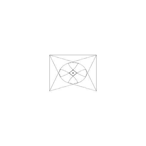
Figure 1: Square billiard in the 5-dimensional model with two internal spaces, scalar field and four “branes” (two electric and two magnetic).

This means that the points $\vec{v}^{s_{i}}$, $i=1,2,3,4$, form a square in $\mbox{\rm I$\!$R}^{2}$ containing $S^{1}$ ($\vec{v}^{s_{1}}=-\vec{v}^{s_{4}}$, $\vec{v}^{s_{2}}=-\vec{v}^{s_{3}}$), i.e. all points of $S^{1}$ are illuminated by these four points. The billiard $B$ (4.28) is a sub-compact square ($\bar{B}$ is compact) in the Lobachevsky space. For $d=2$ ($D=5$) it is depicted on Fig. 1.

5.2 Billiard is a triangle

Let us consider a model defined on

$$M=\mbox{\rm I$\!$R}\times M_{1}\times M_{2}\times M_{3}$$ (5.7)

and governed by the Lagrangian

$${\cal L}={R}[g]-2\Lambda-\frac{1}{n_{1}!}(F^{1})^{2}_{g},$$ (5.8)

where $d_{i}=\dim M_{i}=d$, $n_{1}=d+1$, $d\geq 2$, $w=-1$, $\varepsilon(i)=1$, $i=1,2,3$, and $D=1+3d$. Let

$$s_{1}=(1,e,\{1\}),\quad s_{2}=(1,e,\{2\}),\quad s_{3}=(1,e,\{3\}),$$ (5.9)

i.e. we have three electric branes corresponding to the form $F^{1}$. The brane $s_{i}$ “lives” in $M_{i}$, $i=1,2,3$.

From (4.48) we get

$$(\vec{v}^{s_{i}})^{2}=6d-2,$$ (5.10)

$$\vec{v}^{s_{i}}\vec{v}^{s_{j}}=1-3d,$$ (5.11)

$i\neq j$; $i,j=1,2,3$.

For $d\geq 2$ the points $\vec{v}^{s_{i}}$, $i=1,2,3$, form a triangle in $\mbox{\rm I$\!$R}^{2}$ containing $S^{1}$ and all points of $S^{1}$ are illuminated by these three points. The billiard (4.28) is a sub-compact triangle in the Lobachevsky space $D^{2}$. For $d=2$ it is depicted on Fig. 2.

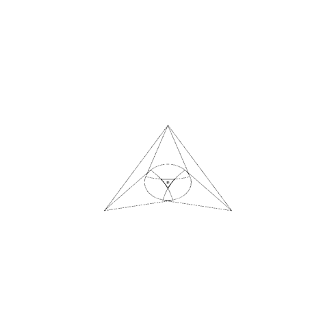
Figure 2: Triangle billiard in the 7-dimensional model with three internal spaces and three electric “branes”.

For $d=1$ we obtain (at least formally) the billiard $B$ depicted on Fig. 3. The closure of $B$ is not compact but the area of $B$ is finite. This billiard appears in the well-known Bianchi-IX model (for a review, see [39, 40, 45]). For $d=1$ the restriction on composite $p$-branes (3.1) is not satisfied but to avoid this obstacle we may consider non-composite case when the Lagrangian (5.8) is replaced by the following Lagrangian in the dimension $D=4$ with three 2-forms $F^{a}$, $a=1,2,3$,

$${\cal L}={R}[g]-2\Lambda-\sum_{a=1}^{3}\frac{1}{2!}(F^{a})^{2}_{g},$$ (5.12)

and the relation (5.9) is replaced by its non-composite analogue:

$$s_{1}=(1,e,\{1\}),\quad s_{2}=(2,e,\{2\}),\quad s_{3}=(3,e,\{3\}).$$ (5.13)

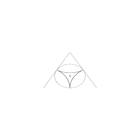
Figure 3: Triangle billiard for $D=4$ coinciding with that of Bianchi-IX model.

6 $D=11$ supergravity

6.1 “Truncated” $D=11$ supergravity

Now we consider a “truncated” bosonic sector of $D=11$ supergravity governed by the action (“truncated” means without Chern-Simons terms)

$$S_{tr}=\int d^{11}z\sqrt{|g|}\biggl{\{}R[g]-\frac{1}{4!}F^{2}_{g}\biggr{\}}$$ (6.1)

where $F=dA=F^{1}$ is a 4-form. In this case we have electric 2-branes ($d(I_{s})=3$) and magnetic 5-branes ($d(I_{s})=6$).

From (4.48) we get

$$(\vec{v}^{s})^{2}=21,\qquad v_{s}=e,$$ (6.2)

$$(\vec{v}^{s})^{2}=6,\qquad v_{s}=m,$$ (6.3)

and

$$\vec{v}^{s}\vec{v}^{s^{\prime}}= =1+10[d(I_{s}\cap I_{s^{\prime}})-1],\qquad v_{s}=v_{s^{\prime}}=e,$$ (6.5)

$$=1+\frac{5}{2}[d(I_{s}\cap I_{s^{\prime}})-4],\qquad v_{s}=v_{s^{\prime}}=m,$$

$$=1+5[d(I_{s}\cap I_{s^{\prime}})-2],\qquad v_{s}=e,\ v_{s^{\prime}}=m.$$ (6.6)

Scalar products (6.2)-(6.6) are (in some sense) “building blocks” for constructing billiards for the model under consideration.

Now we suggest an example of a billiard with a finite volume that occurs in the truncated $D=11$ supergravity. Let us consider the metric (2.8) defined on the manifold

$$M=\mbox{\rm I$\!$R}\times M_{1}\times\ldots\times M_{5},$$ (6.7)

where all $(M_{i},g^{i})$, $i=1,\ldots,5$, are 2-dimensional Einstein manifolds of the Euclidean signature and $w=-1$.

We consider ten magnetic $5$-branes wrapped on six-dimensional “submanifolds” $M_{i}\times M_{j}\times M_{k}$, $1\leq i<j<k\leq 5$. Thus, the $5$-branes are labeled by indices

$$s=s(i,j,k)=(1,m,\{i,j,k\}),$$ (6.8)

$1\leq i<j<k\leq 5$.

It follows from (6.3) and (6.5) that all vectors $\vec{v}^{s}$ have the same length: $|\vec{v}^{s}|=\sqrt{6}$ and $\vec{v}^{s}\vec{v}^{s^{\prime}}=1,-4$ for dimensions of intersections $d(I_{s}\cap I_{s^{\prime}})=4,2$ respectively.

Now we prove that in our case the set of sources located at points $\vec{v}^{s}\in\mbox{\rm I$\!$R}^{4}$, $s\in S=S_{m}$ “illuminates” the 3-dimensional (Kasner) sphere $S^{3}$ and hence (according to the Proposition from Section 4) the 4-dimensional billiard (4.28) $B\subset D^{4}$ has a finite volume. Due to Proposition 2 from Section 4 it is sufficient to prove the following proposition.

Proposition 3. There are no $\alpha=(\alpha^{1},\ldots,\alpha^{5})\in\mbox{\rm I$\!$R}^{5}$ satisfying the relations

$$\sum_{i=1}^{5}\alpha^{i}=\sum_{i=1}^{5}(\alpha^{i})^{2}=\frac{1}{2},$$ (6.9)

and

$$\alpha^{i}+\alpha^{j}+\alpha^{k}>0,$$ (6.10)

for all $1\leq i<j<k\leq 5$.

This proposition is a consequence of the following statement.

Proposition 4. Let $\alpha=(\alpha^{1},\ldots,\alpha^{5})\in\mbox{\rm I$\!$R}^{5}$ satisfy the relations (6.9) and $\alpha_{1}\leq\alpha_{2}\leq\alpha_{3}\leq\alpha_{4}\leq\alpha_{5}$. Then

$$\alpha^{1}+\alpha^{2}+\alpha^{3}\leq 0,$$ (6.11)

and $\alpha^{1}+\alpha^{2}+\alpha^{3}=0$ only if $\alpha=\alpha_{1}$, where

$$\alpha_{1}=\left(-\frac{1}{2},\frac{1}{4},\frac{1}{4},\frac{1}{4},\frac{1}{4}\right).$$ (6.12)

Proof. Let us consider the set $K$ of Kasner vector parameters $\alpha=(\alpha^{1},\ldots,\alpha^{5})\in\mbox{\rm I$\!$R}^{5}$ satisfying (6.9). Let

$$G=\{\alpha\in K|\alpha^{1}<\alpha^{2}<\alpha^{3}<\alpha^{4}<\alpha^{5}\}$$ (6.13)

and

$$\bar{G}=\{\alpha\in K|\alpha^{1}\leq\alpha^{2}\leq\alpha^{3}\leq\alpha^{4}\leq\alpha^{5}\}.$$ (6.14)

$G$ is an open submanifold of the 3-dimensional “Kasner” manifold $K$ and $\bar{G}$ is a closure of $G$. $\bar{G}$ is compact subset of $K$. Let us consider a smooth function $f:\mbox{\rm I$\!$R}^{5}\rightarrow\mbox{\rm I$\!$R}$ defined by the relation

$$f(\alpha)=\alpha^{1}+\alpha^{2}+\alpha^{3}.$$ (6.15)

Let $f_{|}=f_{|\bar{G}}$ be a restriction of $f$ on $\bar{G}$. $f_{|}$ is a continuous function reaching an (absolute) maximum on the compact (topological) space $\bar{G}$:

$$C={\rm max}f_{|}=f(\alpha_{max}),$$ (6.16)

$\alpha_{max}\in\bar{G}$. It is clear that $C\geq 0$, since $C\geq f(\alpha_{1})=0$, where $\alpha_{1}$ is defined in (6.12). To prove the proposition it is sufficient to prove that the point of maximum $\alpha_{max}$ is unique and

$$\alpha_{max}=\alpha_{1}.$$ (6.17)

Let us prove the relation (6.17). The point $\alpha_{max}$ does not belong to $G$. Indeed, if we suppose that $\alpha_{max}\in G$ we get the conditional extremum relation

$$d\Phi(\alpha)=0$$ (6.18)

at $\alpha=\alpha_{max}$, where

$$\Phi(\alpha)=\Phi_{0}(\alpha)\equiv f(\alpha)+\lambda_{1}\sum_{i=1}^{5}\alpha^{i}+\lambda_{2}\sum_{i=1}^{5}(\alpha^{i})^{2},$$ (6.19)

and $\lambda_{1}$ and $\lambda_{2}$ are Langrange multipliers. It follows from (6.18) and (6.19) that

$$\partial_{i}\Phi=1+\lambda_{1}+2\lambda_{2}\alpha^{i}=0,\quad i=1,2,3,$$ (6.20)

$$\partial_{j}\Phi=\lambda_{1}+2\lambda_{2}\alpha^{j}=0,\quad j=4,5,$$ (6.21)

at $\alpha=\alpha_{max}$. Relations (6.20) and (6.21) imply $\lambda_{2}\neq 0$ and $\alpha^{4}=\alpha^{5}$. The latter contradicts the inequality $\alpha^{4}<\alpha^{5}$ for points in $G$. Thus, $\alpha_{max}\in\bar{G}\setminus G$. The set $\partial G=\bar{G}\setminus G$ is a border of the curved tetrahedron $\bar{G}$. It is a union of four faces

$$\alpha^{1}=\alpha^{2}<\alpha^{3}<\alpha^{4}<\alpha^{5}\quad(\Gamma_{1}),$$ (6.22)

$$\alpha^{1}<\alpha^{2}=\alpha^{3}<\alpha^{4}<\alpha^{5}\quad(\Gamma_{2}),$$ (6.23)

$$\alpha^{1}<\alpha^{2}<\alpha^{3}=\alpha^{4}<\alpha^{5}\quad(\Gamma_{3}),$$ (6.24)

$$\alpha^{1}<\alpha^{2}<\alpha^{3}<\alpha^{4}=\alpha^{5}\quad(\Gamma_{4}),$$ (6.25)

six edges

$$\alpha^{1}=\alpha^{2}=\alpha^{3}<\alpha^{4}<\alpha^{5}\quad(E_{12}),$$ (6.26)

$$\alpha^{1}=\alpha^{2}<\alpha^{3}=\alpha^{4}<\alpha^{5}\quad(E_{13}),$$ (6.27)

$$\alpha^{1}=\alpha^{2}<\alpha^{3}<\alpha^{4}=\alpha^{5}\quad(E_{14}),$$ (6.28)

$$\alpha^{1}<\alpha^{2}=\alpha^{3}=\alpha^{4}<\alpha^{5}\quad(E_{23}),$$ (6.29)

$$\alpha^{1}<\alpha^{2}=\alpha^{3}<\alpha^{4}=\alpha^{5}\quad(E_{24}),$$ (6.30)

$$\alpha^{1}<\alpha^{2}<\alpha^{3}=\alpha^{4}=\alpha^{5}\quad(E_{34}),$$ (6.31)

and four vertices

$$\alpha^{1}<\alpha^{2}=\alpha^{3}=\alpha^{4}=\alpha^{5}\quad(V_{1}),$$ (6.32)

$$\alpha^{1}=\alpha^{2}<\alpha^{3}=\alpha^{4}=\alpha^{5}\quad(V_{2}),$$ (6.33)

$$\alpha^{1}=\alpha^{2}=\alpha^{3}<\alpha^{4}=\alpha^{5}\quad(V_{3}),$$ (6.34)

$$\alpha^{1}=\alpha^{2}=\alpha^{3}=\alpha^{4}<\alpha^{5}\quad(V_{4}).$$ (6.35)

The point of maximum $\alpha_{max}$ does not belong to any face $\Gamma_{a}$, $a=1,2,3,4$. Indeed, if we suppose that $\alpha_{max}$ belongs to some face $\Gamma_{a}$ we get the conditional extremum relation (6.18) with modified $\Phi$:

$$\Phi=\Phi_{0}+\lambda_{3}(\alpha^{a}-\alpha^{a+1}),$$ (6.36)

$a=1,2,3,4$. But one may verify that there are no solutions of the relation (6.18) in this case. Analogous arguments lead us to a non-existence of points of maximum among the points of edges $E_{12},E_{13},E_{14},E_{23},E_{24},E_{34}$. Here the only difference is that there exist (only) two extremal points belonging to $E_{13}$ and $E_{23}$ respectively:

$$\alpha^{1}=\alpha^{2}=\frac{1}{10}\left(1-\frac{12}{\sqrt{14}}\right),\alpha^{3}=\alpha^{4}=\frac{1}{10}\left(1+\frac{3}{\sqrt{14}}\right),\alpha^{5}=\frac{1}{10}\left(1+\frac{18}{\sqrt{14}}\right),$$ (6.37)

$$\alpha^{1}=\frac{1}{10}\left(1-\frac{3}{2}\sqrt{6}\right),\alpha^{2}=\alpha^{3}=\alpha^{4}=\frac{1}{10}\left(1-\frac{1}{4}\sqrt{6}\right),\alpha^{5}=\frac{1}{10}\left(1+\frac{9}{4}\sqrt{6}\right),$$ (6.38)

but $f(\alpha)<0$ in these points and hence they are not the points of maximum. Thus, $\alpha_{max}$ belongs to the set of vertices:

$$\alpha^{1}=-\frac{1}{2},\quad\alpha^{2}=\alpha^{3}=\alpha^{4}=\alpha^{5}=\frac{1}{4}\quad(V_{1}),$$ (6.39)

$$\alpha^{1}=\alpha^{2}=\frac{1}{10}\left(1-\frac{3}{2}\sqrt{6}\right),\quad\alpha^{3}=\alpha^{4}=\alpha^{5}=\frac{1}{10}\left(1+\sqrt{6}\right)\quad(V_{2}),$$ (6.40)

$$\alpha^{1}=\alpha^{2}=\alpha^{3}=\frac{1}{10}\left(1-\sqrt{6}\right),\quad\alpha^{4}=\alpha^{5}=\frac{1}{10}\left(1+\frac{3}{2}\sqrt{6}\right)\quad(V_{3}),$$ (6.41)

$$\alpha^{1}=\alpha^{2}=\alpha^{3}=\alpha^{4}=-\frac{1}{20},\quad\alpha^{5}=\frac{7}{10}\quad(V_{4}).$$ (6.42)

The calculation gives us $f(\alpha)<0$ for $\alpha=V_{i}$, $i=2,3,4$. Thus, the first vertex $V_{1}=\alpha_{1}$ is the point of maximum. The Proposition 4 is proved.

We also proved the Proposition 3 (as a consequence of the Proposition 4) and due to Proposition 2 the following proposition.

Proposition 5. For the model (6.1)-(6.8) the Kasner sphere $S^{3}$ is illuminated by the set of ten sources located at points $\vec{v}^{s}\in\mbox{\rm I$\!$R}^{4}$ from (4.30) , with $s=s(i,j,k)$, $1\leq i<j<k\leq 5$, defined in (6.8), and hence the billiard $B$ (4.28) has a finite volume.

Moreover, this proposition may be strengthen as follows.

Proposition 5a. In terms of Proposition 5 all points of the Kasner $S^{3}$ sphere except five points $\vec{n}_{1},\ldots,\vec{n}_{5}\in S^{3}$ corresponding to the Kasner sets

$$\alpha_{1}=\left(-\frac{1}{2},\frac{1}{4},\frac{1}{4},\frac{1}{4},\frac{1}{4}\right),\ldots,\alpha_{5}=\left(\frac{1}{4},\frac{1}{4},\frac{1}{4},\frac{1}{4},-\frac{1}{2}\right)\in K,$$ (6.43)

respectively (see (4.44)) are strongly illuminated by the set of ten sources $\vec{v}^{s}\in\mbox{\rm I$\!$R}^{4}$, $s\in S$.

Proof. The set $K$ of Kasner parameters satisfying (6.9) is a union of $5!=120$ “sectors”

$$K=K_{12345}\cup K_{21345}\cup\ldots\cup K_{54321},$$ (6.44)

where

$$K_{i_{1}i_{2}i_{3}i_{4}i_{5}}=\bar{G}=\{\alpha\in K|\alpha^{i_{1}}\leq\alpha^{i_{2}}\leq\alpha^{i_{3}}\leq\alpha^{i_{4}}\leq\alpha^{i_{5}}\}$$ (6.45)

and $(i_{1},i_{2},i_{3},i_{4},i_{5})$ is a permutation of $(1,2,3,4,5)$. Due to Proposition 1a and Proposition 4 any point $\vec{n}=\vec{n}(\alpha)\in S^{3}$ corresponding to $\alpha\in K_{12345}\setminus\{\alpha_{1}\}$ is strongly illuminated by the source located at point $\vec{v}^{s}$, with $s=s(1,2,3)$. Analogously, any point $\vec{n}=\vec{n}(\alpha)\in S^{3}$ corresponding to $\alpha\in K_{i_{1}i_{2}i_{3}i_{4}i_{5}}\setminus\{\alpha_{i_{1}}\}$ is strongly illuminated by the source located at point $\vec{v}^{s}$, with $s=s(i_{1},i_{2},i_{3})$, where $(i_{1},i_{2},i_{3},i_{4},i_{5})$ is a permutation of $(1,2,3,4,5)$. The proposition is proved.

The points $\vec{n}_{1},\ldots,\vec{n}_{5}$ from Proposition 5a are not strongly illuminated (see Proposition 1a). Thus, Proposition 5, Proposition 5a and Proposition (from Section 4) imply that the billiard $B$ (4.28) has a finite volume but its closure $\bar{B}$ is not compact. Points $\vec{n}_{1},\ldots,\vec{n}_{5}\in S^{3}$ are ending points of five “horns” of $B$. (These “horns” look similar to potential energy “valleys” that occur in some toy models, e.g. related to M(atrix) theory [51]).

Using relations (4.44) one may verify that

$$\vec{n}_{i}\vec{n}_{j}=-\frac{1}{4},\quad i\neq j,$$ (6.46)

$i,j=1,\ldots,5$. This means that $\vec{n}_{1},\ldots,\vec{n}_{5}$ are vertices of a 4-dimensional simplex.

Here we considered the billiard $B$ generated by ten sources, corresponding to non-zero charges : $Q_{s}\neq 0$, $s\in S$. If some charges are zero: $Q_{s}=0$, $s\in S_{0}$, then the corresponding points $\vec{v}^{s}$, $s\in S_{0}$ ($S_{0}\neq\emptyset$) are “switched off” and billiard is generated by $m\leq 9$ point-like sources. In this case we have the following proposition.

Proposition 5b. In terms of Proposition 5 any subset of sources $\vec{v}^{s}$, $s\in S\setminus S_{0}$, with $S_{0}\neq\emptyset$, does not illuminate the Kasner sphere $S^{3}$ and hence the billiard $B$ generated by this subset has an infinite volume.

Proof. Without a loss of generality let us suppose that $S_{0}$ contains $s(1,2,3)$, i.e. at least the source at $\vec{v}^{s}$, $s=s(1,2,3)$, is “switched off”. Then, the point $\vec{n}$ corresponding to the set $\alpha=(\alpha^{i})$ from (6.41) belongs to the shadow, since

$$\alpha^{i}+\alpha^{j}+\alpha^{k}>0,$$ (6.47)

for all $1\leq i<j<k\leq 5$, $(i,j,k)\neq(1,2,3)$. Thus, the shadow set is non-empty. (This set is open since it is an intersection of a finite number of open shadow sets corresponding to sources of light.) The proposition is proved.

6.2 Inclusion of Chern-Simons term

Now we consider the total bosonic sector action for $D=11$ supergravity with the Chern-Simons term included:

$$S=S_{tr}+c\int_{M}A\wedge F\wedge F$$ (6.48)

where $S_{tr}$ is defined in (6.1), $c={\rm const}$, ($F=dA$). Since the second term in (6.48) (Chern-Simons term) does not depend upon a metric the Einstein equations are not changed. The only modification of equations of motion is related to “Maxwell” equations

$$d*F={\rm const}\ F\wedge F.$$ (6.49)

Due to (6.49) solutions to field equations corresponding to the truncated model (6.1) with the trivial Chern-Simons term

$$F\wedge F=0.$$ (6.50)

are also solutions for $D=11$ supergravity.

Now, we are interested in existence of solutions for the truncated model with non-zero charges $Q_{s}\neq 0$ satisfying (6.50).

Calculating the Hodge dual in (2.20) and using the solution (3.34) we get

$$F=-e^{f}\sum_{s\in S}Q_{s}\tau(\bar{I}_{s}),\quad f=2\sum_{i=1}^{5}x^{i}-\gamma,$$ (6.51)

where $\bar{I}_{s}=\{1,2,3,4,5\}\setminus I_{s}$, $s\in S=S_{m}$, and $S$ is the index set defined in (6.8). For the Chern-Simons term we obtain

$$e^{-2f}F\wedge F=2\sum_{i=1}^{5}P_{i}\tau(\bar{\{i\}}),$$ (6.52)

where

$$2P_{i}=\sum_{s,s^{\prime}\in S}Q_{s}Q_{s^{\prime}}\delta(I_{s}\cap I_{s^{\prime}},\{i\}),$$ (6.53)

$i=1,2,3,4,5$. Here $\delta(A,B)=1$ for $A=B$, $\delta(A,B)=0$ otherwise.

Proposition 6. Let all charges be non-zero: $Q_{s}\neq 0$ for all $s\in S$. Then

$$(F\wedge F)(z)\neq 0,$$ (6.54)

in all points $z\in M$.

Proof. Let us suppose that the Chern-Simons term vanishes in some point (i.e. relation (6.50) in some point is satisfied). Since forms $\tau(\bar{\{i\}})$ are linearly independent at any point, we obtain $P_{i}=0$, $i=1,2,3,4,5$, or explicitly

$$P_{1}=Q_{123}Q_{145}+Q_{124}Q_{135}+Q_{125}Q_{134}=0,$$ (6.55)

$$P_{2}=Q_{123}Q_{245}+Q_{124}Q_{235}+Q_{125}Q_{234}=0,$$ (6.56)

$$P_{3}=Q_{123}Q_{345}+Q_{134}Q_{235}+Q_{135}Q_{234}=0,$$ (6.57)

$$P_{4}=Q_{124}Q_{345}+Q_{134}Q_{245}+Q_{145}Q_{234}=0,$$ (6.58)

$$P_{5}=Q_{125}Q_{345}+Q_{135}Q_{245}+Q_{145}Q_{235}=0,$$ (6.59)

where we denote $Q_{ijk}=Q_{s}$ for $s=s(i,j,k)$, $1\leq i<j<k\leq 5$. Let us denote $k_{2}=Q_{345}$, $k_{3}=Q_{245}$, $k_{4}=Q_{235}$, $k_{5}=Q_{234}$ and $a=Q_{145}$, $b=Q_{135}$. From (6.59) we get

$$Q_{125}=-\frac{k_{3}}{k_{2}}b-\frac{k_{4}}{k_{2}}a.$$ (6.60)

From the relation $k_{3}P_{3}+k_{4}P_{4}+k_{5}P_{5}=0$ we get

$$Q_{134}=-\frac{k_{5}}{k_{4}}b-\frac{k_{5}}{k_{3}}a.$$ (6.61)

From (6.57)and (6.58) we deduce

$$Q_{123}=\frac{k_{4}k_{5}}{k_{2}k_{3}}a,\quad Q_{124}=\frac{k_{3}k_{5}}{k_{2}k_{4}}b.$$ (6.62)

Substituting (6.60)-(6.62) into eq. (6.55) we get

$$(k_{4}a)^{2}+(k_{3}b)^{2}+(k_{4}a+k_{3}b)^{2}=0.$$ (6.63)

Hence $a=b=0$. But this contradicts our supposition, that $Q_{s}\neq 0$. So, the proposition is proved.

Thus, it follows from Proposition 5b and Proposition 6, that the inclusion of the Chern-Simons term leads us to the billiard $B$ of infinite volume. In this case some Kasner (shadow) zones are opened and we have the Kasner-like behaviour near the singularity.

7 Discussions

In this paper we considered the behaviour near the singularity of the multidimensional model describing the cosmological evolution of several Einstein spaces in the theory with scalar fields and fields of forms. Using the results from [43, 44, 45] we obtained the billiard representation on multidimensional Lobachevsky space for the cosmological model near the singularity. We suggested and studied examples with oscillating behaviour near the singularity in the model with four $p$-branes and a square billiard and in the model with three $p$-branes, when the billiard is a triangle (like it takes place in Bianchi-IX model). A 4-dimensional billiard with a finite volume in the “truncated” $D=11$ supergravity was also considered. It was shown that the inclusion of the Chern-Simons term leads to the destruction of some confining walls of the billiard.

Acknowledgments.

This work was supported in part by the Russian Ministry for Science and Technology and Russian Fund for Basic Research, project N 98-02-16414. V.N.M. is grateful to the Dept. Math., University of Aegean for the kind hospitality during his stay in Karlovassi, Greece in December 1998 - January 1999.

References

-
[1]
C. Hull and P. Townsend, Unity of Superstring Dualities,
Nucl. Phys. B 438, 109 (1995).
P. Horava and E. Witten, Nucl. Phys. B 460, 506 (1996). - [2] J.M. Schwarz, Lectures on Superstring and M-Theory Dualities, hep-th/9607201;
- [3] M.J. Duff, M-theory (the Theory Formerly Known as Strings), hep-th/9608117.
- [4] C. Vafa, Evidence for F-Theory, hep-th/9602022; Nucl. Phys. B 469, 403 (1996).
- [5] M.B. Green, J.H. Schwarz and E. Witten, Superstring Theory (Cambridge University Press., Cambridge, 1987).
- [6] V.D. Ivashchuk and V.N. Melnikov, Sigma-Model for Generalized Composite p-branes, hep-th/9705036; Class. and Quantum Grav. 14, 11, 3001 (1997).
- [7] M.J. Duff, R.R. Khuri and J.X. Lu, Phys. Rep. 259, 213 (1995).
- [8] K.S. Stelle, Lectures on Supergravity p-Branes, hep-th/9701088; hep-th/9608117.
- [9] E. Bergshoeff, M. de Roo, E. Eyras, B. Janssen and J.P. van der Schaar, Class. Quantum Grav. 14, 2757 (1997). hep-th/9604120.
- [10] I.Ya. Aref’eva and A.I. Volovich, Class. Quantum Grav. 14 (11), 2990 (1997); hep-th/9611026.
- [11] I.Ya. Aref’eva and O.A. Rytchkov, Incidence Matrix Description of Intersecting p-brane Solutions, hep-th/9612236.
- [12] V.D. Ivashchuk and V.N. Melnikov, Intersecting p-Brane Solutions in Multidimensional Gravity and M-Theory, hep-th/9612089; Grav. and Cosmol. 2, No 4, 297 (1996).
- [13] V.D. Ivashchuk and V.N. Melnikov, Phys. Lett. B 403, 23 (1997).
- [14] V.D. Ivashchuk, V.N. Melnikov and M. Rainer, Multidimensional Sigma-Models with Composite Electric p-branes, gr-qc/9705005; Gravit. and Cosm. 4, No 1 (13) (1998).
- [15] V.D. Ivashchuk and V.N. Melnikov, Mudjumdar-Papapetrou Type Solutions in Sigma-model and Intersecting -branes, hep-th/9702121, Class. and Quantum Grav. 16, 849-869 (1999).
- [16] V.D. Ivashchuk and V.N. Melnikov, Multidimensional Classical and Quantum Cosmology with Intersecting -branes, hep-th/9708157; J. Math. Phys., 39, 2866 (1998).
- [17] H. Lü, S. Mukherji, C.N. Pope and K.-W. Xu, Cosmological Solutions in String Theories, hep-th/9610107.
- [18] V.D. Ivashchuk and V.N. Melnikov, Multidimensional cosmology with -component perfect fluid, gr-qc/ 9403063; Int. J. Mod. Phys. D 3, 795 (1994).
- [19] V.R. Gavrilov, V.D. Ivashchuk and V.N. Melnikov, Integrable pseudo-euclidean Toda-like systems in multidimensional cosmology with multicomponent perfect fluid, J. Math. Phys 36, 5829 (1995).
- [20] H. Lü, C.N. Pope, and K.W. Xu, Liouville and Toda Solitons in M-Theory, hep-th/9604058.
- [21] K.A. Bronnikov, M.A. Grebeniuk, V.D. Ivashchuk and V.N. Melnikov, Integrable Multidimensional Cosmology for Intersecting -branes, Grav. and Cosmol. 3, No 2(10), 105 (1997).
- [22] M.A. Grebeniuk, V.D. Ivashchuk and V.N. Melnikov, Integrable Multidimensional Quantum Cosmology for Intersecting p-Branes, Grav. and Cosmol. 3, No 3 (11), 243 (1997), gr-qc/9708031.
- [23] K.A. Bronnikov, V.D. Ivashchuk and V.N. Melnikov, The Reissner-Nordström Problem for Intersecting Electric and Magnetic p-Branes, gr-qc/9710054; Grav. and Cosmol. 3, No 3 (11), 203 (1997).
- [24] K.A. Bronnikov, Block-orthogonal Brane systems, Black Holes and Wormholes, hep-th/9710207; Grav. and Cosmol. 4, No 2 (14), (1998).
- [25] V.D. Ivashchuk and V.N. Melnikov, Multidimensional Cosmological and Spherically Symmetric Solutions with Intersecting -branes, gr-qc/9901001.
- [26] V.D. Ivashchuk, V.N. Melnikov and A.I. Zhuk, Nuovo Cimento B 104, 575 (1989).
- [27] C.W. Misner, Phys. Rev. 186, 1319 (1969).
- [28] V.A. Belinskii, E.M. Lifshitz and I.M. Khalatnikov, Usp. Fiz. Nauk 102, 463 (1970) [in Russian]; Adv. Phys. 31, 639 (1982).
- [29] D.M. Chitre, Ph. D. Thesis (University of Maryland) 1972.
- [30] C. Misner, K. Thorne and J. Wheeler, Gravitation (San Francisco, Freeman & Co.) 1972.
- [31] V.A. Belinskii and I.M. Khalatnikov, ZhETF, 63, 1121 (1972).
- [32] J.D. Barrow and J. Stein-Schabes, Phys. Rev. D 32, 1595 (1985).
- [33] J. Demaret, M. Henneaux and P. Spindel, Phys. Lett. B 164 27 (1985).
- [34] M. Szydlowski and G. Pajdosz, Class. Quant. Grav. 6, 1391 (1989).
- [35] J. Demaret, J.-L. Hanquin, M. Henneaux, P. Spindel and A. Taormina, Phys. Lett. B 175, 129 (1986).
- [36] J. Demaret, Y. De Rop and M. Henneaux, Phys. Lett. 211B, 37 (1988).
- [37] M. Szydlowski, J. Szczesny and M. Biesiada, GRG 19, 1118 (1987).
- [38] S. Cotsakis, J. Demaret, Y. De Rop and L. Querella, Phys. Rev. D 48, 4595 (1993).
- [39] J. Pullin, Time and Chaos in General Relativity preprint Syracuz. Univ. Su-GP-91/1-4., 1991; 1991 in Relativity and Gravitation: Classical and Quantum, Proc. of SILARG VII Cocoyos Mexico 1990 (Singapore, World Scientific) ed. D’Olivo J C et al.
- [40] A.A. Kirillov, ZhETF 76, 705 (1993) (in Russian).
- [41] A.A. Kirillov, ZhETF 55, 561 (1992); Int. Journ. Mod. Phys. D 3, 1 (1994).
- [42] C.W. Misner, The Mixmaster cosmological metrics, preprint UMCP PP94-162, 1994; gr-qc/9405068.
- [43] V.D. Ivashchuk, A.A. Kirillov and V.N. Melnikov, Izv. Vuzov (Fizika) No 11, 107 (1994) (in Russian).
- [44] V.D. Ivashchuk, A.A. Kirillov and V.N. Melnikov, Pis’ma ZhETF 60, No 4, 225 (1994) (in Russian).
- [45] V.D. Ivashchuk and V.N. Melnikov, Billiard representation for multidimensional cosmology with multicomponent perfect fluid near the singularity, Class. Quantum Grav. 12, 809 (1995).
- [46] A.A. Kirillov and V.N. Melnikov, On Properties of Metrics Inhomogeneouties in the Vicinity of a Singularity in K-K Cosmological Models, Astron. Astrophys. Trans., 10, 101 (1996).
- [47] P.S. Soltan, Izv. AN Moldav. SSR , 1, 49 (1963) (in Russian).
- [48] V.G. Boltyansky and I.Z. Gohberg, Theorems and Problems of Kombinatorial Geometry (Moscow, Nauka) 1965 (in Russian).
- [49] L. Fejes Toth, Lagerungen in der Ebene auf der Kugel und Raum (Berlin, Springer) 1953.
- [50] C.A. Rogers, Mathematika 10, 157 (1963).
- [51] I.Ya. Aref’eva, P.B. Medvedev, O.A. Rytchkov and I.V. Volovich, Chaos in M(atrix) Theory, hep-th/9710032.