Abstract

It is shown that a large class of higher-order (i.e. non-quadratic) scalar kinetic terms can, without the help of potential terms, drive an inflationary evolution starting from rather generic initial conditions. In many models, this kinetically driven inflation (or “$k$-inflation” for short) rolls slowly from a high-curvature initial phase, down to a low-curvature phase and can exit inflation to end up being radiation-dominated, in a naturally graceful manner. We hope that this novel inflation mechanism might be useful in suggesting new ways of reconciling the string dilaton with inflation.

I Introduction

The inflationary paradigm [1] offers the attractive possibility of resolving many of the puzzles of standard hot big bang cosmology. The crucial ingredient of most successful inflationary scenarios is a period of “slow-roll” evolution of a scalar field $\varphi$ (the “inflaton”), during which the potential energy $V(\varphi)$ stored in $\varphi$ dominates its kinetic energy $\dot{\varphi}^{2}/2$ and drives a quasi-exponential expansion of the Universe. At present there exists no preferred concrete inflationary scenario based on a convincing realistic particle physics model. In particular, though string theory provides one with several very weakly coupled scalar fields (the moduli), which could be natural inflaton candidates, their non-perturbative potentials $V(\varphi)$ do not seem fit to sustain slow-roll inflation because, for large values of $\varphi$, they tend either to grow, or to tend to zero, too fast. It is therefore important to explore novel possibilities for implementing an inflationary evolution of the early Universe.

The aim of this work is to point out that, even in absence of any potential energy term, a general class of non-standard (i.e. non-quadratic) kinetic-energy terms $\mathcal{L}(\dot{\varphi})$, for a scalar field $\varphi$, can drive an inflationary evolution of the same type as the usually considered potential driven inflation. By “usual type of inflation” we mean here an accelerated expansion (in the Einstein conformal frame) during which the curvature scale starts around a Planckian value and then decreases monotonously. By contrast, the pre-big bang scenario [2] uses a standard (quadratic) kinetic-energy term $\dot{\varphi}^{2}/2$ to drive an accelerated contraction (in the Einstein frame) during which the curvature scale increases. Though we shall motivate below the consideration of non-standard kinetic terms by appealing to the existence, in string theory, of higher-order corrections to the effective action for $\varphi$, we do not claim that the structure needed for implementing our “kinetically driven” inflation arises inevitably in string theory. The aim of this work is more modest. We draw attention to a new mechanism for implementing inflation. A large class of the (toy) models we shall consider satisfy two of the most crucial requirements of inflationary scenarios: (i) the scalar perturbations are “well-behaved” during the inflationary stage, and (ii) there exist natural mechanisms for exiting inflation in a “graceful” manner. We leave to future work a more detailed analysis of the observational consequences of our kinetically driven inflation (spectrum of scalar and tensor perturbations, reheating, …). We hope that, by enlarging the basic “tool-kit” of inflationary cosmology, our mechanism could help to locate which sector of string-theory (if any) has inflated a strongly curved initial state into our presently observed large and weakly curved Universe.

II General Model

We consider a single scalar field $\varphi$ interacting with gravity through non-standard kinetic terms,

$$S=\int d^{4}x\,\sqrt{g}\left[-\frac{R}{6\kappa^{2}}+p(\varphi,\nabla\varphi)\right].$$ (2.1)

Here, $\kappa^{2}\equiv 8\pi G/3$ and we use the signature $(+---)$. For simplicity, we only consider Lagrangians $p$ which are local functions of $\nabla_{\mu}\varphi$ and therefore, depend only on the scalar

$$X\equiv\frac{1}{2}(\nabla\varphi)^{2}.$$ (2.2)

As we bar here the consideration of potential terms, we must impose that the function $p(\varphi,X)$ vanish when $X\rightarrow 0$. Near $X=0$, a generic kinetic Lagrangian $p(\varphi,X)$ is expected to admit an expansion of the form

$$p(\varphi,X)=K(\varphi)X+L(\varphi)X^{2}+\cdots.$$ (2.3)

One of the possible particle theory motivations for taking this kind of Lagrangian seriously could be the following. Let us consider only gravity and some moduli field $\varphi$ (which could be the dilaton, or some other moduli) in string theory. It is well-known that $\alpha^{\prime}$ corrections (due to the massive modes of the string) generate a series of higher-derivative terms in the low-energy effective action $S_{\rm eff}$, while string-loop corrections generate a non-trivial moduli dependence of the coefficients of the various kinetic terms. This leads to a structure of the type (in the string frame $\hat{g}_{\mu\nu}$)

$$S_{\rm eff} = \frac{1}{6\kappa^{2}}\int d^{4}x\sqrt{\hat{g}}\Big{\{}-B_{g}(\varphi)\hat{R}-B_{\varphi}^{(0)}(\hat{\nabla}\varphi)^{2}$$

$$+\alpha^{\prime}\left[c_{1}^{(1)}B_{\varphi}^{(1)}(\varphi)(\hat{\nabla}\varphi)^{4}+\cdots\right]+O(\alpha^{\prime}\,{}^{2})\Big{\}},$$

where the ellipsis stands for other four-derivative terms (like $(\Box\varphi)^{2},\hat{R}_{\mu\nu\rho\sigma}^{2},\ldots)$. In the case where $\varphi$ is the dilaton the coupling functions are of the form

$$B_{g}(\varphi) = e^{-\varphi}+c_{g,0}+c_{g,1}e^{\varphi}+\cdots,$$

$$B_{\varphi}^{(0)}(\varphi) = e^{-\varphi}+c_{\varphi,0}+c_{\varphi,1}e^{\varphi}+\cdots,$$

$$B_{\varphi}^{(1)}(\varphi) = e^{-\varphi}+\cdots,$$

where the ellipsis contain higher contributions in $g_{\rm string}^{2}=e^{\varphi}$, including non-perturbative ones. Transforming Eq. (II) to the Einstein frame $g_{\mu\nu}=B_{g}(\varphi)\hat{g}_{\mu\nu}$, and neglecting the other possible four derivative terms in Eq. (II), leads to the effective action (2.1) with $\varphi$-kinetic terms of the form (2.3) where

$$K(\varphi) = 3\frac{B_{g}^{\prime}{}^{2}(\varphi)}{B_{g}^{2}(\varphi)}-2\frac{B_{\varphi}^{(0)}(\varphi)}{B_{g}(\varphi)},$$ (2.5)

$$L(\varphi) = c_{1}^{(1)}\frac{2\alpha^{\prime}}{3\kappa^{2}}B_{\varphi}^{(1)}(\varphi).$$ (2.6)

In the case where $\varphi$ is the dilaton (so that $g_{s}=e^{\varphi/2}$ is the string coupling), we have, in the weak-coupling limit $g_{s}^{2}=e^{\varphi}\ll 1$, $B_{g}(\varphi)\simeq B_{\varphi}^{(0)}(\varphi)\simeq B_{\varphi}^{(1)}(\varphi)\simeq e^{-\varphi}$ so that $K(\varphi)\simeq 1$ and $L(\varphi)\propto e^{-\varphi}$. However, when $g_{s}$ becomes of the order of unity it is not a priori excluded that $\ K(\varphi)$ and $L(\varphi)$ could become more complicated functions of $\varphi$. We shall give below some examples of such possible complicated behaviours.

Returning now to a general Lagrangian $p(\varphi,X)$ the “matter” energy-momentum tensor reads

$$T_{\mu\nu}\equiv\frac{2}{\sqrt{g}}\frac{\delta S_{\varphi}}{\delta g^{\mu\nu}}=\frac{\partial p(\varphi,X)}{\partial X}\nabla_{\mu}\varphi\nabla_{\nu}\varphi-p(\varphi,X)g_{\mu\nu}.$$ (2.7)

Equation (2.7) shows that, if $\nabla_{\mu}\varphi$ is time-like (i.e. $X>0$), our scalar field action is “equivalent” to a perfect fluid ($T_{\mu\nu}=(\varepsilon+p)u_{\mu}u_{\nu}-p\,g_{\mu\nu}$) with pressure

$$p=p(\varphi,X),$$ (2.8)

energy density

$$\varepsilon=\varepsilon(\varphi,X)\equiv 2X\frac{\partial p(\varphi,X)}{\partial X}-p(\varphi,X),$$ (2.9)

and four-velocity

$$u_{\mu}=\sigma\frac{\nabla_{\mu}\varphi}{\sqrt{2X}},$$ (2.10)

where $\sigma$ denotes the sign of $\dot{\varphi}=\nabla_{0}\varphi$.

As usual, in inflationary cosmology, we consider a flat background Friedmann model $ds^{2}=dt^{2}-a^{2}(t)d\mathbf{x}^{2}$ and an homogeneous background scalar field $X=\frac{1}{2}\dot{\varphi}^{2}$. A convenient minimal set of independent evolution equations for $a(t)$ and $\varphi(t)$ is (with $H\equiv\dot{a}/a$)

$$H^{2} = \kappa^{2}\varepsilon\,,$$ (2.11)

$$\dot{\varepsilon} = -3H(\varepsilon+p).$$ (2.12)

It will be also useful to refer to other (redundant) forms of the evolution equations:

$$\frac{\ddot{a}}{a} = -\frac{1}{2}\kappa^{2}(\varepsilon+3p)\,,$$ (2.13)

$$\frac{1}{a^{3}}\frac{d}{dt}(a^{3}\pi) = \dot{\pi}+3H\pi=\frac{\partial p}{\partial\varphi},$$ (2.14)

where $\pi\equiv\partial p/\partial\dot{\varphi}=\dot{\varphi}\,\partial p/\partial X$ denotes the momentum conjugate to $\varphi$. [Note that equation (2.9) reads $\varepsilon=\dot{\varphi}\partial p/\partial\dot{\varphi}-p$, which is the usual energy associated to the Lagrangian $p(\varphi,\dot{\varphi})$.]

In this work we shall only consider solutions of Eqs. (2.11)-(2.14) which describe an expanding Universe (in Einstein frame), that is $H>0.$ This reduces the evolution equations (2.11), (2.12) to the master equation

$$\dot{\varepsilon}=-3\sqrt{\varepsilon}(\varepsilon+p).$$ (2.15)

Here, and in the following, we use units such that $\kappa^{2}\equiv 8\pi G/3=1$. Note that, from Eq. (2.11), $\varepsilon$ was constrained to be positive.

III Kinetically Driven Inflation - Basic Idea

As a warm up, let us first consider the case where the Lagrangian $p$ depends only on $X=\frac{1}{2}(\nabla\varphi)^{2}$, and not on $\varphi$: $p=p(X)$. From Eq. (2.9), the energy-density depends also only on $X$: $\varepsilon(X)=2X\partial p/\partial X-p(X)$. In hydrodynamical language it means that we have here an “isentropic” fluid, with a general equation of state relating $p$ to $\varepsilon$: $p=f(\varepsilon)$. The master evolution equation can then be qualitatively solved by looking at the graph of the equation of state $p=f(\varepsilon)$. The shape of this graph depends very much on the shape of the function $p=p(X)$, or better, on the shape of the function $p=p(\psi)$ where $\psi\equiv\dot{\varphi}$, so that $X=\frac{1}{2}\psi^{2}$. Indeed, the relation

$$\varepsilon=\psi\partial p/\partial\psi-p$$ (3.1)

shows that $\varepsilon$ can be read geometrically off the graph $p=p(\psi)$. More precisely $-\varepsilon$ is the “intercept”of the tangent to the curve $p=p(\psi)$ at the point $\psi$, i.e. its intersection with the vertical axis $\psi=0$. The minus sign means that $\varepsilon$ is positive (negative) if the tangent intersects the vertical axis below (above) the $p=0$ horizontal axis. Therefore, if the function $p(\psi)=\frac{1}{2}K\psi^{2}+\frac{1}{4}L\psi^{4}+\cdots$ is, for instance, always convex, $\partial^{2}p/\partial\psi^{2}>0$, as will be the case if all the coefficients $K,L,\ldots$ appearing in the expansion (2.3) are positive, $p$ and $\varepsilon$ will be always positive. In such a case, Eq. (2.15) shows that $\varepsilon$ will monotonically decrease towards zero, and the evolution will be driven to the “attracting solution”

$$\varepsilon=H^{2}\approx\frac{1}{9t^{2}}\quad,\quad a\approx a_{0}\,t^{1/3}.$$ (3.2)

This attractor corresponds to the asymptotic equation of state $p\approx\varepsilon$ valid near $\varepsilon=0$ where the usual kinetic term $p\simeq\frac{1}{2}K\psi^{2}$ dominates. On the other hand, if the function $p(\psi)$ is non-convex and has some oscillatory behaviour as $\psi$ increases (i.e., if we consider the general case where the expansion coefficients $K,L,\ldots$ in Eq. (2.3) may take negative values) the graph $p=f(\varepsilon)$ can be more complicated and can allow for exponential-type inflationary behaviour. Let us first note that, because of Eq. (3.1), the extrema of the function $p=p(\psi)$ (or $p=p(X)$) correspond to values where $p=-\varepsilon$, i.e. to fixed points of the master evolution equation (2.15). For a general function $p=p(X)$ the graph of the (multiform) equation of state might resemble Fig.1.

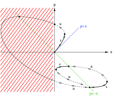
Figure 1: Graph of the equation of state linking $p$ to $\varepsilon$ for an hypothetical general kinetic Lagrangian $p(\dot{\varphi})$. The evolution for expanding, flat cosmologies proceeds along the indicated arrows. The shaded region ($\varepsilon<0$) is excluded. Except for the origin and the point above it on the vertical axis, the attractors of the evolution are inflationary fixed points with $p=-\varepsilon$.

From the master Eq. (2.15)  it follows that $\varepsilon$ will decrease above the line $p=-\varepsilon$, and increase below it. Fig. 1 then shows that all the intersection points with the $p=-\varepsilon$ line are attractors of the (future) evolution. The arrows in Fig. 1 indicate the evolutive flow, which reverses (along the graph) at the extrema of $\varepsilon$. The region where $\varepsilon<0$ is excluded because it cannot be reached by flat cosmologies (see Eq. (2.11)). The fixed points lying at the $p=-\varepsilon$ line correspond to an exponential inflation

$$H_{\rm att}^{2}=\varepsilon_{\rm fixed}\quad,\quad a_{\rm att}(t)=a_{0}\exp\left(\sqrt{\varepsilon_{\rm fixed}}t\right)$$ (3.3)

Apart from these inflationary attractors, there are two other attractors (in the case depicted in Fig. 1): (i) the origin, where the evolution is driven toward the solution (3.2) (corresponding to the “hard” equation of state $p=\varepsilon$), and (ii) the point above the origin on the vertical axis. As we will see later the latter point lies in the region of absolute instability and has therefore no physical significance.

In this work we shall focus on the inflationary attractors (3.3) because they exhibit the novel possibility of getting, for a large set of initial conditions, quasi-exponential (or power law) inflation out of a purely kinetic Lagrangian. Note that the condition for the existence of these inflationary attractors can also be seen in Eq. (2.14). In absence of a $\varphi$ dependence, Eq. (2.14) says that $a^{3}\pi$ is constant so that $\pi$ is attracted toward zero. As the momentum $\pi=\partial p/\partial\dot{\varphi}=\dot{\varphi}\,\partial p/\partial X$, we see that non trivial ($\dot{\varphi}\neq 0$) attractors can exist if the kinetic terms are non-standard so that $\partial p/\partial X$ can vanish for non zero values of $\dot{\varphi}$ . The extremal values of $p$ correspond to the inflationary attractors discussed above.

The labels “s” and “u” in Fig. 1 (which stand for “stable” and “unstable”) indicate whether, for our present isentropic equation of state $p=f(\varepsilon)$, the squared speed of sound $c_{s}^{2}=dp/d\varepsilon$ is positive or negative, respectively. This issue will be further discussed below.

Note that the “price” to pay for having inflationary attractors as in Fig. 1 is the existence of regions, in phase space $(\varphi,\dot{\varphi})$, with negative energy density. We shall assume in this work that this is not physically forbidden. All the cosmological evolutions that we shall consider below stay always in the positive energy regions, and the existence, elsewhere in phase space, of negative $\varepsilon$ regions does not necessarily cause some instabilities along our evolutionary tracks.

The simple case of a kinetic Lagrangian depending only on $\dot{\varphi}$ considered above is the analog, for kinetically driven inflation (or “k-inflation” for short), of a de Sitter model with constant energy density. It is clear that both models should have similar problems. Namely, there is no natural graceful exit, no smooth transition to a Friedmann Universe and the cosmological perturbations are “ill-defined”. To avoid these problems we should allow the coefficients in the expansion (2.3) of the Lagrangian $p$ to depend on the scalar field $\varphi$.

IV “Slow-Roll” k-Inflation

The simplest way to realize successfully the idea of k-inflation is to consider the analog of “slow-roll” potential driven inflation, in which the potential $V(\varphi)$ in the Lagrangian $\mathcal{L}(\varphi,\dot{\varphi})=\frac{1}{2}\dot{\varphi}^{2}-V(\varphi)$ dominates the kinetic term $\dot{\varphi}^{2}/2$ and evolves slowly. For the concept of k-inflation to have a relevance to a large class of models, we need to consider a general kinetic Lagrangian $p(\varphi,X)$. The idea is therefore to find the conditions under which the influence of the non-trivial $\varphi$ dependence of $p(\varphi,X)$ will represent only a relatively small perturbation of the attraction toward exponential inflation discussed in Section III. To do that in a concrete manner it is convenient to focus henceforth on the simplest kinetic Lagrangian, containing only $\dot{\varphi}^{2}$ and $\dot{\varphi}^{4}$ terms, namely

$$p(\varphi,X)=K(\varphi)X+L(\varphi)X^{2}=\frac{1}{2}K(\varphi)(\nabla\varphi)^{2}+\frac{1}{4}L(\varphi)(\nabla\varphi)^{4}.$$ (4.1)

Let us first motivate the possibility of rather arbitrary functions $K(\varphi),L(\varphi)$ by considering again the low-energy effective action of string theory (II). As we mentioned above, in the weak coupling limit $K(\varphi)\simeq 1$ and $L(\varphi)\propto e^{-\varphi}.$ However, when $g_{s}$ becomes of order unity it is not a priori excluded that $K(\varphi)$ could change sign. For instance we could consider a simple model (of the type considered in Refs. [3], [4]), where the coupling functions $B(\varphi)$ in the action (II) are the same, that is $B_{g}(\varphi)=B_{\varphi}^{(0)}(\varphi)=B_{\varphi}^{(1)}(\varphi)=B(\varphi)$. In this model

$$K(\varphi)=3\left(\frac{B^{\prime}(\varphi)}{B(\varphi)}\right)^{2}-2$$ (4.2)

might become negative when $g_{s}$ reaches values of order unity. In fact a model, incorporating string loop corrections, considered in Ref. [5] has

$$K(\varphi)=1-3k\,e^{\varphi}\frac{6+k\,e^{\varphi}}{(3+k\,e^{\varphi})^{2}},$$ (4.3)

where $k=3\delta^{\rm GS}/8\pi^{2}$ is a positive parameter. The R.H.S. of Eq. (4.3) becomes negative when $e^{\varphi}>3(\sqrt{6}-2)/2k$. Motivated by these examples, we shall assume, as simplest toy model exhibiting interesting dynamics, a Lagrangian of the form (4.1) with a function $K(\varphi)$ which is positive in some range of values of $\varphi$ (“weak-coupling-domain”) and becomes negative in some other range (“strong-coupling-domain”). On the other hand, to ensure the positivity of $\varepsilon$ for large field gradients $X$, we shall assume that the function $L(\varphi)$ remains always positive.

The equation of state in the model (4.1) is parametrically given by

$$p = K(\varphi)X+L(\varphi)X^{2},$$ (4.4)

$$\varepsilon = K(\varphi)X+3L(\varphi)X^{2}.$$ (4.5)

We represent in Fig. 2 the change in the form of the equation of state $p=f(\varepsilon,\varphi)$ as $\varphi$ varies from the weak-coupling region ($K>0$) to the strong-coupling one ($K<0$). Note that for large values of $X$, the equation of state asymptotes the one of radiation ($p=\varepsilon/3$), while it is tangent to the hard equation of state ($p=\varepsilon$; with $\mathrm{sgn}(\varepsilon)=\mathrm{sgn}(K)$) when $X\to 0$. In the strong coupling domain there appears (in the adiabatic approximation where $\varphi$ is treated as constant) an inflationary fixed point where $p_{\rm fixed}=-\varepsilon_{\rm fixed}$.

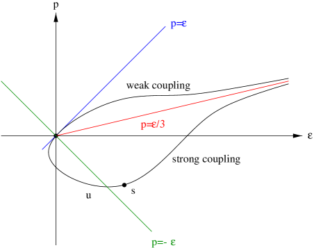
Figure 2: Change of form of the equation of state $p=f(\varepsilon,\varphi)$ in the model (4.1) as $\varphi$ varies from the weak-coupling region ($K(\varphi)>0$) to the strong-coupling one ($K(\varphi)<0$).

Let us investigate under what conditions on the functions $K(\varphi)$ and $L(\varphi)$ one can indeed approximately solve the master evolution equation (2.15) by considering that the variation of $\varphi$ brings only a small perturbation onto the simple $\varphi$-independent evolution studied above. We shall simplify this study by redefining the scalar field and working with the new field variable $\varphi^{\rm new}=\int d\varphi^{\rm old}L^{1/4}(\varphi^{\rm old})$ (which is well defined because we assume $L(\varphi)>0$). With this definition $L_{\rm new}(\varphi^{\rm new})=1$ and $K_{\rm new}(\varphi^{\rm new})=K_{\rm old}(\varphi^{\rm old})/L_{\rm old}^{1/2}(\varphi^{\rm old})$. In other words, we can assume, without loss of generality, that $L(\varphi)=1$. With this simplification the zeroth-order “slow-roll”, or “adiabatic”, solution to Eq. (2.15), i.e. the instantaneous attractive fixed point of Eq. (2.15) (solution of $0=\varepsilon+p=2X\partial p/\partial X)$ corresponds to

$$X_{\rm sr} = \frac{1}{2}\overline{K}(\varphi_{\rm sr}),$$ (4.6)

$$\dot{\varphi}_{\rm sr} = \sigma\sqrt{\overline{K}(\varphi_{\rm sr})},$$ (4.7)

$$\varepsilon_{\rm sr} = \frac{1}{4}\overline{K}^{2}(\varphi_{\rm sr}),$$ (4.8)

$$H_{\rm sr} = \frac{1}{2}\overline{K}(\varphi_{\rm sr}).$$ (4.9)

Here $\overline{K}(\varphi)\equiv-K(\varphi)$ is positive (in the slow-roll domain) and $\sigma$ denotes the sign of $\dot{\varphi}$. The time evolution of the slow-roll k-inflation is given, from Eqs. (4.6)-(4.9), by simple quadratures (the subscript “in” denotes initial values)

$$t-t_{\rm in} = \sigma\int_{\varphi_{\rm in}}^{\varphi}\frac{d\varphi}{\sqrt{\overline{K}(\varphi)}},$$ (4.10)

$$N \equiv \ln\left(\frac{a(t)}{a_{\rm in}}\right)=\frac{\sigma}{2}\int_{\varphi_{\rm in}}^{\varphi}\sqrt{\overline{K}(\varphi)}d\varphi.$$ (4.11)

[The notation $N$ is introduced to denote the number of $e$-folds of inflation.]

The post-slow-roll approximation, $X=X_{\rm sr}+\delta{X}$, is then obtained by rewriting the master equation (2.15) as

$$\frac{\partial p}{\partial X}=-\overline{K}+2X=2\delta X=-\frac{\dot{\varepsilon}}{6X\sqrt{\varepsilon}},$$ (4.12)

and replacing the slow-roll approximations (4.6)-(4.9) in the R.H.S. This yields

$$\frac{\delta X}{X_{\rm sr}}\simeq-\frac{1}{12}\frac{\dot{\varepsilon}}{\varepsilon^{3/2}}\simeq-\frac{\sigma}{3}\frac{\overline{K}^{\prime}}{\overline{K}^{3/2}}\simeq+\frac{2\sigma}{3}\left(\frac{1}{\sqrt{\overline{K}}}\right)^{\prime},$$ (4.13)

where the prime denotes a derivative with respect to $\varphi$. The criterion for the validity of our previous slow-roll solution (4.6)-(4.9) is

$$\frac{\delta X}{X}\ll 1,$$ (4.14)

i.e. $(\overline{K}^{-1/2})^{\prime}\ll 3/2$ (when keeping $L(\varphi)\neq 1$ it would read $L^{-1/4}\partial(L^{1/4}\overline{K}^{-1/2})$ $/\partial\varphi\ll 3/2$). This condition is as easily satisfied as the usual slow-roll condition for potential driven inflation. Examples of functions $\overline{K}(\varphi)$ that satisfy this condition are: (i) any power law or exponential (or super-exponential) growth as $\varphi\rightarrow\infty$, (ii) any levelling off of $\overline{K}(\varphi)$ ($\overline{K}(\varphi)\rightarrow{\rm limit}$, with $\overline{K}^{\prime}(\varphi)\rightarrow 0$) as $\varphi\rightarrow\infty$, or (iii) a sufficiently fast pole-like growth of $\overline{K}(\varphi)\propto(\varphi_{*}-\varphi)^{-\alpha}$, with $\alpha>2$, as $\varphi\rightarrow\varphi_{*}$.

Note that during slow-roll k-inflation the following useful relation

$$\frac{\varepsilon+p}{\varepsilon}\simeq 4\frac{\delta X}{X_{\rm sr}},$$ (4.15)

is satisfied, that is, the fractional compensation of the energy density by the negative pressure is proportional to the small parameter $\delta X/X_{sr}.$ Therefore, in those models where $\varepsilon+p>0,$ or equivalently, the energy density decreases in the course of expansion, $\delta X$ is positive. It is also obvious from (4.15), that inflation ends when $\delta X/X_{\rm sr}$ becomes of the order of unity, i.e. when the slow-roll condition (4.14) is violated.

For any function $\overline{K}(\varphi)$ (and more generally for any $p(\varphi,X)$) satisfying the slow-roll criterion we can visualize our k-inflationary behaviour as being one point (i.e. one value of $X=X_{\rm sr}+\delta X$) on an adiabatically varying equation of state graph of the type of Figs. 1 or 2. [The adiabatic variation we mention corresponding to the fact that each graph corresponds to some specific, instantaneous value of $\varphi$ , which is itself evolving]. Eq. (4.13) (or its generalization to a generic $p(\varphi,X)$) then tells us that the point $X=X_{\rm sr}+\delta X$ is always displaced away from the intersections of the ($\varphi$-instantaneous) graph with the $p=-\varepsilon$ line.

Overall, the qualitative behaviour of the solutions we are focussing on is the following: Initially, we start with some representative point in the $(\varepsilon,p)$ plane lying on an equation of state graph corresponding to some initial value of $\varphi$, deep into the strong coupling domain. We assume that, for strong coupling, the slow-roll criterion is very well satisfied. In a first evolution stage, we can neglect the $\varphi$-dependence of the equation of state because there is a fast attraction taking just a few $e$-folds of the representative point toward the nearest inflationary attractor (this stage is described by the arrows in Fig. 1). After this initial stage, we can consider that our representative point follows the (post-) slow-roll motion $X=X_{\rm sr}+\delta X$, corresponding to a representative point near but away from the $p=-\varepsilon$ line (such a point is indicated in Fig. 2). As the evolution continues, the slow-roll condition is less and less well satisfied and the representative point straggles more and more away from the $p=-\varepsilon$ line. At some point in the evolution the slow-roll criterion (4.14) becomes violated ($\delta X/X\sim 1$) and one naturally exits the inflationary stage. We shall come back later to this exit mechanism.

The qualitative picture of the evolution just represented (based on a succession of graphs in the $(\varepsilon,p)$ plane) can also be globally visualized by a phase-space picture in the $(\varphi,\dot{\varphi})$ plane (see Fig. 3). “Slow-roll” inflation on this graph corresponds to the portion of the separatrix (attractor) given by

$$\dot{\varphi}=\sigma\sqrt{\stackrel{{\scriptstyle\_}}{{K}}}\left(1+\frac{\delta X}{X_{\rm sr}}+...\right)^{1/2},$$ (4.16)

where $\delta X/X\ll 1.$ When $\delta X/X$ becomes of the order of one a graceful exit from inflation takes place, see Section VII. The phase diagram Fig. 3 is very similar to the one of potential driven slow-roll inflation [9]. We see that the set of initial configurations of the scalar field which lead to inflation has nonzero measure. Therefore the problem of initial conditions here is very similar to what one has in the case of chaotic inflation [1]. We expect that in analogy to the other models of inflation self-reproduction of the Universe [10] can take place in our k-inflationary model. However this question needs a special investigation and we leave it to future work.

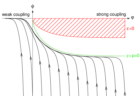
Figure 3: Schematic phase diagram of “slow-roll” $k$-inflation. Trajectories approach the attractor but do not reach the line $\epsilon+p=0$ where the speed of sound vanishes. Around the point where the slow-roll condition is violated, the solutions leave the inflationary stage and approach then smoothly the vacuum $\dot{\varphi}=0$.

Let us also mention that one can easily build a model in which one starts initially in the weak coupling regime, with the field $\varphi$ evolving towards the strong coupling regime. The function $K$ can then be arranged in such a way that the Universe leaves the weak coupling regime to enter an inflationary stage and finally exits inflation.

V “Power Law” k-Inflation

It is well known that, in the usual potential driven inflationary scenario, if the potential depends exponentially on the scalar field, there exists an attractor solution which describes a power law inflating Universe (see for instance [11]). There is no graceful exit from inflation if the potential is exponential everywhere. Therefore to solve the graceful exit problem one should assume that the exponential potential is a valid approximation of a more realistic and complicated potential only within some limited range of values of the scalar field $\varphi$. As we show in this section, one can get an analogous power law k-inflation within the class of models which we consider in this paper.

Let us again consider the model with the Lagrangian (4.1). For the purposes of this section it is convenient to make a new field redefinition (valid only in the region where $K<0$) and rewrite the Lagrangian (4.1) in terms of the new field variable $\varphi^{\rm new}=\int\sqrt{L(\varphi^{\rm old})/|K(\varphi^{\rm old})|}\,d\varphi^{\rm old}$. This yields

$$p=f\left(\varphi\right)\left(-X+X^{2}\right),$$ (5.1)

where $f\left(\varphi\right)\equiv f(\varphi^{\rm new})=K^{2}(\varphi^{\rm old})/L(\varphi^{\rm old})$ and $X\equiv X^{\rm new}=(L/|K|)X^{\rm old}$.

Working with this Lagrangian one can try to find out whether there is a function $f\left(\varphi\right)$ for which the master equation (2.15) has an exact solution which describes power law inflation. In the case of power law inflation

$$\varepsilon+p=\gamma\varepsilon,$$ (5.2)

where $\gamma$ is a constant. Substituting $\varepsilon$ and $p$ into the last equation we find immediately that if a solution exists, then

$$X=X_{0}=\frac{2-\gamma}{4-3\gamma}=const.$$ (5.3)

Expressing $\varepsilon$ in terms of $p$ from (5.2) and substituting (5.1) with $X$ given by (5.3) into the master Eq. (2.15), we get a simple equation for $f$, which is solved by

$$f\left(\varphi\right)=\frac{4}{9}\frac{\left(4-3\gamma\right)}{\gamma^{2}}\frac{1}{\left(\varphi-\varphi_{*}\right)^{2}}.$$ (5.4)

Therefore, a model with Lagrangian (5.1), with $f\left(\varphi\right)$ given by Eq. (5.4), has an attractor solution which describes power law expansion,

$$a\left(t\right)\varpropto t^{\frac{2}{3\gamma}}.$$ (5.5)

If $0<\gamma<2/3$ then this solution describes the usual power law inflation. If one takes a negative value of $\gamma$ then one gets pole-like super-inflation in Einstein frame. However, this pole-like inflation has a “graceful exit problem” which is very similar to the one of the pre-big bang scenario [2]. We were unable to find a simple solution to this problem and we doubt that such a solution can be meaningfully discussed within the effective field Lagrangian formalism considered here. Therefore we think that pole-like inflation does not help toward bringing a solution of the main cosmological problems. In distinction from pole-like inflation, in the model of power law inflation the graceful exit problem can be easily solved if in some range of $\varphi$ the function $f$ is modified in an obvious way.

A natural generalization of the Lagrangian (5.1),

$$p=f\left(\varphi\right)g\left(X\right),$$ (5.6)

where $g$ is a rather arbitrary function of $X$, opens the possibility to realize power law inflation in a wide class of theories. Actually, taking the function $f$ to be

$$f\left(\varphi\right)=-\frac{4}{9}\frac{\left(1-\gamma\right)}{\gamma^{2}}\frac{2X_{0}}{g\left(X_{0}\right)}\frac{1}{\left(\varphi-\varphi_{*}\right)^{2}},$$ (5.7)

where $X_{0}$ is a solution of the equation

$$2X\frac{\partial\ln g}{\partial X}=\frac{\gamma}{\gamma-1},$$ (5.8)

one can easily verify that power law inflation (5.5) is a solution of the corresponding theory.

VI Stability

A detailed study of the spectrum of quantum perturbations in our slow-roll k-inflation scenario will be done in a forthcoming publication. We shall only discuss here a necessary condition for the stability of our models with respect to arbitrary, high-frequency scalar perturbations. The equation for the canonical “quantization variable” $v$ describing the collective metric and scalar field perturbations in the case of the action (2.1) can be written down in the standard way [6] and takes the form [12]

$$v^{\prime\prime}-c_{s}^{2}\nabla^{2}v-\frac{z^{\prime\prime}}{z}v=0,$$ (6.1)

where the only relevant piece of information for our stability analysis is the appearance of the “speed of sound”

$$c_{s}^{2}=\frac{p_{,X}}{\varepsilon_{,X}}=\frac{p_{,X}}{p_{,X}+2Xp_{,XX}}$$ (6.2)

in front of the Laplacian. Here a comma denotes a partial derivative with respect to $X.$ It is clear that if $c_{s}^{2}$ is negative then the model is absolutely unstable. The increment of instability is inversely proportional to the wavelength of the perturbations, and therefore the background models for which $c_{s}^{2}<0$ are violently unstable and do not have any physical significance.

This stability requirement ($c_{s}^{2}=p_{,X}/\varepsilon_{,X}>0$) is non trivial within our scenario, because, for instance, in slow-roll k-inflation in the zeroth-order slow-roll approximation the inflationary attractors are defined by $p_{,X}=0$, and therefore $c_{s}^{2}=0$. However, as discussed in Section IV, in the post-slow-roll approximation, with $X=X_{\rm sr}+\delta X$, $p_{,X}$ does not vanish. To first order in $\delta X$ we can write $p_{,X}\simeq p_{,XX}^{\rm sr}\delta X$. Using the second equation (6.2) we get

$$c_{s}^{2}\simeq\frac{\delta X}{2X_{\rm sr}}.$$ (6.3)

Therefore stability requires that $\delta X>0$, i.e. that on the equation of state graphs of Figs. 1 and 2, the $\varphi$-gradients of $p(\varphi,X)$ be such that they displace the real, non-adiabatic, slow-roll attractor beyond the $p=-\varepsilon$ line (“beyond” meaning here “further away” as one runs along the $p=f(\varepsilon,\varphi)$ graph following the natural $X$ parametrization). These stable stretches of the $(\varepsilon,p)$ graphs are labelled $s$ in Fig. 1. They are also the stretches where the slope $(dp/d\varepsilon)$ is positive (as is clear from Eq. (6.2) which says that the velocity of sound is given by the usual formula $c_{s}^{2}=dp/d\varepsilon$, when keeping $\varphi$ fixed).

Let us now discuss the simple model (4.1). For this model we have computed $\delta X/X_{\rm sr}$, and we can therefore assess under what conditions k-inflation will be stable under scalar perturbations. We see from Eq. (4.13) that the conditions can be expressed in two (equivalent) forms: (i) the energy density $\varepsilon=\sqrt{\overline{K}}$ must decrease during the slow-roll of $\varphi$, or (ii) $-\sigma\overline{K}_{,\varphi}=\sigma K_{,\varphi}$ must be positive. The satisfaction of this condition is very natural within the intuitive picture we have in mind: namely, starting at some high ($\sim$ Planckian) energy density, i.e. a large negative value of $K(\varphi)=-\varepsilon^{2}$, and then letting $\varphi$ evolve toward the weak-field coupling domain where $K(\varphi)$ vanishes before becoming positive. During the slow-roll phase (with $K(\varphi)<0$), it is natural (and even necessary if $K(\varphi)$ is monotonic) to have a decreasing $\overline{K}=-K$.

One consequence applicable to a general model $p(\varphi,X)$ is that slow-roll implies a small value $|c_{s}^{2}|\ll 1$. It is interesting to ask for which (non slow-roll) models one can have both a continued k-inflation and a constant speed of sound of order unity. Let us consider for that purpose power law inflation. In the case where the Lagrangian takes the form (5.1) the speed of sound during the inflationary stage is

$$c_{s}^{2}=\frac{\gamma}{8-3\gamma}.$$ (6.4)

If we restrict ourselves to the inflationary range $0<\gamma<2/3$ this speed can not exceed $c_{s}^{2}=1/9.$ The smaller values of $\gamma$ correspond to very fast (nearly exponential) expansion and small speed of sound in complete agreement with our analysis of slow-roll k-inflation. Pole-like inflation is violently unstable in this model.

However, if we consider more general Lagrangians (5.6) we can avoid these restrictions. Actually in this case the speed of sound during the inflationary stage is given by the expression

$$c_{s}^{2}=\frac{g_{,X}\left(X_{0}\right)}{g_{,X}\left(X_{0}\right)+2X_{0}\,g_{,XX}\left(X_{0}\right)},$$ (6.5)

where $X_{0}$ is the solution of equation (5.8). The necessary conditions for power law inflation given in Section V imply that $g_{,X}\left(X_{0}\right)\not=0$ and do not involve any restrictions on the second derivative $g_{,XX}\left(X_{0}\right)$. Therefore, for a power law inflationary stage with any a priori given value of the parameter $\gamma$, one can always find a corresponding function $g\left(X\right)$ to arrange any required speed of sound. Note that it follows from here that one can also easily build a theory with pole-like inflation which is stable with respect to scalar perturbations.

VII Exit Mechanisms

In the simple model of Section IV (and in the normalization $L(\varphi)=1$) the total number of inflationary $e$-folds is (considering for definiteness that $\varphi$ decreases during slow-roll)

$$N_{\rm inf}=\frac{1}{2}\int\limits_{\varphi_{\rm end}}^{\varphi_{\rm in}}\sqrt{\overline{K}(\varphi)}\,d\varphi.$$ (7.1)

Here $\varphi_{\rm in}$ is the initial value of $\varphi$, and $\varphi_{\rm end}$ the end of slow-roll, i.e. the value of $\varphi$ where $\delta X/X$ becomes of order unity, i.e. (from Eq. (4.13)), such that

$$\overline{K}^{-3/2}(\varphi_{\rm end})\overline{K}^{\prime}(\varphi_{\rm end})\sim 1.$$ (7.2)

We shall not investigate here the problem of the choice of initial conditions within our model. We shall assume that some large parameter is present (or at least possible) in the problem and allows $N_{\rm inf}$ to be larger that 60 or so. [One simple possibility would be a function $K(\varphi)$ of the type of Eq. (4.3) which levels off to a negative constant when $\varphi$ increases. All the couples $(\varphi,X)$ where $X\sim 1$ (in Planck units) and $\varphi$ is arbitrary large lead to an energy density of order $1$. A random initial condition with $\varepsilon(\varphi_{\rm in},X_{\rm in})\sim 1$ could have an arbitrary large $\varphi$.] Assuming this we note not only that our mechanism contains a natural exit from inflation (because of the evolution of $K$ and its final change of sign), but that this exit is generically expected to take place within a small number of $e$-folds. Indeed, condition (7.2) signalling the end of slow-roll k-inflation can be rewritten (using Eqs. (4.6)-(4.9)) as $[\dot{K}/(KH)]_{\rm end}\sim 1$, which means that $K$ changes by 100% in a Hubble time, around the time of exit of k-inflation. One therefore expects that one can approximately match slow-roll k-inflation with a post-inflationary phase where $K(\varphi)$ has become positive.

We think that, in most cases, this way of exiting k-inflation provides a naturally graceful exit. Indeed, it is clear from Fig. 2 that, after the transition to the $K>0$ (“weak-coupling”) branch, the cosmological evolution will quickly be attracted toward an approximate $p\approx\varepsilon$ equation of state. The corresponding expansion was discussed in Eq. (3.2) and corresponds to a very fast decrease of the energy density: $\varepsilon_{\varphi}\propto a^{-6}$. As this decrease is much faster than the decay of the energy density in radiation ($\varepsilon_{\rm rad}\propto a^{-4}$) [and in non relativistic matter ($\varepsilon_{\rm matter}\propto a^{-3}$) if any is present], even small traces of the latter forms of energy present at the end of k-inflation will ultimately dominate the expansion. The situation is very similar to what has been recently discussed in Ref. [7]. As we have in mind that, in our model, the scalar $\varphi$ could be the dilaton (or a moduli), i.e. a field which modifies the coupling constants of all the other matter fields, we expect that the nearly uniform time variation of $\varphi$ during k-inflation will generate quantum particles at a uniform spacetime rate. During k-inflation the produced particles are constantly diluted by the fast expansion and are not expected to cause a strong back reaction, but the particles produced in the last $e$-fold of k-inflation should be sufficiently numerous to dominate soon the expansion. Even without this assumption (that the couplings of $\varphi$ are efficient in producing particles), the mere effect of the variable gravitational coupling (at the end of inflation) is sufficient to create any scalar particle with energy density (at birth) $\sim 10^{-2}H_{\rm end}^{4}$ [8] [4].

To discuss more precisely the evolution of the inflaton after it exits from k-inflation, i.e. when $K(\varphi)$ has become positive, and the higher-derivative term $L\,X^{2}$ has become negligible, it is convenient to introduce the canonical scalar field $\phi=\int d\varphi\sqrt{K(\varphi)}$. In terms of $\phi$ the equation of motion reads $\ddot{\phi}+3H\dot{\phi}=a^{-3}d(a^{3}\dot{\phi})/dt\approx 0$, with $H=\sqrt{\varepsilon_{\phi}+\varepsilon_{\rm rad}}$. Hence $a^{3}\dot{\phi}\simeq c=\mathrm{const}$ and $\phi$ evolves according to $\phi(t)\approx c\int dt\,a^{-3}$. In a first phase after k-inflation $\varepsilon_{\phi}$ probably dominates over $\varepsilon_{\rm rad}$ and the evolution follows the $p=\varepsilon$ attractor solution Eq. (3.2). During this initial phase $a(t)\propto t^{1/3}$ so that $\phi(t)$ drifts logarithmically: $\phi(t)\propto\int_{t_{\rm end}}^{t}dt/t=\ln(t/t_{\rm end})$. Later, $\varepsilon_{\rm rad}\propto a^{-4}$ will take over $\varepsilon_{\phi}\propto a^{-6}$ and the evolution will become radiation dominated. In this second phase, $a(t)\propto t^{1/2}$ and $\phi(t)\simeq c\int^{t}dta^{-3}\propto\int^{t}dt\,t^{-3/2}$ stops drifting logarithmically to converge toward some final value $\phi_{f}$: $\phi(t)\approx\phi_{f}-c^{\prime}t^{-1/2}$.

Note that, in this generic exit mechanism, the final value $\varphi_{f}$ of the original field (corresponding to the final value $\phi_{f}$ of the canonical field) is arbitrary. Therefore, if $\varphi$ is the dilaton or a moduli our k-inflationary mechanism does not, by itself, provide a mechanism for fixing $\varphi$ to a particular value. To do that one must appeal either to the presence, at low-energies, of a $\varphi$-dependent potential energy term $V(\varphi)$ (which may have been negligible at high energies), or to a non-trivial structure of couplings to matter [3]. We wish, however, to point out that some variants of our general model can also provide another way of fixing the end location of $\varphi$ very near a particular value. Indeed, if the kinetic function $K(\varphi)$ (of the original $\varphi$ variable) happens to have a pole singularity $K(\varphi)\propto(\varphi-\varphi_{p})^{-\alpha}$ with $\alpha\geq 2$ in the positive-$K$ domain the corresponding canonical field $\phi=\int d\varphi\sqrt{K(\varphi)}$ diverges when $\varphi\to\varphi_{p}$. Therefore, if this pole singularity is in the way of the evolution of $\varphi$ after the exit from k-inflation (e.g., if $\varphi_{p}<\varphi_{\rm end}<\varphi_{\rm in}$ in the case where $\dot{\varphi}<0$), the typically large logarithmic drift of the canonical field $\phi$ during the first phase after exit, $\Delta\phi\simeq c\int_{t_{\rm end}}^{t_{\rm rad}}dt\,a^{-3}\propto\ln(t_{\rm rad}/t_{\rm end})$ (where $t_{\rm rad}$ denotes the beginning of radiation domination), will mean that the original field $\varphi$ will end up very near $\varphi_{p}$.

Evidently, this mechanism assumes that, except for $K(\varphi)$, all the functions describing the coupling of $\varphi$ to matter (like the one giving the $\varphi$-dependence of the gauge couplings) are regular (or, at least, less singular) at $\varphi=\varphi_{p}$. Then, in the notation of Ref. [3], the observable coupling strength of $\varphi$ to matter $\alpha_{A}(\varphi)=d\ln m_{A}(\phi)/d\phi=(K(\varphi))^{-1/2}d\ln m_{A}(\varphi)/d\varphi$ is driven near zero by our mechanism.

VIII Conclusions

We have pointed out that a general class of higher-order scalar kinetic terms $p(\varphi,\nabla\varphi)=\frac{1}{2}K(\varphi)(\nabla\varphi)^{2}+\frac{1}{4}L(\varphi)(\nabla\varphi)^{4}+\cdots$ can drive an inflationary evolution starting from rather arbitrary initial conditions. Under not very restrictive conditions on the $\varphi$-dependence of the kinetic term $p(\varphi,\nabla\varphi)$ the early cosmological evolution will be attracted toward a slow-roll kinetically driven inflationary stage. In a large class of models this slow-roll behaviour has the following attractive features: (i) it drives the evolution from an initial high-curvature phase down to lower curvatures while dilating space in a quasi-exponential or power law manner, (ii) it is stable under (high-frequency) scalar perturbations, and (iii) it contains a natural exit mechanism because of the $\varphi$-dependence of the kinetic terms.

We have briefly discussed the exit of kinetically driven inflation and found that it seems to be naturally “graceful” in lending itself to a smooth transition toward a stage dominated by the radiation produced (either through the $\varphi$-dependence, or through purely gravitational effects) at the end of slow-roll. We have also pointed out that the presence of pole-like singularities in the $\varphi$-dependence of the kinetic terms can have some useful consequences: (i) a $\varphi$-dependence of the form $\sim(\varphi-\varphi_{*})^{-2}\tilde{p}(\nabla\varphi)$ in the initial field domain can ensure a nearly constant speed of sound of order unity, while (ii) a pole-like singularity in the coefficient $(\nabla\varphi)^{2}$ in the final field domain can help to fix the value of $\varphi$ to a specific value.

We leave to future work the investigation of general important issues: the choice of (a measure on the) initial conditions, and the computation of the perturbation spectra generated by this new type of inflation. We are aware that the compatibility of the latter issues with observations will probably necessitate the presence of some small (or large) dimensionless parameters in $p(\varphi,\nabla\varphi)$.

In this work, we have used the structure of the effective action in string theory as a partial motivation for considering higher-order kinetic terms $p(\varphi,\nabla\varphi)$. Having found that such terms can generically drive an inflationary behaviour, we hope that our mechanism might be useful in suggesting new ways in which the dilaton and moduli fields of string theory might be compatible with inflation.

References

- [1] For a review, see e.g., A. Linde, Particle Physics and Inflationary Cosmology, (1990) Harwood, N. J.
-
[2]
G. Veneziano, Phys. Lett. B265, 287 (1991)
M. Gasperini and G. Veneziano, Astropart. Phys. 1, 317 (1993)
For an updated collection of papers on the pre-big bang scenario see http://www.to.infn.it/~gasperin/ - [3] T. Damour and A. Polyakov, Nucl. Phys. B423, 532 (1994)
- [4] T. Damour and A. Vilenkin, Phys. Rev. D53, 298 (1996)
- [5] S. Foffa, M. Maggiore and R. Sturani, hep-th/9903008 and references therein.
- [6] V. Mukhanov, H. Feldman and R. Brandenberger, Phys. Rept. 215, 203 (1992)
- [7] P. Peebles and A. Vilenkin, astro-ph/9810509
- [8] L. Ford, Phys. Rev. D35, 2955 (1987)
- [9] V. Belinskii, L. Grischuk, Ya. Zel’dovich and I. Khalatnikov, Sov. Phys. JETP 62, 195 (1985)
- [10] A. Linde, D. Linde and A. Mezhlumian, Phys. Rev. D49, 1783 (1994)
- [11] F. Lucchin and S. Matarrese, Phys. Rev. D32, 1316 (1985)
- [12] J. Garriga and V. Mukhanov, In preparation.