UPR-843T, PUPT-1856
Moduli Spaces of Fivebranes on Elliptic Calabi-Yau Threefolds

We present a general method for calculating the moduli spaces of fivebranes wrapped on holomorphic curves in elliptically fibered Calabi–Yau threefolds, in particular, in the context of heterotic M theory. The cases of fivebranes wrapped purely on a fiber curve, purely on a curve in the base and, generically, on a curve with components both in the fiber and the base are each discussed in detail. The number of irreducible components of the fivebrane and their properties, such as their intersections and phase transitions in moduli space, follow from the analysis. Even though generic curves have a large number of moduli, we show that there are isolated curves that have no moduli associated with the Calabi–Yau threefold. We present several explicit examples, including cases which correspond to potentially realistic three family models with grand unified gauge group $SU(5)$.

1 Introduction

If string theory is to be a model of supersymmetric particle physics, one should be able to find four-dimensional vacua preserving $\mathcal{N}=1$ supersymmetry. The first examples of such backgrounds arose as geometrical vacua, from the compactification of the heterotic string on a Calabi–Yau threefold. Recent advances in string duality have provided new ways of obtaining geometrical $\mathcal{N}=1$ vacua, by compactifying other limits of string theory and, in particular, by including branes in the background.

Of particular interest is the strongly coupled limit of the $E_{8}\times E_{8}$ heterotic string. The low-energy effective theory is eleven-dimensional supergravity compactified on an $S^{1}/Z_{2}$ orbifold interval, with a set of $E_{8}$ gauge fields on each of the ten-dimensional orbifold fixed planes [1, 2]. To construct a theory with $\mathcal{N}=1$ supersymmetry one further compactifies on a Calabi–Yau threefold $X$ [3]. One is then free to choose general $E_{8}$ bundles which satisfy the hermitian Yang–Mills equations. Furthermore, one can include some number of five-branes. The requirements of four-dimensional Lorentz invariance and supersymmetry mean that these branes must span the four-dimensional Minkowski space, while the remaining two dimensions wrap a holomorphic curve within the Calabi–Yau threefold [3, 4, 5].

In the low-energy four-dimensional effective theory, there is an array of moduli. There are geometrical moduli describing the dimensions of the Calabi–Yau manifold and orbifold interval. There are bundle moduli describing the two $E_{8}$ gauge bundles. And finally, there are moduli describing the positions of the fivebranes. It is this last set of moduli, together with the generic low-energy gauge fields on the fivebranes, upon which we shall focus in this paper. We note that, although we consider this problem in the specific case of M fivebranes, the moduli spaces are quite general and should have applications to other supersymmetric brane configurations.

We shall look at this question in the particular case of an elliptically fibered Calabi–Yau threefold with section. This expands on the discussion of we gave in a recent letter [6]. There we used this special class of manifolds to construct explicitly an array of new particle physics vacua. The general structure of the constructions was given in detail in a second paper [7]. This is the companion paper which explains the structure of the five-brane moduli space as well as the nature of gauge enhancement on the five-branes.

The constructions in [6] and [7] used the analysis of gauge bundles on elliptic Calabi–Yau threefolds given by Friedman, Morgan and Witten [8], Donagi [9] and Bershadsky et al. [10]. The vacua preserved, for example, $SU(5)$ or $SO(10)$ gauge symmetry with three families. The presence of the five-branes allowed a much larger class of possible backgrounds. The number of families is given by an index first calculated in this context by Andreas [11] and Curio [12]. Curio also gave explicit examples of bundles where this index was three. Subsequently, the case of non-simply connected elliptic Calabi–Yau threefolds with bisections has been considered in [13]. We note that, in the M theory context, another class of explicit models with non-standard gauge bundles but with orbifold Calabi–Yau spaces, were first contructed in [14], while the generic form of the effective four- and five-dimensional theories, including fivebranes, is given in [15].

In constructing these vacua the fivebranes cannot be chosen arbitrarily [3]. The boundaries of $S^{1}/Z_{2}$ and the fivebranes are all magnetic sources for the four-form field strength $G$ of eleven-dimensional supergravity. The fact that there can be no net magnetic charge for $G$ in the Calabi–Yau threefold fixes the homology class of the fivebranes in terms of the gauge bundles and $X$ itself. As discussed in [6, 7], to describe real fivebranes this homology class must be “effective” in $X$. Mathematically, then, the problem we wish to solve is to find the moduli space of holomorphic curves in $X$ in a given effective homology class.

Specific to the M theory case, we will also include the moduli corresponding to moving the fivebranes in $S^{1}/Z_{2}$ and, in addition, their axionic moduli partners [15, 16, 17]. These latter fields are compact scalars which arise as zero modes of the self-dual three-form $h$ on the fivebranes. The other zero modes of $h$ lead to low-energy gauge fields. Generically the gauge group is $U(1)^{g}$, where $g$ is the genus of the holomorphic curve [15, 16, 17]. Since we will be able to calculate $g$ at each point in the moduli space, we will also be able to identify the low-energy gauge multiplets.

One consequence of considering elliptically fibered Calabi–Yau threefolds with section is that there is a dual F theory description [18, 19, 20]. For the fivebranes, those wrapping purely on the fiber of $X$ correspond to threebranes on the F theory side [8]. Rajesh [21] and Diaconescu and Rajesh [22] have recently argued that fivebranes lying wholly in the base of $X$ correspond to blow-ups of the corresponding curve in the F theory vacuum. We will not comment in detail on this interesting correspondence. However, we will show that, locally, the moduli spaces match those expected from duality to F theory. We will also comment on how the global structure is encoded on the M theory side through a twisting of the axion modulus. This will be discussed further in [23]. An additional point we will only touch on is the structure of additional low-energy fields which can appear when fivebranes intersect. We will, however, clearly identify these points in moduli space in our analysis. Finally, we will also ignore any non-perturbative corrections. In general, since the low-energy theory is only $\mathcal{N}=1$, one expects that some of the directions in moduli space are lifted by non-perturbative effects, in particular by instantonic membranes stretching between fivebranes.

Specifically, we do the following. In section 2, we briefly review the anomaly cancellation condition in heterotic M-theory, discuss how that constraint leads to non-perturbative vacua with fivebranes and review some aspects of homology and cohomology theory required in our analysis. Properties of elliptically fibered Calabi–Yau threefolds and a discussion of their algebraic and effective classes are presented in section 3. Section 4 is devoted to studying the simple case of the the moduli spaces of fivebranes wrapped purely on the elliptic fiber. We also comment on global structure of the moduli space and the relation to F theory. In section 5, we present two examples of fivebranes wrapping curves with a component in the base. We analyze, in detail, the moduli space of these two examples, including the generic low-energy gauge groups on and possible intersections of the fivebrane. Techniques developed in sections 4 and 5 are generalized in section 6, where we give a procedure for the analysis of the moduli spaces of fivebranes wrapped on any holomorphic curve, generically with both a fiber and a base component. We note a particular exceptional case which occurs when the fivebrane wraps an exceptional divisor in the base. Finally, in sections 7, 8 and 9 we make these methods concrete by presenting three specific examples, two with a del Pezzo base and one with a Hirzebruch base. Two of these examples correspond realistic three-family, non-perturbative vacua in Hořava-Witten theory.

2 Heterotic M theory vacua with fivebranes

2.1 Conditions for a supersymmetric background

As we have discussed in the introduction, the standard way to obtain heterotic vacua in four dimensions with $\mathcal{N}=1$ supersymmetry, is to compactify eleven-dimensional M theory on the manifold $X\times S^{1}/Z_{2}\times M_{4}$ [1, 2]. Here $X$ is a Calabi–Yau threefold, $S^{1}/Z_{2}$ is an orbifold interval, while $M_{4}$ is four-dimensional Minkowski space. This background is not an exact solution, but is good to first order in an expansion in the eleven-dimensional Planck length. To match to the low-energy particle physics parameters, the Calabi–Yau threefold is chosen to be the size of the Grand Unified scale, while the orbifold is somewhat larger [3, 24]. In general, there is a moduli space of different compactifications. There are the familiar moduli corresponding to varying the complex structure and the Kähler metric on the Calabi–Yau threefold. Similarly, one can vary the size of the orbifold. These parameters all appear as massless fields in the low-energy four-dimensional effective action. In general, there are additional low-energy scalar fields coming from zero-modes of the eleven-dimensional three-form field $C$.

The second ingredient required to specify a supersymmetric background is to choose the gauge bundle on the two orbifold planes. In general, one can turn on background gauge fields in the compact Calabi–Yau space. Supersymmetry implies that these fields cannot be arbitrary. Instead, they are required to satisfy the hermitian Yang–Mills equations

$$F_{ab}=F_{{\bar{a}}{\bar{b}}}=0\qquad g^{a{\bar{b}}}F_{a{\bar{b}}}=0$$ (2.1)

Here $a$ and $b$ are holomorphic indices in $X$, ${\bar{a}}$ and ${\bar{b}}$ are antiholomorphic indices, while $g_{a{\bar{b}}}$ is the Kähler metric on $X$. Having fixed the topology of the gauge bundle, that is, how the bundle is patched over the Calabi–Yau manifold, there is then a set of different solutions to these equations. There are additional low-energy moduli which interpolate between these different solutions. In general, the full moduli space of bundles is hard to analyze. However, when the Calabi–Yau threefold is elliptically fibered, the generic structure of this moduli space can be calculated and has been discussed in [8, 9] and also in [25].

The final ingredient to the background is that one can include fivebranes [3, 15]. In order to preserve supersymmetry and four-dimensional Lorentz invariance, the fivebranes must span the four-dimensional Minkowski space while the remaining two dimensions wrap a holomorphic curve within the Calabi–Yau threefold [3, 4, 5]. In addition, each brane must be parallel to the orbifold fixed planes. Thus it is localized at a single point in $S^{1}/Z_{2}$. Again, there are a set of moduli giving the positions of the five-branes within the Calabi–Yau manifold as well as in the orbifold interval. As we will discuss below, there are also extra moduli coming from the self-dual tensor fields on the fivebranes [15, 16, 17]. These fields generically give some effective $\mathcal{N}=1$ gauge theory in four-dimensions. Finding the moduli space of the fivebranes, and some information about the effective gauge theory which arises on the fivebrane worldvolumes will be the goal of this paper.

In summary, the M theory background is determined by choosing

• a spacetime manifold of the form $X\times S^{1}/Z_{2}\times M_{4}$, where $X$ is a Calabi–Yau threefold

• two $E_{8}$ gauge bundles, $V_{1}$ and $V_{2}$, satisfying the hermitian Yang–Mills equations (2.1) on $X$

• a set of fivebranes parallel to the orbifold fixed planes and wrapped on holomorphic curves within $X$.

This ensures that we preserve $\mathcal{N}=1$ supersymmetry in the low-energy four-dimensional effective theory.

2.2 Cohomology condition

The above conditions are not sufficient to ensure that one has a consistent background. Anomaly cancellation on both the ten-dimensional orbifold fixed planes and the six-dimensional fivebranes is possible only because each is a magnetic source for the supergravity four-form field strength $G=dC$ [3]. This provides an inflow mechanism to cancel the anomaly on the lower dimensional space. In general, the magnetic sources for $G$ are five-forms. Explicitly, if $0\leq x^{11}\leq\pi\rho$ parameterizes the orbifold interval, one has [15]

$$dG=J_{1}\wedge\delta(x^{11})+J_{2}\wedge\delta(x^{11}-\pi\rho)+\sum_{i}J_{5}^{(i)}\wedge\delta(x^{11}-x^{(i)})$$ (2.2)

where $J_{1}$ and $J_{2}$ are four-form sources on the two fixed planes and $J_{5}^{(i)}$ is a delta-function four-form source localized at the position of the $i$-th five-brane in $X$. The explicit one-form delta functions give the positions of the orbifold fixed planes at $x^{11}=0$ and $x^{11}=\pi\rho$ and the five-branes at $x^{11}=x^{(i)}$ in $S^{1}/Z_{2}$.

Compactifying on $X\times S^{1}/Z_{2}$, we have the requirement that the net charge in the internal space must vanish, since there is nowhere for flux to escape. Equivalently, the integral of $dG$ over any five-cycle in $X\times S^{1}/Z_{2}$ must be zero since $dG$ is exact. Integrating over the orbifold interval then implies that the integral of $J_{1}+J_{2}+\sum_{i}J_{5}^{(i)}$ over any four cycle in $X$ must vanish. Alternatively, this means that the sum of these four-forms must be zero up to an exact form, that is, they must vanish cohomologically.

Explicitly, the source on each orbifold plane is proportional to

$$J_{n}\sim\mathrm{tr}F_{n}\wedge F_{n}-\frac{1}{2}\mathrm{tr}R\wedge R$$ (2.3)

where $F_{n}$ for $n=1,2$ is the $E_{8}$ field strength on the $n$-th fixed plane, while $R$ is the spacetime curvature. The full cohomology condition can then be written as

$$\lambda(TX)=w(V_{1})+w(V_{2})+[W]$$ (2.4)

with

$$w(V) =-\frac{1}{60\cdot 8\pi^{2}}\mathrm{tr}_{\bf 248}F\wedge F$$ (2.5)

$$\lambda(TX) =\frac{1}{2}p_{1}(TX)=-\frac{1}{2\cdot 8\pi^{2}}\mathrm{tr}_{\bf 6}R\wedge R$$

where the right-hand sides of these expressions really represent cohomology classes, rather than the forms themselves. The traces are in the adjoint ${\bf 248}$ of $E_{8}$ and the vector representation of $SO(6)$. $[W]$ represents the total cohomology class of the five-branes, which we will discuss in a moment. Note that $\lambda$ is half the first Pontrjagin class. It is, in fact, an integer class because we are on a spin manifold. On a Calabi–Yau threefold it is equal to the second Chern class $c_{2}(TX)$, where the tangent bundle $TX$ is viewed as an $SU(3)$ bundle and the trace is in the fundamental representation. Thus, the cohomology condition simplifies to

$$[W]=c_{2}(TX)-w(V_{1})-w(V_{2})$$ (2.6)

What do we mean by the cohomology class $[W]$? We recall that we associated four-form delta function sources to the five-branes in $X$. The class $[W]$ is then the cohomology class of the sum of all these sources. Recall that the five-branes wrap on holomorphic curves within the Calabi–Yau threefold. The sum of the five-branes thus represents an integer homology class in $H_{2}(X,\mathbf{Z})$. In general, one can then use Poincaré duality to associate an integral cohomology class in $H^{4}(X,\mathbf{Z})$ to the homology class of the fivebranes, or also a de Rham class in $H_{\mathrm{DR}}^{4}(X,\mathbf{R})$. This is the class $[W]$ which enters the cohomology condition, though we will throughout use the same expression $[W]$ for the integral homology class in $H_{2}(X,\mathbf{Z})$, the integral cohomology class in $H^{4}(X,\mathbf{Z})$, and the de Rham cohomology class in $H_{\mathrm{DR}}^{4}(X,\mathbf{R})$.

2.3 Homology classes and effective curves

Let us now turn to analyzing the cohomology condition (2.6) in more detail. One finds that the requirement that $[W]$ correspond to the homology class of a set of supersymmetric fivebranes puts a constraint on the allowed bundle classes [6, 7].

Since the sources are all four-forms, equation (2.6) is clearly a relation between de Rahm cohomology classes $H_{\mathrm{DR}}^{4}(X,\mathbf{R})$. However, in fact, the sources are more restricted than this. In general, they are all in integral cohomology classes. By this we mean that their integral over any four-cycle in the Calabi–Yau threefold gives an integer. (As noted above, this is even true when we no longer have a Calabi–Yau threefold but only a spin manifold, and $c_{2}(TX)$ is replaced by $\frac{1}{2}p_{1}(X)$.) The class $[W]$ is integral because it is Poincaré dual to an integer sum of fivebranes, an element of $H_{2}(X,\mathbf{Z})$. Note that there is a general notion of the integer cohomology group $H^{p}(X,\mathbf{Z})$ which, in general, includes discrete torsion groups such as $\mathbf{Z}_{2}$. This maps naturally to de Rahm cohomology $H_{\mathrm{DR}}^{p}(X,\mathbf{R})$. However, it is important to note that the map is not injective. Torsion elements in $H^{p}(X,\mathbf{Z})$ are lost. The integral classes to which we refer in this paper are to be identified with the images of $H^{p}(X,\mathbf{Z})$ in $H_{\mathrm{DR}}^{p}(X,\mathbf{R})$.

In general, $[W]$ cannot be just any integral class. We have seen that supersymmetry implies that fivebranes are wrapped on holomorphic curves within $X$. Thus $[W]$ must correspond to the homology class of holomorphic curves. Furthermore, $[W]$ must refer to some physical collection of fivebranes. Included in $H_{2}(X,\mathbf{Z})$ are negative classes like $-[C]$ where $C$ is, for example, a holomorphic curve in $X$. These have cohomology representatives which would correspond to the “absence” of a five-brane, contributing a negative magnetic charge to the Bianchi identity for $G$ and negative stress-energy. Such states are physically not allowed. The condition that $[W]$ describes physical, holomorphic fivebranes further constrains $c_{2}(TX)$, $w(V_{1})$ and $w(V_{2})$ in the cohomology condition (2.6).

In order to formalize these constraints, we need to introduce some definitions. We will use the following terminology.

• A curve is a holomorphic complex curve in the Calabi–Yau manifold. A curve is reducible if it can be written as the union of two curves.

• A class is a homology class in $H_{2}(X,\mathbf{Z})$ (or the Poincaré dual cohomology class in $H^{4}(X,\mathbf{Z})$). In general, it may or may not have a representative which is a holomorphic curve. If it does, then a class is irreducible if it has an irreducible representative. Note that there may be other curves in the class which are reducible, but the class is irreducible if there is at least one irreducible representative.

• A class which can be written as a sum of irreducible classes with arbitrary integer coefficients is called algebraic.

• A class is effective if it can be written as the sum of irreducible classes with positive integer coefficients.

Note that we will occasionally use analogous terminology to refer to surfaces (or divisors) in $X$. These are holomorphic complex surfaces in the Calabi–Yau threefold, so they have four real dimensions, and their classes lie in $H_{4}(X,\mathbf{Z})$.

Physically, the above definitions correspond to the following. A curve $W$ describes a collection of supersymmetric fivebranes wrapped on holomorphic two-cycles in the Calabi–Yau space. A reducible curve is the union of two or more separate five-branes. A general class in $H_{2}(X,\mathbf{Z})$ has representatives which are a general collection of five-branes, perhaps supersymmetric, perhaps not, and maybe including “negative” fivebranes of the form mentioned above. An algebraic class, on the other hand, has representatives which are a collection of only five-branes wrapped on holomorphic curves and so supersymmetric, but again includes the possibility of negative fivebranes. Finally, an effective class has representatives which are collections of supersymmetric fivebranes but exclude the possibility of non-physical negative fivebrane states.

From these conditions, we see that the constraint on $[W]$ is that we must choose the Calabi–Yau threefold and the gauge bundles $V_{1}$ and $V_{2}$ such that

$$[W]$$ must be effective (2.7)

As it stands, it is not clear that $[W]=c_{2}(TX)-w(V_{1})-w(V_{2})$ is algebraic, let alone effective. However, supersymmetry implies that both the tangent bundle and the gauge bundles are holomorphic. There is then a useful theorem that the classes of holomorphic bundles are algebraic, and so $[W]$ is in fact necessarily algebraic. However, there remains the condition that $[W]$ must be effective which does indeed constrain the allowed gauge bundles on a given Calabi–Yau threefold.

2.4 The theory on the fivebranes, $\mathcal{N}=1$ gauge theories and the fivebrane moduli space

While two of the fivebrane dimensions are wrapped on a curve within the Calabi–Yau manifold, the remaining four dimensions span uncompactified Minkowski space. The low-energy massless degrees of freedom on a given fivebrane consequently fall into four-dimensional $\mathcal{N}=1$ multiplets. At a general point in moduli space there are a set of complex moduli $(m_{i},\bar{m}_{i})$ describing how the fivebrane curve can be deformed within the Calabi–Yau three-fold. These form a set of chiral multiplets. In addition, there is a single real modulus $x^{11}$ describing the position of the fivebrane in the orbifold interval. This is paired under supersymmetry with an axion $a$ which comes from the reduction of the self-dual three-form degree of freedom, $h$, on the fivebrane to form a further chiral multiplet. When the fivebrane is non-singular, that is, does not intersect itself, touch another fivebrane, or pinch, at any point, the remaining degrees of freedom are a set of $U(1)$ gauge multiplets, where the gauge fields also arise from the reduction of the self-dual three-form. The number of $U(1)$ fields is given by the genus $g$ of the curve. In summary, generically, we have

chiral multiplets: $$\quad(x^{11},a),\,(m_{i},\bar{m}_{i})$$ (2.8)

vector multiplets:    $$g U(1)^{g}$$ multiplets with gauge group

for each distinct fivebrane.

When the fivebrane becomes singular, new degrees of freedom can appear. These correspond to membranes stretched between parts of the same fivebrane, or the fivebrane and other fivebranes, which shrink and become massless when the fivebrane becomes singular. They may be new chiral or vector multiplets. In the following, we will not generally identify all the massless degrees of freedom at singular configurations but, rather, concentrate on describing the degrees of freedom on the smooth parts of the moduli space.

In conclusion, we have seen that fixing the Calabi–Yau manifold and gauge bundles, in general, fixes an element $[W]$ of $H_{2}(X,\mathbf{Z})$ describing the homology class of the holomorphic curve in $X$ on which the fivebranes are wrapped. In order to describe an actual set of fivebranes, $[W]$ must be effective, which puts a constraint on the choice of gauge bundles. In general, there are a great many different arrangements of fivebranes in the same homology class. The fivebranes could move about within the Calabi–Yau threefold and also in the orbifold interval. In addition, there can be transitions where branes split and join. The net effect is that there is, in general, a complicated moduli space of five-branes parameterizing all the different possible combinations. In the low-energy effective theory on the fivebranes, the moduli space is described by a set of chiral multiplets. In order to describe the structure of this moduli space, it is clear that we need to analyze the moduli space of all the holomorphic curves in the class $[W]$, including the possibility that each fivebrane can move in $S^{1}/Z_{2}$ and can have a different value of the axionic scalar $a$.

3 Elliptically fibered Calabi–Yau manifolds

The moduli spaces we will investigate in detail in this paper are those for five-branes wrapped on smooth elliptically fibered Calabi–Yau threefolds $X$. Consequently, in this section we will briefly summarize the structure of $X$, then identify the generic algebraic classes and finally understand the conditions for these classes to be effective.

3.1 Properties of elliptically fibered Calabi–Yau threefolds

An elliptically fibered Calabi–Yau threefold $X$ consists of a base $B$, which is a complex surface, and an analytic map

$$\pi:X\to B$$ (3.1)

with the property that for a generic point $b\in B$, the fiber $E_{b}=\pi^{-1}(b)$ is an elliptic curve. That is, $E_{b}$ is a Riemann surface of genus one with a particular point, the origin $p$, identified. In particular, we will require that there exist a global section, denoted $\sigma$, defined to be an analytic map

$$\sigma:B\to X$$ (3.2)

that assigns to every point $b\in B$ the origin $\sigma(b)=p\in E_{b}$. We will sometimes refer to this as the zero section. The requirement that the elliptic fibration have a section is crucial for duality to F theory. However, one notes that from the M theory point of view it is not necessary.

In order to be a Calabi–Yau threefold, the canonical bundle of $X$ must be trivial. From the adjunction formula, this implies that the normal bundle to the section, $N_{B/X}$, which is a line bundle over $B$ and tells us how the elliptic fiber twists as one moves around the base, must be related to the canonical bundle of the base, $K_{B}$. In fact,

$$N_{B/X}=K_{B}.$$ (3.3)

Further conditions appear if one requires that the Calabi–Yau threefold be smooth. The canonical bundle $K_{B}$ is then constrained so that the only possibilities for the base manifold are as follows [20, 27]:

• for a smooth Calabi–Yau manifold the base $B$ can be a del Pezzo ($dP_{r}$), Hirzebruch ($F_{r}$) or Enriques surface, or a blow-up of a Hirzebruch surface.

These are the only possibilities we will consider. The structure of these surfaces is discussed in detail in an appendix to [7]. In the following, we will adopt the notation used there.

It will be useful to recall that, in general, there is a set of points in the base at which the fibration becomes singular. These form a curve, the discriminant curve $\Delta$, which is in the homology class $-12K_{B}$, as can be shown explicitly by considering the Weierstrass form of the fibration.

3.2 Algebraic classes on $X$

Since $[W]$ is algebraic, we need to identify the set of algebraic classes on our elliptically fibered Calabi–Yau manifold. This was discussed in [6, 7], but here we will be more explicit. It will be useful to identify these classes both in $H_{2}(X,\mathbf{Z})$ and $H_{4}(X,\mathbf{Z})$. In general, the full set of classes will depend on the particular fibration in question. However, there is a generic set of classes which are always present, independent of the fibration, and this is what we will concentrate on.

Simply because we have an elliptic fibration, the fiber at any given point is a holomorphic curve in $X$. Consequently, one algebraic class in $H_{2}(X,\mathbf{Z})$ which is always present is the class of the fiber, which we will call $F$. The existence of a section means there is also a holomorphic surface in $X$. Thus the class of the section, which we will call $D$, defines an algebraic class in $H_{4}(X,\mathbf{Z})$.

Some additional algebraic classes may be inherited from the base $B$. In general, $B$ has a set of algebraic classes in $H_{2}(B,\mathbf{Z})$. One useful fact is that for all the bases which lead to smooth Calabi–Yau manifolds, one finds that every class in $H_{2}(B,\mathbf{Z})$ is algebraic. This follows from the Lefschetz theorem [26] which tells us that we can identify algebraic classes on a surface $S$ with the image of integer classes in the Dolbeault cohomology $H^{1,1}(S)$. One then has the following picture. In general, the image of $H^{2}(S,\mathbf{Z})$ is a lattice of points in $H^{2}(S,\mathbf{R})$. Choosing a complex structure on $S$ corresponds to fixing an $h^{1,1}$-dimensional subspace within $H^{2}(S,\mathbf{R})$ describing the space $H^{1,1}(S)$. Generically, no lattice points will intersect the subspace and so there are no algebraic classes on $S$. The exception is when $h^{2,0}=0$, which is the case for all the possible bases $B$. Then the subspace is the whole space $H^{2}(S,\mathbf{R})$ so all classes in $H^{2}(S,\mathbf{Z})$ are algebraic.

If $\Omega$ is an algebraic class in $H_{2}(B,\mathbf{Z})$, there are two ways it can lead to a class in $X$. First, one can use the section $\sigma$ to form a class in $H_{2}(X,\mathbf{Z})$. If $C$ is some representative of $\Omega$, then the inclusion map $\sigma$ gives a curve $\sigma(C)$ in $X$. The homology class of this curve in $H_{2}(X,\mathbf{Z})$ is denoted by $\sigma_{*}\Omega$. Second, we can use the projection map $\pi$ to pull $\Omega$ back to a class in $H_{4}(X,\mathbf{Z})$. For a given representative $C$, one forms the fibered surface $\pi^{-1}(C)$ over $C$. The homology class of this surface in $H_{4}(X,\mathbf{Z})$ is then denoted by $\pi^{*}\Omega$. This structure is indicated in Figure 1.

Figure 1: Generic algebraic classes on $X$, where $[C]=\sigma_{*}\Omega$ and the fiber class $[E_{p}]=F$ are in $H_{2}(X,\mathbf{Z})$, and $[\pi^{-1}(C)]=\pi^{*}\Omega$ and base class $[B]=D$ are in $H_{4}(X,\mathbf{Z})$.

In general, these maps may have kernels. For instance, two curves which are non-homologous in $B$, might be homologous once one embeds them in the full Calabi–Yau threefold. In fact, we will see that this is not the case. One way to show this, which will be useful in the following, is to calculate the intersection numbers between the classes in $H_{2}$ and $H_{4}$. We find

$$\begin{array}[]{rrccc}&&&\lx@intercol\hfil H_{2}(X,\mathbf{Z})\hfil\lx@intercol\\ &&\vline&\sigma_{*}\Omega^{\prime}&F\\ \cline{2-5}\cr H_{4}(X,\mathbf{Z})&\begin{array}[]{c}\pi^{*}\Omega\\ D\end{array}&\vline&\begin{array}[]{c}\Omega\cdot\Omega^{\prime}\\ K_{B}\cdot\Omega^{\prime}\end{array}&\begin{array}[]{c}0\\ 1\end{array}\end{array}$$ (3.4)

where the entries in the first column are the intersections of classes in $B$. The intersection of $\sigma_{*}\Omega^{\prime}$ with $D$ is derived by adjunction, recalling that the normal bundle to $B$ is $N_{B/X}=K_{B}^{-1}$. Two classes are equivalent if they have the same intersection numbers. If we take a set of classes $\Omega_{i}$ which from a basis of $H_{2}(B,\mathbf{Z})$, we see that the matrix of intersection numbers of the form given in (3.4) is non-degenerate. Thus, for each nonzero $\Omega\in H_{2}(B,\mathbf{Z})$, we get nonzero classes $\sigma_{*}\Omega$ and $\pi^{*}\Omega$ in $H_{2}(X,\mathbf{Z})$ and $H_{4}(X,\mathbf{Z})$.

As we mentioned, the algebraic classes we have identified so far are generic, always present independently of the exact form of the fibration. There are two obvious sources of additional classes. Consider $H_{4}(X,\mathbf{Z})$. First, we could have additional sections non-homologous to the zero-section $\sigma$. Second, the pull-backs of irreducible classes on $B$ could split so that $\pi^{*}(\Omega)=\Sigma_{1}+\Sigma_{2}$. This splitting comes from the fact that there can be curves on the base over which the elliptic curve degenerates, for example, into a pair of spheres. New classes appear from wrapping the four-cycle over either one sphere or the other. Now consider $H_{2}(X,\mathbf{Z})$. We see that the possibility of degeneration of the fiber means that the fiber class $F$ can similarly split, with representatives wrapped, for instance, on one sphere or the other. Finally, the presence of new sections means there is a new way to map curves from $B$ into $X$ and, in general, classes in $H_{2}(B,\mathbf{Z})$ will map under the new section to new classes in $H_{2}(X,\mathbf{Z})$.

In all our discussions in this paper, we will ignore these additional classes. This will mean that our moduli space discussion is not in general complete. However, this restriction will allow us to analyze generic properties of the moduli space. In summary, we have identified the generic algebraic classes $\Omega$ in $H_{2}(X,\mathbf{Z})$ as classes in $B$ (since these are all algebraic for the bases in question) mapped via the section into $X$, together with the fiber class $F$; while in $H_{4}(X,\mathbf{Z})$ the generic algebraic classes are the pull-backs $\pi^{*}(\Omega)$ of classes in $B$, together with the class $D$ of the section. Furthermore, distinct algebraic classes in $B$ lead to distinct algebraic classes in $X$.

3.3 Effective classes on $X$

We argued in the previous section that a generic algebraic class $[W]$ in $H_{2}(X,\mathbf{Z})$ on a general $X$ can be written as

$$[W]=\sigma_{*}\Omega+fF$$ (3.5)

where $\Omega$ is an algebraic class in $B$ (which is then mapped to $X$ via the section) and $F$ is the fiber class, while $f$ is some integer. If $[W]$ is to be the class of a set of five-branes it must be effective. What are the conditions, then, on $\Omega$ and $f$ such that $[W]$ is effective?

We showed in [7] that the following is true. First, for a base which is any del Pezzo or Enriques surface, $[W]$ is effective if and only if $\Omega$ is an effective class in $B$ and $f\geq 0$. Second, this is also true for a Hirzebruch surface $F_{r}$, with the exception of when $\Omega$ happens to contain the negative section $\mathcal{S}$ and $r\geq 3$. Here, following the notation of [7], we write a basis of algebraic classes on $F_{r}$ as the negative section $\mathcal{S}$ and the fiber $\mathcal{E}$. In this case, there is a single additional irreducible class $\sigma_{*}\mathcal{S}-(r-2)\sigma_{*}\mathcal{E}$. In this paper, for simplicity, we will not consider these exceptional cases for which the statement is untrue. Thus, under this restriction, we have that

$$W=\sigma_{*}\Omega+fF\text{ is effective in }X\Longleftrightarrow\Omega\text{ is effective in }B\text{ and }f\geq 0$$ (3.6)

This reduces the question of finding the effective curves in $X$ to knowing the generating set of effective curves in the base $B$. For the set of base surfaces $B$ we are considering, finding such generators is always possible (see for instance [7]).

The derivation of this result goes as follows. Clearly, if $\Omega$ is effective in $B$ and $f$ is non-negative then since effective curves in $B$ must map under the section to effective curves in $X$, we can conclude that $[W]$ is effective. One can also prove that the converse is true in almost all cases. One sees this as follows. First, unless a curve is purely in the fiber, in which case $\Omega=0$, the fact that $X$ is elliptically fibered means that all curves $W$ project to curves in the base. The class $[W]$ similarly projects to the class $\Omega$. The projection of an effective class must be effective, thus if $[W]$ is effective in $X$ then so is $\Omega$ in $B$. The only question then is whether there are effective, irreducible, curves in $X$ with negative $f$. To address this, we use the fact that any irreducible class in $H_{2}(X,\mathbf{Z})$ must have non-negative intersection with any effective class in $H_{4}(X,\mathbf{Z})$ unless all the representative curves are contained within the representative surfaces. We start by noting that if $\Omega$ is an effective class in $B$ then $\pi^{*}\Omega$ must be an effective class in $H_{4}(X,\mathbf{Z})$. This can be seen by considering any given representative of $B$ and its inverse image in $X$. From the intersection numbers given in (3.4) and the generic form of $[W]$ (3.5) we see that, if $\Omega^{\prime}$ is an effective class in $B$, then

$$\pi^{*}\Omega^{\prime}\cdot[W] =\Omega^{\prime}\cdot\Omega$$ (3.7)

$$D\cdot[W] =K_{B}\cdot\Omega+f$$

From the first intersection one simply deduces again that if $[W]$ is effective then so is $\Omega$. Now suppose that $f$ is non-zero. Then $W$ cannot be contained within $B$ and so, from the second expression, we have $f\geq-K_{B}\cdot\Omega$. We recall that for del Pezzo and Enriques surfaces $-K_{B}$ is nef, so that its intersection with any effective class $\Omega$ is non-negative. Thus, we must have $f\geq 0$ for $[W]$ to be effective. The exception is a Hirzebruch surface $F_{r}$ for $r\geq 3$. We then have $-K_{B}\cdot\mathcal{E}=2>0$ but $-K_{B}\cdot\mathcal{S}=2-r<0$. This allows the existence of effective classes of the form $\sigma_{*}\mathcal{S}+fF$ with $f$ negative. Indeed, the existence of such a class can be seen as follows. Consider a representative curve $C$ of $\mathcal{S}$ in $F_{r}$ with $r\geq 3$ (in fact, the representative is unique). It is easy to see that $C$ is topologically $\mathbf{P}^{1}$ (see equation (9.10) below). The surface $\pi^{-1}(C)$ above $C$ should thus be an elliptic fibration over $\mathbf{P}^{1}$. However, as shown in equation (9.11) below, in fact, $C$ is contained within the discriminant curve $\Delta$ of the Calabi–Yau fibration. Thus all the fibers over $C$ are singular. The generic singular fiber is a $\mathbf{P}^{1}$, suggesting that $S_{C}$ is a $\mathbf{P}^{1}$ fibration over $\mathbf{P}^{1}$. In fact it can be shown that $S_{C}$ is indeed itself the Hirzebruch surface $F_{r-2}$ (or a blow-up of such a surface). What class is our original curve $C$ in the new surface $F_{r-2}$? If we write the classes of $F_{r-2}$ as $\mathcal{S}^{\prime}$ and $\mathcal{E}^{\prime}$, we identify $\mathcal{E}^{\prime}=F$ since this is just the fiber class of the $F_{r-2}$. In addition, one can show that $\mathcal{S}=\mathcal{S}^{\prime}+(r-2)\mathcal{E}^{\prime}$. However, we know that $\mathcal{S}^{\prime}$ itself is an irreducible class, so $\mathcal{S}^{\prime}=\mathcal{S}+(2-r)F$ is irreducible in $H_{2}(X,\mathbf{Z})$. Thus we see there is one new irreducible class with negative $f$ which saturates the condition that $f\geq-(r-2)$.

4 The moduli space for fivebranes wrapping the elliptic fiber and the role of the axion

Probably the simplest example of a fivebrane moduli space is the case where the fivebranes wrap only the elliptic fiber of the Calabi–Yau threefold. By way of introduction to calculating moduli spaces, in this section, we will consider this case, first for a single fivebrane and then for a collection of fivebranes. These configurations are well understood in the dual F-theory picture as collections of D3-branes [8]. We end the section with a discussion of the connection between our results and the F-theory description.

4.1 $[W]=F$

If it wraps a fiber only once, the class of the fivebrane curve is simply given by

$$[W]=F$$ (4.1)

A fivebrane wrapping any of the elliptic fibers will be in this class. One might imagine that there are other fivebranes in this class, where not all the fivebrane lies at the same point in the Calabi–Yau threefold. Instead, as one moves along the fivebrane in the fiber direction, the fivebrane could have a component in the base directions. However, if the curve is to be holomorphic, every point in the fivebrane curve must lie over the same point in the base. Similarly, in order to preserve $\mathcal{N}=1$ supersymmetry, the brane must be parallel to the orbifold fixed planes, so it is also at a fixed point in the orbifold. Since these position moduli are independent, the moduli space appears to be $B\times S^{1}/Z_{2}$. The two complex coordinates on $B$ form a pair of chiral $\mathcal{N}=1$ superfields. The metric on this part of the moduli space should simply come from the Kähler metric on the base $B$.

However, we have, thus far, ignored the axionic scalar, $a$, on the fivebrane world volume. We have argued that this is in a chiral multiplet with the orbifold modulus $x^{11}$. Furthermore, it is compact, describing an $S^{1}$. However, at the edges of the orbifold this changes. It has been argued in [28, 29] that there is a transition when a fivebrane reaches the boundary. At the boundary, the brane can be described by a point-like $E_{8}$ instanton. New low-energy fields then appear corresponding to moving in the instanton moduli space. Similarly, some of the fivebrane moduli disappear. Throughout this transition the low-energy theory remains $\mathcal{N}=1$. Thus, since the $x^{11}$ degree of freedom disappears in the transition, so must the axionic degree of freedom. Consequently the axionic $S^{1}$ moduli space must collapse to a point at the boundary. We see that the full $(x^{11},a)$ moduli space is just the fibration of $S^{1}$ over the interval $S^{1}/Z_{2}$, where the $S^{1}$ is singular at the boundaries, that is, the orbifold and axion part of the moduli space is simply $S^{2}=\mathbf{P}^{1}$.

The fact that the axionic degree of freedom disappears on the boundary can be seen in another way. In the fivebrane equation of motion, one can write the self-dual three-form field strength $h$ in terms of a two-form potential, $b$, in combination with the pull-back onto the fivebrane worldvolume of the eleven-dimensional three-form potential $C$ as [30]

$$h=db-C$$ (4.2)

Under the $Z_{2}$ orbifold symmetry $C$ is odd unless it has a component in the direction of the orbifold. Since the fivebrane must be parallel to the orbifold fixed-planes this is not the case. This implies that $h$ must also be odd. Consequently, $h$ must be zero on the orbifold fixed planes implying that the axion $a$ also disappears on the boundary.

In summary, the full moduli space is given locally by

$$\mathcal{M}(F)=B\times\mathbf{P}^{1}_{a}.$$ (4.3)

where the subscript on $\mathbf{P}^{1}_{a}$ denotes that this part of moduli space describes the axion multiplet. Globally, this $\mathbf{P}^{1}$ could twist as we move in $B$; so $\mathcal{M}(F)$ is really a $\mathbf{P}^{1}$ bundle over $B$. We will return to this point below. What about the vector degrees of freedom? Since the fiber is elliptic, the fivebrane curve must be topologically a torus. Thus we have

$$g=\text{genus}\,(W)=1$$ (4.4)

and there is a single $U(1)$ vector multiplet in the low-energy theory.

4.2 $[W]=nF$

The generalization to the case where the fivebrane class is a number of elliptic fibers is straightforward. The class

$$[W]=fF$$ (4.5)

where $f\geq 1$, means we have a collection of curves which wrap the fiber $f$ times. In general, we could have one component which wraps $f$ times or two or more components each wrapping a fewer number of times. In the limiting case, there are $f$ distinct components each wrapping only once. A single component must wrap all at the same point in the base. In addition, it must be at a fixed point in the orbifold interval and must have a single value of the axionic scalar. Two or more distinct components can wrap at different points in the base and have different values of $x^{11}$ and $a$.

As homology cycles, there is no distinction between the case where some number $n$ of singly wrapped components overlap, lying at the same point in the base, and the case where there is a single component wrapping $n$ times. Both cases represent the same two-cycle in the Calabi–Yau manifold. Physically, they could be distinguished if the $n$ singly wrapped components were at different points in $S^{1}/Z_{2}$ or had different values of the axion. However, if the values of $x^{11}$ and $a$ were also the same, by analogy with D branes, we would expect that we could not then distinguish, in terms of the scalar fields on the branes, the $n$ singly wrapped fivebranes from a single brane wrapped $n$ times. From the discussion in the last section, each singly wrapped fivebrane has a moduli space given locally by $B\times\mathbf{P}^{1}_{a}$. Thus for $f$ components, we expect the full scalar field moduli space locally has the form

$$\mathcal{M}(fF)=\left(B\times\mathbf{P}^{1}_{a}\right)^{f}/\mathbf{Z}_{f}$$ (4.6)

where we have divided out by permutations since the fivebranes are indistinguishable. The ambiguous points in moduli space, which could correspond to a number of singly wrapped fivebranes or a single multiply wrapped fivebrane, are then the places where two or more of the points in the $f$ $B\times\mathbf{P}^{1}_{a}$ factors coincide. Note, in addition, that this is again only the local structure of $\mathcal{M}(fF)$. We do not know how the $\mathbf{P}^{1}_{a}$ factors twist as we move the fivebranes in the base. Thus, globally, $\mathcal{M}(fF)$ is the quotient of a $(\mathbf{P}^{1})^{f}$ bundle over $B^{f}$.

In a similar way, the gauge symmetry on the fivebranes also follows by analogy with D-branes. At a general point in the moduli space, we have $n$ distinct fivebranes each wrapping a torus and so, as in the previous section, each with a single $U(1)$ gauge field. When two branes collide in the Calabi–Yau threefold, and are at the same point in the orbifold and have the same value of the axion, we expect the symmetry enhances to $U(2)$. The new massless states come from membranes stretched between the fivebranes. The maximal enhancement is when all the fivebranes collide and the group becomes $U(n)$.

4.3 Duality to F theory and twisting the axion

The results of the last two sections are extremely natural from the F theory point of view. It has been argued that fivebranes wrapping an elliptic fiber of $X$ correspond to threebranes spanning the flat $M_{4}$ space on the type IIB side [8]. To understand the correspondence, we first very briefly review the relation between M and F theory [18, 19, 20].

The duality states that the heterotic string on an elliptically fibered Calabi–Yau threefold $X$ is dual to F theory on a Calabi-Yau fourfold $X^{\prime}$ fibered by K3 over the same base $B$. The M theory limit of the heterotic string we consider here is consequently also dual to the same F theory configuration. In addition, the duality requires that the K3 fibers should themselves be elliptically fibered. This means that the fourfold $X^{\prime}$ also has a description as an elliptic fibration over a threefold base $B^{\prime}$. Since the base of an elliptically fibered K3 manifold is simply $\mathbf{P}^{1}$, this implies that $B^{\prime}$ must be a $\mathbf{P}^{1}$ fibration over $B$. As a type IIB background, the spacetime is $B^{\prime}\times M_{4}$, where $M_{4}$ is flat Minkowski space. The complex structure of the elliptic fibers of $X^{\prime}$ then encode how the IIB scalar doublet, the dilaton and the Ramond-Ramond scalar, vary as one moves over the ten-dimensional manifold $B^{\prime}\times M_{4}$. As such, they describe some configuration of seven-branes in type IIB.

M theory fivebranes which wrap the elliptic fiber in $X$, map to threebranes spanning $M_{4}$ in the dual F theory vacuum. As such, the three-brane is free to move in the remaining six compact dimensions. Thus we expect that the threebrane moduli space is simply $B^{\prime}$. However, we have noted that $B^{\prime}$ is a $\mathbf{P}^{1}$ fibration over $B$. Thus we see that locally the moduli space as calculated on the F theory side exactly coincides with the moduli space of the fivebrane given in (4.3) above. The $\mathbf{P}^{1}$ fiber in $B^{\prime}$ is precisely the orbifold coordinate $x^{11}$ together with the axion $a$. For a collection of $f$ threebranes, we expect the moduli space is simply promoted to the symmetric product ${B^{\prime}}^{f}/Z_{f}$. Again, locally, this agrees with the moduli space (4.6) of the corresponding M theory fivebranes. Similarly, it is well known that a threebrane carries a single $U(1)$ gauge field, as does the M theory fivebrane. For a collection of $f$ threebranes this is promoted to $U(f)$, which was really the motivation for our claim for the vector multiplet structure calculated in the M theory picture.

In general, the arguments given in the previous two sections were only sufficient to give the local structure of the axion multiplet part of the fivebrane moduli space. We did not determine how the axion fiber $\mathbf{P}^{1}_{a}$ twisted as one moved the fivebrane in the Calabi–Yau manifold. From duality with F theory, we have seen that, in general, we expect this twisting is non-trivial. In fact, it can also be calculated from the M theory side. We will not give the details here but simply comment on the mechanism. A full description will be given elsewhere [23]. The key is to recall that the self-dual three-form on the fivebrane (4.2) depends on the pull-back of the supergravity three-form potential $C$. This leads to holonomy for the axion degree of freedom as one moves the fivebrane within the Calabi–Yau threefold. The holonomy can be non-trivial if the field strength $G$ is non-trivial. However, from the modified Bianchi identity (2.2), we see that this is precisely the case when there are non-zero sources from the boundaries of $S^{1}/Z_{2}$ and also from the fivebranes in the bulk. In general, one can calculate how the axion twists, and hence how $\mathbf{P}^{1}_{a}$ twists, in terms of the different sources.

This phenomenon is interesting but not central to the structure of the fivebrane moduli spaces, such as the dimension of the space, how its different branches intersect, or waht is the the genus of the fivebrane curve. Thus, for simplicity, in the rest of this paper we will ignore the issue of how $a$ twists as one moves a given collection of fivebranes within the Calabi–Yau manifold. Consequently, the moduli spaces we quote will strictly only be locally correct for the axion degrees of freedom. So that it is clear where the extra global structure can appear, we will always label the $\mathbf{P}^{1}$ degrees of freedom associated with the axions as $\mathbf{P}^{1}_{a}$.

5 Two examples with fivebranes wrapping curves in the base

The discussion of the moduli space becomes somewhat more complicated once one includes classes where the fivebrane wraps a curve in the base manifold. Again, we will take two simple examples to illustrate the type of analysis one uses. In both cases, we will assume, for specificity, that the base manifold is a $dP_{8}$ surface, though the methods of our analysis would apply to any base $B$. Throughout, we will use the notation and results of [7]. A $dP_{8}$ surface is a $\mathbf{P}^{2}$ surface blown up at eight points, $p_{1},\dots,p_{8}$. In general there are nine algebraic classes in the base: the class $l$ inherited from the class of lines in the $\mathbf{P}^{2}$ and the eight classes of the blown-up points $E_{1},\dots,E_{8}$. In the following, we will often describe curves in $dP_{8}$ in terms of the corresponding plane curve in $\mathbf{P}^{2}$.

5.1 $[W]=\sigma_{*}l-\sigma_{*}E_{1}$

We first take an example where the fivebrane class includes no fiber components

$$[W]=\sigma_{*}l-\sigma_{*}E_{1}$$ (5.1)

where $\sigma_{*}l$ and $\sigma_{*}E_{1}$ are the images in the Calabi–Yau manifold of the corresponding classes in the base. Since $\Omega=l-E_{1}$ is an effective class in the base, (see [7]), from (3.6) we see that $[W]$ is effective in $X$, as required.

If we knew that the curve lay only in the base, the moduli space would then simply be the space of curves in a $dP_{8}$ surface in the class $l-E_{1}$, which is relatively easy to calculate. In general, however, $W$ lies somewhere in the full Calabi–Yau threefold. The fact that its homology class is the image of a homology class in the base does not imply that $W$ is stuck in $B$. Nonetheless, we do know that, under the projection map $\pi$ from $X$ to $B$, the curve $W$ must project onto a curve $C$ in the base as shown in Figure 2. Furthermore the class of $C$ must be $\Omega=l-E_{1}$ in $B$. What we can do is find the moduli space of such curves $C$ in the base and then ask, for each such $C$, what set of curves $W$ in the full Calabi–Yau manifold would project onto $C$. That is to say, the full moduli space should have a fibered structure. The base of this space will be the moduli space of curves $C$ in $B$, while the fiber above a given curve is the class of $W$ in $X$ which projects onto the given $C$.

Figure 2: The curve $W$ and its image in the base $C$

In our example, the moduli space of curves $C$ in the class $\Omega=l-E_{1}$ is relatively easy to analyze. In $\mathbf{P}^{2}$, $\Omega$ describes the class of lines through one point, $p_{1}$. A generic line in $\mathbf{P}^{2}$ is a homogeneous polynomial of degree one,

$$ax+by+cz=0$$ (5.2)

where $[x,y,z]$ are homogeneous coordinates on $\mathbf{P}^{2}$. Since the overall coefficient is irrelevant, a given line is fixed by giving $[a,b,c]$ up to an overall scaling. Thus the moduli space of lines is itself $\mathbf{P}^{2}$. Furthermore, we see that a given point in the line is specified by fixing, for instance, $x$ and $y$ up to an overall scaling. Consequently, we see that, topologically, a line in $\mathbf{P}^{2}$ is just a sphere $\mathbf{P}^{1}$. For the class $\Omega$, we further require that the line pass through a given point $p_{1}=[x_{1},y_{1},z_{1}]$. This provides a single linear constraint on $a$, $b$ and $c$,

$$ax_{1}+by_{1}+cz_{1}=0$$ (5.3)

We now have only the set of lines radiating from $p_{1}$ and the moduli space is reduced to $\mathbf{P}^{1}$. Topologically, the line in $\mathbf{P}^{2}$ is still just a sphere and, generically, its image in $dP_{8}$ will also be a sphere.

There are, however, seven special points in the moduli space. A general line passing through $p_{1}$ will not intersect any other blown-up point. However, there are seven special lines radiating from $p_{1}$ which also pass through a second blown-up point. (To be a $dP_{8}$ manifold, the eight blow-up points must be in general position, so no three are ever in a line.) This is shown in Figure 3. Let us consider one of these seven lines, say the one which passes through $p_{2}$. The transform of such a line to $dP_{8}$ splits into two curves

$$C=C_{1}+C_{2}$$ (5.4)

The first component $C_{1}$ projects back to the line in $\mathbf{P}^{2}$. The second component corresponds to a curve wrapping the blown up $\mathbf{P}^{1}$ at $p_{2}$ and so has no analog in $\mathbf{P}^{2}$. Specifically, the classes of the two curves are

$$[C_{1}]=l-E_{1}-E_{2},\qquad[C_{2}]=E_{2}$$ (5.5)

Using the results in the Appendix to [7], we see that

$$[C_{1}]\cdot[C_{1}]=[C_{2}]\cdot[C_{2}]=-1$$ (5.6)

It follows that both curves are in exceptional classes in $dP_{8}$ and so cannot be deformed within the base. Hence, no new moduli for moving in the base appear when the curve splits.

Figure 3: The moduli space of lines in the class $l-E_{1}$. The solid lines represent two examples of the special case where the proper transform of the line splits into two components

From the form of (5.5), we see that, when the curve splits, $C_{1}$ remains a line in $\mathbf{P}^{2}$ so is topologically still a sphere, while $C_{2}$ wraps the blown up $\mathbf{P}^{1}$ and, so, is also topologically a sphere. Furthermore, the intersection number

$$[C_{1}]\cdot[C_{2}]=1$$ (5.7)

implies that the two spheres intersect at one point. What has happened is that the single sphere $C$ has pinched off into a pair of spheres as shown in Figure 4. In summary, for the moduli space of curves $C$ in the base, in the homology class $\Omega=l-E_{1}$, we have,

$$\begin{array}[]{c|cc}[C]&\text{genus}&\text{moduli space}\\ \hline\cr l-E_{1}&0&\mathbf{P}^{1}-7\text{ pts.}\\ (l-E_{1}-E_{i})+(E_{i})&0+0&\text{single pt.}\end{array}$$ (5.8)

where in the second line $i=2,\dots,8$.

Figure 4: Splitting a single sphere into a pair of spheres

The next step is to find, for a given curve $C$, how many curves $W$ there are in the full Calabi–Yau space which project onto $C$. Furthermore, $W$ must be in the homology class $\sigma_{*}l-\sigma_{*}E_{1}$. Let us start with a curve $C$ at a generic point in the moduli space (5.8), that is, a point in the first line of the table where the curve has not split. Any curve $W$ which projects onto $C$ must lie somewhere in the space of the elliptic fibration over $C$. Thus, we are interested in studying the complex surface

$$S_{C}=\pi^{-1}(C)$$ (5.9)

This structure is shown in Figure 2. By definition, this surface is an elliptic fibration over $C$ which, means it is a fibration over $\mathbf{P}^{1}$. In general, the surface will have some number of singular fibers. This is equal to the intersection number between the discriminant curve $\Delta$, which gives the position of all the singular fibers on $B$, and the base curve $C$. Recall that $[\Delta]=-12K_{B}$. Using the results summarized in the Appendix to [7], since the base is a $dP_{8}$ surface and intersection numbers depend only on homology classes, we have

$$[\Delta]\cdot[C]=12\left(3l-E_{1}-\dots-E_{8}\right)\cdot\left(l-E_{1}\right)=24$$ (5.10)

Thus we see that, generically, $S_{C}$ is an elliptic fibration over $\mathbf{P}^{1}$ with 24 singular fibers. This implies  [26] that

$$S_{C}\text{ is a K3 surface}$$ (5.11)

The curve $C$ is the zero section of the fibration. Further, projection gives us a map from the actual curve $W$ to its image $C$ in the base. The projection only wraps $C$ once, so, since $C$ is not singular, the map is invertible and $W$ must also be a section of $S_{C}$. Our question then simplifies to asking: what is the moduli space of sections of $S_{C}$ in the class $\sigma_{*}l-\sigma_{*}E_{1}$?

To answer this question, we start by identifying the algebraic classes in $S_{C}$. We know that we have at least two classes inherited from the Calabi–Yau threefold: the class of the zero section $C$, which we write as $D_{C}$, and the class of the elliptic fiber, $F_{C}$. Specifically, under the inclusion map

$$i_{C}:S_{C}\to X$$ (5.12)

$D_{C}$ and $F_{C}$ map into the corresponding classes in $X$

$$i_{C*}D_{C} =[C]=\sigma_{*}l-\sigma_{*}E_{1}$$ (5.13)

$$i_{C*}F_{C} =F$$

where $i_{C*}$ is the map between classes

$$i_{C*}:H_{2}(S_{C},\mathbf{Z})\to H_{2}(X,\mathbf{Z})$$ (5.14)

These are the only relevant generic classes in $X$. However, there may be additional classes on $S_{C}$ which map to the same class in $X$ so that the map $i_{C*}$ has a kernel. That is to say, two curves which are homologous in $X$ may not be homologous in $S_{C}$. However, we note that a generic K3 surface would have no algebraic classes since $h^{2,0}\neq 0$ (see the discussion in section 3.2). Given that in our case of an elliptically fibered K3 with section we have at least two algebraic classes, the choice of complex structure on $S_{C}$ cannot be completely general. However, generically, we have no reason to believe that there are any further algebraic classes. For particular choices of complex structure additional classes may appear but, since here we are considering the generic properties of the moduli space, we will ignore this possibility.

Now, we require that $W$, like $C$, is also in the class $\sigma_{*}l-\sigma_{*}E_{1}$ in the full Calabi–Yau space. This immediately implies, given the map (5.13), that $W$ is also in the class $D_{C}$ of the zero section $C$ in $S_{C}$. Furthermore, we can calculate the self-intersection number of this class within $S_{C}$. This can be done as follows. Recall that the Riemann–Hurwitz formula [26] applied to the curve $C$ states that

$$2g-2=\deg K_{C}$$ (5.15)

where $g$ is the genus and $K_{C}$ is cohomology class of the canonical bundle of $C$. The adjunction formula [26] then gives

$$\deg K_{C}=\left(K_{S_{C}}+D_{C}\right)\cdot D_{C}$$ (5.16)

where $K_{S_{C}}$ is the canonical class of the K3 surface $S_{C}$. Using the fact that the canonical class of a K3 surface is zero, $K_{S_{C}}=0$, and that $C$ is a sphere so $g=0$, it follows from (5.15) and (5.16) that

$$D_{C}\cdot D_{C}=-2$$ (5.17)

This implies that the section cannot be deformed at all within the surface $S_{C}$. In conclusion, we see that there is, generically, no moduli space of curves $W$ which project onto $C$. Rather, the only curve in $S_{C}$ in the class $\sigma_{*}l-\sigma_{*}E_{1}$ is the section $C$ itself. We see that, generically, the curve $W$ can only move in the base of $X$ and cannot be deformed in a fiber direction.

Recall that a fivebrane wrapped on $W$ also has a modulus describing its position in $S^{1}/Z_{2}$, as well as the axionic modulus. Together, as was discussed in the previous section, these form a $\mathbf{P}^{1}$ moduli space. Thus, we conclude that the moduli space associated with a generic curve in (5.8) is locally simply

$$\mathcal{M}_{\text{generic}}=\left(\mathbf{P}^{1}-\text{7 pts.}\right)\times\mathbf{P}^{1}_{a}$$ (5.18)

As discussed above, since the axion can be twisted, globally, this extends to a $\mathbf{P}^{1}_{a}$ bundle over $\mathbf{P}^{1}$. Physically, we have a single fivebrane wrapping an irreducible curve in the Calabi–Yau threefold, which lies entirely within the base $B$. The curve can be deformed in the base, which gives the first factor in the moduli space, but cannot be deformed in the fiber direction. It can also move in the orbifold interval and have different values for the axionic modulus, which gives the second factor in (5.18). Since the curve has genus zero, there are no vector fields in the low-energy theory.

Thus far we have discussed the generic part of the moduli space. The full moduli space will have the form

$$\mathcal{M}(\sigma_{*}l-\sigma_{*}E_{1})=\left(\mathbf{P}^{1}-\text{7 pts.}\right)\times\mathbf{P}^{1}_{a}\cup\mathcal{M}_{\text{non-generic}}$$ (5.19)

where the additional piece $\mathcal{M}_{\text{non-generic}}$ describes the moduli space at each of the special 7 points where the curve $C$ splits into two components. To analyze this part of the moduli space, we must consider each component separately, but we can use the same procedure we used above. The fact that the image $C$ splits, means that the original curve $W$ must also split in $X$

$$W=W_{1}+W_{2}$$ (5.20)

with $C_{1}$ being the projection onto the base of $W_{1}$ and $C_{2}$ the projection of $W_{2}$. Let us consider the case where the line in $\mathbf{P}^{2}$ also intersects $p_{2}$. Then the homology classes of $W_{1}$ and $W_{2}$ must split as

$$[W_{1}]=\sigma_{*}l-\sigma_{*}E_{1}-\sigma_{*}E_{2}\qquad[W_{2}]=\sigma_{*}E_{2}$$ (5.21)

Note that one might imagine adding $nF$ to $[W_{1}]$ and $-nF$ to $[W_{2}]$, still leaving the total $[W]$ unchanged and having the correct projection onto the base. However, from (3.6), we see that one class would not then be effective and so, since $W_{1}$ and $W_{2}$ must each correspond to a physical fivebrane, such a splitting is not allowed.

If we start with $W_{1}$, to find the curves in $X$ which project onto $C_{1}$ and are in the homology class $\sigma_{*}l-\sigma_{*}E_{1}-\sigma_{*}E_{2}$, we begin, as above, with the surface $S_{C_{1}}=\pi^{-1}(C_{1})$ above $C_{1}$. Calculating the number of singular fibers, we find

$$\Delta\cdot[C_{1}]=12\left(3l-E_{1}-\dots-E_{8}\right)\cdot\left(l-E_{1}-E_{2}\right)=12$$ (5.22)

Since $C_{1}$ is a sphere, we have an elliptic fibration over $\mathbf{P}^{1}$ with 12 singular fibers, which implies that [26]

$$S_{C_{1}}\text{ is a $dP_{9}$ surface}$$ (5.23)

Similarly, if we consider $[C_{2}]=E_{2}$,

$$\Delta\cdot[C_{2}]=12\left(3l-E_{1}-\dots-E_{8}\right)\cdot E_{2}=12$$ (5.24)

Since the curve $C_{2}$ is also a sphere, it follows that we again have an elliptic fibration over $\mathbf{P}^{1}$ with 12 singular fibers, and hence we also have

$$S_{C_{2}}\text{ is a $dP_{9}$ surface}$$ (5.25)

Thus, we are considering the degeneration of the K3 surface $S_{C}$, which had 24 singular fibers, into a pair of $dP_{9}$ surfaces $S_{C_{1}}$ and $S_{C_{2}}$, each with 12 singular fibers. On a given $dP_{9}$ surface, say $S_{C_{1}}$, we are guaranteed, as for the K3 surface, that there are at least two algebraic classes, the section class $D_{C_{1}}$ and the fiber class $F_{C_{1}}$. However, the $dP_{9}$ case is more interesting than the case of a K3 surface since there are always other additional algebraic classes. On a $dP_{9}$ surface, $h^{2,0}=0$. Consequently, as was discussed in section 3.2, whatever complex structure one chooses, all classes in $H_{2}(dP_{9},\mathbf{Z})$ are algebraic. Thus, one finds that the algebraic classes on $dP_{9}$ form a 10-dimensional lattice. Since there are only two distinguished classes on the Calabi–Yau threefold (namely $\sigma_{*}l-\sigma_{*}E_{1}$ and the fiber class $F$), this implies that distinct classes in $S_{C_{1}}$ must map to the same class in $X$. That is to say, curves which are not homologous in $S_{C_{1}}$ are homologous once one considers the full threefold $X$.

The full analysis of the extra classes on $S_{C_{1}}$ will be considered in section 6.3. In our particular case, it will turn out that, for $W_{1}$ to be in the same class as $C_{1}$ in the full Calabi–Yau threefold, it must also be in the same class within $S_{C_{1}}$. Thus, we are again interested in the moduli space of the section class $D_{C_{1}}$ in $S_{C_{1}}$. Now, we recall (see, for instance, the Appendix to [7]) that the canonical class for a $dP_{9}$ is simply $K_{S_{C_{1}}}=-F_{D}$. So by the analogous calculation to (5.17), using the fact that $D_{C_{1}}\cdot F_{D}=1$ since $C_{1}$ is a section, we have that

$$D_{C_{1}}\cdot D_{C_{1}}=-1$$ (5.26)

This means that the curve $C_{1}$ cannot be deformed within $S_{C_{1}}$. Thus, as in the K3 case, the only possible $W_{1}$ is the section $C_{1}$ itself.

An identical calculation goes through for the other component $W_{2}$. Furthermore, the analysis is the same at each of the other six exceptional points in moduli space. Given that the curve has split into two components at each of these points, we have two separate moduli describing the position of each component in $S^{1}/Z_{2}$ as well as two moduli describing the axionic degree of freedom for each component. It follows that

$$\mathcal{M}_{\text{non-generic}}=7\left(\mathbf{P}^{1}_{a}\times\mathbf{P}^{1}_{a}\right)$$ (5.27)

where $7(\mathbf{P}^{1}\times\mathbf{P}^{1})=\mathbf{P}^{1}\times\mathbf{P}^{1}\cup\dots\cup\mathbf{P}^{1}\times\mathbf{P}^{1}$. We find, then, that the full moduli space has a branched structure,

$$\mathcal{M}(\sigma_{*}l-\sigma_{*}E_{1})=\left(\mathbf{P}^{1}-\text{7 pts.}\right)\times\mathbf{P}^{1}_{a}\cup 7\left(\mathbf{P}^{1}_{a}\times\mathbf{P}^{1}_{a}\right)$$ (5.28)

where, globally, the first component, $\mathcal{M}_{\text{generic}}$, in fact, extends to a $\mathbf{P}^{1}$ bundle over $\mathbf{P}^{1}$. We can also describe the way each copy of $\mathbf{P}^{1}_{a}\times\mathbf{P}^{1}_{a}$ is attached to $\mathcal{M}_{\text{generic}}$: the diagonal of $\mathbf{P}^{1}_{a}\times\mathbf{P}^{1}_{a}$, the set of points where the two components intersect, is glued to a fiber of the $\mathbf{P}^{1}_{a}$ bundle $\mathcal{M}_{\text{generic}}$.

Physically, as we discussed above, at a generic point in the moduli space we have a single fivebrane wrapping a curve which lies solely in the base of the Calabi–Yau threefold and is topologically a sphere. The curve can be moved in the base and in $S^{1}/Z_{2}$ but not in the fiber direction. In moving around the base there are seven special points where the fivebrane splits into two curves intersecting at one point, as in Figure 4. These are each fixed in both the base and the fiber of the Calabi–Yau manifold, but can now each move independently in $S^{1}/Z_{2}$. The two fivebranes can then be separated so that they no longer intersect. In making the transition from one of these branches of the moduli space to the case where there is a single fivebrane, the two fivebranes must be at the same point in $S^{1}/Z_{2}$ and have the same value of the axionic scalar $a$. They can then combine and be deformed away within the base as a single curve. This structure is shown in Figure 5. Note that, unlike the pure fiber case (4.6), the two curves $W_{1}$ and $W_{2}$ are distinguishable, since they wrap different cycles in the base, so we do not have to be concerned with modding out by discrete symmetries.

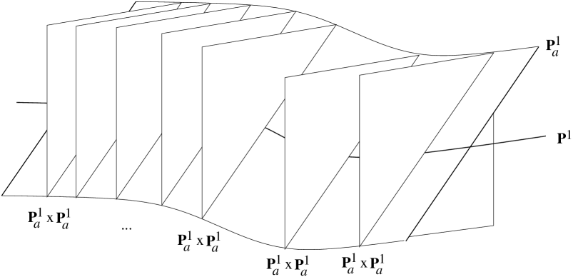
Figure 5: The moduli space $\mathcal{M}(\sigma_{*}l-\sigma_{*}E_{1})$.

Since in our example all the curves are topologically spheres, there are generically no vector fields in the low-energy theory. However, at the points where there is a transition between the two-fivebrane branch and the single fivebrane branch, additional low-energy fields can appear. These correspond to membranes which stretch between the two fivebranes becoming massless as the fivebranes intersect.

5.2 $[W]=\sigma_{*}l-\sigma_{*}E_{1}+F$

We can generalize the previous example by including a fiber component in the class of $W$, so that

$$[W]=\sigma_{*}l-\sigma_{*}E_{1}+F$$ (5.29)

Note that from (3.6) this class is effective.

We immediately see that one simple possibility is that $W$ splits into two curves

$$W=W_{0}+W_{F}$$ (5.30)

where

$$[W_{0}]=\sigma_{*}l-\sigma_{*}E_{1},\qquad[W_{F}]=F$$ (5.31)

The moduli space of the $W_{0}$ component will be exactly the same as our previous example, while for the pure fiber component, as given in equation (4.3), the moduli space is locally $B\times\mathbf{P}^{1}_{a}$. Since the base in this example is $dP_{8}$ here we conclude that, when the curve splits, this part of the moduli space is just the product of the moduli spaces for $W_{0}$ and $W_{F}$, that is

$$\mathcal{M}(\sigma_{*}l-\sigma_{*}E_{1})\times\left(dP_{8}\times\mathbf{P}^{1}_{a}\right)$$ (5.32)

where $\mathcal{M}(\sigma_{*}l-\sigma_{*}E_{1})$ was given above in (5.28). Physically we have two fivebranes, one wrapped on the fiber and one on the base, which can each move independently. As discussed above, for the curve wrapped on the base there are certain special points in moduli space where it splits into a pair of fivebranes, so that, at these special points, we have a total of three independent fivebranes. Since the curves of the base are all topologically spheres, their genus is zero. Hence, the only vector multiplets come from the fivebrane wrapping the fiber which, being topologically a torus with $g=1$, gives a $U(1)$ theory. Generically, the five brane wrapping the fiber $W_{F}$ does not intersect the fivebranes in the base $W_{0}$. However, there is a curve of points in the moduli space of $W_{F}$ where both fivebranes are in the same position in $S^{1}/Z_{2}$, with the same value of $a$, and $W_{0}$ lies above $W_{B}$ in the Calabi–Yau fibration. Generically, this gives a single intersection. However, there is a special point, when the base curves splits, as in (5.20) and (5.21), and the fiber component intersects exactly the point where the two base curves intersect. At such a point in moduli space, we have three fivebranes intersecting at a single point in the Calabi–Yau threefold. These different possible intersections are shown in Figure 6. Generically, we expect there to be additional multiplets in the low-energy theory at such points.

Figure 6: Possible enhancements in the moduli space of $[W]=\sigma_{*}l-\sigma_{*}E_{1}+F$. The first figure is where the curve in the base $W_{0}$ does not split. The second gives two possible cases when $W_{0}$ splits.

We might expect that there is also a component of the moduli space where the curve $W$ does not split at all, that is, where we have a single fivebrane in the class $\sigma_{*}l-\sigma_{*}E_{1}+F$. To analyze this second possibility we simply follow the analysis given above, where we first consider the moduli space of the image $C$ of $W$ in the base and then find the moduli space of curves which project down to the same given curve $C$.

Since the projection of $F$ onto the base is zero, the image of $[W]$ in the base is $\Omega=l-E_{1}$, as above. Thus many of the results of the previous discussion carry over to this situation. The moduli space of $C$ is given by (5.8). At a generic point in moduli space $S_{C}=\pi^{-1}(C)$ is a K3 surface, while at the seven special points where $C$ splits, the surface above each of the two components of $C$ is a $dP_{9}$ surface. If we consider first a generic point in the moduli space, $W$ is again a section of the K3 surface, but must now be in the class $\sigma_{*}l-\sigma_{*}E_{1}+F$. How many such sections are there? It turns out that for generic K3 there are none. We can see this as follows. By adjunction, since the genus of $C$ was zero, we showed in equation (5.17) that its class in $S_{C}$ satisfies $D_{C}\cdot D_{C}=-2$. The identical calculation applies to any section, since all sections have genus zero. Thus, in particular, we have

$$[W]_{C}\cdot[W]_{C}=-2$$ (5.33)

where by $[W]_{C}$, we mean the class of $W$ in $S_{C}$. However, from the map between classes (5.13), it is clear that $[W]_{C}=D_{C}+F_{C}$. Since $D_{C}$ is the class of the zero section, we have $D_{C}\cdot F_{C}=1$. For the fiber class we always have $F_{C}\cdot F_{C}=0$. Hence, we must also have

$$[W]_{C}\cdot[W]_{C}=0$$ (5.34)

This contradiction implies that there can be no sections of $S_{C}$ in the class $\sigma_{*}l-\sigma_{*}E_{1}+F$. In other words, we have shown that, generically, we cannot have just a single fivebrane in the class $\sigma_{*}l-\sigma_{*}E_{1}+F$. Rather, the fivebrane always splits into a pure fiber component and a pure base component, as described above.

What about the special points in the moduli space where the curve $C$ splits into two? Do we still have to have a separate pure fiber component? The answer is no, for the reason that, as discussed above, the space above each component is a $dP_{9}$ surface and, unlike the K3 case, there are many more algebraic classes on $dP_{9}$ than just the zero section and the fiber. Specifically, suppose there is no separate pure fiber component in $W$ and consider the point where $C$ splits into $C_{1}+C_{2}$ with $[C_{1}]=l-E_{1}-E_{2}$ and $[C_{2}]=E_{2}$. The actual curve $W$ must also split into $W_{1}$ and $W_{2}$. Given that each component must be effective, we then have two possibilities, depending on which component includes the fiber class

$$\begin{gathered}{}[W_{1}]=\sigma_{*}l-\sigma_{*}E_{1}-\sigma_{*}E_{2}+F,\qquad[W_{2}]=\sigma_{*}E_{2}\\ \text{or}\\ {}[W_{1}]=\sigma_{*}l-\sigma_{*}E_{1}-\sigma_{*}E_{2},\qquad[W_{2}]=\sigma_{*}E_{2}+F\end{gathered}$$ (5.35)

Let us concentrate on the first case, although a completely analogous analysis holds in the second example. Above, we calculated the number of curves in the case where the class contains no $F$. We found, for instance, that if $[W_{2}]=\sigma_{*}E_{2}$ then $W_{2}$ is required to be precisely the section $C_{2}$ and there is no moduli space for moving the curve in the fiber direction. The situation is richer, however, for the class with an $F$ component. We will discuss this is more detail in section 6.3 below, but it turns out that there are 240 different sections of $dP_{9}$ in the class $[W_{1}]=\sigma_{*}l-\sigma_{*}E_{1}-\sigma_{*}E_{2}+F$. It is a general result, just repeating the calculation that led to (5.26), that any section of the $dP_{9}$ has self-intersection $-1$. Consequently none of the 240 different sections in the class $\sigma_{*}l-\sigma_{*}E_{1}-\sigma_{*}E_{2}+F$ can be deformed in the fiber direction and, hence, they simply provide a discrete set of different $W_{1}$ which all map to the same $C_{1}$. Furthermore, one can show that none of these sections intersect the base of the Calabi–Yau manifold. Thus, since, in the case we are considering, $W_{2}$ lies solely in the base, we find that $W_{1}$ and $W_{2}$ can never overlap. Their relative positions within the Calabi–Yau threefold are shown in Figure 7.

Figure 7: $W=W_{1}+W_{2}$ in the case where $[W_{1}]=\sigma_{*}l-\sigma_{*}E_{1}-\sigma_{*}E_{2}+F$ and $[W_{2}]=\sigma_{*}E_{2}$.

It is important to note that these curves are completely stuck within the Calabi–Yau threefold. They cannot combine into a single curve and move away from the exceptional point in the moduli space of $C$ (the projection of $W$ into the $dP_{8}$ base) where $C$ splits into two curves. Furthermore, we have argued that they cannot move in the fiber. Thus, the only moduli for this component of the moduli space are the positions of the two fivebranes in the orbifold interval and the values of their axions, giving a moduli space of

$$\mathbf{P}^{1}_{a}\times\mathbf{P}^{1}_{a}$$ (5.36)

Furthermore, since all the sections of $dP_{9}$ are topologically spheres, there are no vector multiplets in this part of the moduli space. As we noted above, the fivebranes cannot overlap. Hence, there is no possibility of additional multiplets appearing. Finally, we note that there were seven ways $C$ could split into $C_{1}+C_{2}$, and, for each splitting, $W$ can decompose one of two ways (5.35). Since for each decomposition there are 240 distinct sections, we see that there is a grand total of 3360 ways of making the analogous decomposition to that we have just discussed.

In conclusion, we see that the full moduli space for $[W]=\sigma_{*}l-\sigma_{*}E_{1}+F$ has a relatively rich structure. It splits into a large number of disconnected components. The largest component is where $W$ splits into separate fiber and base components, $W=W_{0}+W_{F}$. The moduli space is then given by (5.32), which includes the possibility of the base component splitting. There are then 3360 disconnected components where $W$ splits into two irreducible components, one of which includes the fiber class $F$. We can summarize this structure in a table

$$\begin{array}[]{c|cc}[W]&\text{genus}&\text{moduli space}\\ \hline\cr\hline\cr(\sigma_{*}l-\sigma_{*}E_{1})+(F)&0+1&\left(\left[\mathbf{P}^{1}-7\text{ pts.}\right]\times\mathbf{P}^{1}_{a}\right)\times\left(dP_{8}\times\mathbf{P}^{1}_{a}\right)\\ (\sigma_{*}l-\sigma_{*}E_{1}-\sigma_{*}E_{2})+(\sigma_{*}E_{2})+(F)&0+0+1&\mathbf{P}^{1}_{a}\times\mathbf{P}^{1}_{a}\times\left(dP_{8}\times\mathbf{P}^{1}_{a}\right)\\ \hline\cr(\sigma_{*}l-\sigma_{*}E_{1}-\sigma_{*}E_{2}+F)+(\sigma_{*}E_{2})&0+0&\mathbf{P}^{1}_{a}\times\mathbf{P}^{1}_{a}\end{array}$$ (5.37)

Here, the first column gives the homology classes in $X$ of the different components of $W$. The first two rows describe the moduli space (5.32) where $W$ splits into $W_{0}+W_{F}$, first for a generic component in the base and then at one of seven points where the base component splits. The final row describes one of the 3360 disconnected components of the moduli space (5.36). From the genus count, we see that in the first two cases we expect a $U(1)$ gauge field on the fivebrane which wraps the fiber, while in the last case there are no vector multiplets. As we have noted, the component of the moduli given in the first two rows has the possibility that the fivebranes intersect leading to additional low-energy fields, as depicted in Figure 6. The disconnected components, have no such enhancement mechanism. Furthermore, their moduli space is severely restricted since neither fivebrane can move within the Calabi–Yau manifold.

6 General procedure for analysis of the moduli space

From the examples above, we can distill a general procedure for the analysis of the generic moduli space. We start with a general fivebrane curve in the class

$$[W]=\sigma_{*}\Omega+fF$$ (6.1)

Furthermore, $[W]$ is assumed to be effective, so that, by (3.6), $\Omega$ is some effective class in $H_{2}(B,\mathbf{Z})$ and $f\geq 0$. We need to first find the moduli space of the projection $C$ of $W$ onto the base. One then finds all the curves in the full Calabi–Yau threefold in the correct homology class which project onto $C$. In general, we will find that the above case, where the space $S_{C}=\pi^{-1}(C)$ above $C$ was a K3 surface, is the typical example. There, we found that no irreducible curve which projects onto $C$ could include a fiber component in its homology class. Hence, $[W]$ splits into a pure base and a pure fiber component. One exception, as we saw above, is when $S_{C}$ is a $dP_{9}$ surface. In the following, we will start by analysing the generic case and then give a separate discussion for the case where $dP_{9}$ appears.

6.1 Decomposition of the moduli space

Any curve $W$ in the Calabi–Yau threefold can be projected to the base using the map $\pi$. In general, $W$ may have one or many components. Typically, a component will project to a curve in the base. However, there may also be components which are simply curves wrapping the fiber at different points in the base. These curves will all project to points in the base rather than curves. Thus, the first step in analyzing the moduli space is to separate out all such curves. We therefore write $W$ as the sum of two components, each of which may be reducible,

$$W=W_{0}+W_{F}$$ (6.2)

but with the assumption that none of the components of $W_{0}$ are pure fiber components. For general $[W]$ given in (6.1), the classes of these components are

$$[W_{0}]=\sigma_{*}\Omega+nF\qquad[W_{F}]=(f-n)F$$ (6.3)

with $0\leq n\leq f$, since each class must be separately effective. Note that, although $W_{0}$ has no components which are pure fiber, its class may still involve $F$ since, in general, components of $W_{0}$ can wrap around the fiber as they wrap around a curve in the base. Except when $n=f$, so $W_{F}=0$, $W$ has at least two components in this decomposition and so there are at least two five-branes.

In general, the decomposition (6.2) splits the moduli space into $f+1$ different components depending on how we partition the $f$ fiber classes between $[W_{0}]$ and $[W_{F}]$. Within a particular component, the moduli space is a product of the moduli space of $W_{0}$ and $W_{F}$. If $\mathcal{M}_{F}((f-n)F)$ is the moduli space of $W_{F}$ and $\mathcal{M}_{0}(\sigma_{*}\Omega+nF)$ is the moduli space of $W_{0}$, we can then write the full moduli space as

$$\mathcal{M}(\sigma_{*}\Omega+fF)=\bigcup_{n=0}^{f}\mathcal{M}_{0}(\sigma_{*}\Omega+nF)\times\mathcal{M}((f-n)F)$$ (6.4)

The problem is then reduced to finding the form of the moduli spaces for $W_{0}$ and $W_{F}$. The latter moduli space has already been analyzed in section 4.2. We found that, locally,

$$\mathcal{M}((f-n)F)=\left(B\times\mathbf{P}^{1}_{a}\right)^{f-n}/\mathbf{Z}_{f-n}$$ (6.5)

Thus we are left with $\mathcal{M}_{0}(\sigma_{*}\Omega+nF)$, which can be analyzed by the projection techniques we used in the preceding examples.

Projecting $W_{0}$ onto the base, we get a curve $C$ in the class $\Omega$ in $B$. Let us call the moduli space of such curves in the base $\mathcal{M}_{B}(\Omega)$. This space is relatively easy to analyze since we know the form of $B$ explicitly. In general, it can be quite complicated with different components and branches as curves degenerate and split. To find the full moduli space $\mathcal{M}_{0}(\sigma_{*}\Omega+nF)$, we fix a point in $\mathcal{M}_{B}(\Omega)$ giving a particular curve $C$ in $B$ which is the projection of the original curve $W_{0}$ in the Calabi–Yau threefold. In the following, we will assume that $C$ is not singular. By this we mean that it does not, for instance, cross itself or have a cusp in $B$. If it is singular, it is harder to analyze the space of curves $W_{0}$ which project onto $C$. In general, $C$ splits into $k$ components, so that

$$C=C_{1}+\dots+C_{k}$$ (6.6)

We then also have

$$\Omega=\Omega_{1}+\dots+\Omega_{k}$$ (6.7)

where $\Omega_{i}=[C_{i}]$ and, so, must be an effective class on the base for each $i$. Clearly if the curve in the base has more than one component then so does the original curve $W_{0}$, so that

$$W_{0}=W_{1}+\dots+W_{k}$$ (6.8)

with $\pi(W_{i})=C_{i}$. In general, the class of $W_{0}$ will be partitioned into a sum of classes of the form

$$[W_{i}]=\sigma_{*}\Omega_{i}+n_{i}F$$ (6.9)

where, for each curve to be effective, $n_{i}\geq 0$ and $n_{1}+\dots+n_{k}=n$, leading to a number of different possible partitions.

One now considers a particular component $C_{i}$. To find the moduli space over $C_{i}$, one needs to find all the curves $W_{i}$ in $X$ in the cohomology class $\sigma_{*}\Omega_{i}+n_{i}F$ which project on $C_{i}$. Recall, in addition, that we have assumed in our original partition (6.2) that $[W_{i}]$ contains no pure fiber components. Repeating this procedure for each component and for each partition of the $n$ fibers into $\{n_{i}\}$, gives the moduli space over a given point $C$ in $\mathcal{M}_{B}(\Omega)$ and, hence, the full moduli space.

Consequently, we have reduced the problem of finding the full moduli space $\mathcal{M}_{0}(\sigma_{*}\Omega+nF)$ to the following question. To simplify notation, let $R$ be the given irreducible curve $C_{i}$ in the base, and let $V$ be the corresponding curve $W_{i}$ in the full Calabi–Yau threefold. Let us further write the class $\Omega_{i}$ of $C_{i}$ as $\Lambda$ and write $m$ for $n_{i}$. Our general problem is then to find, for the given irreducible curve $R$ in the effective homology class $\Lambda$, what are all the curves $V$ in the Calabi–Yau threefold in the class $\sigma_{*}\Lambda+mF$, where $m\geq 0$ which project onto $R$. Necessarily, all the curves $V$ which project into $R$ lie in the surface $S_{R}=\pi^{-1}(R)$. By construction, $S_{R}$ is elliptically fibered over the base curve $R$. Furthermore, typically, the map from $V$ to $R$ wraps $R$ only once. It is possible that $R$ is some number $q$ of completely overlapping curves in $B$, so that $[R]=q\Gamma$ for some effective class $\Gamma$ in $B$. Then the map from $V$ to $R$ wraps the base curve $q$ times. This will occur in one of the examples we give later in the paper, but here, since we are discussing generic properties, let us ignore this possibility. Then, assuming $R$ is not singular, the map is invertible and we see that $V$ must be a section of the fibered surface $S_{R}$.

Furthermore, we note that $S_{R}$ can be characterized by the genus $g$ of the base curve $R$ and the number of singular fibers. The former is, by adjunction, given by

$$2g-2=\left(K_{B}+\Lambda\right)\cdot\Lambda$$ (6.10)

The latter is also a function only of the class $\Lambda$ of $R$ and can be found by intersecting the discriminant class $[\Delta]$ with $\Lambda$. Since $[\Delta]=-12K_{B}$, the number of singular fibers must be of the form $12p$ with

$$p=-K_{B}\cdot\Lambda$$ (6.11)

where $p$ is an integer. If $p$ is negative, the curve $R$ lies completely within the discriminant curve of the elliptically fibered Calabi–Yau manifold. This means that every fiber above $R$ is singular. The form of $S_{R}$ then depends on the structure of the particular fibration of the Calabi–Yau threefold. Since we want to consider generic properties of the moduli space, we will ignore this possibility and restrict ourselves to the case where $p$ is non-negative. We note that this is not very restrictive. For del Pezzo and Enriques surfaces $-K_{B}$ is nef, meaning that its intersection with any effective class in the base is non-negative. Hence, since $\Lambda$ must be effective, we necessarily have $p\geq 0$. The only exceptions, are Hirzebruch surfaces $F_{r}$ with $r\geq 3$ and where $\Lambda$ includes the negative section $\mathcal{S}$.

Finally, then, finding the full moduli space $\mathcal{M}_{0}(\sigma_{*}\Omega+nF)$ has been reduced to the following problem

• For a given irreducible curve $R$ in the base $B$ with homology class $\Lambda$, find the moduli space of sections $V$ of the surface $S_{R}=\pi^{-1}(R)$ in the homology class $\sigma_{*}\Lambda+mF$ in the full Calabi–Yau threefold $X$, where $m\geq 0$.

  $S_{R}$ is characterized by $g=\text{genus}\,(C)$, as given in (6.10), and $p$, where $12p$ is the number of singular elliptic fibers, as given in (6.11). Consequently, we write this moduli space as $\mathcal{M}(g,p;m)$.

We will assume that $p\geq 0$. This is necessarily true, except when $B$ is an $F_{r}$ surface with $r\geq 3$ and $\Lambda$ contains the class of the section at infinity $\mathcal{S}$.

6.2 The generic form of $\mathcal{M}(g,p;m)$

To understand the sections of $S_{R}$, we start by finding the algebraic classes on $S_{R}$. As for the K3 surface, a generic surface $S$ has no algebraic classes since $h^{2,0}\neq 0$. For $S_{R}$, we know that two classes are necessarily present, the class of the zero section $D_{R}$ and the fiber class $F_{R}$. However, generically, there need not be any other classes. Additional classes may appear for special choices of complex structure, but here we will consider only the generic case. The obvious exception is the case where $g=0$ and $p=1$. From equations (6.10) and (6.11), this implies that $R$ is an exceptional curve in $B$. The surface $S_{R}$ is then an elliptic fibration over $\mathbf{P}^{1}$ with 12 singular fibers, which is a $dP_{9}$ surface. In this case $h^{2,0}=0$ and every class in $H_{2}(S_{R},\mathbf{Z})$ is algebraic. We will return to this case in the next section. The inclusion map $i_{R}:S_{R}\to X$, gives a natural map between classes in $S_{R}$ and in $X$

$$i_{R*}:H_{2}(S_{R},\mathbf{Z})\to H_{2}(X,\mathbf{Z})$$ (6.12)

In general, with only two classes the map is simple. By construction, we have

$$i_{R*}D_{R} =\sigma_{*}\Lambda$$ (6.13)

$$i_{R*}F_{R} =F$$

Just as in the K3 example, we will find that the existence of only two classes strongly constrains the moduli space $\mathcal{M}(g,p;m)$. We can find the analog of the contradiction of equations (5.33) and (5.34) as follows. Let $K_{S_{R}}$ be the cohomology class of the canonical bundle of the surface. Since both $V$ and $R$ are sections, they have the same genus $g$. By the Riemann–Hurwitz formula and adjunction, we have

$$2g-2=\left(K_{S_{R}}+D_{R}\right)\cdot D_{R}=K_{S_{R}}\cdot D_{R}+D_{R}\cdot D_{R}$$ (6.14)

where $D_{R}$ is the class of the zero section, and

$$2g-2=\left(K_{S_{R}}+[V]_{R}\right)\cdot[V]_{R}=K_{S_{R}}\cdot[V]_{R}+[V]_{R}\cdot[V]_{R}$$ (6.15)

where $[V]_{R}$ the class of $V$ in $S_{R}$. We also have, for the fiber, by a similar calculation, since it has genus one and, since two generic fibers do not intersect, $F_{R}\cdot F_{R}=0$, that

$$0=\left(K_{S_{R}}+F_{R}\right)\cdot F_{R}=K_{S_{R}}\cdot F_{R}$$ (6.16)

Finally, since we require in $X$ that $[V]=\sigma_{*}\Lambda+mF$ and since we assume that no additional classes exist on $S_{R}$,

$$[V]_{R}=D_{R}+mF_{R}$$ (6.17)

Substituting this expression into (6.15) and using (6.14), we find

$$[V]_{R}\cdot[V]_{R}=D_{R}\cdot D_{R}$$ (6.18)

On the other hand, given that $F_{R}\cdot D_{R}=1$ because the fiber intersects a section at one point, we can compute the self-intersection of $[V]_{R}=D_{R}+mF_{R}$, explicitly, yielding

$$[V]_{R}\cdot[V]_{R}=D_{R}\cdot D_{R}+2m$$ (6.19)

Comparing (6.18) with (6.19), we are left with the important conclusion that we must have $m=0$. This implies that, generically, no component of $W_{0}$ can contain any fibers in its homology class. We conclude that

$$\mathcal{M}(g,p;m)=\emptyset\qquad\text{unless}\quad m=0$$ (6.20)

In fact, we can go further. Since we require $m=0$, we see from (6.17) that $V$ is in the same class $D_{R}$ as the zero section $R$. Using the Riemann–Roch formula and Kodaira’s description of elliptically fibered surfaces, one can show that the canonical class in the cohomology of $S_{R}$ is given by

$$K_{S_{R}}=\left(2g-2+p\right)F_{R}$$ (6.21)

Then, substituting this expression into (6.14), we see that

$$D_{R}\cdot D_{R}=-p$$ (6.22)

Thus we see that for $p>0$, $R$ is an exceptional divisor and cannot be deformed in $S_{R}$. Consequently, all the fivebrane can do is to move in the orbifold direction and change its value of $a$, so we have a moduli space of $\mathbf{P}^{1}_{a}$. If $p=0$, the fibration is locally trivial. It may or may not be globally trivial. However, it is always globally trivial when pulled back to some finite cover of the base. Every section is in the class $D_{R}$ and the moduli space simply corresponds to moving the fivebrane in the fiber direction and in $S^{1}/Z_{2}$ and $a$. If the original fibration was globally trivial, this yields a moduli space of $E\times\mathbf{P}^{1}_{a}$, where $E$ is an elliptic curve describing motion of $V$ in the fiber direction. If it was only locally trivial, then these deformations in the fiber directions still make sense over the cover, but only a finite subset of them happens to descend, so the actual moduli space consists in this case of some finite number of copies of $\mathbf{P}^{1}_{a}$.

In summary, we see that, generically, if we exclude the case $g=0$, $p=1$ where $S_{R}$ is a $dP_{9}$ surface,

$$\mathcal{M}(g,p;m)=\emptyset\qquad\text{for}\quad m>0$$ (6.23)

while if $m=0$ we have,

$$\mathcal{M}(g,p;0)=\begin{cases}N\mathbf{P}^{1}_{a}&\text{if }p=0\text{ and the fibration is not globally trivial}\\ E\times\mathbf{P}^{1}_{a}&\text{if }p=0\text{ and the fibration is globally trivial}\\ \mathbf{P}^{1}_{a}&\text{if }p>0\end{cases}$$ (6.24)

where $N$ is some integer depending on the global structure of $S_{C}$. In each case, the gauge group on the fivebrane is given by $U(1)^{g}$ where $g$ is the genus of the curve $R$ in the base $B$. Since both $R$ and $V$ are sections of $S_{R}$, this is equal to the genus of the curve $V$ in the space $X$.

6.3 The $dP_{9}$ exception and ${\cal{M}}(0,1;m)$

As we have mentioned, the obvious exception to the above analysis is when $S_{R}$ is a $dP_{9}$ surface. This occurs when the base curve $R$ is topologically $\mathbf{P}^{1}$ and there are 12 singular elliptic fibers in $S_{R}$, that is if $[R]=\Lambda$ in the base $B$,

$$2g-2=\left(K_{B}+\Lambda\right)\cdot\Lambda=-2,\qquad p=-K_{B}\cdot\Lambda=1$$ (6.25)

As we mentioned above, this implies that $R$ is an exceptional curve in the base. In this case, $D_{R}$ and $F_{R}$ are not the only generic algebraic classes on $S_{R}$. Rather, since $h^{2,0}=0$, every integer class in $dP_{9}$ is algebraic. The surface $dP_{9}$ can be described as the plane $\mathbf{P}^{2}$ blown up at nine points which are at the intersection of two cubic curves. Consequently, there are ten independent algebraic classes on $dP_{9}$, the image $l^{\prime}$ of the class of a line in $\mathbf{P}^{2}$ and the nine exceptional divisors, $E^{\prime}_{i}$ for $i=1,\dots,9$, corresponding to the blown up points. Here we use primes to distinguish these classes from classes in the base $B$ of the Calabi–Yau threefold (specifically, the $E_{i}$ classes in $B$ when the base is a del Pezzo surface).

The point here is that, in the full Calabi–Yau manifold $X$, there are only two independent classes associated with $S_{R}$, namely, the class of the base curve $\sigma_{*}\Lambda$ and the fiber class $F$. Consequently, if $i_{R}:S_{R}\to X$ is the inclusion map from the $dP_{9}$ surface into the Calabi–Yau threefold, the corresponding map between classes

$$i_{R*}:H_{2}(S_{R},\mathbf{Z})\to H_{2}(X,\mathbf{Z})$$ (6.26)

must have a non-empty kernel, since it maps the ten independent classes on $S_{R}$ mentioned above into only two in $X$. Recall that our goal is to find the set of sections $V$ of $S_{R}$ which are in the class $\sigma_{*}\Lambda+mF$ in $X$. Previously, we found that generically there were no such sections unless $m=0$. This followed from equations (6.14) to (6.19). Now, the appearance of a kernel in the map (6.26), means that $[V]_{R}$ is no longer necessarily of the form $D_{R}+mF_{R}$, as in equation (6.17). Consequently we can no longer conclude that we must have $m=0$. In fact, as we will see, there are several different sections $V$ in the same class $\sigma_{*}\Lambda+mF$ in $X$ with $m>0$.

Let us start by recalling why a $dP_{9}$ surface is also an elliptic fibration. Viewed as $\mathbf{P}^{2}$ blown up at nine points, we have the constraint that the nine points lie at the intersection of two cubics. This is represented in Figure 8. The cubics can be written as two third-order homogeneous polynomials in homogeneous coordinates $[x,y,z]$ on $\mathbf{P}^{2}$. Let us call these polynomials $f$ and $g$. Clearly any linear combination $af+bg$ defines a new cubic polynomial. By construction, this polynomial also passes through the same nine points. Since the overall scale does not change the cubic, the set of cubics is given by specifying $a$ and $b$ up to overall scaling. Thus, we have a $\mathbf{P}^{1}$ of cubics passing through the nine points. Since each cubic defines an elliptic curve, we can think of this as an elliptic fibration over $\mathbf{P}^{1}$. Furthermore, the cubics cannot intersect anywhere else in $\mathbf{P}^{2}$. The space of cubics spans the whole of the plane and, further, it blows up each intersection point into a $\mathbf{P}^{1}$ of distinct points, one point in $\mathbf{P}^{1}$ for each cubic passing through the intersection. Thus the space of cubics is giving an alternative description of the $dP_{9}$ surface. In addition, we note that each of the exceptional divisors $E^{\prime}_{i}$, the blow-ups of the intersection points, is a $\mathbf{P}^{1}$ surface which intersects each fiber at a single point, and so corresponds to section of the fibration. Furthermore, the anti-canonical class of $dP_{9}$ is given by

$$-K_{S_{R}}=3l^{\prime}-E^{\prime}_{1}-\dots-E^{\prime}_{9}=F_{R}$$ (6.27)

and is precisely the class of the cubics passing through the nine intersection points. It follows that

$$K_{S_{R}}=-F_{R}$$ (6.28)

which, since $g=0$ and $p=1$, agrees with the general expression (6.21).

Figure 8: The space $dP_{9}$

It is natural to ask if there are other sections of $dP_{9}$ aside from the exceptional curves $E^{\prime}_{i}$. We first note that any section of $dP_{9}$ is exceptional, with $[V]_{R}\cdot[V]_{R}=-1$. This follows from (6.15) and (6.27), recalling that any section will have genus zero and intersects the fiber (the anti-canonical class) only once. Next, we recall that there is a notion of addition of points on elliptic curves. Consequently, we can add sections point-wise to get a new section. Thus, we see that the set of sections forms an infinite Abelian group containing all the exceptional curves on the $dP_{9}$ surface. From the point of view of curves in $\mathbf{P}^{2}$, these additional exceptional classes correspond to curves of higher degree passing through the nine intersection points with some multiplicity (see for instance [7]). In general, we can write an exceptional class (except the classes $E^{\prime}_{i}$) as

$$Q=ql^{\prime}-\sum q_{i}E^{\prime}_{i}$$ (6.29)

such that

$$q,q_{i}\geq 0,\quad q^{2}-\sum q_{i}^{2}=-1,\quad 3q-\sum q_{i}=1$$ (6.30)

where the first condition is required in order to describe an effective curve in $\mathbf{P}^{2}$, the second condition gives $Q\cdot Q=-1$ and the third condition gives $Q\cdot F_{R}=1$. The appearance of an infinite number of exceptional classes means that these equations have an infinite number of solutions for $i=1,\dots,9$.

Having identified all the relevant classes in $dP_{9}$, we can now turn to a description of the map (6.26). First, we note that the group structure of the set of sections means that we can choose any section as part of the basis of classes. In our case, we have singled out one section as the class of the base curve $R$. Thus, without loss of generality, we can identify this class with one of the $E^{\prime}_{i}$, for example, $E^{\prime}_{9}$. Thus we set

$$D_{R}=E^{\prime}_{9}$$ (6.31)

By construction, we know that $D_{R}$ maps to $\sigma_{*}\Lambda$ and $F_{R}$ maps to $F$ under $i_{R*}$. Thus, in terms of $l^{\prime}$ and $E^{\prime}_{i}$, we have, using (6.27) and the generic result (6.13),

$$\begin{gathered}i_{R*}E^{\prime}_{9}=\sigma_{*}\Lambda\\ i_{R*}\left(3l^{\prime}-E^{\prime}_{1}-\dots-E^{\prime}_{9}\right)=F\end{gathered}$$ (6.32)

We now need to understand how the remaining independent classes $E^{\prime}_{1},\dots,E^{\prime}_{8}$ map under $i_{R*}$. We first note that, since all these classes are sections, they must project onto the class $\Lambda$ in the base. The only ambiguity is how many multiples of the fiber class $F$ each contains. Thus, we know

$$i_{R*}E^{\prime}_{i}=\sigma_{*}\Lambda+c_{i}F$$ (6.33)

for some $c_{i}$. The easiest way to calculate $c_{i}$ is to recall that a class in $H_{2}(X,\mathbf{Z})$ is uniquely determined by its intersection numbers with a basis of classes in $H_{4}(X,\mathbf{Z})$. A suitable basis was given in section 3.2. In particular, we can consider the intersection of $E^{\prime}_{i}$ with the class $D$ of base $B$ of the full Calabi–Yau threefold. We note that $E^{\prime}_{i}\cdot E^{\prime}_{9}=0$ for $i=1,\dots,8$, so the extra sections $E^{\prime}_{i}$ do not intersect the base $R$ of the $dP_{9}$. However, since $R$ describes the intersection of $B$ with the $dP_{9}$ surface $S_{R}$, we see that the extra classes cannot intersect $B$. Thus, we must have

$$i_{R*}E^{\prime}_{i}\cdot D=0\qquad\text{for}\quad i=1,\dots,8$$ (6.34)

From the table of intersections (3.4), using (6.25), we see that we must have $c_{i}=1$ for $i=1,\dots,8$. Together with the result (6.32) we find, in conclusion, that the map (6.26) is given by

$$i_{R*}l^{\prime} =3\sigma_{*}\Lambda+3F$$ (6.35)

$$i_{R*}E^{\prime}_{i} =\sigma_{*}\Lambda+F\qquad\text{for}\quad i=1,\dots,8$$

$$i_{R*}E^{\prime}_{9} =\sigma_{*}\Lambda$$

demonstrating explicitly that the map has a kernel.

Having identified the map, we would now like to return to our original question, which was how many sections are there in the class $\sigma_{*}\Lambda+mF$ and what is their moduli space. The second part is easy to answer. We have noted that all sections are exceptional with self-intersection $-1$. This implies that they cannot be moved within the $dP_{9}$ surface. However, they can move in the orbifold and have different values of the axion. Consequently, each section has a moduli space of $\mathbf{P}^{1}_{a}$. If there are a total of $N(m)$ sections for a given $m$, then the total moduli space $\mathcal{M}(0,1;m)$ has the form

$$\mathcal{M}(0,1;m)=N(m)\mathbf{P}^{1}_{a}$$ (6.36)

The value of $N(m)$ is a problem in discrete mathematics. Recall that the class of a general section had the form given in (6.29). Under the map $i_{R*}$ this maps into

$$i_{R*}Q=\sigma_{*}\Lambda+\left(q_{9}+1\right)F$$ (6.37)

where we have used the condition $3q-\sum q_{i}=1$. Thus, we can summarize the problem as finding the number of solutions to

$$q^{2}-\sum q_{i}^{2}+1 =0$$ (6.38)

$$3q-\sum q_{i} =1$$

with

$$q\geq 0,\quad q_{i}\geq 0,\quad q_{9}=m-1$$ (6.39)

We will not solve this problem in general, but just note the solution of $m=0$ and $m=1$. The former case is not actually included in the above form, since it implies $q_{9}=-1$. However, this case is easy to analyze since, with $m=0$, we see, from (3.4) and (6.25), that the intersection of $[V]=\sigma_{*}\Lambda$ with the base class $D$ of the Calabi–Yau manifold is $-1$. Consequently, a component of $V$ must lie in the base $B$. Since, by assumption, $V$ is irreducible, this means that the whole of $V$ lies in $B$. Thus, $V$ can only be the base section $R$ in the $dP_{9}$ surface. Thus we conclude that, for a $dP_{9}$ surface $S_{R}$, $N(0)=1$. That is,

$$\mathcal{M}(0,1;0)=\mathbf{P}^{1}_{a}$$ (6.40)

corresponding to moving the single curve $R$ in $S^{1}/Z_{2}$. This result was used in analyzing the example in section 5.1.

For $m=1$, there are 240 solutions to the equations (6.38), that is $N(1)=240$. The easiest way to see this is to note that $m=1$ implies $q_{9}=0$. Thus, we can ignore $E^{\prime}_{9}$. Effectively, one is then trying to count the number of exceptional curves on a $dP_{8}$ surface. This is known to be a finite number, $240$ [31]. Explicitly, they are of the following forms

$$E^{\prime}_{i}$$ (6.41)

$$l^{\prime}-E^{\prime}_{i}-E^{\prime}_{j}$$

$$2l^{\prime}-E^{\prime}_{i_{1}}-\dots-E^{\prime}_{i_{5}}$$

$$3l^{\prime}-2E^{\prime}_{i}-E^{\prime}_{i_{1}}-\dots-E^{\prime}_{i_{6}}$$

$$4l^{\prime}-2E^{\prime}_{i_{1}}-\dots-2E^{\prime}_{i_{3}}-E^{\prime}_{i_{4}}-\dots-E^{\prime}_{i_{8}}$$

$$5l^{\prime}-2E^{\prime}_{i_{1}}-\dots-2E^{\prime}_{i_{6}}-E^{\prime}_{i_{7}}-E^{\prime}_{i_{8}}$$

$$6l^{\prime}-2E^{\prime}_{i_{1}}-\dots-2E^{\prime}_{i_{7}}-3E^{\prime}_{i_{8}}$$

where all the indices run from $1$ to $8$. One can see, using (6.35), that all these classes map under $i_{R*}$ to $\sigma_{*}\Lambda+F$. Again, since none of these sections can move in the $dP_{9}$ surface, the moduli space is simply 240 copies of $\mathbf{P}^{1}_{a}$,

$$\mathcal{M}(0,1;1)=240\,\mathbf{P}^{1}_{a}$$ (6.42)

This result was used in analyzing the example in section 5.2. We also note that none of these sections intersects the base section $R$.

7 A three-family $dP_{8}$ example

In the previous section we have given a general procedure for analyzing the moduli space of fivebranes wrapped on a holomorphic curve in a particular effective class in the Calabi–Yau manifold. The problem is of particular importance because it has been shown [15, 6, 7] that including fivebranes in supersymmetric M theory compactifications greatly enlarges the number of vacua with reasonable grand unified gauge groups and three families of matter.

In the remaining sections, we apply this procedure to some specific examples which arise in the construction of phenomenological models. We will find that the moduli spaces are very rich. Nonetheless, we will find that there are isolated parts of moduli space where the number of moduli is greatly reduced. We will not describe the full moduli spaces here, but rather consider various characteristic components.

Let us start with the example given in [6] and expanded upon in [7]. There, the base $B$ was a $dP_{8}$ surface and the class of the fivebranes was given by

$$[W]=2\sigma_{*}E_{1}+\sigma_{*}E_{2}+\sigma_{*}E_{3}+17F$$ (7.1)

where $l$ and $E_{i}$ for $i=1,\dots,8$ are the line class and the exceptional blow-up classes in the $dP_{8}$. Since $2E_{1}+E_{2}+E_{3}$ is effective in $dP_{8}$, this describes an effective class in the Calabi–Yau manifold. This choice of fivebrane class, together with a non-trivial $E_{8}$ bundle $V_{1}$, led to a low-energy $SU(5)$ theory with three families.

7.1 General decomposition

Let us follow exactly the procedure laid down in the previous section. First, we separate from $W$ all the pure fiber components, writing it as the sum of $W_{0}$ and $W_{F}$ as in (6.2). We write

$$[W_{0}]=2E_{1}+E_{2}+E_{3}+nF,\qquad[W_{F}]=(17-n)F$$ (7.2)

with $0\leq n\leq 17$. Unless $n=17$, we have at least two separate fivebranes. This splits the moduli space into several different components depending on the partition of 17 into $n$ and $17-n$, as given in (6.4). The moduli space for the pure fiber component $W_{F}$ is just the familiar form, read off from (6.5)

$$\mathcal{M}((17-n)F)=\left(dP_{8}\times\mathbf{P}^{1}_{a}\right)^{17-n}/\mathbf{Z}_{17-n}$$ (7.3)

More interesting is the analysis of the $W_{0}$ moduli space. As described above, the first step in the analysis is to project $W_{0}$ onto the base. This gives the curve $C$ which is in the homology class

$$[C]=2E_{1}+E_{2}+E_{3}$$ (7.4)

We then need to find the moduli space $\mathcal{M}_{B}(2E_{1}+E_{2}+E_{3})$ of $C$ in the base. We recall that the del Pezzo surface $dP_{8}$ can be viewed as $\mathbf{P}^{2}$ blown up at eight points. The exceptional classes $E_{i}$ each have a unique representative, namely the exceptional curve $\mathbf{P}^{1}$ at the $i$-th blown-up point. Furthermore, we have the intersection numbers $E_{i}\cdot E_{j}=-\delta_{ij}$. Thus $[C]$ has a negative intersection number with each of $E_{1}$, $E_{2}$ and $E_{3}$. This implies that it must have a component contained completely within each of the exceptional curves described by $E_{1}$, $E_{2}$ and $E_{3}$. Since these are all distinct, $C$ must be reducible into three components

$$C=C_{1}+C_{2}+C_{3}$$ (7.5)

where

$$[C_{1}]=2E_{1}\qquad[C_{2}]=E_{2}\qquad[C_{3}]=E_{3}$$ (7.6)

None of these components can be moved in the base, since they all have negative self-intersection number. Consequently, we have

$$\mathcal{M}_{B}(2E_{1}+E_{2}+E_{3})=\text{single pt.}$$ (7.7)

corresponding to three fivebranes, each wrapping a different exceptional curve.

Since the projection $C$ splits, so must the curve $W_{0}$ itself. We must have

$$W_{0}=W_{1}+W_{2}+W_{3}$$ (7.8)

We can partition the fiber class in $[W_{0}]$ in different ways. In general we write

$$[W_{1}]=2\sigma_{*}E_{1}+n_{1}F\qquad[W_{2}]=\sigma_{*}E_{2}+n_{2}F\qquad[W_{3}]=\sigma_{*}E_{3}+n_{3}F$$ (7.9)

with $n_{1}+n_{2}+n_{3}=n$ and $n_{i}\geq 0$ since each curve must be separately effective. The problem of finding the full moduli space has now been reduced to finding the moduli space of $W_{1}$, $W_{2}$ and $W_{3}$ separately.

We see that, unless $n=17$, we have at least four separate five-branes, one wrapping the pure fiber curve $W_{F}$ and one wrapping each of the three curves $W_{1}$, $W_{2}$ and $W_{3}$. As discussed in section 4.2, the pure fiber component can move in the base $B$, as well as in the orbifold. Furthermore it has transitions where it separates into more than one fivebrane. The components $W_{i}$, meanwhile, are stuck above fixed exceptional curves in the base. They are free to move in the orbifold and may be free to move in the fiber direction (this will be discussed in the following sections). The $W_{i}$ components cannot intersect since the exceptional curves in the base over which they are stuck cannot intersect. However, the pure fiber components can intersect the $W_{i}$, leading to the possibility of additional low-energy fields appearing.

7.2 The $W_{2}$ and $W_{3}$ components

We start by analyzing the $W_{2}$ and $W_{3}$ components. As usual, we are interested in the number of sections of the surface $S_{C_{i}}$ which are in the class $\sigma_{*}E_{i}+n_{i}F$ in the full Calabi–Yau manifold for $i=2,3$. In each case, the base curve $C_{i}$ wraps an exceptional curve $\mathbf{P}^{1}$ of one of the blown-up points in $dP_{8}$. Such a case is familiar from the examples given in sections 5.1 and 5.2. The corresponding surface $S_{C_{i}}$, as expected, since $C_{i}$ wraps an exceptional curve, is a $dP_{9}$ manifold. Explicitly, for both $C_{2}$ and $C_{3}$ we have

$$g_{i}=\text{genus}(C_{i})=0$$ (7.10)

and the number of singular fibers in the fibration is given by $12p_{i}$, where

$$\begin{split}p_{i}&=-K_{dP_{8}}\cdot E_{i}\\ &=\left(3l-E_{1}-\dots-E_{8}\right)\cdot E_{i}=1\end{split}$$ (7.11)

Thus, we see that

$$S_{C_{i}}\text{ is a $dP_{9}$ surface for }i=2,3$$ (7.12)

The moduli space for each $W_{i}$, for $i=2,3$, is then the moduli space of sections of the $dP_{9}$ surface in the homology class $\sigma_{*}E_{i}+n_{i}F$ in the full Calabi–Yau space $X$. Since in this case $g_{i}=0$ and $p_{i}=1$, it follows that we are interested in the moduli spaces $\mathcal{M}(0,1;n_{i})$ discussed in section 6.3.

Let us concentrate on $W_{2}$, since the moduli space of $W_{3}$ is completely analogous. We recall from section 6.3 that, for a given $n_{2}$, there are a finite number of sections of the $dP_{9}$ in the class $\sigma_{*}E_{2}+n_{2}F$ in $X$. Furthermore, all these sections are exceptional with self-intersection $-1$ and so there is no moduli space for moving these curves within $dP_{9}$. Since the curve $C_{2}$ is also fixed in the base, we see that there are no moduli for moving $W_{2}$ in the Calabi–Yau threefold. All we are left with are the moduli for moving in $S^{1}/Z_{2}$ and the axion modulus.

We showed in section 6.3 that there was precisely one section in the class $\sigma_{*}E_{2}$ and 240 in $\sigma_{*}E_{2}+F$. Rather than do a general analysis, let us consider some examples for which $n_{2}=2$. That is

$$[W_{2}]=\sigma_{*}E_{2}+2F$$ (7.13)

Consequently, we will be interested in the moduli space $\mathcal{M}(0,1;2)$. We know from the previous discussion that

$$\mathcal{M}(0,1;2)=N(2)\mathbf{P}^{1}_{a}$$ (7.14)

Here, we will not evaluate $N(2)$ but content ourselves with several specific examples. From the general map (6.35), with $\Lambda=E_{2}$, we see that we can, for instance, write the class of $W_{2}$ as

$$[W_{2}]=i_{C_{2}*}\left(l^{\prime}-E^{\prime}_{1}-E^{\prime}_{9}\right)$$ (7.15)

or

$$[W_{2}]=i_{C_{2}*}\left(2l^{\prime}-E^{\prime}_{1}-E^{\prime}_{2}-E^{\prime}_{3}-E^{\prime}_{4}-E^{\prime}_{9}\right)$$ (7.16)

or many other decompositions which we will not discuss here. We might be tempted to include the case where

$$[W_{2}]=i_{C_{2}*}\left(3l^{\prime}-E^{\prime}_{2}-\dots-E^{\prime}_{9}\right)$$ (7.17)

However, this is not a section. This can be seen directly from the fact that it fails to satisfy the equations (6.38). Alternatively, we note that the nine blown up points in $dP_{9}$ are not in general position. If a cubic passes through eight of them, then it also passes through the ninth. Consequently, the class $3l^{\prime}-E^{\prime}_{2}-\dots-E^{\prime}_{9}$, which is the class of a cubic through eight of the nine points, always splits into two classes: the fiber $F_{C_{2}}=3l^{\prime}-E^{\prime}_{1}-\dots-E^{\prime}_{9}$ and the base $E^{\prime}_{1}$. Consequently, the example (7.17) is always reducible, splitting into a pure fiber component and the section in the class $E^{\prime}_{1}$.

Since all the sections are genus zero like the base, we have a simple table for the cases given in (7.15) and (7.16)

$$\begin{array}[]{c|cc}[W_{2}]\text{ in $dP_{9}$}&\text{genus}&\text{moduli space}\\ \hline\cr l^{\prime}-E^{\prime}_{1}-E^{\prime}_{9}&0&\mathbf{P}^{1}_{a}\\ 2l^{\prime}-E^{\prime}_{1}-E^{\prime}_{2}-E^{\prime}_{3}-E^{\prime}_{4}-E^{\prime}_{9}&0&\mathbf{P}^{1}_{a}\end{array}$$ (7.18)

All the other possible sections in the class $\sigma_{*}E_{2}+2F$ will have the same genus and moduli space.

7.3 The $W_{1}$ Component

The remaining component $W_{1}$ is considerably more interesting. We start by noting that the projection $C_{1}=2R$, where $R$ is the exceptional curve corresponding to $E_{1}$. This implies that the projection map from $W_{1}$ to $R$ is a double cover. For the same reason as in the previous section, we have that the fibered space $S_{R}$ above $R$ satisfies

$$S_{R}\text{ is a $dP_{9}$ surface}$$ (7.19)

However, the fact that $W_{1}$ is a double cover implies that, unlike all the cases we have considered thus far, $W_{1}$ is not a section. Hence, the $W_{1}$ moduli space is not given by $\mathcal{M}(0,1;n_{1})$. However, we can still analyze its moduli space using the general map between classes (6.35).

Suppose, for simplicity, we choose $n_{1}=2$, that is

$$[W_{1}]=2E_{1}+2F$$ (7.20)

since other cases can be analyzed in an analogous way. As above, we will not consider all possibilities for the class of $W_{1}$ in the $dP_{9}$. Instead, we will restrict our discussion to a few interesting examples. For instance, using (6.35) with $\Lambda=E_{1}$, some possibilities are

$${}[W_{1}] =i_{R*}\left(2E^{\prime}_{1}\right)$$ (7.21a)

$${}[W_{1}] =i_{R*}\left(E^{\prime}_{1}+E^{\prime}_{2}\right)$$ (7.21b)

$${}[W_{1}] =i_{R*}\left(l^{\prime}-E^{\prime}_{1}\right)$$ (7.21c)

$${}[W_{1}] =i_{R*}\left(3l^{\prime}-E^{\prime}_{1}-\dots-E^{\prime}_{7}\right)$$ (7.21d)

We can analyze the moduli spaces in the $dP_{9}$ surface of each of these different cases by considering the right-hand sides of (7.21) as classes of curves through some number of points in $\mathbf{P}^{2}$. In examples (7.21a) and (7.21b), the curves are always reducible to just two copies of an exceptional curve in $dP_{8}$ and, hence, have no moduli for moving in $dP_{9}$. Since the curve $R$ is also fixed in the base, these cases have no moduli for moving in the Calabi–Yau manifold at all.

The third case, (7.21c), corresponds to a line (topologically $\mathbf{P}^{1}$) in $\mathbf{P}^{2}$ through one point. As such, as discussed in section 5.1, its moduli space is $\mathbf{P}^{1}$. Furthermore, there are special points in the moduli space where the line passes through one of the other blown-up points in $dP_{9}$ and the curve becomes reducible (in analogy to the process described in Figure 3). We can have, for instance,

$$W_{1}=U_{1}+U_{2}$$ (7.22)

where the classes in $dP_{9}$ are

$$[U_{1}]_{R}=l^{\prime}-E^{\prime}_{1}-E^{\prime}_{2}\qquad[U_{2}]_{R}=E^{\prime}_{2}$$ (7.23)

What was previously a single sphere has now been reduced to a pair of spheres, each an exceptional curve, which intersect at a single point (as in Figure 4).

The last case, (7.21d), is even more interesting. This class corresponds to a cubic in $\mathbf{P}^{2}$ passing through 7 points. A cubic is an elliptic curve and so has genus one. A general cubic has a moduli space of $\mathbf{P}^{9}$. However, by being restricted to pass through seven points, the remaining moduli space is simply $\mathbf{P}^{2}$. At special points in the moduli space the cubic can degenerate. First, we can have a double point. This occurs when the discriminant of the curve vanishes. It corresponds to one of the cycles of the torus pinching, as shown in Figure 9. The vanishing of the discriminant is a single additional condition on the parameters and so gives a curve, which we will call $\Delta_{W_{1}}$, in $\mathbf{P}^{2}$. When the cubic degenerates, the blown up curve is a sphere. Thus, it has changed genus. We can now go one step further. At certain places, the discriminant curve $\Delta_{W_{1}}$ in $\mathbf{P}^{2}$ has a double point. This corresponds to places where the curve becomes reducible. The curve $W_{1}$ splits into two

$$W_{1}=U_{1}+U_{2}$$ (7.24)

with, for instance, $U_{1}$ and $U_{2}$ describing a line and a conic,

$$[U_{1}]_{R}=l^{\prime}-E^{\prime}_{1}-E^{\prime}_{2}\qquad[U_{2}]_{R}=2l^{\prime}-E^{\prime}_{3}-\dots-E^{\prime}_{7}$$ (7.25)

Note that each of the resulting curves is exceptional and so has no moduli space in the $dP_{9}$. However, we note that this splitting can happen $\binom{7}{2}=21$ different ways. The two curves intersect at two points, corresponding to a double pinching of the torus into a pair of spheres, as in Figure 9. For completeness, we note that there is one further singularity possible. That is where the cubic develops a cusp. However, the topology remains that of a sphere, so we will not distinguish these points.

Figure 9: Pinching a torus at one point and at a pair of points

We can summarize these branches of moduli space in the following table

$$\begin{array}[]{c|cc}[W_{1}]\text{ in $dP_{9}$}&\text{genus}&\text{moduli space}\\ \hline\cr\hline\cr 2E^{\prime}_{1}&0+0&\mathbf{P}^{1}_{a}\times\mathbf{P}^{1}_{a}/\mathbf{Z}_{2}\\ \hline\cr E^{\prime}_{1}+E^{\prime}_{2}&0+0&\mathbf{P}^{1}_{a}\times\mathbf{P}^{1}_{a}\\ \hline\cr l^{\prime}-E^{\prime}_{1}&0&\left(\mathbf{P}^{1}-8\text{ pts.}\right)\times\mathbf{P}^{1}_{a}\\ \left(l^{\prime}-E^{\prime}_{1}-E^{\prime}_{2}\right)+\left(E^{\prime}_{2}\right)&0+0&\mathbf{P}^{1}_{a}\times\mathbf{P}^{1}_{a}\\ \hline\cr 3l^{\prime}-E^{\prime}_{1}-\dots-E^{\prime}_{7}&1&\left(\mathbf{P}^{2}-\Delta_{W_{1}}\right)\times\mathbf{P}^{1}_{a}\\ 3l^{\prime}-E^{\prime}_{1}-\dots-E^{\prime}_{7}&0&\left(\Delta_{W_{1}}-21\text{ pts.}\right)\times\mathbf{P}^{1}_{a}\\ \left(l^{\prime}-E^{\prime}_{1}-E^{\prime}_{2}\right)+\left(2l^{\prime}-E^{\prime}_{3}-\dots-E^{\prime}_{7}\right)&0+0&\mathbf{P}^{1}_{a}\times\mathbf{P}^{1}_{a}\end{array}$$ (7.26)

Note that in the first line, we mod out by $\mathbf{Z}_{2}$ since the fivebranes wrap the same curve in the Calabi–Yau manifold and so are indistinguishable. This is not the case in the second example.

We note that there is another type of splitting possible for the fourth example. The cubic could pass though one of the additional blown up points. It would then pass through eight of the nine points. However, as we have discussed above, it must then also pass through the ninth point. The curve $W_{1}$ would then decompose into a pure fiber component plus two sections, namely

$$W_{1}=U_{1}+U_{2}+U_{3}$$ (7.27)

with

$$[U_{1}]_{R}=F_{R}=3l^{\prime}-E^{\prime}_{1}-\dots-E^{\prime}_{9},\qquad[U_{2}]_{R}=E^{\prime}_{8},\qquad[U_{3}]_{R}=E^{\prime}_{9}$$ (7.28)

Thus we see that, unlike the case for $W_{2}$ and $W_{3}$, it is also possible to have a transition where a fiber component splits off from $W_{1}$.

Let us end this section with an important observation. We have not discussed the full moduli space of $W$ here but only various characteristic branches. There is, however, a certain type of branch that we would like to emphasize. Consider a branch where we choose $n=17$, so that $W_{F}=0$, and split the curve $W$ as follows

$$W=W_{0}=W_{1}+W_{2}+W_{3}$$ (7.29)

with, for example

$$[W_{1}]=2\sigma_{*}E_{1}+2F,\qquad[W_{2}]=\sigma_{*}E_{2}+5F,\qquad[W_{3}]=\sigma_{*}E_{3}+10F$$ (7.30)

From our previous discussion, $W_{2}$ and $W_{3}$ are required to be sections of the $dP_{9}$ surface above the exceptional curve in the class $E_{2}$ and $E_{3}$ respectively. As such, they have no moduli to move within the Calabi–Yau threefold. Furthermore, we have seen an example in the second line of the table (7.26) where $W_{1}$ splits into two components, neither of which can move in the Calabi–Yau space. Consequently, we see that there is a component of moduli space where we simply have four fivebranes, each wrapping a fixed curve within the Calabi–Yau threefold. Furthermore, none of the fivebranes can intersect. We then have a very simple moduli space. It is

$$\mathbf{P}^{1}_{a}\times\mathbf{P}^{1}_{a}\times\mathbf{P}^{1}_{a}\times\mathbf{P}^{1}_{a}$$ (7.31)

corresponding to moving each fivebrane in $S^{1}/Z_{2}$ and changing the value of the axions. Thus, even when the fivebrane class is relatively complicated, we see that there are components of the moduli space with very few moduli.

8 A second three-family $dP_{8}$ example

In this section, we will briefly discuss a second example of a realistic fivebrane moduli space. Again, we will take the base

$$B\text{ is a $dP_{8}$ surface}$$ (8.1)

and choose the fivebrane class

$$[W]=\sigma_{*}l-\sigma_{*}E_{1}+\sigma_{*}E_{2}+\sigma_{*}E_{3}+27F$$ (8.2)

This gives a three family model with an unbroken $SU(5)$ gauge group, as can be seen explicitly using the rules given in [6] and [7] (taking $\lambda=\frac{1}{2}$ in the equations given there). From the condition (3.6), since $l-E_{1}+E_{2}+E_{3}$ is effective in the base, $[W]$ is an effective class as required.

To calculate the moduli space, first, one separates the pure fiber components, partitioning $W$ as $W=W_{0}+W_{F}$, as in (6.2), with

$$[W_{0}]=\sigma_{*}l-\sigma_{*}E_{1}+\sigma_{*}E_{2}+\sigma_{*}E_{3}+nF,\qquad[W_{F}]=\left(27-n\right)F$$ (8.3)

where $0\leq n\leq 27$. As usual, unless $n=27$, this implies that we have at least two distinct fivebranes. This partition splits the moduli space into 28 components, as in (6.4). The moduli space of the $W_{F}$ component is the usual symmetric product given in (6.5)

$$\mathcal{M}((27-n)F)=\left(F_{r}\times\mathbf{P}^{1}_{a}\right)^{27-n}/\mathbf{Z}_{27-n}$$ (8.4)

Next, we analyze the moduli space of $W_{0}$ for a given $n$. If we project $W_{0}$ onto the base, we get the curve $C$ in the class

$$[C]=l-E_{1}+E_{2}+E_{3}$$ (8.5)

We then need to find the moduli space $\mathcal{M}_{B}(l-E_{1}+E_{2}+E_{3})$ of such curves in the base. The last two classes correspond to curves wrapping exceptional blow-ups and so, as in the previous section, $C$ must be reducible. We expect that there is always one component wrapping the exceptional curve in $E_{2}$ and another component wrapping the exceptional curve in $E_{3}$.

In general, there are eight distinct parts of $\mathcal{M}_{B}(l-E_{1}+E_{2}+E_{3})$, with different numbers of curves in the base. In general, $C$ decomposes into $k$ curves as

$$C=C_{1}+\dots+C_{k}$$ (8.6)

with

$$[C_{i}]=\Omega_{i},\qquad\Omega_{1}+\dots+\Omega_{k}=l-E_{1}+E_{2}+E_{3}$$ (8.7)

As $C$ splits, so does $W_{0}$. In general we can partition the $n$ fiber components in different ways, so that

$$W=W_{1}+\dots+W_{k},\qquad[W_{i}]=\sigma_{*}\Omega_{i}+n_{i}F$$ (8.8)

where $n_{i}\geq 0$ and $n_{1}+\dots+n_{k}=n$. The eight different parts of the moduli space of $C$ can be summarized as follows

$$\begin{array}[]{cc|c}[C_{i}]&\text{genus}\,(C_{i})&\text{moduli space}\\ \hline\cr\hline\cr\begin{array}[]{c}{}[C_{1}]=l-E_{1}\\ {}[C_{2}]=E_{2}\\ {}[C_{3}]=E_{3}\end{array}&\begin{array}[]{c}0\\ 0\\ 0\end{array}&\mathbf{P}^{1}-7\text{ pts.}\\ \hline\cr\begin{array}[]{c}{}[C_{1}]=l-E_{1}-E_{2}\\ {}[C_{2}]=2E_{2}\\ {}[C_{3}]=E_{3}\end{array}&\begin{array}[]{c}0\\ 0\\ 0\end{array}&\text{single pt.}\\ \hline\cr\begin{array}[]{c}{}[C_{1}]=l-E_{1}-E_{3}\\ {}[C_{2}]=E_{2}\\ {}[C_{3}]=2E_{3}\end{array}&\begin{array}[]{c}0\\ 0\\ 0\end{array}&\text{single pt.}\\ \hline\cr\begin{array}[]{c}{}[C_{1}]=l-E_{1}-E_{i}\\ {}[C_{2}]=E_{2}\\ {}[C_{3}]=E_{3}\\ {}[C_{4}]=E_{i}\end{array}&\begin{array}[]{c}0\\ 0\\ 0\\ 0\end{array}&\begin{array}[]{c}\text{single pt.}\\ i=4,\dots,8\end{array}\end{array}$$ (8.9)

The analysis is very similar to that in section 5.1. The $C_{2}$ and $C_{3}$ components are always stuck on the exceptional curves in $E_{2}$ and $E_{3}$ and so have no moduli. In the first row in the table, $C_{1}$ is a curve in the $dP_{8}$ corresponding to a line through the blown-up point $p_{1}$. As such it has a moduli of $\mathbf{P}^{1}$, except for the seven special points where it also passes through one of the other seven blown-up points. If it passes through one of the points $p_{4},\dots,p_{8}$, the curve splits into two curves and we have a total of four distinct fivebranes. This case is given in the last row in (8.9). If it passes through $p_{2}$ or $p_{3}$, generically, we still only have three components, but now $C_{2}$ or $C_{3}$ is in the class $2E_{2}$ or $2E_{3}$ respectively. These are the second and third rows in (8.9). All the curves are spheres so have genus zero. In conclusion, we have

$$\mathcal{M}_{B}(l-E_{1}+E_{2}+E_{3})=\mathbf{P}^{1}$$ (8.10)

Where there are seven special points in the moduli space: the five cases given in the last row in (8.9), where $C$ splits into four curves, and the two further points where the class of $C_{2}$ and $C_{3}$ changes as given in the second and third rows of (8.9). We see that, unlike the previous example, $\mathcal{M}_{B}$ is more than just a single point.

Let us concentrate on a generic point in moduli space, as in the first row of (8.9). As we noted above, $W_{0}$ then splits into three distinct components,

$$W_{0}=W_{1}+W_{2}+W_{3}$$ (8.11)

with

$$[W_{1}]=\sigma_{*}l-\sigma_{*}E_{1}+n_{1}F,\qquad[W_{2}]=\sigma_{*}E_{2}+n_{2}F,\qquad[W_{3}]=\sigma_{*}E_{3}+n_{3}F$$ (8.12)

where $n_{1}+n_{2}+n_{3}=n$ and $n_{i}\geq 0$.

We note that $W_{2}$ and $W_{3}$ are exactly of the form we analyzed in section 7.2 above. Recall that each component is a curve stuck above the exceptional curve $C_{2}$ or $C_{3}$ in the base. The space $S_{C_{i}}=\pi^{-1}(C_{i})$, for $i=2,3$, above each exceptional curve was given by

$$S_{C_{i}}\text{ is a $dP_{9}$ surface for $i=2,3$}$$ (8.13)

This means we have $g_{i}=0$ and $p_{i}=1$ and the corresponding moduli spaces are given by $\mathcal{M}(0,1;n_{i})$. These spaces were given in (6.36) and are a discrete number $N(n_{i})$ of copies of $\mathbf{P}^{1}_{a}$, corresponding to different sections of a $dP_{9}$ surface. We have

$$\mathcal{M}(0,1;n_{i})=N(n_{i})\mathbf{P}^{1}_{a}\qquad\text{for $i=2,3$}$$ (8.14)

There are no moduli for moving the curves within either the base or the fiber of the Calabi–Yau manifold. Since $g_{i}=0$ there are no vector multiplets on the fivebranes.

We now turn to $W_{1}$. This is essentially of the form we considered section 5.2. There, we showed that the surface $S_{C_{1}}$ is given by

$$S_{C_{1}}\text{ is a K3 surface}$$ (8.15)

That is to say, the genus $g_{1}$ of $C_{1}$ is zero and $p_{1}=2$, so there are 24 singular fibers. Thus we are interested in the moduli space $\mathcal{M}(0,2;n_{1})$. From the general discussion in section 6.2, we find from equation (6.24) that the moduli space for $W_{1}$ is empty unless $n_{1}=0$. One then has

$$\mathcal{M}(0,2;0)=\mathbf{P}^{1}_{a}$$ (8.16)

Putting this together with the moduli space for $W_{2}$ and $W_{3}$ given in (8.14), and recalling the form of the $C$ moduli space (8.9), we can write, for this generic part of the moduli space of $W_{0}$,

$$\mathcal{M}_{0}(\sigma_{*}l-\sigma_{*}E_{1}+\sigma_{*}E_{2}+\sigma_{*}E_{3}+nF)\\ =\left(\left[\mathbf{P}^{1}-7\text{ pts.}\right]\times\mathbf{P}^{1}_{a}\right)\times N(n_{2})\mathbf{P}^{1}_{a}\times N(n_{3})\mathbf{P}^{1}_{a}+\mathcal{M}_{\text{non-generic}}$$ (8.17)

where we must have $n_{1}=0$, and $n_{2}+n_{3}=n$ in the decomposition (8.12). We have three distinct fivebranes, two of which, $W_{2}$ and $W_{3}$ are stuck in the Calabi–Yau threefold. The third fivebrane can move within the base of the Calabi–Yau. Each fivebrane wraps a curve of genus zero and so there are no vector multiplets. The full $W$ moduli space is constructed, for each $n$, from the product of this space together with the $W_{B}$ moduli space given in (8.4).

We will not consider all the seven possible exceptional cases in the moduli space of $C$, listed in (8.9). Rather, consider just one of the cases where $C$ splits into four components,

$$[C_{1}]=l-E_{1}-E_{4},\qquad[C_{2}]=E_{2},\qquad[C_{3}]=E_{3},\qquad[C_{4}]=E_{4}$$ (8.18)

with the corresponding split of $W_{0}$ as

$${}[W_{1}] =\sigma_{*}l-\sigma_{*}E_{1}-\sigma_{*}E_{4}+n_{1}F,\quad {}[W_{2}] =\sigma_{*}E_{2}+n_{2}F,$$ (8.19)

$${}[W_{3}] =\sigma_{*}E_{3}+n_{3}F, {}[W_{4}] =\sigma_{*}E_{4}+n_{4}F$$

with $n_{i}\geq 0$ and $n_{1}+n_{2}+n_{3}+n_{4}=n$. Let us further assume that $n=27$ so that $W_{F}=0$ and there are no pure fiber components. Each of the $C_{i}$ is an exceptional curve in the base. Consequently, we have

$$S_{C_{i}}\text{ is a $dP_{9}$ surface for $i=1,2,3,4$}$$ (8.20)

(For $C_{1}$ the calculation is just as in section 5.2). Thus we have $g_{i}=0$ and $p_{i}=1$ for each curve and so we have the moduli spaces

$$\mathcal{M}(0,1;n_{i})=N(n_{i})\mathbf{P}^{1}_{a}\qquad\text{for }i=1,2,3,4$$ (8.21)

where, as usual, $N(n_{i})$ counts the number of distinct sections in each $dP_{9}$. In particular, we are no longer required to take $n_{1}=0$. We now have a total of four distinct fivebranes, wrapping $W_{1}$, $W_{2}$, $W_{3}$ and $W_{4}$. All these curves are stuck in the Calabi–Yau threefold, so that a given connected part of the moduli space has the form

$$\mathbf{P}^{1}_{a}\times\mathbf{P}^{1}_{a}\times\mathbf{P}^{1}_{a}\times\mathbf{P}^{1}_{a}$$ (8.22)

(Here we have assumed that either $n_{1}$ or $n_{4}$ is non-zero so that this branch of moduli space if not connected to the generic branch discussed above.) As in the previous section, we see that there are disconnected components of the moduli space with very few moduli. Each curve has genus zero, so there are no vector multiplet degrees of freedom.

9 Two simple Hirzebruch examples

In this section, we will briefly discuss two simple examples where the base is a Hirzebruch surface $F_{r}$. These are $\mathbf{P}^{1}$ fibrations over $\mathbf{P}^{1}$, characterized by a non-negative integer $r$. Following the notation of [7], they have two independent algebraic classes, the class $\mathcal{S}$ of the section of the fibration at infinity and the fiber class $\mathcal{E}$. These have the following intersection numbers

$$\mathcal{S}\cdot\mathcal{S}=-r,\qquad\mathcal{S}\cdot\mathcal{E}=1,\qquad\mathcal{E}\cdot\mathcal{E}=0$$ (9.1)

The canonical bundle is given by

$$K_{B}=-2\mathcal{S}-(2+r)\mathcal{E}$$ (9.2)

Effective classes in $F_{r}$ are of the form $\Omega=a\mathcal{S}+b\mathcal{E}$ with $a$ and $b$ non-negative. Thus, from (3.6), a general class of effective curves in the Calabi-Yau threefold can be written as

$$[W]=a\sigma_{*}\mathcal{S}+b\sigma_{*}\mathcal{E}+fF$$ (9.3)

where $a$, $b$ and $f$ are all non-negative. (Note, however, that, as discussed above equation (3.6), there is actually an additional effective class for $r\geq 3$, which we will ignore here.)

For any realistic model with three families of matter and realistic gauge groups, if the hidden $E_{8}$ group is unbroken, then the coefficients $a$ and $b$ are typically large [7]. The moduli space is then relatively complicated to analyze. Thus, for simplicity, we will consider only two very simple cases with either a single $\mathcal{S}$ class or a single $\mathcal{E}$ class.

9.1 $[W]=\sigma_{*}\mathcal{S}+fF$

We consider first

$$B\text{ is an $F_{r}$ surface with $r\geq 2$}$$ (9.4)

and

$$[W]=\sigma_{*}\mathcal{S}+fF$$ (9.5)

using the general procedure we outlined above. Note that we require $r\geq 2$ to exclude the trivial case of $F_{0}$, which is just the product $\mathbf{P}^{1}\times\mathbf{P}^{1}$, and $F_{1}$, which is actually the del Pezzo surface $dP_{1}$.

We recall that the first step is to split off any pure fiber components from $W$, writing it as a sum of $W_{0}$ and $W_{F}$ as in (6.2)

$$[W_{0}]=\sigma_{*}\mathcal{S}+nF,\qquad[W_{F}]=(f-n)F$$ (9.6)

with $0\leq n\leq f$. As usual, unless $n=f$, this implies we have at least two distinct fivebranes. This splits the moduli space into $f+1$ components as in (6.4). The moduli space of $W_{F}$ has the familiar form, from (6.5),

$$\mathcal{M}((f-n)F)=\left(F_{r}\times\mathbf{P}^{1}_{a}\right)^{f-n}/\mathbf{Z}_{f-n}$$ (9.7)

Next we turn to analyzing the $W_{0}$ moduli space for a given $n$. Projecting $W_{0}$ onto the base gives the curve $C$ in the homology class

$$[C]=\mathcal{S}$$ (9.8)

Our first step is then to find the moduli space $\mathcal{M}_{B}(\mathcal{S})$ of $C$ in the base. This, however, is very simple. Since the self-intersection of $\mathcal{S}$ is negative, there is a unique representative of the class $\mathcal{S}$, namely the section at infinity. Thus

$$\mathcal{M}_{B}(\mathcal{S})=\text{single point}$$ (9.9)

The second step is the to find all the curves $W_{0}$ in the class $\pi_{*}\mathcal{S}+nF$ in the Calabi–Yau threefold which project onto $C$. To answer this, we need to characterize the surface $S_{C}=\pi^{-1}(C)$. We recall that this will be an elliptic fibration over $C$ and is characterized by the genus $g$ of $C$ and the number $12p$ of singular fibers. Since $C$ is a section of the Hirzebruch surface, it must be topologically $\mathbf{P}^{1}$. Consequently

$$g=\text{genus}(C)=0$$ (9.10)

The expected number number of singular fibers is given by $12p$, where

$$p =-K_{B}\cdot[C]$$ (9.11)

$$=\left(2\mathcal{S}+(2+r)\mathcal{E}\right)\cdot\mathcal{S}=2-r$$

For $r\geq 3$ this seems to predict that we have a negative number of singular fibers. Actually, this reflects the fact that the curve $C$ is contained within the discriminant curve of the Calabi–Yau elliptic fibration. Thus the elliptic curve over $C$ is singular everywhere. This is a non-generic case we wish to avoid in discussing the moduli space. Thus, we will assume $r<3$. Given that $F_{0}$ and $F_{1}$ do not give new surfaces, we are left with restricting to $r=2$ and so

$$B\text{ is $F_{2}$}$$ (9.12)

Then we have $p=0$ which implies the elliptic fibration is locally trivial. If we assume that the surface $S_{C}$ is also a globally trivial fibration, it is then simply the product

$$S_{C}=\mathbf{P}^{1}\times E$$ (9.13)

where $E$ is an elliptic curve. Comparing with the notation of section 6, we have $g=p=0$ and so we are interested in the moduli space $\mathcal{M}(0,0;n)$. However, we have argued, (6.24), that these spaces are empty unless $n=0$. In this case $\mathcal{M}(0,0;0)=E\times\mathbf{P}^{1}_{a}$, where the first factor comes from moving the fivebrane within $S^{1}/Z_{2}$ and the second factor comes from moving it within $S_{C}$. (Again, here we are assuming that $S_{C}$ is a globally as well as locally trivial fibration.) In particular, the curve is a section of $S_{C}$ and, so, can lie at any point on the elliptic curve $E$.

Thus, we see that the only partition (9.6) allowed is where $n=0$. In that case the moduli space of the curve $W_{0}$ is simply

$$\mathcal{M}_{0}(\sigma_{*}\mathcal{S})=E\times\mathbf{P}^{1}_{a}$$ (9.14)

The full moduli space is then the product

$$\mathcal{M}(\sigma_{*}\mathcal{S}+fF)=\left(E\times\mathbf{P}^{1}_{a}\right)\times\frac{\left(F_{2}\times\mathbf{P}^{1}_{a}\right)^{f}}{\mathbf{Z}_{f}}$$ (9.15)

Generically, we have $f+1$ fivebranes. One is $W_{0}$, which lies over the section at infinity in $F_{2}$ and can be at any position in the elliptic fiber over the base as well as in $S^{1}/Z_{2}$. The other $f$ fivebranes are pure fiber components, which can each be at arbitrary points in the base and in $S^{1}/Z_{2}$. Since the genus of $C$ is zero, so is the genus of $W_{0}$. Thus, generically, the only vector multiplets come from $W_{F}$. At a generic point in moduli space, we therefore have $U(1)^{f}$ gauge symmetry. It is possible for the fiber components to intersect $W_{0}$, in which case we might expect new massless fields to appear in the low-energy theory.

9.2 $[W]=\sigma_{*}\mathcal{E}+fF$

Now consider the case where again

$$B\text{ is a $F_{r}$ surface with $r\geq 2$}$$ (9.16)

but we take

$$[W]=\sigma_{*}\mathcal{E}+fF$$ (9.17)

As always, we first split off the pure fiber components in $W$, writing $W=W_{0}+W_{F}$ with $f+1$ different partitions

$$[W_{0}]=\sigma_{*}\mathcal{S}+nF,\qquad[W_{F}]=(f-n)F$$ (9.18)

The moduli space of $W_{F}$ is the familiar form

$$\mathcal{M}((f-n)F)=\left(F_{r}\times\mathbf{P}^{1}_{a}\right)^{f-n}/\mathbf{Z}_{f-n}$$ (9.19)

To analyze the the moduli space of $W_{0}$, we project onto the base, giving the curve $C$ with

$$[C]=\mathcal{E}$$ (9.20)

Thus $C$ is in the fiber class of the $F_{n}$ base. Since $F_{n}$ is a $\mathbf{P}^{1}$ fibration over $\mathbf{P}^{1}$, the fiber can lie at any point in the base $\mathbf{P}^{1}$ so we have that the moduli space of $C$ is given by

$$\mathcal{M}_{B}(\mathcal{E})=\mathbf{P}^{1}$$ (9.21)

Next we need to find all the curves $W_{0}$ which project onto a given $C$. We first characterize the surface $S_{C}=\pi^{-1}(C)$. Since $C$ is a fiber of $F_{r}$, it must be topologically $\mathbf{P}^{1}$. Hence

$$g=\text{genus}(C)=0$$ (9.22)

The number of singular fibers, $12p$, in the elliptic fibration $S_{C}$ given in terms of

$$p =-K_{B}\cdot[C]$$ (9.23)

$$=\left(2\mathcal{S}+(2+r)\mathcal{E}\right)\cdot\mathcal{E}=2$$

for any $r$. This implies that $S_{C}$ is an elliptic fibration over $\mathbf{P}^{1}$ with 24 singular fibers, that is

$$S_{C}\text{ is a K3 surface}$$ (9.24)

In the notation of section 6, we have $g=0$ and $p=2$ and so we are interested in the moduli space $\mathcal{M}(0,2;n)$. However, we have argued, (6.24), that these spaces are empty unless $n=0$, in which case $\mathcal{M}(0,2;0)=\mathbf{P}^{1}_{a}$. That is, the curve is completely stuck within $S_{C}$, but is free to move within $S^{1}/Z_{2}$.

Thus the only partition (9.18) allowed is where $n=0$. In this case, the full moduli space of $W_{0}$ is then given by

$$\mathcal{M}_{0}(\sigma_{*}\mathcal{E})=\mathbf{P}^{1}\times\mathbf{P}^{1}_{a}$$ (9.25)

The first factor of $\mathbf{P}^{1}$ reflects the moduli space of curves $C$ in the base (9.21). The second factor reflects the fact that, for a given $C$, the moduli space of $W_{0}$ is $\mathcal{M}(0,2;0)=\mathbf{P}^{1}_{a}$. We note that there are no moduli for moving $W_{0}$ in the direction of the elliptic fiber. The full moduli space is then given by the product

$$\mathcal{M}(\sigma_{*}\mathcal{E}+fF)=\left(\mathbf{P}^{1}\times\mathbf{P}^{1}_{a}\right)\times\frac{\left(F_{r}\times\mathbf{P}^{1}_{a}\right)^{f}}{\mathbf{Z}_{f}}$$ (9.26)

As in the previous example, generically we have $f+1$ fivebranes. One is $W_{0}$ which, in the base, can be deformed in the base and can move in $S^{1}/Z_{2}$, but has no moduli for moving in the elliptic fiber. The other $f$ fivebranes are pure fiber components, which can each be at arbitrary points in the base and in $S^{1}/Z_{2}$. Again, since the genus of $C$ is zero, so is the genus of $W_{0}$. Thus, generically, the only vector multiplets come from $W_{F}$. At a generic point in moduli space we have, therefore, $U(1)^{f}$ gauge symmetry. It is possible for the fiber components to intersect $W_{0}$, in which case we might expect new massless fields to appear in the low-energy theory.

Acknowledgments

B.A.O. and D.W. would like to thank Angel Uranga for helpful discussions. R.D. is supported in part by an NSF grant DMS-9802456 as well as by grants from the University of Pennsylvania Research Foundation and Hebrew University. B.A.O. is supported in part by a Senior Alexander von Humboldt Award, by the DOE under contract No. DE-AC02-76-ER-03071 and by a University of Pennsylvania Research Foundation Grant. D.W. is supported in part by the DOE under contract No. DE-FG02-91ER40671.

References

- [1] P. Horava and E. Witten, “Heterotic and type I string dynamics from eleven-dimensions,” Nucl. Phys. B460, 506 (1996) hep-th/9510209.
- [2] P. Horava and E. Witten, “Eleven-dimensional supergravity on a manifold with boundary,” Nucl. Phys. B475, 94 (1996) hep-th/9603142.
- [3] E. Witten, “Strong coupling expansion of Calabi-Yau compactification,” Nucl. Phys. B471, 135 (1996) hep-th/9602070.
- [4] K. Becker, M. Becker and A. Strominger, “Five-branes, membranes and nonperturbative string theory,” Nucl. Phys. B456, 130 (1995) hep-th/9507158.
- [5] M. Bershadsky, C. Vafa and V. Sadov, “D-branes and topological field theories,” Nucl. Phys. B463, 420 (1996) hep-th/9511222.
- [6] R. Donagi, A. Lukas, B.A. Ovrut and D. Waldram, “Nonperturbative vacua and particle physics in M theory,” hep-th/9811168.
- [7] R. Donagi, A. Lukas, B.A. Ovrut and D. Waldram, “Holomorphic vector bundles and nonperturbative vacua in M theory,” hep-th/9901009.
- [8] R. Friedman, J. Morgan and E. Witten, “Vector bundles and F theory,” Commun. Math. Phys. 187, 679 (1997) hep-th/9701162.
- [9] R. Y. Donagi, Asian J. Math. 1 214 (1997) alg-geom/9702002.
- [10] M. Bershadsky, A. Johansen, T. Pantev and V. Sadov, “On four-dimensional compactifications of F theory,” Nucl. Phys. B505, 165 (1997) hep-th/9701165.
- [11] B. Andreas, “On Vector Bundles and Chiral Matter in Heterotic Compactifications,” HUB-EP-98-16, hep-th/9802202.
- [12] G. Curio, “Chiral matter and transitions in heterotic string models,” Phys. Lett. B435, 39 (1998) hep-th/9803224.
- [13] B. Andreas, G. Curio and A. Klemm, “Towards the Standard Model spectrum from elliptic Calabi–Yau,” hep-th/9903052.
- [14] S. Stieberger, “(0,2) heterotic gauge couplings and their M theory origin,” Nucl. Phys. B541, 109 (1999) hep-th/9807124.
- [15] A. Lukas, B.A. Ovrut and D. Waldram, “Nonstandard embedding and five-branes in heterotic M theory,” hep-th/9808101.
- [16] E. Witten, “Solutions of four-dimensional field theories via M theory,” Nucl. Phys. B500, 3 (1997) hep-th/9703166.
- [17] A. Klemm et al., “Selfdual strings and N=2 supersymmetric field theory,” Nucl. Phys. B477, 746 (1996) hep-th/9604034.
- [18] C. Vafa, “Evidence for F theory,” Nucl. Phys. B469, 403 (1996) hep-th/9602022.
- [19] D.R. Morrison and C. Vafa, “Compactifications of F theory on Calabi-Yau threefolds. 1,” Nucl. Phys. B473, 74 (1996) hep-th/9602114.
- [20] D.R. Morrison and C. Vafa, “Compactifications of F theory on Calabi-Yau threefolds. 2,” Nucl. Phys. B476, 437 (1996) hep-th/9603161.
- [21] G. Rajesh, “Toric geometry and F theory/heterotic duality in four-dimensions,” JHEP 12, 018 (1998) hep-th/9811240.
- [22] D. Diaconescu and G. Rajesh, “Geometrical aspects of five-branes in heterotic/F theory duality in four-dimensions,” hep-th/9903104.
- [23] R. Donagi, B. A. Ovrut and D. Waldram, in preparation.
- [24] T. Banks and M. Dine, “Couplings and scales in strongly coupled heterotic string theory,” Nucl. Phys. B479, 173 (1996) hep-th/9605136.
-
[25]
G. Curio and R.Y. Donagi,
“Moduli in N=1 heterotic / F theory duality,”
Nucl. Phys. B518, 603 (1998)
hep-th/9801057;
B. Andreas and G. Curio, “Three-branes and five-branes in N=1 dual string pairs,” Phys. Lett. B417, 41 (1998) hep-th/9706093;
B. Andreas, G. Curio and D. Lust, “N=1 dual string pairs and their massless spectra,” Nucl. Phys. B507, 175 (1997) hep-th/9705174. - [26] P. Griffiths and J. Harris, “Principles of algebraic geometry,” Wiley, New York ((1994).
- [27] A. Grassi, Internat. J. Math. 4 203 (1993)
- [28] O.J. Ganor and A. Hanany, “Small E(8) instantons and tensionless noncritical strings,” Nucl. Phys. B474, 122 (1996) hep-th/9602120.
- [29] N. Seiberg and E. Witten, “Comments on string dynamics in six-dimensions,” Nucl. Phys. B471, 121 (1996) hep-th/9603003.
-
[30]
I. Bandos et al.,
“Covariant action for the superfive-brane of M theory,”
Phys. Rev. Lett. 78, 4332 (1997),
hep-th/9701149;
M. Aganagic, J. Park, C. Popescu and J. H. Schwarz, “World volume action of the M theory five-brane,” Nucl. Phys. B496, 191 (1997) hep-th/9701166;
P. S. Howe, E. Sezgin and P. C. West, “Covariant field equations of the M theory five-brane,” Phys. Lett. B399, 49 (1997) hep-th/9702008. - [31] “Seminaire sur les Singularites des Surfaces,” Proceedings 1976-1977, Springer LNM 777, M.Demazure et. al. eds..