$USp(2k)$ Matrix Model

Abstract

We review the construction and theoretical implications of the $USp(2k)$ matrix model in zero dimension introduced in ref. [1, 2]. It is argued that the model provides a constructive approach to $TypeI$ superstrings and is at the same time dynamical theory of spacetime points. Three subjects are discussed : semiclassical pictures and series of degenerate perturbative vacua associated with the worldvolume representation of the model, the formation of extended ($D-$) objects from the fermionic integrations via the (non-)abelian Berry phase, and the Schwinger-Dyson/loop equations which exhibit the joining-splitting interactions required.

1 Introduction

In this symposium, there are several talks devoted to the recent developments of the large $N$ limit of gauge theories and the matrix models for string unification. We will discuss a specific matrix model in zero dimension based on $USp(2k)$ introduced in ref. [1, 2]. ( We will refer to zero dimensional matrix model in general as reduced matrix model.) We will present the criteria, the logic and the construction leading to the model as well as theoretical implications from our present understanding.

Gauge fields and strings - the two notions occupying our mind- have had interesting relationship: which of the two notions is more fundamental has shifted from one to the other over the decades. Without making our talk historical, let us begin with mentioning that our current practise is to construct string theory from noncommuting matrix degrees of freedom which originated from gauge fields. The major goal is to overcome the difficulties of the first quantized superstring theory which have prevented us from predicting physical quantities: this will include the one associated with the existence of the infinitely degenerate perturbative vacua. Let us first recall the five consistent perturbative superstrings in ten dimensions constructed by the end of 1984.

10 dim N =2 (32 supercharges)	10 dim N=1 (16 supercharges)
type IIA                   type IIB	type I           $SO(32)$ het           $E_{8}\times E_{8}$ het

Type $IIB$ superstrings are related to type $I$ superstrings by the twist operation and the addition of the open-string sectors. The rest are related by the Wilson lines and the T duality in nine dimensions and by the S duality.

The reduced model of type $IIB$ superstrings has been proposed before [3]. We will focus on the reduced model which descends from the first quantized nonorientable type $I$ superstrings [4]: they are related to heterotic strings by S duality. The $USp(2k)$ matrix model thus has a phenomenological perspective accessible to us by the presence of gauge bosons, matter fermions and other properties.

The reduced model in general lays its basis on the correspondence with the covariant Green-Schwarz superstrings in the Schild gauge [5]. In this sense, the applicability of the reduced model is by no means limited to low energy phenomena although its equivalence with the first quantized critical superstrings has so far been eatablished at the level of classical equations of motion on the two-dimensional worldsheet. One dimensional matrix model [6] of $M$ theory [7] has, on the other hand, obtained successes on the agreement of the spectrum and other properties with the low energy eleven-dimensional supergravity theory.

It has been demonstrated in [1, 2] that the $USp(2k)$ matrix model is uniquely selected by the three requirements:

Requirements :

1)having eight dynamical and eight kinematical supercharges.

2)obtained by an appropriate projection from the $IIB$ matrix model and an addition of the degrees of freedom corresponding to open strings.

3)nonorientable.

In the next section, we summarize the criteria and the logic leading to the model [2]. We will begin with presenting the closed string sector of the model. This will include introduction of the $USp$ projector and its commutativity with $8+8$ supersymmetry. We also discuss the reduced model- Green-Schwarz correspondence [3]. After the discussion [8] on the open string sector, the loop variables and the Chan-Paton symmetry, we will present the action of the model in its final form.

The reduced matrix model is a constructive approach to superstring theory. It is at the same time dynamical theory of spacetime points, which we briefly discuss in the last subsection. In quantum mechanics, space is a dynamical variable while time is considered to be a parameter. In (relativistic) quantum field theory, both space and time are parameters. In reduced model, both space and time are dynamical variables appearing as eigenvalue distributions. This is an ideal setup for pursuing quantum gravity which regards spacetime as a derived concept.

In the subsequent sections, we discuss three subjects which are relevant to the properties of the $USp(2k)$ matrix model. Leaving aside the issue of lifting the degenerate perturbative vacua and the true scaling limit of the model, the matrix model permits us to consider a series of such vacua with $D$ objects through its $T$ dualized worldvolume representation. We will discuss [2] in section three a particular series of perturbative vacua associated with the $USp(2k)$ matrix model and the consistency of the model with the literature, examining properties of $4d,5d,6d$ worldvolume field theories. In section four, we study the model by $T$-dualizing in the time direction, namely, by the $T$-dualized quantum mechanics. The main purpose here is to reveal the existence of branes as quantized degrees of freedom which the degrees of freedom in the fundamental representation are responsible for. This is done by examining properties of the fermionic integrations via the (non)-abelian Berry phase [9, 10]. We find formation of extended objects such as Dirac monopoles and its nonabelian generalization.

The complete consideration of the model can be established by the Schwinger-Dyson/loop equations [8], which are considered to be the second quantized formulation of the reduced matrix model. We present the derivation in the final section. These loop equations exhibit a complete set of the joining and splitting interactions required for the nonorientable $TypeI$ superstrings. The study at the linearized level provides us with the Virasoro conditions and the mixed Dirichlet/Neumann boundary conditions acting on the closed and open loop variables.

We will make remarks not mentioned in the original papers along the way the discussion goes. Unless it is necessary, we will suppress the $USp$ indices in most of our discussion. More extensive references are found in the original papers [1, 2, 8, 9, 10].

2 Criteria and logic leading to the model

2.1 projection from $IIB$ matrix model

We begin with the closed string sector. According to the criteria mentioned in the introduction, this sector should be obtained from the action of the $IIB$ matrix model via the appropriate projection which we will determine in the next subsection.

2.1.1 $IIB$ matrix model

The action of the $IIB$ matrix model is

$$S_{IIB}(\underline{v}_{M},\underline{\Psi})=\frac{1}{g^{2}}Tr\left(\frac{1}{4}\left[\underline{v}_{M},\underline{v}_{N}\right]\left[\underline{v}^{M},\underline{v}^{N}\right]-\frac{1}{2}\bar{\underline{\Psi}}\Gamma^{M}\left[\underline{v}_{M},\underline{\Psi}\right]\right)\;\;.$$ (1)

The symbols with underlines lie in the adjoint representation of $U(2k)$ and

$$\Psi=\left(\lambda,0,\psi_{\Phi_{1}},0,\psi_{\Phi_{2}},0,\psi_{\Phi_{3}},0,0,\bar{\lambda},0,\bar{\psi}_{\Phi_{1}},0,\bar{\psi}_{\Phi_{2}},0,\bar{\psi}_{\Phi_{3}}\right)^{t}\;\;.$$ (2)

is a thirty two component Majorana-Weyl spinor satisfying

$$C\bar{\Psi}^{t}=\Psi\;,\;\Gamma_{11}\Psi=\Psi\;\;\;.$$ (3)

Later we will also use

$$\Phi_{i}=\frac{1}{\sqrt{2}}\left(v_{3+i}+iv_{{6+i}}\right)\;\;.\;$$ (4)

The ten dimensional gamma matrices have been denoted by $\Gamma^{M}$.

2.1.2 covariant Green-Schwarz superstrings in the Schild gauge

In the large $k$ limit, one can check that this action $S_{IIB}(\underline{v}_{M},\underline{\Psi})$ goes to that of the covariant Green-Schwarz superstrings in the Schild gauge. Let us sketch how this is seen. In the large $k$ limit, the group $SU(\infty)$ goes to the group of area preserving diffeomorphisms $(APD)$ on, for example, torus. ( We ignore the issue of the worldsheet geometry to consider and other subtleties here.) The generators are represented by two index objects $L_{\vec{m}}$, $\vec{m}=(m_{1},m_{2})^{t}$ with $m_{1}$, $m_{2}$ being integers. The algebra reads

$$\left[L_{\vec{m}},L_{\vec{n}}\right]=\left(m_{1}n_{2}-m_{2}n_{1}\right)L_{\vec{m}+\vec{n}}\;\;.$$ (5)

The $\underline{v}_{M}$ are expanded in $L_{\vec{m}}$ and can be written as

$$\underline{v}_{M} = \int\frac{d^{2}\sigma}{(2\pi)^{2}}\tilde{\underline{v}}_{M}\left(\vec{\sigma}\right)\tilde{L}\left(\vec{\sigma}\right)$$ (6)

$$\equiv \tilde{L}_{\tilde{\underline{v}}_{M}}\;\;,$$

where

$$\tilde{L}\left(\vec{\sigma}\right)\equiv\sum_{\vec{m}}e^{-i\vec{m}\vec{\sigma}}L_{\vec{m}}\;\;.$$ (7)

Using

$$\left[\tilde{L}_{f},\tilde{L}_{g}\right]=-\tilde{L}_{\{f,g\}_{P.B}}\;\;,$$ (8)

one can readily derive

$$\lim_{k\rightarrow\infty}S_{IIB} = S_{Schild}$$ (9)

$$S_{Schild} \equiv \frac{1}{2\pi\alpha^{\prime}}\int\frac{d^{2}\sigma}{(2\pi)^{2}}\left(\frac{1}{2}\tilde{\Sigma}_{MN}\tilde{\Sigma}^{MN}+2i\tilde{\bar{\psi}}\Gamma^{M}\left\{\tilde{\underline{v}}_{M},\tilde{\psi}\right\}_{P.B}\right)\;\;.$$ (10)

Here

$$\tilde{\Sigma}_{MN}\equiv\left\{\tilde{\underline{v}}_{M},\tilde{\underline{v}}_{M}\right\}_{P.B.}\;\;.$$ (11)

On the other hand, starting from the covariant Green-Schwarz action, we can fix the local $\kappa$ symmetry via the condition [3]

$$\theta^{1}=\theta^{2}\equiv\psi\;\;,$$ (12)

where $\theta^{1,2}$ are Majorana-Weyl spinor fields on the worldsheet having the sama chirality. We obtain

$$S_{GS}^{(fix)} = -\frac{1}{2\pi\alpha^{\prime}}\int\frac{d^{2}\sigma}{(2\pi)^{2}}\left(\sqrt{-\frac{1}{2}\Sigma^{2}}\right.$$ (13)

$$\left.+2i\bar{\psi}\Gamma^{M}\left\{X_{M},\psi\right\}_{P.B.}\right)\;\;$$

in the Nambu-Goto form. Here $\Sigma_{MN}\equiv\left\{X_{M},X_{N}\right\}_{P.B.}$. Equation of motion obtained from $S_{GS}^{(fix)}$ reduces to that from $S_{Schild}$ provided $\partial_{a}\left(\Sigma^{2}\right)=0$, which can be shown by using again equation of motion obtained from $S_{Schild}$.

2.1.3 USp/So projector

In order to make the closed string sector nonorientable, we need a projection of $u(2k)$ Lie algebra valued matrices, which corresponds to the twist operation $\Omega$ on the worldsheet. Natural structure to consider is an embedding of $usp$ and $so$ Lie algebras into the $u(2k)$ Lie algebra. In both cases, it is expedient to introduce the following projector:

$$\hat{\rho}_{\mp}\bullet\equiv\frac{1}{2}\left(\bullet\mp F^{-1}\bullet^{t}F\right)\;\;$$ (14)

Using this projector, one can uniquely decompose $u(2k)$ Lie algebra valued matrices into the adjoint(= symmetric) and the antisymmetric representations of the $usp$ Lie algebra or into the adjoint(= antisymmetic) and symmetric representations of the $so$ Lie algebra. This is schematically drawn as

$F=\left(\begin{array}[]{cc}0&I\\ -I&0\end{array}\right)$	$U(2k)$ adj	$\begin{array}[]{l}\nearrow\,USp\ \mbox{adj(= sym)}\\ \searrow\,USp\ \mbox{asym}\end{array}$
$F=\left(\begin{array}[]{cc}0&I\\ I&0\end{array}\right)$	$U(2k)$ adj	$\begin{array}[]{l}\nearrow\,SO\ \mbox{adj(= asym)}\\ \searrow\,SO\ \mbox{sym}\end{array}$

We have found out in references [2, 8] that the analysis based on the planar diagrams, the consistency with the worldvolume field theory and the Chan-Paton factor of the open loop variable all lead to the choice of the $USp$ case. In this talk we will only include this third discussion in subsection $2.3$.

Let $L_{\vec{m}}$ be a generator belonging to the antisymmetric representation of $USp$. In this case, $L_{\vec{m}}^{t}=L_{\vec{m}^{t}}$ with $\vec{m}^{t}\equiv\left(-m_{1},m_{2}\right)$. We find

$$F^{-1}\underline{v}_{M}F=\underline{v}_{M}^{t}=\int\frac{d^{2}\sigma}{(2\pi)^{2}}\tilde{\underline{v}}_{M}\left(-\sigma_{1},\sigma_{2}\right)\tilde{L}\left(\vec{\sigma}\right)\;\;.$$ (15)

The matrix $F$ is in fact the matrix counterpart of the twist operation $\Omega$. If $L_{\vec{m}}$ be a generator belonging to the symmetric(=adjoint) representation of $USp$, we obtain an extra minus sign to eq. (15), telling us an orientifold operation.

2.1.4 reduced model of closed nonorientable superstrings

To summarize, the closed string sector of the reduced matrix model descending from the type $I$ superstrings must take the following form:

$$S_{close}\equiv S_{0}(v_{m},\Phi_{I},\lambda,\psi_{\Phi_{I}},\bar{\Phi}_{I},\bar{\lambda},\bar{\psi}_{\Phi_{I}})=S_{IIB}(\hat{\rho}_{b\mp}\underline{v}_{M},\hat{\rho}_{f\mp}\underline{\Psi})\;\;.$$ (16)

Here $\hat{\rho}_{b\mp}$ is a diagonal matrix acting on the vector indices while $\hat{\rho}_{f\mp}$ is a diagonal matrix acting on the spinor indices. Each entry of these two matrices is either $\hat{\rho}_{-}$ or $\hat{\rho}_{+}$. How these are chosen while preserving $8+8$ supersymmetry is the subject of the next subsection.

2.2 $USp$ projector and supersymmetry

In order to make $8+8$ supersymmetry and the $USp$ projector compatible, the model must implement a set of conditions under which the projectors $\hat{\rho}_{b\mp}$, $\hat{\rho}_{f\mp}$, and dynamical $\delta^{(1)}$ as well as kinematical $\delta^{(2)}$ supersymmetry commute. This constraint of commutativity turns out to be very stringent and essentially leads to the unique possibility. We will repeat the discussion of [2]. Start with

$$\delta^{(1)}\underline{v}_{M} = i\bar{\epsilon}\Gamma_{M}\underline{\Psi}$$ (17)

$$\delta^{(1)}\underline{\Psi} = \frac{i}{2}\left[\underline{v}_{M},\underline{v}_{N}\right]\Gamma^{MN}\epsilon$$ (18)

$$\delta^{(2)}\underline{v}_{M} = 0$$ (19)

$$\delta^{(2)}\underline{\Psi} = \xi\;\;\;.$$ (20)

Let us write generically

$$v_{M} \equiv \delta_{M}^{~{}N}\hat{\rho}_{b\mp}^{(N)}\underline{v}_{N}\;\;\;$$

$$\Psi_{A} \equiv \delta_{AB}\hat{\rho}_{f\mp}^{(B)}\underline{\Psi}_{B}\;\;.$$ (21)

The condition $\left[\hat{\rho}_{b\mp},\delta^{(1)}\right]\underline{v}_{M}=0$ together with eq. (17) gives

$$\sum_{A=1}^{32}\left(\bar{\epsilon}\Gamma_{M}\right)_{A}\left(\hat{\rho}_{f\mp}^{(A)}-\hat{\rho}_{b\mp}^{(M)}\right)\underline{\Psi}_{A}=0\;\;,$$ (22)

with index $M$ not summed. The condition

$$\left.\left[\hat{\rho}_{f\mp},\delta^{(1)}\right]\underline{\Psi}\right|_{\underline{v}_{M}\rightarrow\hat{\rho}_{b\mp}\underline{v}_{M}}=0$$ (23)

together with eq. (18) provides

$$\left(1-\hat{\rho}_{f\mp}^{(A)}\right)\left[\hat{\rho}_{b\mp}^{(M)}\underline{v}_{M},\hat{\rho}_{b\mp}^{(N)}\underline{v}_{N}\right]\left(\Gamma^{MN}\epsilon\right)_{A}=0\;\;\;.$$ (24)

The restriction at eq. (23) comes from the fact that eq. (18) is true only on shell. Eq.  (19) does not give us anything new while $\left[\hat{\rho}_{f\mp},\delta^{(2)}\right]\underline{\Psi}=0$ with eq. (20) gives

$$\xi_{A}1=\xi_{A}\hat{\rho}_{f\mp}^{(A)}1\;\;\;,$$ (25)

with index $A$ not summed.

In order to proceed further, we rewrite eq. (2.2) explicitly as

$$\hat{\rho}_{b\mp}^{(M)} \equiv \Theta(M\in{\cal M}_{-})\hat{\rho}_{-}+\Theta(M\in{\cal M}_{+})\hat{\rho}_{+}$$

$$\hat{\rho}_{f\mp}^{(A)} \equiv \Theta(A\in{\cal A}_{-})\hat{\rho}_{-}+\Theta(A\in{\cal A}_{+})\hat{\rho}_{+}\;\;\;,$$ (26)

where

$${\cal M}_{-}\cup{\cal M}_{+}=\{\{\;0,1,2,3,4,5,6,7,8,9\;\}\}\;\;,\;\;{\cal M}_{-}\cap{\cal M}_{+}=\phi\;\;,$$ (27)

$${\cal A}_{-}\cup{\cal A}_{+}=\{\{\;1,2,5,6,9,10,13,14,19,20,23,24,27,28,31,32\;\}\}\;\;,\;\;{\cal A}_{-}\cap{\cal A}_{+}=\phi\;.$$ (28)

We find that eq. (22) gives

$$\left(\bar{\epsilon}\Gamma_{M_{-}}\right)_{A_{+}}=\left(\bar{\epsilon}\Gamma_{M_{+}}\right)_{A_{-}}=0\;\;,$$ (29)

while eq. (24) gives

$$\left(\Gamma^{M_{-}N_{+}}\epsilon\right)_{A_{-}} = 0$$

$$\left(\Gamma^{M_{-}N_{-}}\epsilon\right)_{A_{+}} = \left(\Gamma^{M_{+}N_{+}}\epsilon\right)_{A_{+}}=0\;\;.$$ (30)

Equation (25) gives

$$\xi_{A_{-}}=0\;\;.$$ (31)

As we consider the case of eight kinematical supersymmetries, the number of elements of the sets denoted by $\mbox{\boldmath$\sharp$}({\cal A}_{\pm})$ must be

$$\mbox{\boldmath$\sharp$}({\cal A_{-}})=8\;\;\mbox{ and }\;\;\mbox{\boldmath$\sharp$}({\cal A_{+}})=8\;.$$ (32)

Eqs. (29) and (2.2) are regarded as the ones which determine the anticommuting parameter $\epsilon$, and the sets ${\cal A}_{+}$, ${\cal A}_{-}$, ${\cal M}_{+}$ and ${\cal M}_{-}$. In addition they must satisfy the conditions (27), (28) and (32).

We search for solutions by first trying out as an input an appropriate thirty-two component anticommuting parameter $\epsilon$ satisfying Majorana-Weyl condition. Given $\epsilon$, we see if we can determine ${\cal A}_{+}$, ${\cal A}_{-}$, ${\cal M}_{+}$ and ${\cal M}_{-}$ successfully.

We have tried out many cases. The case leading to our model is

$$\epsilon=(\epsilon_{0},0,\epsilon_{1},0,0,0,0,0,0,\bar{\epsilon}_{0},0,\bar{\epsilon}_{1},0,0,0,0)^{t}\;\;.$$ (33)

Note that $\epsilon_{0}$, $\epsilon_{1}$, $\bar{\epsilon}_{0}$ and $\bar{\epsilon}_{1}$ are two-component anticommuting parameters.

We have found out that

$$\hat{\rho}_{b\mp} = diag(\hat{\rho}_{-},\hat{\rho}_{-},\hat{\rho}_{-},\hat{\rho}_{-},\hat{\rho}_{-},\hat{\rho}_{+},\hat{\rho}_{+},\hat{\rho}_{-},\hat{\rho}_{+},\hat{\rho}_{+})$$

$$\hat{\rho}_{f\mp} = \hat{\rho}_{-}1_{(4)}\otimes\left(\begin{array}[]{cccc}1_{(2)}&&&\\ &0&&\\ &&1_{(2)}&\\ &&&0\end{array}\right)+\hat{\rho}_{+}1_{(4)}\otimes\left(\begin{array}[]{cccc}0&&&\\ &1_{(2)}&&\\ &&0&\\ &&&1_{(2)}\end{array}\right)\;\;,$$ (42)

is a solution to the above set of equations. We adopt this choice as the projectors of our model.

We have found only one solution other than this one, which is given by

$$\epsilon=(\epsilon_{0},0,\epsilon_{1},0,0,0,0,0,0,0,0,0,0,\bar{\epsilon}_{2},0,\bar{\epsilon}_{3})^{t}\;\;.$$ (43)

The consistent sets

$${\cal A}_{-} = \{\{\;1,2,5,6,27,28,31,32\;\}\}\;\;,$$

$${\cal A}_{+} = \{\{\;9,10,13,14,19,20,23,24\;\}\}\;\;,$$ (44)

$${\cal M}_{-} = \{\{\;4,7\;\}\}\;\;,$$

$${\cal M}_{+} = \{\{\;0,1,2,3,5,6,8,9\;\}\}\;\;.$$ (45)

have been obtained. The projectors (26) are

$$\hat{\rho}_{b\mp} = diag(\hat{\rho}_{+},\hat{\rho}_{+},\hat{\rho}_{+},\hat{\rho}_{+},\hat{\rho}_{-},\hat{\rho}_{+},\hat{\rho}_{+},\hat{\rho}_{-},\hat{\rho}_{+},\hat{\rho}_{+})$$

$$\hat{\rho}_{f\mp} = \hat{\rho}_{-}1_{(4)}\otimes\left(\begin{array}[]{cccc}1_{(2)}&&&\\ &0&&\\ &&0&\\ &&&1_{(2)}\end{array}\right)+\hat{\rho}_{+}1_{(4)}\otimes\left(\begin{array}[]{cccc}0&&&\\ &1_{(2)}&&\\ &&1_{(2)}&\\ &&&0\end{array}\right)\;\;.$$ (54)

This is the case considered in ref. [11, 12] in the context of $M$ theory compactification to the lightcone heterotic strings. The spinorial parameters $\epsilon_{0}$, $\epsilon_{1}$, $\bar{\epsilon}_{2}$ and $\bar{\epsilon}_{3}$ in eq. (43) are all real, however, and the closed string sector obtained from this choice is not regarded as a projection from the $IIB$ matrix model.

2.3 closed and open loops and Chan-Paton symmetry

Loop variables play a decisive role in the second quantized formulation of the theory; they eventually act as string fields. This will be discussed in section $5$. We include the part of the discussion here to appreciate the role played by the degrees of freedom in the (anti-)fundamental representation and the attendant Chan-Paton symmetry.

2.3.1 adding fundamentals and flavor symmetry

It is well known that nonorientable closed strings by themselves are not consistent. We need to add degrees of freedom corresponding to open strings, keeping $8+8$ susy. Let us, therefore, consider the following “hypermultiplet” in the fundamental/antifundamental representation of $usp(2k)$:

$$\left(Q_{i},\tilde{Q}^{i},\psi_{Q}{}_{i},\psi_{\tilde{Q}}^{i}\right)\;\;.$$ (55)

The number of this multiplet is denoted as $n_{f}$.

To make this “flavour”symmetry (= local gauge symmetry of strings) manifest, let us introduce complex $2n_{f}$ dimensional vectors

$${\bf Q}\equiv\left\{\begin{array}[]{ll}Q_{(f)}\;\;,&f=1\sim n_{f}\\ F^{-1}\tilde{Q}_{(f-n_{f})}\;\;,&f=n_{f}+1\sim 2n_{f}\;,\end{array}\right.\;\;\;{\bf Q}^{*}\equiv\left\{\begin{array}[]{ll}Q_{(f)}^{*}\;\;,&f=1\sim n_{f}\\ \tilde{Q}_{(f-n_{f})}^{\ast}F\;\;,&f=n_{f}+1\sim 2n_{f}\;.\end{array}\right.$$ (60)

Similarly,

$$\mbox{\boldmath$\psi_{Q}$}\equiv\left\{\begin{array}[]{ll}\psi_{Q_{(f)}}\;\;,&f=1\sim n_{f}\\ F^{-1}\psi_{\tilde{Q}_{(f-n_{f})}}\;\;,&f=n_{f}+1\sim 2n_{f}\;,\end{array}\right.\mbox{\boldmath$\psi_{Q}$}^{\ast}\equiv\left\{\begin{array}[]{ll}\overline{\psi}_{Q_{(f)}}\;\;,&f=1\sim n_{f}\\ \overline{\psi}_{\tilde{Q}_{(f-n_{f})}}F\;\;,&f=n_{f}+1\sim 2n_{f}\;.\end{array}\right.$$ (65)

We denote the $f$-th components of these vectors by ${\bf Q}_{(f)}$ etc.

2.3.2 Choice of variables

Let us first introduce a discretized path-ordered exponential which represents a configuration of a string in momentum superspace:

$$U[p^{M}_{.},\eta_{.};n_{1},n_{0}]\equiv P\exp(-i\sum_{n=n_{0}}^{n_{1}}(p^{M}_{n}v_{M}+\bar{\eta}_{n}\Psi))=\stackrel{{\scriptstyle\leftarrow}}{{\prod_{n=n_{0}}^{n_{1}}}}\exp(-ip^{M}_{n}v_{M}-i\bar{\eta}_{n}\Psi)\;\;,$$

where $p^{M}_{n}$ and $\eta_{n}$ are respectively the sources or the momentum distributions for $v_{M}$ and those for $\Psi$. The closed loop is then defined by

$$\Phi[p^{M}_{.},\eta_{.};n_{1},n_{0}]\equiv TrU[p^{M}_{.},\eta_{.};n_{1},n_{0}]\;\;.$$ (66)

To consider an open loop, let us introduce $\Xi=\left(\xi,\xi^{*}\right)$ as bosonic sources for $\mbox{\boldmath$Q$}_{(f)}$ and $\mbox{\boldmath$Q$}_{(f)}^{\ast}$, and $\Theta=\left(\theta,\bar{\theta}\right)$ as Grassmannian ones for $\mbox{\boldmath$\psi_{Q}$}_{(f)}$ and $\mbox{\boldmath$\psi_{Q}$}_{(f)}^{\ast}$: $\left(\Xi\mbox{\boldmath$\Omega$}_{(f)}\right)=\xi\mbox{\boldmath$Q$}_{(f)}+F^{-1}\xi^{\ast}\mbox{\boldmath$Q$}_{(f)}^{\ast}$, $\left(\Theta\mbox{\boldmath$\Upsilon$}_{(f)}\right)=\theta\mbox{\boldmath$\psi_{Q}$}_{(f)}+F^{-1}\bar{\theta}\mbox{\boldmath$\psi_{Q}$}^{\ast}_{(f)}.$ We write these collectively as

$$\left(\Lambda\mbox{\boldmath$\Pi$}_{(f)}\right)\equiv\left(\Xi\mbox{\boldmath$\Omega$}_{(f)}\right)+\left(\Theta\mbox{\boldmath$\Upsilon$}_{(f)}\right)\;\;.$$ (67)

The open loop is defined by

$$\Psi_{f^{\prime}f}[k^{m}_{.},\zeta;l_{1},l_{0};\Lambda^{\prime},\Lambda]\equiv\left(\Lambda^{\prime}\mbox{\boldmath$\Pi$}_{(f^{\prime})}\right)FU[k^{m}_{.},\zeta_{.};l_{1},l_{0}]\left(\Lambda\mbox{\boldmath$\Pi$}_{(f)}\right)\;\;,$$ (68)

where $f$ and $f^{\prime}$ are the Chan-Paton indices. The open and closed loops generate all of the observables in the theory under question.

We now turn to the question of the nonorientability of the closed and the open loops. Using $v^{t}_{M}=\mp Fv_{M}F^{-1},\Psi^{t}=\mp F\Psi F^{-1},$ and $F^{t}=-F$, we readily obtain

$$\Phi[p^{M}_{.},\eta_{.};n_{1},n_{0}]=Tr(\stackrel{{\scriptstyle\rightarrow}}{{\prod_{n=n_{0}}^{n_{1}}}}\exp(-ip^{M}_{n}v^{t}_{M}-i\bar{\eta}_{n}\Psi^{t}))=\Phi[\mp p^{M}_{.},\mp\eta_{.};n_{0},n_{1}]\;\;,$$ (69)

and

$$\Psi_{f^{\prime}f}[k^{M}_{.},\zeta_{.};l_{1},l_{0};\Lambda^{\prime},\Lambda]=-\Psi_{ff^{\prime}}[\mp k^{M}_{.},\mp\zeta_{.};l_{0},l_{1};\Lambda,\Lambda^{\prime}]\;\;.$$ (70)

These equations relate a string configuration to the one with its orientation and the Chan-Paton factor reversed and drawn pictorially as

The minus signs in front of $p^{m}_{.}$, $\eta_{.}$, $k^{m}_{.}$ and $\zeta_{.}$ in eq. (69) and eq. (70) reflect the orientifold structure of the $USp(2k)$ matrix model.

The overall minus sign in the last line of (70) is of interst: it comes from $F^{t}=-F$ of the $usp$ Lie algebra and implies the $SO(2n_{f})$ gauge group. This is the cleanest one of the three rationales for the choice of the $usp$ Lie algebra: we present this as a table.

			original(worldsheet)
	C-P factor		Lie algebra
$-$ $\colon$	$so(2n_{f})$	$\Leftrightarrow$	$usp(2k)$	$\Leftarrow$ our choice
$+$ $\colon$	$usp(2n_{f})$	$\Leftrightarrow$	$so(2k)$

In order to inherit the infrared stability of perturbative vacua [13, 14] of superstrings, the model must be based on the $usp$ as opposed to the $so$ Lie algebra and $n_{f}=16$. This latter property also follows from the anomaly cancellation of the $6D$ worldvolume gauge theory [2], which we will discuss in subsection $3.2$.

2.4 the model

2.4.1 the action of the $USp$ matrix model

We finally come to the action of our $USp(2k)$ reduced matrix model. It is obtained from the dimensional reduction of ${\cal N}=2,d=4$ $USp(2k)$ supersymmetric gauge theory with one hypermultiplet in the antisymmetric representation and $n_{f}$ hypermultiplets in the fundamental representation. This makes manifest the presence of the eight dynamical supercharges. In the ${\cal N}=1$ superfield notation with spacetime dependence all dropped, we have a vector superfield $V$ and a chiral superfield $\Phi\equiv\Phi_{1}$ which are $usp$ Lie algebra valued

$$V^{t}=-FVF^{-1}\;\;,\;\;\Phi^{t}=-F\Phi F^{-1}\;\;,\;\;V^{\dagger}=V\;\;,\;\;{\rm with}\;\;F=\left(\begin{array}[]{cc}0&I\\ -I&0\end{array}\right)\;\;,$$ (73)

and the two chiral superfields $\Phi_{I},\;I=2,3$ in the antisymmetric representation which obey

$$\Phi_{I}^{t}=F\Phi_{I}F^{-1}\;\;\;{\rm for\;I=2,3}\;\;.$$ (74)

We can write $V=\hat{\rho}_{-}\underline{V},\;\;\Phi_{1}=\hat{\rho}_{-}\underline{\Phi_{1}},\;\;\Phi_{I}=\hat{\rho}_{+}\underline{\Phi_{I}},\;\;I=2,3.$ The total action is written as

$$S = \frac{1}{4g^{2}}\;Tr\left(\int d^{2}\theta W^{\alpha}W_{\alpha}+h.c.+4\int d^{2}\theta d^{2}\bar{\theta}\Phi^{\dagger}_{I}e^{2V}\Phi_{I}e^{-2V}\right)$$

$$+ \frac{1}{g^{2}}\sum_{f=1}^{n_{f}}\int d^{2}\theta d^{2}\bar{\theta}\left(Q_{(f)}^{*}\left(e^{2V}\right)Q_{(f)}+\tilde{Q}_{(f)}\left(e^{-2V}\right)\tilde{Q}_{(f)}^{*}\right)+\frac{1}{g^{2}}\left(\int d^{2}\theta W(\theta)+h.c.\;\right)\;,$$

where the superpotential is

$$W(\theta)=\sqrt{2}Tr\left(\Phi_{1}\left[\Phi_{2},\Phi_{3}\right]\right)+\sum_{f=1}^{n_{f}}\left(m_{(f)}\tilde{Q}_{(f)}Q_{(f)}+\sqrt{2}\tilde{Q}_{(f)}\Phi_{1}Q_{(f)}\right)\;\;\;.$$ (76)

It is of interest to to express $S$ as

$$S=S_{close}+\Delta S\;\;.$$ (77)

Fot this, we need to render $S$ to its component form. Solving the equation for the $D$ term, we obtain

$$D=\left[\Phi^{\dagger}_{I},\Phi_{I}\right]-\hat{\rho}_{-}\sum_{f=1}^{n_{f}}\left(Q_{(f)}Q_{(f)}^{*}-\tilde{Q}_{(f)}^{*}\tilde{Q}_{(f)}\right)\;\;,$$ (78)

where we have placed the $USp$ vectors $Q_{(f)},\;\tilde{Q}_{(f)}$ and their complex conjugates in the form of dyad. The $F$ terms are such that

$$-\delta W=\sum_{I=1,2,3}trF^{\dagger}_{\Phi_{I}}\delta\Phi_{I}+F^{*}_{Q_{(f)}}\delta Q_{(f)}+F^{*}_{\tilde{Q}_{(f)}}\delta\tilde{Q}_{(f)}\;\;\;.$$ (79)

Explicitly

$$F^{\dagger}_{\Phi_{1}} = -\sqrt{2}\left[\Phi_{2},\Phi_{3}\right]-\sqrt{2}\hat{\rho}_{-}\left(\sum_{f=1}^{n_{f}}Q_{(f)}\tilde{Q}_{(f)}\right),\;F^{\dagger}_{\Phi_{2}}=-\sqrt{2}\left[\Phi_{3},\Phi_{1}\right],\;\;F^{\dagger}_{\Phi_{3}}=-\sqrt{2}\left[\Phi_{1},\Phi_{2}\right]\;,$$

$$F^{*}_{Q_{(f)}} = -\left(m_{(f)}\tilde{Q}_{(f)}+\sqrt{2}\tilde{Q}_{(f)}\Phi_{1}\right)\;,\;\;F^{*}_{\tilde{Q}_{(f)}}=-\left(m_{(f)}Q_{(f)}+\sqrt{2}\Phi_{1}Q_{(f)}\right)\;\;.$$ (80)

As for the Yukawa couplings, they can be read off from

$$\delta^{2}W\equiv\sum_{A,B}\frac{\partial^{2}W}{\partial A\partial B}\delta A\delta B\;\;,$$ (81)

where the summmation indices $A,\;B$ are over all chiral superfields $\Phi_{I}\;I=1,2,3,$ and $Q_{(f)},\tilde{Q}_{(f)}\;,\;f=1,\cdots n_{f}$.

Using the complex $2n_{f}$ dimensional vectors and spinors introduced before, we find, after some algebras,

$$\Delta S = \Delta S_{b}+\Delta S_{f}=\left(S_{g-s}+{\cal V}_{scalar}+S_{mass}\right)+\left(S_{g-f}+S_{Yukawa}\right)\;\;,$$ (82)

$$S_{g-s} = -\frac{1}{g^{2}}tr\left(\sum_{\nu=0,1,2,3,4,7}v_{\nu}v^{\nu}+\sum_{I=2,3}\left[\Phi_{I},\Phi^{\dagger I}\right]\right){\bf Q}\cdot{\bf Q}^{*}$$ (83)

$$+ \frac{1}{g^{2}}tr\left[\Phi_{2},\Phi_{3}\right]F^{-1}{\bf Q}^{*}\cdot\Sigma{\bf Q}^{*}-\frac{1}{g^{2}}tr\left[\Phi_{2}^{\dagger},\Phi_{3}^{\dagger}\right]{\bf Q}\cdot\Sigma F{\bf Q}\;\;,$$

$$S_{mass} = -\frac{1}{g^{2}}tr\left({\bf Q}\cdot M^{2}{\bf Q}^{*}\right)-\frac{2}{g^{2}}tr\left(v_{4}{\bf Q}\cdot M{\bf Q}^{*}\right)\;\;,$$ (84)

$${\cal V}_{scalar} = -\frac{1}{2g^{2}}tr{\bf Q}\cdot\Sigma{\bf Q}{\bf Q}^{*}\cdot\Sigma{\bf Q}^{*}-\frac{1}{8g^{2}}tr\left[{\bf Q}\cdot{\bf Q}^{*}-F^{-1}{\bf Q}^{*}\cdot{\bf Q}F\right]^{2}\;,$$ (85)

$$S_{g-f} = \frac{1}{g^{2}}\left\{\mbox{\boldmath$\psi_{Q}$}^{\ast}\overline{\sigma}^{m}v_{m}\cdot\mbox{\boldmath$\psi_{Q}$}+i\sqrt{2}{\bf Q}^{*}\lambda\cdot\mbox{\boldmath$\psi_{Q}$}-i\sqrt{2}\mbox{\boldmath$\psi_{Q}$}^{\ast}\overline{\lambda}\cdot{\bf Q}\right\}\;,$$ (86)

$$S_{Yukawa} = -\frac{1}{g^{2}}\left\{\sum_{(c_{1},c_{2})=(Q,\tilde{Q}),(Q,\Phi_{1}),(\Phi_{1},\tilde{Q})}\frac{\partial^{2}W_{matter}}{\partial C_{1}\partial C_{2}}\psi_{C_{2}}\psi_{C_{1}}+h.c.\right\}$$ (87)

$$= \frac{1}{g^{2}}\left(\frac{1}{2}\mbox{\boldmath$\psi_{Q}$}\cdot\Sigma F\left(\sqrt{2}\Phi_{1}+M\right)\mbox{\boldmath$\psi_{Q}$}+\sqrt{2}{\bf Q}\cdot\Sigma F\psi_{\Phi_{1}}\mbox{\boldmath$\psi_{Q}$}+h.c.\right)\;\;.$$

Here

$$\Sigma \equiv \left(\begin{array}[]{cc}0&I\\ I&0\end{array}\right)\;\;,$$ (90)

$$M \equiv {\rm diag}\left(m_{(1)},\cdots,m_{(n_{f})}-m_{(1)},\cdots,-m_{(n_{f})}\right)\;\;,$$ (91)

$$W_{{\rm matter}} = \sum_{f=1}^{n_{f}}\left(m_{(f)}\tilde{Q}_{(f)}Q_{(f)}+\sqrt{2}\tilde{Q}_{(f)}\Phi Q_{(f)}\right)\;\;,$$ (92)

and $\cdot$ implies the standard inner product with respect to the $2n_{f}$ flavour indices.

2.5 Notion of spacetime points

We have seen the validity and the rationales of the $USp(2k)$ reduced matrix model as a constructive model descending from type $I$ superstrings. As we will see, the model is also dynamical theory of spacetime points.. As is mentioned at the introduction, the dynamical degrees of freedom of spacetime points $X_{M}^{(i)}$ are embedded in the matrices. We write

$$v_{M}=X_{M}+\tilde{v}_{M}\;\;\;,$$ (93)

where $\tilde{v}_{M}$ are off-diagonal matrices. One can imagine integrating out the bosonic off-diagonals and the fermions. This will give dynamics to the spacetime points. The object we study is the effective action for the spacetime points [9, 10, 15, 16]:

$$\ln Z\left[X_{M}^{(i)}\right]\;\;.$$ (94)

It is sometimes instructive to study the case in which the spacetime points are assumed to interact weakly and are widely separated. In this case we can approximate the $USp$ matrices by individual $SU(2)$ blocks. We will find below that this approximation has a direct connection to string theory results obtained from the worldvolume gauge theories in various dimensions.

3 Matrix $T$ dual and representation as worldvolume gauge theories

Before going into the subject of this section, let us note that the classical solution of the model which gives vanishing action is broken by $Z_{2}$ for six of the adjoint directions. In fact, the commutator of $\tilde{\delta}\equiv\delta^{(1)}+\delta^{(2)}$ with itself closes into translation only for four of the antisymmetric matrices as is clear from eq. (31). This in fact means the presence of the $O3$ fixed surfaces. The discussions in later sections convince ourselves of the presence of $D3$ branes as well in the original representation. These appear in such a way that the total $RR$ flux of the system cancels [17].

3.1 general remarks and the series of degenerate vacua associated with the model

What we would like to put forward with the reduced matrix model is a constructive approach to unified string theory. We presume that the lifting of perturbative vacua requires genuinely nonperturbative mechanism and this can only be accomplished by finding the proper scaling limit of the model, which is a difficult task at this moment.

As a separate theme of research, we try to establish the consistency of the $USp$ matrix model with string perturbation theory in the presence of D-branes (semiclassical object) via the worldvolume representation. In particular, one can think of toroidal compactifications in various dimensions via the recipe of [18]. While some nonperturbative effects can be seen as exact results on worldvolume gauge theories, this representation leaves aside the original goal of lifting perturbative string vacua. In fact, one naively sets $k\rightarrow\infty$ and has no hope of capturing the true vacuum.

The procedure of matrix toroidal compactification is well known and will not be reviewed here. Instead, we just tabulate the relevant properties and the correspondence with the “classical” counterparts. We have seen in the last section that $F$ is a matrix counterpart of the twist operation $\Omega$. The matrix $T$ dual is nothing but a Fourier transform $\hat{T}$. We can consider the combined transformation of these. We have observed in [2] that the sign flip occurs provided the worldvolume gauge fields are odd under parity. These are summarized as a table.

	”classical”	matrices
twist	$\Omega$	$F$
O3 fixed	$X_{\nu}(\bar{z},z)=-\Omega X_{\nu}(z,\bar{z})\Omega^{-1}$	$v_{\nu}^{t}=-Fv_{\nu}F^{-1}$
surface	$X_{I}(\bar{z},z)=+\Omega X_{I}(z,\bar{z})\Omega^{-1}$	$v_{I}^{t}=+Fv_{I}F^{-1}$
$T$ transf	$\hat{T}[X_{M}]\equiv X_{M\ \mbox{R}}(z)-X_{M\mbox{L}}(\bar{z})$	$\hat{T}((v_{M})_{\vec{a},\vec{b}})=<x|\hat{v}_{M}|x>$
	sign flip	sign flip OK
	under $\Omega T$	if $\tilde{v}_{\nu}(\vec{x})=-\tilde{v}_{\nu}(\vec{x})$

From matrix toroidal compactification, we find a series of degenerate perturbative vacua associated with the $USp(2k)$ matrix model. In the remainder of this section, we will see the consistency of the worldvolume representation of the $USp$ matrix model in various dimensions with some literature. When some of the adjoint directions get compactified and become small, it is preferrable to T-dualize the system into these diretions. One can imagine this as a figure:

3.2 6d,5d,4d worldvolume representations

We now look at the $T$ dualized form of the $USp$ matrix model for the cases of the $6d,5d,4d$ worldvolume theories, which respectively represent type$I$ theory in ten dimensions, its orientifold compactification on $S^{1}/Z^{2}$ ($9d$ string theory) and that on $T^{2}/Z^{2}$ ($8d$ string theory). We will demand that all of the degenerate perturbative vacua discussed above be infrared stable. We will find out $n_{f}=16$ and in each case we distribute these evenly around the fixed surfaces.

3.2.1 6d

For consistency, we have added the fields lying in the fundamental representation. They are responsible for creating an open string sector. In string perturbation theory, the infrared stability is seen through the (global) cancellation of dilaton tadpoles between disk and $RP^{2}$ diagrams [13], [14], leading to the $SO(32)$ Chan-Paton factor. This survives toroidal compactifications with/without discrete projection [19].

We have found out that in the case of all six adjoint directions compactified, the infrared stability gets translated into the consistency of the six dimensional worldvolume $USp(2k)$ gauge theory with matter in the antisymmetric and fundamental representations. In fact, by acting

$$\Gamma_{(6)}\equiv\Gamma^{0}\Gamma^{1}\Gamma^{2}\Gamma^{3}\Gamma^{4}\Gamma^{7}$$ (95)

on $\Psi$, we see that the adjoint fermions $\lambda$ and $\psi_{1}$ have chirality plus while $\psi_{2,3}$ have chirality minus. The fermions in the fundamental representation have chirality minus. The standard technology to compute nonabelian anomalies is provided by family’s index theorem and the descent equations. We find that the condition for the anomaly cancellation:

$$tr_{adj}F^{4}-tr_{asym}F^{4}-n_{f}trF^{4}\;\;$$

$$=(2k+8)trF^{4}+3\left(trF^{2}\right)^{2}-\left(\left(2k-8\right)trF^{4}+3\left(trF^{2}\right)^{2}\right)-n_{f}trF^{4}$$

$$=\left(16-n_{f}\right)trF^{4}=0\;\;\;,$$ (96)

where we have indicated the traces in the respective representations. The case $n_{f}=16$ is selected by the consistency of the theory. In the case discussed in eq. (54), we conclude from similar calculation that the anomaly cancellation of the worldvolume two-dimensional gauge theory selects sixteen complex fermions.

This result is reasonable from the “classical” consideration of the $RR$ flux. We know that the flux is from $O3$ to $n_{f}$ of $D3$ and their mirror and is in the adjoint directions. When all of the six adjoint directions are compactified, the flux cannot escape to infinity and the total flux had better vanish. In this way, we also get $n_{f}=16$. Although we will not discuss here, a version of anomaly inflow argument is operating which relates the conservation of the $RR$ flux to the nonabelian anomaly.

3.2.2 space-dependent (axion-) dilaton background field

The simplest quantity to be computed in the worldvolume representation of matrix models in general is the effective running coupling constant $g^{2}_{eff}(u)$ obtained from the low-energy effective action. Here $\vec{u}$ is a $vev$ of the scalars which labels quantum moduli space. The $g^{2}_{eff}(\vec{u})$ represents the marginal scalar deformation of the original action to a type of nonlinear $\sigma$ model. The background field appearing through this procedure is a massless (axion-)dilaton field. The running coupling constant is identified as the space-dependent (axion-) dilaton background field. One strategy to compute $g^{2}_{eff}(u)$ is $i)$ to begin with computing the part of the effective action associated with the fermionic integrations, $ii)$ to invoke supersymmetry to find out $S_{eff}$, and $iii)$ to take the hessian of $S_{eff}$ to obtain $g^{2}_{eff}(u)$.

3.2.3 5d

Let us first consider the widely separated case, namely, $SU(2)$ case with eight flavours per fixed surface. $X_{7}=u$ and $X_{5,6,8,9}$ decouple. Omitting the derivation, we write the result [20]

$$\frac{1}{g^{2}_{eff}(u)}=\frac{1}{g^{2}}+16X_{7}-\sum_{f=1}^{8}\mid X_{7}-m_{f}\mid-\sum_{f=1}^{8}\mid X_{7}+m_{f}\mid\;\;.$$ (97)

(See also [21].) The $USp(2k)$ matrix model provides a natural generalization to this. The answer this time depends on the $k$ spacetime points $X_{7}^{(i)}$ and on those of the antisymmetric directions $X_{5,6,8,9}^{(i)}$. We have completed the first step of the computation [22] and the answer appears to reflect that the spacetime is curved in the $X_{5,6,8,9}^{(i)}$ directions.

3.2.4 4d

It has been shown that the model is able to describe [1, 2] the $F$ theory compactification on an elliptic fibered $K3$ [23, 24]. We will not repeat the discussion here. In the widely separated case ($SU(2)$ with four flavours and $u=X_{4}+iX_{7}$ ), the $4d$ worldvolume theory obtaind is exactly Sen’s scaling limit to $F$ on $K3$ [24]. The space-dependent axion/dilaton background field is controlled by the Seiberg-Witten curve. The model again provides an interesting generalization to the $USp(2k)$ case and much remains to be worked out.

4 Formation of extended objects from (non)-abelian Berry phase

We now show that the model contains degrees of freedom corresponding to D-objects. We study the effective action for the spacetime points. In particular, we study the effects of fermionic integrations which contain the information of the $RR$ sector to deduce the coupling of D-objects to spacetime. This will be the effect which survives the cancellation of the bosonic integrations against the fermionic ones. We will suppress here the nature of time in the reduced model as dynamical variable in order to form a loop in the parameter space ($=$ spacetime points.) We will study the coupling in the representation of the model as $T$ dualized quantum mechanics via the Berry phase.

4.1 path-dependent effective action

We will make the effective action dependent on the paths $\{\Gamma_{A}^{(R)}\}$ in the parameter space labelled by the five sets of the adjoint spacetime points $X_{\nu}=diag(X_{\nu}^{(1)},\cdots X_{\nu}^{(k)},$ $-X_{\nu}^{(1)},\cdots-X_{\nu}^{(k)}.)$ $\nu=1,2,3,4,7$. We choose $v_{0}=0$ gauge.

$$Z\left[X_{\nu};m_{(f)},\{\Gamma_{A}^{(R)}\},\{\sigma_{iA}^{(R)}\},\{\sigma_{fA}^{(R)}\}\right]=\int\left[D\tilde{v}_{M}\right]\prod_{f=1}^{n_{f}}\left[DQ_{(f)}\right]\left[DQ_{(f)}^{*}\right]\left[D{\tilde{Q}}_{(f)}\right]$$

$$\left[D\tilde{Q}_{(f)}^{*}\right]e^{iS_{B}}\lim_{T\rightarrow\infty}\langle\Psi;\{\sigma_{iA}^{(R)}\}\mid P\exp\left[-i\int_{0}^{T}dtH_{fermion}(t)\right]\mid\Psi;\{\sigma_{fA}^{(R)}\}\rangle\;.$$ (98)

Here $v_{M}=X_{M}+\tilde{v}_{M}$ and $S^{B}$ is the pat of $S$ which does not contain any fermion. For simplicity, we have set the dependence of the remaining antisymmetric spacetime points $X_{I}=diag(X_{I}^{(1)},\cdots X_{I}^{(k)},$$X_{I}^{(1)},\cdots X_{I}^{(k)})$ $\;I=5,6,8,9$ to zero. The operator $H_{fermion}$ is the sum of the respective Hamiltonians $H_{{\rm fund}},H_{{\rm adj}}$ and $H_{{\rm asym}}$ obtained from the fermionic part of $S_{{\rm fund}},S_{{\rm adj}}$ and $S_{{\rm asym}}$ after $T$ duality. Their $t$ dependence comes from that of $X_{\nu}$ which acts as external parameters on the Hilbert space of fermions. We consider a set of degenerate eigenstates. The degeneracy of the initial state and that of the final one are respectively specified by a set of labels $\{\sigma_{iA}^{(R)}\}$ and $\{\sigma_{fA}^{(R)}\}$, where the indices $A$ and $(R)$ specify the species of fermions.

4.2 reduction to the first quantized problem

Let $R={\rm fund,adj,antisym}$. We denote by $e_{(R)}^{(A)}$ the standard eigenbases belonging to the roots of $sp(2k)$ and the weights of the fundamental representation and those of the antisymmetric representation respectively. Let us expand the two component fermions as

$$\psi^{(R)}=\sum_{A}^{N_{(R)}}b_{A}^{(R)}e_{(R)}^{(A)}/\sqrt{2}\;,\;\;\bar{\psi}^{(R)}=\sum_{A}^{N_{(R)}}\bar{b}_{A}^{(R)}e_{(R)}^{(A)\dagger}/\sqrt{2}\;\;\;,$$ (99)

where $N_{({\rm adj})}=2k^{2}+k$, $N_{({\rm antisym})}=2k^{2}-k$ and $N_{({\rm fund})}=2k$. We find that all of the three Hamiltonians $H_{{\rm fund}},H_{{\rm adj}}$ and $H_{{\rm asym}}$ are expressible in terms of a generic one

$$g^{2}H_{0}\left(X_{\ell},\Phi,\Phi^{*};(R),A\right)=-\bar{b}_{A\dot{\alpha}}^{(R)}{\sigma}^{m\dot{\alpha}\alpha}X_{m}b_{A\alpha}^{(R)}-d^{(R)\alpha}_{A}\sigma_{\alpha\dot{\alpha}}^{m}X_{m}\bar{d}_{A}^{(R)\dot{\alpha}}+\sqrt{2}\Phi b^{(R)\alpha}_{A}d_{A\alpha}^{(R)}$$

$$+\sqrt{2}\Phi^{*}\bar{b}_{A\dot{\alpha}}^{(R)}\bar{d}^{\dot{\alpha}(R)}_{A}\;\;$$ (100)

provided we replace the five parameters

$$X_{\ell},\;\;\;\Phi=\frac{X_{4}+iX_{7}}{\sqrt{2}},\;\;\;\Phi^{*}=\frac{X_{4}-iX_{7}}{\sqrt{2}}\;\;\;\ell=1,2,3$$ (101)

by the appropriate ones. (See argument of ${\cal A}$ in eq. (4.4) below.)

The Berry connection appears in one or three particle state of $H_{0}$ with respect to the Clifford vacuum $\left|\Omega\right\rangle$; $b^{\alpha}\left|\Omega\right\rangle=\bar{d}_{\dot{\alpha}}\left|\Omega\right\rangle=0$. We suppress the labels $A$ and $(R)$ seen in eqs. (99),(4.2) for a while. Let us write $\mid\Psi\rangle=\left(h_{\alpha}d^{\alpha}+\bar{h}^{\dot{\alpha}}\bar{b}_{\dot{\alpha}}\right)\mid\Omega\rangle$ and $\psi\equiv\left(h_{\alpha},\bar{h}^{\dot{\alpha}}\right)^{t}$. The transition amplitude reads

$$\lim_{T\rightarrow\infty}\langle\Psi\mid P\exp\left[-i\int_{0}^{T}dtH_{0}(t)\right]\mid\Psi\rangle=\psi^{\dagger}P\exp\left[-i\int_{0}^{\infty}E(t)dt+i\int_{\Gamma}d\gamma(X_{m},\Phi,\Phi^{*})\right]\psi\;.$$ (102)

Here $\Gamma$ is a path in the parameter space. The connection one-form is

$$id\gamma(t)=-\psi^{\dagger}(t)d\psi(t)\equiv-i{\cal A}\;\;\;,$$ (103)

which is in general matrix-valued. Let us consider for definiteness a set of two degenerate adiabatic eigenstates with positive energy, which is specified by an index $\sigma=1,4$. Using the completeness ${\displaystyle\sum_{\sigma=1,4}}\psi_{\sigma}\psi_{\sigma}^{\dagger}={\bf 1}_{(2)}$, we find

$$\sum_{\sigma=1,4}\lim_{T\rightarrow\infty}\langle\Psi_{\sigma}\mid P\exp\left[-i\int_{0}^{T}dtH_{0}(t)\right]\mid\Psi_{\sigma}\rangle=trP\exp\left[-i\int_{0}^{\infty}E(t)dt-i\int_{\Gamma}{\cal A}(X_{\nu})\right]$$ (104)

from eq. (102). Here the trace is taken with respect to the two-dimensional subspace.

4.3 computation of the Berry phase and the BPST instanton

Now the problem is to obtain the nonabelian $(su(2)$ Lie algebra valued) Berry connection associated with the fist quantized hamiltonian

$${\cal H}=\frac{R}{g^{2}}\sum_{\nu=1,2,3,4,7}N^{\nu}\Gamma_{\nu}\;,\;R\equiv\sqrt{(X^{1})^{2}+(X^{2})^{2}+(X^{3})^{2}+(X^{4})^{2}+(X^{7})^{2}}\;,\;N^{\nu}\equiv\frac{X^{\nu}}{R}\;,$$ (105)

where $\Gamma_{\nu}$ are the five dimensional gamma matrices obeying the Clifford algebra and the explicit representation can be read off from eq. (4.2). The projection operators are

$$P_{\pm}=\frac{1}{2}({\bf 1}_{4}\pm N^{\nu}\Gamma_{\nu})\;\;,\;\;{P_{\pm}}^{2}=P_{\pm}\;\;,\;\;P_{+}^{{\dagger}}=P_{+}\;\;,$$ (106)

which satisfy

$${\cal H}P_{\pm}=\pm\frac{R}{g^{2}}P_{\pm}\;\;.$$ (107)

Denoting by ${\bf e}_{i}$ $(i=1,2,3,4)$ the unit vector in the $i$-th direction, we write a set of normalized eigenvectors belonging to the plus eigenvalue as

$$\psi_{i}=\frac{1}{{\cal N}_{i}}P_{+}{\bf e}_{i}\;\;.$$ (108)

Here, $i=1,4$ refer to the sections around the north pole $X^{3}=R$ while $i=2,3$ to the ones around the south pole $X^{3}=-R$. The ${\cal N}_{i}$ are the normalization factors:

$${\cal N}\equiv{\cal N}_{1}={\cal N}_{4}=\sqrt{\frac{1+N^{3}}{2}}\;\;,\;\;{\cal N}^{\prime}\equiv{\cal N}_{2}={\cal N}_{3}=\sqrt{\frac{1-N^{3}}{2}}\;\;.$$ (109)

We focus our attention on the sections near the north pole. The Berry connection is

$$i{\cal A}=\left(\begin{array}[]{l}\psi_{1},\\ \psi_{4},\end{array}\right)d(\psi_{1},\>\psi_{4})$$ (110)

We will here present the final answer only. We parametrize $S^{3}$ of unit radius by the coordinates

$$Y^{\nu}\equiv\frac{1}{\sqrt{R^{2}-(X^{3})^{2}}}X^{\nu}\>\>,\>\>\>(\nu=1,2,4,7)$$ (111)

$$(Y^{1})^{2}+(Y^{2})^{2}+(Y^{4})^{2}+(Y^{7})^{2}=1\;\;.$$ (112)

Also let ${\bf Y}\equiv(Y^{4},Y^{7},Y^{1})^{t}$. The $Y$ coordinates parametrize the $SU(2)$ group element as well:

$$T\equiv Y^{2}{\bf 1}_{2}+i{\bf Y}\cdot\mbox{\boldmath$\sigma$}\;\;,$$ (113)

from which we can make the pure gauge configuration

$$\begin{array}[]{rcl}dTT^{-1}&=&(dY^{2}{\bf 1}_{2}+id{\bf Y}\cdot\mbox{\boldmath$\sigma$})(Y^{2}{\bf 1}_{2}-i{\bf Y}\cdot\mbox{\boldmath$\sigma$})\\ &=&i(d{\bf Y}\times{\bf Y}+Y^{2}d{\bf Y}-{\bf Y}dY^{2})\cdot\mbox{\boldmath$\sigma$}.\end{array}$$ (114)

The final answer we have found out is

$${\cal A}\left(X^{\nu}\right)=p(R,X^{3})dTT^{-1}\;\;.$$ (115)

The prefactor $p(R,X^{3})$ is of interest and can be written as

$$p(R,X^{3})=\frac{\tau^{2}}{\tau^{2}+\lambda^{2}}\;\;,\;\;\;\tau=\sqrt{R^{2}-(X^{3})^{2}}\;\;,\;\;\;\lambda=R+X^{3}.$$ (116)

The nonabelian connection ${\cal A}$ is in fact the BPST instanton configuration. The size of the instanton $\lambda$ is not a ${\it bonafide}$ parameter of the model but is chosen to be the fifth coordinate in the five dimensional Euclidean space. For fixed $\lambda$, the four dimensional subspace embedded into the ${\bf R}^{5}$ is a paraboloid wrapping the singularity. An observer on this recognizes the pointlike singularity as the BPST instanton. As $\lambda$ goes to zero, this paraboloid gets degenerated into an $SU(2)$ counterpart of the Dirac string connecting the origin and the infinity. Note also that the prefactor is written in terms of the angle measured from the north pole as

$$p(\theta)=\frac{1}{2}(1-\cos\theta)\;\;,\;\;N^{3}\equiv R\cos\theta\;\;.$$ (117)

4.4 coupling to spacetime points

Returning to the expression (4.1) and taking a sum over the labels $\sigma_{fA}^{(R)}=\sigma_{iA}^{(R)}$, we find that the second line is expressible as the product of the factors

$$TrP\exp\left(-i\sum_{f=1}^{n_{f}}\sum_{A=1}^{2k}{\bf 1}\otimes\cdots\int_{\Gamma_{A,f}^{(fund)}}{\cal A}\left[{\bf w}^{A}\cdot{\bf X}_{\ell},\;\frac{m_{(f)}}{\sqrt{2}}+{\bf w}^{A}\cdot{\bf\Phi},\;\frac{m_{(f)}}{\sqrt{2}}+{\bf w}^{A}\cdot{\bf\Phi}^{\dagger}\right]\cdots\otimes{\bf 1}\right)$$

$$TrPexp\left(-i\sum_{A=1}^{2k^{2}}{\bf 1}\otimes\cdots\int_{\Gamma_{A}^{(adj)}}{\cal A}\left[{\bf R}^{A}\cdot{\bf X}_{\ell},\;i{\bf R}^{A}\cdot{\bf\Phi},\;i{\bf R}^{A}\cdot{\bf\Phi}^{\dagger}\right]\cdots\otimes{\bf 1}\right)$$

$$TrPexp\left(-i\sum_{A=1}^{2k^{2}-2k}{\bf 1}\otimes\cdots\int_{\Gamma_{A}^{(asym)}}{\cal A}\left[{\bf w}_{{\rm asym}}^{A}\cdot{\bf X}_{\ell},\;{\bf w}_{{\rm asym}}^{A}\cdot{\bf\Phi},\;{\bf w}_{{\rm asym}}^{A}\cdot{\bf\Phi}^{\dagger}\right]\cdots\otimes{\bf 1}\right)\;.$$ (118)

We have included the energy dependence seen in eq. (104) in $S_{B}$ as this is perturbatively cancelled by the contribution from bosonic integration. The symbols seen in the arguments are

$$\{\{{\bf w}^{A}\mid 1\leq A\leq 2k\}\} = \{\{\pm{\bf e}^{(i)}\;,1\leq i\leq k\}\}\;\;$$

$$\{\{{\bf R}^{A}\mid 1\leq A\leq 2k^{2}\}\} = \{\{\pm 2{\bf e}^{(i)},{\bf e}^{(i)}-{\bf e}^{(j)},\pm\left({\bf e}^{(i)}+{\bf e}^{(j)}\right)\;1\leq i,j,\leq k\}\}\;\;$$

$$\{\{{\bf w}_{{\rm asym}}^{A}\mid 1\leq A\leq 2k^{2}-2k\}\} = \{\{\pm\left({\bf e}^{(i)}+{\bf e}^{(j)}\right),{\bf e}^{(i)}-{\bf e}^{(j)},\;1\leq i,j,\leq k\}\}\;\;.$$ (119)

The second and the third lines are respectively the nonzero roots and the weights in the antisymmetric representation of $usp(2k)$. We have denoted by ${\bf e}^{(i)}\;(1\leq i\leq k)$ the orthonormal basis vectors of $k$-dimensional Euclidean space and

$${\bf X}_{\ell}=\sum_{i=1}^{k}{\bf e}^{(i)}X_{\ell}^{(i)},\;{\bf\Phi}=\sum_{i=1}^{k}{\bf e}^{(i)}\frac{X_{4}^{(i)}+iX_{7}^{(i)}}{\sqrt{2}},\;{\bf\Phi}^{\dagger}=\sum_{i=1}^{k}{\bf e}^{(i)}\frac{X_{4}^{(i)}-iX_{7}^{(i)}}{\sqrt{2}}\;\;\;.$$ (120)

Let us exploit the symmetry of the roots and the weights under ${\bf e}^{(i)}\leftrightarrow-{\bf e}^{(i)}$. In general, neither the second line nor the third one collapse to unity. Observe that, due to this symmetry, we can pair the two-dimensional vector space associated with ${\bf R}^{A}$ (or ${\bf w}_{{\rm asym}}^{A}$) and that with $-{\bf R}^{A}$ (or $-{\bf w}_{{\rm asym}}^{A}$). Let us symmetrize the tensor product of these two two-dimensional vector spaces. On this, the nonabelian Berry phase is reduced to the pure gauge configuration

$${\cal A}(X^{\nu})_{\{i}^{\;\;\{j}\delta_{k\}}^{\;\;\ell\}}+{\cal A}(-X^{\nu})_{\{i}^{\;\;\{j}\delta_{k\}}^{\;\;\ell\}}=\left(dTT^{-1}\right)_{\{i}^{\;\;\{j}\delta_{k\}}^{\;\;\ell\}}\;\;\;,$$ (121)

and this can be gauged away. As for the first line of eq. (4.4), the mass terms prevent this from happening.

After all these operations, eq. (4.4) becomes

$$TrP\exp\left(-i\sum_{f=1}^{n_{f}}\sum_{A=1}^{2k}{\bf 1}\otimes\cdots\int_{\Gamma_{A,f}^{(fund)}}{\cal A}\left[{\bf w}^{A}\cdot{\bf X}_{\ell},\;\frac{m_{(f)}}{\sqrt{2}}+{\bf w}^{A}\cdot{\bf\Phi},\;\frac{m_{(f)}}{\sqrt{2}}+{\bf w}^{A}\cdot{\bf\Phi}^{\dagger}\right]\cdots\otimes{\bf 1}\right)\;$$

(122)

Let us note that before the symmetrization, the nonabelian Berry phase is present in the $IIB$ case.

4.5 abelian approximation

In order to understand better the formation of the BPST instanton obtained from the nonabelian Berry phase, we will study this problem ignoring the degeneracy i.e. in the abelian approximation. The section then takes the tensor product form of two two-component wave functions

$$\psi_{i}\equiv\psi_{A,a}\equiv\left(\begin{array}[]{c}h_{\alpha}\\ \bar{h}^{\dot{\alpha}}\end{array}\right)\;\;.$$ (125)

Separation of variables is done by the following five dimensional spherical coordinates

$$X_{2} = r\sin\phi_{1}\sin\theta_{1}\cos\theta_{2}\;\;\;,$$

$$X_{1} = r\cos\phi_{1}\sin\theta_{1}\cos\theta_{2}\;\;\;,$$

$$X_{3} = r\;\;\;\;\;\;\;\;\;\cos\theta_{1}\cos\theta_{2}\;\;\;,$$

$$X_{4} = r\;\;\;\;\;\;\;\;\;\;\;\;\;\;\;\;\;\;\sin\theta_{2}\cos\phi_{2}\;\;\;,\;\;\qquad 0\leq\phi_{2}\leq 2\pi\;\;,$$

$$X_{7} = r\;\;\;\;\;\;\;\;\;\;\;\;\;\;\;\;\;\;\sin\theta_{2}\sin\phi_{2}\;\;\;,\;\;\qquad 0\leq\theta_{2}\leq\pi\;\;.$$ (126)

The local form of the section around $\left(\theta_{2},\theta_{1}\right)$ denoted by $(N,N)$ is

$$\psi_{A,a}^{(N,N)}=\left(\begin{array}[]{c}\sin\frac{\theta_{2}}{2}\,e^{-i\phi_{2}}\\ \cos\frac{\theta_{2}}{2}\\ \end{array}\right)_{A}\otimes\left(\begin{array}[]{c}\cos\frac{\theta_{1}}{2}\\ \sin\frac{\theta_{1}}{2}\,e^{i\phi_{1}}\\ \end{array}\right)_{a}\;\;\;.$$ (131)

The connection one-form is

$${\cal{A}}^{(N,N)}=-\frac{i}{2}(1-\cos\theta_{2})d\phi_{2}+\frac{i}{2}(1-\cos\theta_{1})d\phi_{1}\;\;.$$ (132)

We see that the BPST instanton is made of a monopole anti-monopole pair and the flux of the monopole and that of the antimonopole spread in the different directions of spacetime.

4.6 brane interpretation

This time, cancellation noted before occurs without symmetrization. The cancellation occurs as well to the part from the fundamental representation which does not involve $X_{4}^{(i)}$ or $X_{7}^{(i)}$. We find that the exponent of eq. (4.4) is written as

$$-i\sum_{f=1}^{n_{f}}\sum_{i=1}^{k}\gamma_{\Gamma}^{({\rm Berry})}\left[X_{3}^{\prime(i)},m_{f}+X_{4}^{(i)},X_{7}^{(i)}\right]$$

$$-i\sum_{f=1}^{n_{f}}\sum_{i=1}^{k}\gamma_{\Gamma}^{({\rm Berry})}\left[X_{3}^{\prime(i)},m_{f}-X_{4}^{(i)},X_{7}^{(i)}\right]\;\;.$$ (133)

Here

$$\gamma_{\Gamma}^{({\rm Berry})}\left[X_{3}^{\prime},X_{4},X_{7}\right] = \int{\cal A}^{({\rm Berry})}$$ (134)

$${\cal{A}}^{(N)({\rm Berry})} = -\frac{i}{2}(1-\cos\theta_{2})d\phi_{2}\;,\;\;{\cal{A}}^{(S)({\rm Berry})}=+\frac{i}{2}(1+\cos\theta_{2})d\phi_{2}.$$ (135)

and $X_{3}^{\prime(i)2}=X_{1}^{(i)2}+X_{2}^{(i)2}+X_{3}^{(i)2}$.

It is satisfying to see a pair of magnetic monopoles sitting at $X_{4}^{(i)}=\pm m_{(f)}$ from the orientifold surface for $i=1\sim k$. These monopoles live in the parameter space, which is the spacetime points of the matrix model. Coming back to eq. (4.1), we conclude that the Berry phase generates an interaction

$$Z\left[x_{\ell},x_{I}=0;\cdots\right]=\int\left[D\tilde{v}_{M}\right]\prod_{f=1}^{n_{f}}\left[DQ_{(f)}\right]\left[DQ_{(f)}^{*}\right]\left[D{\tilde{Q}}_{(f)}\right]\left[D\tilde{Q}_{(f)}^{*}\right]\exp[iS_{B}+i\gamma_{\Gamma}^{({\rm total})}].$$

Let us give this configuration we have obtained a brane interpretation first from the six dimensional and subsequently from the ten dimensional point of view. It should be noted that the two coordinates which the connection ${\cal{A}}^{({\rm Berry})}$ does not depend on are the angular cooordinates $\theta_{1},\phi_{1}$, so that $X_{1},X_{2}$ are not quite separable from the rest of the coordinates $X_{3},X_{4},X_{7}$ in eq. (135). Only in the asymptotic region $\mid X_{3}^{\prime}\mid>>\mid X_{3}\mid$, there exists an area of size $\pi\mid X_{3}^{\prime}\mid^{2}$ transverse to the three dimensional space where the Berry phase is obtained. In this region, the magnetic flux obtained from the $b(=1)$-form connection embedded in $d(=6)$-dimensional spacetime looks approximately as is discussed in [25]: the flux no longer looks coming from a poinlike object but from a $d-b-3(=2)$ dimensionally extended object. The magnetic monopole obeying the Dirac quantization behaves approximately like a $D2$ brane extending to the (1,2) directions, which are perpendicular to the orientifold surface. In fact, the presence of this object and its quantized magnetic flux have been detected by quantum mechanics of a point particle (electric $D0$ brane) obtained from the $n=1$ and $n=3$ particle states of the fermionic sector in the fundamental representation. The induced interaction is a minimal one. We conclude that the $D0$ represented by the first and the third excited states of the quantum mechanical problem given above is under the magnetic field created by $D2$. To include the four remaining coordinates $(X_{5},X_{6},X_{8},X_{9})$ of the antisymmetric directions, we appeal to the translational invariance which is preserved in these directions. The simplest possibility is that they appear in the coupling through the derivatives

$$\int{\cal A}^{({\rm Berry})}=\int\prod_{I=5,6,8,9}dX^{I}dX^{\nu}A_{\nu 5689}\;\;.$$ (136)

With this assumption, the $D0$ brane is actually a $D4$ bane extended in $(5,6,8,9)$ directions while the $D2$ still occupies $(1,2)$: the quantization condition is preserved in ten dimensions as well.

5 Schwinger-Dyson equations

We will here repeat the basic part of the discussion in [8].

5.1 derivation of S-D/loop equations

Let us derive S-D/loop equations, employing the open and the closed loop variables introduced in section $2.3$. We first introduce abbreviated notation:

$$\Phi[(i)] \equiv \Phi[p^{(i)}_{.},\eta^{(i)}_{.};n^{(i)}_{1},n^{(i)}_{0}]\;,\;\Psi[(i)]\equiv\Psi_{f^{(i)^{\prime}}f^{(i)}}[k^{(i)}_{.},\zeta_{.}^{(i)};l^{(i)}_{1},l^{(i)}_{0};\Lambda^{(i)^{\prime}},\Lambda^{(i)}]\;,$$

$$\int d\mu\cdots \equiv \int[dv][d\Psi][d\mbox{\boldmath$Q$}][d\mbox{\boldmath$Q$}^{\ast}][d\mbox{\boldmath$\psi_{Q}$}][d\mbox{\boldmath$\psi_{Q}$}^{\ast}]\cdots\;.$$

We begin with the following set of equations consisting of $N$ closed loops and $L$ open loops:

$$0=\int d\mu\frac{\partial}{\partial X^{r}}\left\{Tr(U[p^{(1)}_{.},\eta^{(1)}_{.};n^{(1)}_{2},n^{(1)}_{1}+1]T^{r}U[p^{(1)}_{.},\eta^{(1)}_{.};n^{(1)}_{1},n^{(1)}_{0}])\right.$$

$$\hskip 128.0374pt\left.\Phi[(2)]\cdots\Phi[(N)]\Psi[(1)]\cdots\Psi[(L)]\,e^{-S}\right\}\;\;,$$ (137)

$$0=\int d\mu\frac{\partial}{\partial X^{r}}\left\{\left(\Lambda^{(1)^{\prime}}\mbox{\boldmath$\Pi$}_{(f^{(1)^{\prime}})}\right)FU[k^{(1)}_{.},\zeta^{(1)}_{.};l^{(1)}_{2},l^{(1)}_{1}+1]T^{r}U[k^{(1)}_{.},\zeta^{(1)}_{.};l^{(1)}_{1},l^{(1)}_{0}]\left(\Lambda^{(1)}\mbox{\boldmath$\Pi$}_{(f^{(1)})}\right)\right.$$

$$\hskip 128.0374pt\left.\Phi[(1)]\cdots\Phi[(N)]\Psi[(2)]\cdots\Psi[(L)]\,e^{-S}\right\}\;\;,$$ (138)

$$0=\int d\mu\frac{\partial}{\partial\mbox{\boldmath$Z$}_{(f)i}}\left\{(U[k^{(1)}_{.},\zeta^{(1)}_{.};l^{(1)}_{1},l^{(1)}_{0}]\left(\Lambda^{(1)}\mbox{\boldmath$\Pi$}_{(f^{(1)})}\right))_{i}\right.$$

$$\hskip 142.26378pt\left.\Phi[(1)]\cdots\Phi[(N)]\,\Psi[(2)]\cdots\Psi[(L)]\,e^{-S}\right\}\;\;,$$ (139)

where $X^{r}$ denotes $v_{M}^{r}$ or $\Psi^{r}_{\alpha}$ while $\mbox{\boldmath$Z$}_{(f)i}$ denotes $\mbox{\boldmath$Q$}_{(f)i}$ or $\mbox{\boldmath$\psi_{Q}$}_{(f)i\alpha}$.

We will exhibit eqs. (137) $\sim$ (139) in the form of loop equations. We will repeatedly use

$$\sum_{r=1}^{2k^{2}\pm k}(T^{r})_{i}^{\;j}(T^{r})_{k}^{\;l}=\frac{1}{2}(\delta_{i}^{\;l}\delta^{j}_{\;k}\mp F^{-1}_{ik}F^{lj})\;\;,$$ (140)

which is nothing but the expression for the projector (14). In these equations below,

$$P^{(i)}_{n}=\left\{\begin{array}[]{l}p^{(i)M}_{n}\;\mbox{if}\;X^{r}=v^{r}_{M}\;,\\ -\bar{\eta}^{(i)}_{n}\;\mbox{if}\;X^{r}=\Psi^{r}\;,\end{array}\right.\;\;\;K^{(i)}_{n}=\left\{\begin{array}[]{l}k^{(i)M}_{n}\;\mbox{if}\;X^{r}=v^{r}_{M}\;,\\ -\bar{\zeta}^{(i)}_{n}\;\mbox{if}\;X^{r}=\Psi^{r}\;,\end{array}\right.$$ (145)

and $\Lambda^{(i)}$ not multiplied by $\Pi$ represents either $\Xi^{(i)}$ or $\Theta^{(i)}$. The symbol $\hat{b}$ denotes an omission of the $b$-th closed or open loop.

$$\bullet(\ref{loopeq1})\Rightarrow\;0=(1)\;\mbox{\text@underline{kinetic term (Fig. \ref{closedkin}), \ref{closed-open})}}\;+\;(2)\;\mbox{\text@underline{splitting and twisting (Fig. \ref{closed})}}$$ (146)

$$+(3)\;\mbox{\text@underline{joining with a closed string (Fig. \ref{closedclosed})}}\;+\;(4)\;\mbox{\text@underline{joining with an open string (Fig. \ref{openclosed})}}\;\;.$$

Here

$$(1) =\frac{1}{g^{2}}\left\langle\left(\delta_{X}\Phi[(1);X^{r}]\right)\Phi[(2)]\cdots\Phi[(N)]\Psi[(1)]\cdots\Psi[(L)]\right\rangle\;\;,$$ (150)

$$(2) =\left\langle\left(-\frac{i}{2}\sum_{n=n^{(1)}_{0}}^{n^{(1)}_{1}}P^{(1)}_{n}\right)\left\{\Phi[p^{(1)}_{.},\eta^{(1)}_{.};n^{(1)}_{1},n+1]\Phi[p^{(1)}_{.},\eta^{(1)}_{.};n,n^{(1)}+1]\right.\right.$$

$$\pm \left.Tr(U[p^{(1)}_{.},\eta^{(1)}_{.};n,n^{(1)}_{1}+1]U[\mp p^{(1)}_{.},\mp\eta^{(1)}_{.};n+1,n^{(1)}_{1}])\right\}\left.\Phi[(2)]\cdots\Phi[(N)]\Psi[(1)]\cdots\Psi[(L)]\right\rangle$$

$$+ \left\langle\left(-\frac{i}{2}\sum_{n=n^{(1)}_{1}+1}^{n^{(1)}_{2}}P^{(1)}_{n}\right)\left\{\Phi[p^{(1)}_{.},\eta^{(1)}_{.};n,n^{(1)}_{1}+1]\Phi[p^{(1)}_{.},\eta^{(1)}_{.};n^{(1)},n+1]\right.\right.$$

$$\pm \!\!\!\!\left.Tr(U[p^{(1)}_{.},\eta^{(1)}_{.};n^{(1)}_{1},n+1]U[\mp p^{(1)}_{.},\mp\eta^{(1)}_{.};n^{(1)}_{1}+1,n])\right\}\left.\Phi[(2)]\cdots\Phi[(N)]\Psi[(1)]\cdots\Psi[(L)]\right\rangle,$$

$$(3) =\left\langle\left(-\frac{i}{2}\sum_{b=2}^{N}\sum_{n=n^{(b)}_{0}}^{n^{(b)}_{1}}P^{(b)}_{n}\right)\left\{Tr(U[p^{(1)}_{.},\eta^{(1)}_{.};n^{(1)}_{1},n^{(1)}_{1}+1]U[p^{(b)}_{.},\eta^{(b)}_{.};n,n+1])\right.\right.$$

$$\mp\left.Tr(U[\mp p^{(1)}_{.},\mp\eta^{(1)}_{.};n^{(1)}_{1}+1,n^{(1)}_{1}]U[p^{(b)}_{.},\eta^{(b)}_{.};n,n+1])\right\}$$

$$\left.\Phi[(2)]\cdots\hat{b}\cdots\Phi[(N)]\Psi[(1)]\cdots\Psi[(L)]\right\rangle\;\;,$$

$$(4) =\left\langle\left(-\frac{i}{2}\sum_{b=1}^{L}\sum_{l=l^{(b)}_{0}}^{l^{(b)}_{1}}K^{(b)}_{l}\right)\right.$$

$$\left\{\left(\Lambda^{(b)^{\prime}}\mbox{\boldmath$\Pi$}_{(f^{(b)^{\prime}})}\right)FU[k^{(b)}_{.},\zeta^{(b)}_{.};l^{(b)}_{1},l+1]U[p^{(1)}_{.},\eta^{(1)}_{.};n^{(1)}_{1},n^{(1)}_{1}+1]U[k^{(b)}_{.},\zeta^{(b)}_{.};l,l^{(b)}_{0}]\left(\Lambda^{(b)}\mbox{\boldmath$\Pi$}_{(f^{(b)})}\right)\right.$$

$$\mp \!\!\!\!\left.\left(\Lambda^{(b)^{\prime}}\mbox{\boldmath$\Pi$}_{(f^{(b)^{\prime}})}\right)FU[k^{(b)}_{.},\zeta^{(b)}_{.};l^{(b)}_{1},l+1]U[\mp p^{(1)}_{.},\mp\eta^{(1)}_{.};n^{(1)}_{1}+1,n^{(1)}_{1}]U[k^{(b)}_{.},\zeta^{(b)}_{.};l,l^{(b)}_{0}]\left(\Lambda^{(b)}\mbox{\boldmath$\Pi$}_{(f^{(b)})}\right)\right\}$$

$$\hskip 113.81102pt\left.\Phi[(2)]\cdots\Phi[(N)]\Psi[(1)]\cdots\hat{b}\cdots\Psi[(L)]\right\rangle\;\;\;.$$

The term $\delta_{X}\Phi[(1);X^{r}]$ comes from the variation of the action and contains terms representing closed-open transition. For its explicit form, see the original paper [8]. We present the pictures associated with the terms $(1)\sim(4)$ as figures.

Figure 1: infinitesimal deformation of a closed string

Figure 2: closed-open transition

Figure 3: splitting and twisting of a closed string

Figure 4: joining of two closed strings

Figure 5: joining of a closed string and an open string

$$\bullet(\ref{loopeq2}) \Rightarrow \;\;0=(1)\;\mbox{\text@underline{kinetic term (Fig. \ref{openkin1},\ref{open2})}}+(2)\;\mbox{\text@underline{splitting and twisting (Fig.\ref{open1} )}}$$

$$+ (3)\;\mbox{\text@underline{joining with a closed string (Fig. \ref{openclosed})}}+(4)\;\mbox{\text@underline{joining with an open string (Fig. \ref{openopen1})}}\;\;.$$

We will present here only the figures associated with $(1)\sim(4)$ of eq. (138).

Figure 6: infinitesimal deformation of an open string: case one

Figure 7: splitting of an open string

Figure 8: splitting and twisting of an open string

Figure 9: joining of two open strings: case one

$$\bullet(\ref{loopeq3}) \Rightarrow \;\;0=(1)\;\mbox{\text@underline{kinetic term (Fig. \ref{openkin2})}}+(2)\;\mbox{\text@underline{open-closed transition (Fig. \ref{open-closed})}}$$ (152)

$$+ (3)\;\mbox{\text@underline{joining with an open string (Fig. \ref{openopen2})}}\;\;.$$

Again, we will present here only the figures associated with $(1)\sim(3)$ of eq. (139).

Figure 10: infinitesimal deformation of an open string: case two

Figure 11: open-closed transition

Figure 12: joining of two open strings: case two

We have checked that all three of the loop equations are expressed by the closed and open loops $\Phi$ and $\Psi$ and their derivatives with respect to the sources introduced. For example, the expression $\mbox{\boldmath$\psi_{Q}$}^{\ast}\cdot\bar{\sigma}^{m}U[p^{(1)}_{.},\eta^{(1)}_{.};n^{(1)}_{1},n^{(1)}_{1}+1]\mbox{\boldmath$\psi_{Q}$}$ contained in $\left(\delta_{X}\Phi[(1);X^{r}]\right)$ in eq. (150) is represented as

$$\sum_{f=1}^{2n_{f}}\bar{\sigma}^{\dot{\alpha}\alpha m}\frac{\partial}{\partial\bar{\theta}^{{}^{\prime}\dot{\alpha}}}\frac{\partial}{\partial\theta^{\alpha}}\Psi_{ff}[p^{(1)}_{.},\eta^{(1)};n^{(1)}_{1},n^{(1)}_{1}+1;\Lambda^{\prime},\Lambda]\;\;.$$ (153)

In this sense, the set of loop equations we have derived is closed. It is noteworthy that all of the terms in the above loop equations are either an infinitesimal deformation of a loop or a consequence from the two elementary local processes of loops which are illustrated in Fig. 13.

It is interesting to discuss the system of loop equations we have derived in the light of string field theory. In addition to the lightcone superstring field theory constructed earlier in [26], there is now gauge invariant string field theory for closed-open bosonic system [27]. We find that the types of the interaction terms of our equations are in complete agreement with the interaction vertices seen in [26] and the second paper of [27]. In particular, Figures $2\sim 5,7\sim 9,11\sim 12$ for the interactions of our equations are in accordance with $U,V_{\infty},V_{3}^{c},U_{\Omega},V_{3}^{0},V_{\alpha},V_{4}^{0}$ of [27]. While BRS invariance determines the coefficients of the interaction vertices in [27], the (bare) coefficients are already determined in our case from the first quantized action. This may give us insight into properties of the model which are not revealed.

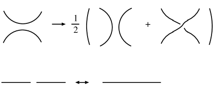
Figure 13: two kinds of elementary local processes

5.2 Linearized loop equations and a free string

Let us consider the all three loop equations eqs. (137), (138) and (139) in the linearized approximation, namely, ignoring the joining and splitting of the loops. Let us first introduce a variable conjugate to $p_{An}$ or $k_{An}$ and that to $\eta_{n}$ or $\zeta_{n}$ by

$$\hat{X}^{A}_{n} = i\frac{\delta}{\delta p_{An}}\;\mbox{or}\;\;i\frac{\delta}{\delta k_{An}}\;\;,$$ (154)

$$\hat{\Psi}_{n} = i\frac{\delta}{\delta\eta_{n}}\;\mbox{or}\;\;i\frac{\delta}{\delta\zeta_{n}}\;\;.$$ (155)

By acting $\hat{X}^{A}_{n}$ and $\hat{\Psi}_{n}$ on a loop, we obtain respectively an operator insertion of $v^{A}$ and that of $\Psi$ at point $n$ on the loop.

Now consider eq. (137) and eq. (138) for the case $X^{r}=v_{M}^{r}$, multiplying them by $p_{nM}^{(1)}$ and $k_{nM}^{(1)}$ respectively. Consistency requires that, for these terms, we must take into account the term from the interactions which represents splitting of a loop with infinitesimal length. This in fact occurs when the splitting point $n$ coincides with the point $n_{1}^{(1)}$ at which $T^{r}$ is inserted. We obtain

$$0 = \frac{1}{g^{2}}p_{nM}^{(1)}\left\langle\left(\delta_{X}\Phi[(1);v_{M}^{r}]\right)\Phi[(2)]\cdots\Phi[(N)]\Psi[(1)]\cdots\Psi[(L)]\right\rangle$$ (156)

$$-\frac{i}{2}2kp_{n}^{(1)2}\left\langle\Phi[(1)]\Phi[(2)]\cdots\Phi[(N)]\Psi[(1)]\cdots\Psi[(L)]\right\rangle\;\;,$$

$$0 = \frac{1}{g^{2}}k_{nM}^{(1)}\left\langle\left(\delta_{X}\Psi[(1);v_{M}^{r}]\right)\Phi[(1)]\cdots\Phi[(N)]\Psi[(2)]\cdots\Psi[(L)]\right\rangle$$ (157)

$$-\frac{i}{2}2kk_{n}^{(1)2}\left\langle\Phi[(1)]\Phi[(2)]\cdots\Phi[(N)]\Psi[(1)]\cdots\Psi[(L)]\right\rangle\;\;.$$

These equations lead to the half of the Virasoro conditions [29]:

$$0 = (p_{n}^{(1)2}+\hat{X}_{n}^{(1)^{\prime}2}+\mbox{(fermionic part)})$$ (158)

$$\left\langle\Phi[(1)]\Phi[(2)]\cdots\Phi[(N)]\Psi[(1)]\cdots\Psi[(L)]\right\rangle\;\;,$$

$$0 = (k_{n}^{(1)2}+\hat{X}_{n}^{(1)^{\prime}2}+\mbox{(fermionic part)})$$ (159)

$$\left\langle\Phi[(1)]\Phi[(2)]\cdots\Phi[(N)]\Psi[(1)]\cdots\Psi[(L)]\right\rangle\;\;,$$

where $\prime$ implies taking a difference between two adjacent points $n$ and $n+1$. The reparametrization invariance of the Wilson loops leads to the remaining half of the Virasoro conditions:

$$0 = (p_{n}^{(1)M}\hat{X}_{nM}^{(1)^{\prime}}+\mbox{(fermionic part)})$$ (160)

$$\left\langle\Phi[(1)]\Phi[(2)]\cdots\Phi[(N)]\Psi[(1)]\cdots\Psi[(L)]\right\rangle\;\;,$$

$$0 = (k_{n}^{(1)M}\hat{X}_{nM}^{(1)^{\prime}}+\mbox{(fermionic part)})$$ (161)

$$\left\langle\Phi[(1)]\Phi[(2)]\cdots\Phi[(N)]\Psi[(1)]\cdots\Psi[(L)]\right\rangle\;\;.$$

Next, let us consider eq. (139), ignoring joining and splitting of the loops. Again consistency appears to require that we drop the cubic terms consisting of $Q$ and $\mbox{\boldmath$Q$}^{\ast}$ in $\delta_{\mbox{\boldmath$Z$}}\Psi[(1);\mbox{\boldmath$Z$}]$ . To write explicitly, the following expression must vanish

$$\left\{\mbox{\boldmath$Q$}^{\ast}_{(f)}(v_{\nu}v^{\nu}+[\Phi_{I},\Phi^{I}])+(\mbox{\boldmath$Q$}\Sigma)_{(f)}F[\Phi_{2}^{\dagger},\Phi_{3}^{\dagger}]+(\mbox{\boldmath$Q$}^{\ast}M^{2})_{(f)}+2(\mbox{\boldmath$Q$}^{\ast}M)_{(f)}v_{4}-i\sqrt{2}\mbox{\boldmath$\psi_{Q}$}^{\ast}_{(f)}\bar{\lambda}\right.$$

$$\left.-\sqrt{2}(\mbox{\boldmath$\psi_{Q}$}\Sigma)_{(f)}F\psi_{\Phi_{1}}\right\}U[k^{(1)}_{.},\zeta^{(1)}_{.};l^{(1)}_{1},l^{(1)}_{0}](\Lambda^{(1)}\mbox{\boldmath$\Pi$}_{f^{(1)}})\approx 0\;\;\;,$$ (162)

$$\left\{\mbox{\boldmath$\psi_{Q}$}^{\ast}_{(f)}\bar{\sigma}^{m}v_{m}+i\sqrt{2}\mbox{\boldmath$Q$}_{(f)}^{\ast}\lambda+\left(\mbox{\boldmath$\psi_{Q}$}\Sigma F(\sqrt{2}\Phi_{1}+M)\right)_{(f)}\right.$$

$$\left.+\sqrt{2}(\mbox{\boldmath$Q$}\Sigma F\psi_{\Phi_{1}})_{(f)}\right\}U[k^{(1)}_{.},\zeta^{(1)}_{.};l^{(1)}_{1},l^{(1)}_{0}](\Lambda^{(1)}\mbox{\boldmath$\Pi$}_{f^{(1)}})\approx 0\;\;\;,$$ (163)

when inserted in

$$\left\langle\Phi[(1)]\Phi[(2)]\cdots\Phi[(N)]\Psi[(2)]\cdots\Psi[(L)]\right\rangle\;\;.$$ (164)

As we stated before, the lefthand sides of eqs. (162) and (163) are expressible as an open loop with some functions of $\hat{X}^{A}_{l^{(1)}_{1}}$ and $\hat{\Psi}_{l^{(1)}_{1}}$ acting on the loop. Let us see by inspection how eqs. (162) and (163) are satisfied by the source functions alone. Consider the following configuration of $\hat{X}_{n}$ and $\hat{\Psi}_{n}\;,$ $n=l^{(1)}_{1}$:

$$\hat{X}^{\mu}\approx 0\;\;\mbox{for}\;\;\mu=0,1,2,3,7\;\;,\;\;\;\hat{X}^{4}=\pm m_{f}\;\;\;.$$ (165)

$$\hat{X}^{{}^{\prime}I}\approx 0\;\;\mbox{for}\;\;I=5,6,8,9$$ (166)

$$\hat{\Gamma}_{3}\hat{\Psi}\approx-\hat{\Psi}\;\;\;,$$ (167)

where $\hat{\Gamma}_{3}\equiv\Gamma_{5}\Gamma_{6}\Gamma_{8}\Gamma_{9}$. Again these equations should be understood in the sense of an insertion at the end point of the open loop.

Eqs. (165), (166), and (167) tell us that the open loop $\Psi[(1)]$ obeys the Dirichlet boundary conditions for $0,1,2,3,4,7$ directions and the Neumann boundary conditions for $5,6,8,9$ directions.

We find that the configuration given by eqs. (165), (166) and (167) solves the linearized loop equations (162), (163). This configuration clearly tells us the existence of $n_{f}$ $D3$ branes and their mirrors each of which is at a distance $\pm m_{f}$ away from the orientifold surface in the fourth direction. This conclusion consolidates both the semiclassical picture in section three and the picture emerging from the fermionic integrations in section four.

References

• [1] H. Itoyama and A. Tokura, Prog. Theor. Phys. 99 (1998)129, hep-th/9708123.
• [2] H. Itoyama and A. Tokura, Phys. Rev. D58 (1998) 026002, hep-th/9801084.
• [3] N. Ishibashi, H. Kawai, Y. Kitazawa and A. Tsuchiya, Nucl. Phys. B498 (1997)467, hep-th/9612115.
• [4] M. B. Green and J. H. Schwarz, Phys. Lett. 149B (1984) 117.
• [5] A. Schild, Phys. Rev. D16 (1977)1722.
• [6] T. Banks, W. Fischler, S. Shenker and L. Susskind, Phys. Rev. D55 (1997) 5112, hep-th/9610043.
• [7] E. Witten, Nucl. Phys. B443 (1995)85.
• [8] H. Itoyama and A. Tsuchiya hep-th/9812177.
• [9] H. Itoyama and T. Matsuo, Phys.Lett. B439 (1998) 46, hep-th/9806139.
• [10] B. Chen, H. Itoyama and H. Kihara, hep-th/9810237.
• [11] U.H. Danielsson and G. Ferretti, Int. J. Mod. Phys. A12 (1997)4581; L. Motl, preprint hep-th/9612198; N. Kim and S.J. Rey, Nucl.Phys. B504 (1997)189.
• [12] S. Kachru and E. Silverstein, Phys. Lett. 396B (1997)70; D. A. Lowe, Nucl.Phys. B501 (1977) 134, Phys. Lett. 403B (1997)243; T. Banks, N. Seiberg and E. Silverstein, Phys. Lett. 401B (1997)30.
• [13] M. B. Green and J. H. Schwarz, Phys. Lett. B151 (1985)21.
• [14] H. Itoyama and P. Moxhay, Nucl. Phys. B293 (1987)685.
• [15] H. Aoki, S. Iso, H. Kawai, Y. Kitazawa and T. Tada, hep-th/9802085.
• [16] T. Hotta, J. Nishimura and A. Tsuchiya, hep-th/9811220
• [17] J. Polchinski, Phys. Rev. Lett. 75 (1995)4724.
J. Polchinski, TASI Lectures on D-branes hep-th/9611050.
• [18] W. Taylor IV, Phys. Lett. 394B (1997) 283 hep-th/9611042; O.J. Ganor, S. Ramgoolam and W. Taylor IV, Nucl. Phys. B492 (1997) 191 hep-th/9611202.
• [19] Y. Arakane, H. Itoyama, H. Kunitomo and A. Tokura, Nucl. Phys. B486 (1997)149.
• [20] N. Seiberg, hep-th/9608011.
• [21] J. Polchinski and E. Witten, Nucl. Phys. B460 (1996)525, hep-th/9510169.
• [22] Y. Arakane and H. Itoyama, in preparation
• [23] C. Vafa, Nucl.Phys. B469 (1996) 403, hep-th/9602022.
• [24] A. Sen, Nucl.Phys. B475 (1996) 562, hep-th/9605150.
• [25] R. I. Nepomechie, Phys. Rev. D31 (1985) 1921.
• [26] M.B. Green, J. H. Schwarz Nucl. Phys. B243 (1984) 475 .
• [27] T. Kugo and T. Takahashi, Prog.Theor.Phys. 99 (1998) 649, hep-th/9711100 ; T. Asakawa, T. Kugo and T. Takahashi, hep-th/9807066.
• [28] L. Brink, J. Scherk and J. H. Schwarz, Nucl.Phys. B121 (1977) 77.
• [29] M. Fukuma, H. Kawai, Y. Kitazawa and A. Tsuchiya, Nucl. Phys. B510 (1998)158, hep-th/9705128.