Supersymmetric Spin Networks and Quantum Supergravity

Abstract

We define supersymmetric spin networks, which provide a complete set of gauge invariant states for supergravity and supersymmetric gauge theories. The particular case of $Osp(1|2)$ is studied in detail and applied to the non-perturbative quantization of supergravity. The supersymmetric extension of the area operator is defined and partly diagonalized. The spectrum is discrete as in quantum general relativity, and the two cases could be distinguished by measurements of quantum geometry.

1 Introduction

In this paper we describe an extension of the spin network states to supergravity. The spin network states play a fundamental role in non-perturbative quantizations of both gauge theories [1, 18] and gravitational theories [2, 3, 4]. In the gauge theory context they provide an orthonormal basis for lattice gauge theories [1, 18]. In this case the spin networks are labeled graphs on the lattice, whose edges are labeled by the finite irreducible representations of the gauge group $G$. In quantum gravity diffeomorphism invariance reduces the degrees of freedom, so that a basis of states invariant under spatial diffeomorphisms and local frame rotations are given by the diffeomorphism classes of spin networks [3, 4]. In this case the group is $SU(2)$, for the chiral formulation based on the Ashtekar-Sen variables [5, 6], or $SU(2)+SU(2)$ in the relativistic case[7, 8].

Over the last ten years there has been a great deal of progress in our understanding of the non-perturbative structure of quantum general relativity, leading to the complete formulation of the quantum theory. Among the key results are the discovery that diffeomorphism invariant observables that measure aspects of the spatial geometry such as areas of surfaces and volumes of regions are finite, and have discrete, computatable spectra[2, 3, 4, 11]. This has led to a physical understanding of the spin network states as eigenstates of these geometrical observables.

During this period there have been a number of papers which extend the methods used to supergravity[12, 13, 14, 15, 16]. These have included the formulation of ${\cal N}=1,2$[13, 14, 15], and ${\cal N}=4$[16] supergravity in terms of chiral, Ashtekar-Sen like variables, as well as the discovery of exact solutions to the quantum constraints[13, 15]. However, much more remains to be done in this direction. The non-perturbative quantization of gravitational theories with extended supersymmetry is largely unexplored territory, despite the fact that extended supersymmetry is essential to the success of string theory, which remains the only successful technique for investigating quantum gravity in the perturbative regime. Another important open area of investigation is the properties of $BPS$ states in the non-perturbative regime. This could be very interesting as it could provide a way to compare results on black hole entropy gotten by both string theory[19] and loop quantum gravity[20].

In this paper we take a first step to the study of the non-perturbative quantization of supersymmetric theories of gravitation by constructing the spin network states for $N=1$ supergravity. We find a number of new features, which suggest that this could be a fruitful direction of investigation. The main result is a diagrammatic method for the construction and evaluation of spin networks for the supergroup $Osp(1|2)$. As a first example we construct and partly diagonalize the supersymmetric extension of the area operator. As expected the spectrum is discrete, but different from that of quantum general relativity. This means that experimental probes of geometry at the Planck scale could in principle distinguish different hypotheses about the local gauge symmetry. This is highly interesting in light of recent developments that suggest that astrophysical probes of Planck scale physics can be developed[21].

Another possible application of the formalism given here is to supersymmetric Yang-Mills theory. It will be very interesting to investigate the extent to which the physics of $N=2$ and $N=4$ super-Yang-Mills theory can be expressed in terms of the spin network states.

It is straightforward to extend the construction here to $N=2$ and higher supersymmetry, this will be described elsewhere [22, 23]. Also, in progress [24] is an examination of the canonical and boundary structure of $N=1,2$ quantum supergravity, which extends results on a holographic formulation of quantum general relativity with finite cosmological constant [25, 8].

In the next section we review some of the basic results about $N=1$ supergravity in chiral coordinates, first studied by Jacobson[12]. In section 3 we present some results from the representation theory of $Osp(1|2)$ which allow us in section 4 to construct quantum spin networks. The diagrammatic method for doing calculations with these states is introduced in section 5, and the following sections describe examples and calculations.

Finally, we mention that we do not here provide rigorous proofs for the assertions made, but we see no reason why a straightforward extension of the rigorous methods introduced in [26, 27, 28, 29] to the present case should not be possible.

2 Review of Quantum Supergravity

Supergravity in terms of the new variables maybe was initially investigated in [12] and extended in [13, 14]. In this paper we will consider mainly $N=1$ supergravity. As shown first by Jacobson in [12], this can be formulated in chiral variables which extend the Ashtekar-Sen variables of general relativity. In this formulation, the canonical variables are the left handed $su(2)$ spin connection $A_{a}^{i}$ and its superpartner spin-3/2 field $\psi_{a}^{A}$. As shown in [15] these fit together into a connection field of the superlie algebra $Osp(1|2)$ (which is referred to in some references [13, 15, 30] as $GSU(2)$.)

We thus define the graded connection:

$$\cal{A}\mit_{a}:=A_{a}^{i}J_{i}+\psi_{a}^{A}Q_{A}$$ (1)

where $a$ is the spatial index. If $\widetilde{E^{a}_{i}}$ and $\pi^{a}_{A}$ are momenta of $A_{a}^{i}$ and $\psi_{a}^{A}$ respectively, we can define the graded momentum as:

$$\cal{E}\mit^{a}:=\widetilde{E^{a}_{i}}J^{i}+\pi^{a}_{A}Q^{A}$$ (2)

The constraints that generate local gauge transformations can then be expressed as usual as,

$${\cal G}_{i}=D_{a}{\widetilde{E^{a}_{i}}}+\frac{i}{\sqrt{2}}\pi^{a}_{A}\psi_{aB}\tau^{AB}_{i}=0$$ (3)

The left and right handed supersymmetry transformations are generated by[12],

$${\cal L}_{A}=D_{a}\pi^{a}_{A}-ig{\widetilde{E^{a}_{i}}}\tau^{B}_{iA}\psi_{aB}=0$$ (4)

$${\cal R}^{A}=\epsilon^{ijk}\widetilde{E^{a}_{i}}\widetilde{E^{b}_{j}}\sigma^{A}_{kB}(-4iD_{[a}\psi^{B}_{b]}+\sqrt{2}g\epsilon_{abc}\pi^{cB})=0$$ (5)

where the cosmological constant is given by $\Lambda=-g^{2}$. The diffeomorphism and hamiltonian constraints can be derived by taking the Poisson Brackets of (4) and (5).

These may be written simply in terms of the fundamental representation of $Osp(1|2)$, which is $3$ dimensional. The superlie algebra $Osp(1|2)$ is then generated by five $3\times 3$ matrices $G_{I}(I=1...5)$, given explicitly in [15]. Using them we can define

$$\cal{A}\mit_{a}^{I}=(A_{a}^{i},\psi_{a}^{A})$$ (6)

$$\cal{E}\mit^{a}_{I}=(\widetilde{E^{a}_{i}},\pi^{a}_{A})$$ (7)

where $I=(i,A)$ labels the five generators of $Osp(1|2)$.

Then the first two constraints can be combined into one $Osp(1|2)$ Gauss constraint:

$$\cal{D}\mit_{a}\cal{E}\mit^{a}_{I}=0$$ (8)

while the last one combines with the Hamiltonian constraint to give:

$$\cal{E}\mit^{a}\cal{E}\mit^{b}\cal{F}\mit_{ab}-ig^{2}\epsilon_{abc}\cal{E}\mit^{a}\cal{E}\mit^{b}\cal{E}\mit^{c}=0$$ (9)

where $\cal{F}\mit_{ab}$ is the curvature of the super connection $\cal{A}\mit_{a}$ :

$$\cal{F}\mit_{ab}:=d_{a}\cal{A}\mit_{b}+[\cal{A}\mit_{a},\cal{A}\mit_{b}]$$ (10)

A key feature of this kind of approach to supergravity is that the supersymmetry gauge invariance has been split into two parts, which play rather different roles. The left handed supersymmetry transformations generated by eq. (4) combine with the $SU(2)$ Gauss’s law (3) to give a local $Osp(1|2)_{L}$ gauge invariance. The theory is then written so that the associated $Osp(1|2)$ connection is the canonical coordinate. The right handed part of the supersymmetry, generated by (5), is a dynamical constraint, being quadratic rather than linear in the momentum. It joins with the Hamiltonian constraint to form a left handed supersymmetry multiplet of dynamical operators.

It is then natural in a chiral formulation of supergravity to represent the left-handed supersymmetry kinematically, and solve it completely by expressing the theory completely in terms of $Osp(1|2)$ invariant states. These are the spin network states we will present shortly. The remaining, right handed, part of the supersymmetry is then imposed as a dynamical operator, and has the same status as the Hamiltonian constraint.

The loop representation for supergravity in the chiral representation was constructed in [15] in terms of $Osp(1|2)$ Wilson loops. These are defined in terms of the supertrace taken in the fundamental $3$ dimensional representation of $Osp(1|2)$.

$$\cal T\mit[\gamma]=Str\cal P\mit exp(\oint_{\gamma}ds\cal A\mit_{a}{\gamma}^{a})\equiv Str{\cal U\mit}_{\gamma}({\cal A\mit})$$ (11)

These Wilson loop states are subject to additional relations arising from intersections of loops. These are solved completely by the introduction of the spin network basis, which are complete and orthogonal[4].

We can construct the loop-momentum variables by inserting the $Osp(1|2)$ invariant momentum $\cal E\mit^{a}$ into the Wilson loops:

$$\cal T\mit^{a}[\alpha](s)=Str[\cal U\mit_{\alpha}(\cal A\mit)\cal E\mit^{a}(\alpha(s)]$$ (12)

It is straightforward to show that the $\cal T\mit[\gamma]$ and $\cal T\mit^{a}[\alpha](s)$ form a closed algebra under Poisson brackets, which we will call the $N=1$ super-loop algebra.

We will also need to describe operators quadratic in the conjugate momenta, which in the loop representation are formed by inserting two momenta in the loop trace,

$$\cal T\mit^{ab}[\alpha](s,t)=Str[\cal U\mit_{\alpha}(s,t)\cal E\mit^{a}(\alpha(t))\cal U\mit_{\alpha}(t,s)\cal E\mit^{b}(\alpha(s))]$$ (13)

The higher order loop operators are similarly defined as

$$\cal T\mit^{ab...c}[\alpha](s,t,...v)=Str[\cal U\mit_{\alpha}(s,t)\cal E\mit^{a}(\alpha(t))\cal U\mit_{\alpha}(t,u)\cal E\mit^{b}(\alpha(u))...\cal U\mit_{\alpha}(v,s)\cal E\mit^{c}(\alpha(s))]$$ (14)

As discussed in [15], the supersymmetric extension of the Chern-Simons state may be formed from the Chern-Simons form of the superconnection ${\cal A}_{a}$,

$$\Psi_{SCS}(\cal{A}\mit_{a})=exp[\frac{i}{2\Lambda}\int d^{3}xSTr(\cal{A}\mit\wedge\cal{F}\mit-\frac{1}{3}\cal{A}\mit\wedge\cal{A}\mit\wedge\cal{A}\mit)]$$ (15)

This state is an exact solution to all the quantum constraints. Like the ordinary Chern-Simons state it also has a semiclassical interpretation as the ground state associated with DeSitter or Anti-DeSitter spacetime.

3 Finite Dimensional Irreducible Representation of $Osp(1|2)$.

Spin networks may be constructed for any Lie or Superlie algebra, $\cal A$ by extending the original definition [17, 18]. An $\cal A$-spin network is a labeled graph whose edges are labeled by the finite dimensional irreducible representations of $\cal A$ and whose nodes are labeled by the associated intertwiners. In quantum gravity spin networks states are associated with the gauge group of the connection, which we have seen in the case of $N=1$ supergravity in the chiral representation [12] to be $Osp(1|2)$. The representation theory of $Osp(1|2)$ has been studied in detail in [30, 31, 32, 34], here we give some of the basic facts that we will need to construct the associated spin network states.

The superlie algebra of $Osp(1|2)$, is constructed by three bosonic generators $J_{i}$ (i=1,2,3)and two fermionic generators $Q_{A}(A=0,1)$. The commutation relations are :

$$[J_{i},J_{j}]=i\epsilon_{ijk}J_{k}$$ (16)

$$[J_{i},Q_{A}]=1/2(\tau_{i})_{A}^{B}Q_{B}$$ (17)

$$\{Q_{A},Q_{B}\}=1/2\epsilon_{AB}\tau^{i}J_{i}$$ (18)

where $\tau^{i}$ are Pauli matrices.

Each irreducible representation of the $Osp(1|2)$ contains two adjacent $SU(2)$ representations. One is labeled by spin $J$ and the other by $J-1/2$. $J$ may be taken as the label of the $Osp(1|2)$ representation, and is related to the eigenvalues of the quadratic Casmier operator of the supergroup $Osp(1|2)$:

$$C=J^{i}J_{i}+\epsilon^{AB}Q_{A}Q_{B}$$ (19)

by

$$\hat{C}|J>=J(J+1/2)|J>$$ (20)

For each $J$ the representation is a graded vector space with a basis labeled by $|J;L;M>$, where J is an integer or half-integer, and L can be $J$ or $J-1/2$ and $-L\leq M\leq L$. The dimension of the space of the representation with spin $J$ is $4J+1$.

The usual rules for combination of angular momentum can be extended directly to these states. The result is a super Racah-Wigner calculus which gives the results of decompositions of products of representations of $Osp(1|2)$. The tensor product is completely reducible and is given by

$$j_{1}\textstyle{\bigotimes}j_{2}=|j_{1}-j_{2}|\textstyle{\bigoplus}|j_{1}-j_{2}+1/2|\textstyle{\bigoplus}...|j_{1}+j_{2}|$$ (21)

Note that this differs from the familiar $SU(2)$ case in that representations which differ from $j_{1}+j_{2}$ by both integers and half integers are included. The Clebsch-Gordon coefficients for the expansion of the basis elements are determined uniquely, from their values for $SU(2)$.

Next we consider the reduction of the tensor product of three irreducible representations $(j_{1},j_{2},j_{3})$. As in the $SU(2)$ case we have two different recoupling schemes. One can couple the representations $(j_{1},j_{2})$ into $j_{12}$ first and then couple the result to $j_{3}$ to give the final representation; or one couples $(j_{2},j_{3})$ into $j_{23}$ first and then couples to $j_{1}$ next. These two representations are related to each other by the Racah sum rule in terms of super rotation 6-symbols. For $Osp(1|2)$, the parity independent super-rotation 6-symbols are defined as[21]:

$${\left\{\begin{array}[]{ccc}j_{1}&j_{2}&j_{12}\\ j_{3}&j&j_{23}\end{array}\right\}}^{s}=(-1)^{\Phi(\lambda_{1},\lambda_{2},\lambda_{3})}{\left\{\begin{array}[]{ccc}j_{1}\lambda_{1}&j_{2}\lambda_{2}&j_{12}\lambda_{12}\\ j_{3}\lambda_{3}&j\lambda&j_{23}\lambda_{23}\end{array}\right\}}^{s}$$ (22)

Then the Racah sum rule reads:

$${\left\{\begin{array}[]{ccc}j_{1}&j_{2}&j_{12}\\ j_{3}&j&j_{23}\end{array}\right\}}^{s}=\sum_{j_{13}}(-1)^{\Theta}{\left\{\begin{array}[]{ccc}j_{1}&j_{3}&j_{13}\\ j_{2}&j&j_{23}\end{array}\right\}}^{s}{\left\{\begin{array}[]{ccc}j_{2}&j_{1}&j_{12}\\ j_{3}&j&j_{13}\end{array}\right\}}^{s}$$ (23)

In a similar way the Biedenharn-Elliott identity can be constructed for the super 6-j symbols:

$${\left\{\begin{array}[]{ccc}j_{1}&j_{2}&j_{12}\\ j_{3}&j_{123}&j_{23}\end{array}\right\}}^{s}{\left\{\begin{array}[]{ccc}j_{23}&j_{1}&j_{123}\\ j_{4}&j&j_{14}\end{array}\right\}}^{s}$$ (28)

$$=\sum_{j_{124}}(-1)^{\theta_{be}}{\left\{\begin{array}[]{ccc}j_{2}&j_{1}&j_{12}\\ j_{4}&j_{124}&j_{14}\end{array}\right\}}^{s}{\left\{\begin{array}[]{ccc}j_{3}&j_{12}&j_{123}\\ j_{4}&j&j_{124}\end{array}\right\}}^{s}{\left\{\begin{array}[]{ccc}j_{14}&j_{2}&j_{124}\\ j_{3}&j&j_{23}\end{array}\right\}}^{s}$$ (35)

where $\theta_{be}$ and $\Theta$ are the sign factors related to the super-spins involved. The interesting fact is that except these two sign factors, the structure of two relations are the same as the structure for SU(2) rotation algebra. Therefore when we restrict the sum of three super-spins in all the triangles $(j_{1},j_{2},j_{12})$, $(j_{1},j_{3},j_{13})$, $(j_{2},j_{3},j_{23})$ to be integers, then all the expressions go back to the normal racah sum rule and the Biedenharn-Elliott identity for $SU(2)$.

4 Spin Network States of $N=1$ Supergravity

We recall that a spin network state of quantum general relativity, denoted $|\Gamma>$ consists of an embedding of closed graph $\Gamma$ into a fixed three manifold $\Sigma$ with edges labeled by the representation of SU(2)($SU(2)_{q}$) and vertices labeled by intertwining operators, namely distinct ways to decompose the incoming representations into a singlet. Here we define the super spin networks in the same way only by replacing the $SU(2)$ with superlie algebra $Osp(1|2)$. The elements of the super spin networks are links and vertices. Notice that in quantum general relativity, the link of color $n$ corresponds to a parallel propogator of connection $A_{a}$ along this path in the spin n/2 representation of su(2), here associated to very link we also label a color $n_{i}$ which is two times as the superspin $j_{i}$ which labels the representation of $Osp(1|2)$. For every vertex $v_{e}$, there are incoming links with color $n^{in}_{ei}$ and outcoming links with color $n^{out}_{ei}$. so we can label the vertex by the total color $v_{e}=\sum_{i}n^{in}_{ei}-\sum_{i}n^{out}_{ei}$ which satisfies $1/2\leq v_{e}\leq k/2$.

Corresponding to every super spin network $(\Gamma^{sg},n_{i},v_{e})$, there is a super spin network state $<\Gamma^{sg},n_{i},v_{e}|$ in the Hilbert space of the supergravity. As an independent basis, the super spin network can also be expressed as the bras so that a general state in this representation is given by:

$$\Psi[\Gamma^{sg}]:=<\Gamma^{sg}|\Psi>$$ (36)

We now list some basic facts about the super spin networks .

• As in the $SU(2)$ case there is no intertwiner associated to trivalent nodes because given

  $$|J_{1}-J_{2}|\leq J_{3}\leq|J_{1}+J_{2}|$$ (37)

  then the map from the tensor products of two representations to the reduced representation is unique.

• The condition that the sum of three colors of the links adjacent to a trivalent vertex must sum to an even number does not hold, because both even and odd spins appear in the sum (21). As the color of the link is twice the spin, the edges of a trivalent vertex can be any integers such that eq. (37) holds.

• If the valences adjacent to the same vertex is more than three, intertwiners are needed to label the different maps from the incoming representations to the singlet state. As in the $SU(2)$ case the multi-valent vertices can be decomposed in terms of trivalent vertex connected by internal edges, as described in [4].

Note that this means that there is no simple way to decompose the $Osp(1|2)$ spin networks completely in terms of ordinary spin networks because there is no ordinary spin network vertex corresponding to the superspin network vertices where the sum of incident colors is odd. However, there is still a very useful decomposition, which we will give below.

As in the $SU(2)$ case, there is a recoupling theory based on the Racah sum rule and Biedenharn-elliott identity in terms of the super-rotation 6-j symbols. We can express the recoupling theory by fig.1:

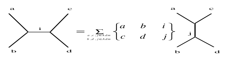
Figure 1: Recoupling theory for $Osp(1|2)$ 6-j symbols

Where the sum is over labels such that the super 6-j symbols satisfies the triangle inequalities eq. (37).

5 Graphic Representation of the Super Spin Networks

We can now give a diagrammatic notation for $Osp(1|2)$ spin networks which is useful for computation. We follow the method developed in [4] and elaborated in [11] for quantum general relativity in which a diagrammatic notion for $SU(2)$ spin network states was developed by modifying notations used by Penrose[17] and Kauffman and Linns[35]. The result is a diagrammatic notation of super spin networks based on the connection between them and the representation theory of the supergroup $Osp(1|2)$.

5.1 Element of the Diagrams

The basic fact about the $SU(2)$ representation theory on which the Penrose and Kauffman and Linns notation rests is that all irreducible representations can be obtained by symmetrizing products of the fundamental representation. In the case of $Osp(1|2)$ all irreducible representations can be obtained via a process of graded symmetrizing, in which there are extra signs for even and odd parts of the representations. There are in fact two different fundamental representations for the $Osp(1|2)$, which are complex conjugates of each other. Let us consider first the left handed fundamental representation. It is a three dimensional graded vector space, whose elements may be written

$$\xi_{\alpha}=(\begin{array}[]{c}\psi_{A}\\ \phi_{\circ}\end{array})$$ (38)

where $A=(0,1)$ denotes the left handed $SU(2)$ spinor index part and $\alpha=\circ$ denotes the third component. Here we take the $\xi_{A}=\psi_{A}$ to be fermionic while the $\xi_{\circ}=\phi$ is bosonic. The grade of the index, $g(\alpha)$, is defined to be one for $\circ$ and zero for $A$. Under the action of $Osp(1|2)$, $\xi_{\alpha}$ transforms as:

$$\xi_{\alpha^{\prime}}={U_{\alpha^{\prime}}}^{\alpha}\xi_{\alpha}$$ (39)

where $3\times 3$ matrix $U_{\alpha^{\prime}}^{\alpha}$ is an element in the fundamental representation of $Osp(1|2)$.

The higher irreducible representations are formed by taking graded symmetric products of this fundamental representation. For instance the basis states for J=1 span a five dimensional space, which can be constructed by symmetrized tensor products of two states in the fundamental representation, as,

$$\xi_{(\alpha\beta)}:=\frac{1}{2}[\xi_{\alpha}\xi_{\beta}+(-1)^{g(\alpha)g(\beta)}\xi_{\beta}\xi_{\alpha}]$$ (40)

We can then read off the components of the basis states of the $J=1$ representation. They consist of a pair of $SU(2)$ representations, given by,

$$\xi_{(\alpha\beta)}=(\xi_{(AB)},\xi_{(A}\phi_{\circ)})$$ (41)

The first term is the bosonic component defined as,

$$\xi_{(AB)}=\frac{1}{2}(\psi_{A}^{(1)}\psi_{B}^{(2)}+\psi_{B}^{(1)}\psi_{A}^{(2)})$$ (42)

and the second term is the fermionic component of the basis states.

$$\xi_{(A}\phi_{\circ)}=\frac{1}{2}(\psi_{A}^{(1)}\phi_{\circ}^{(2)}+\phi_{\circ}^{(1)}\psi_{A}^{(2)})$$ (43)

The other term $\phi_{[\circ\circ]}$ vanishes due to the antisymmetrization.

Under the action of $Osp(1|2)$, the states transform as:

$$\xi_{(\alpha^{\prime}\beta^{\prime})}={U_{(\alpha^{\prime}\beta^{\prime})}}^{(\alpha\beta)}\xi_{\alpha\beta}$$ (44)

where:

$${U_{(\alpha^{\prime}\beta^{\prime})}}^{(\alpha\beta)} = \frac{1}{2}[(-1)^{g(\alpha)[g(\beta^{\prime})-g(\beta)]}{U_{\alpha^{\prime}}}^{\alpha}{U_{\beta^{\prime}}}^{\beta}$$ (45)

$$+(-1)^{g(\alpha^{\prime})g(\beta^{\prime})}(-1)^{g(\alpha)[g(\alpha^{\prime})-g(\beta)]}{U_{\beta^{\prime}}}^{\alpha}{U_{\alpha^{\prime}}}^{\beta}]$$

If we only consider the unit element of $Osp(1|2)$ in this representation, then we have

$${\delta_{(\alpha^{\prime}\beta^{\prime})}}^{(\alpha\beta)}=\frac{1}{2}[{\delta_{\alpha^{\prime}}}^{\alpha}{\delta_{\beta^{\prime}}}^{\beta}+(-1)^{g(\alpha^{\prime})g(\beta^{\prime})}{\delta_{\beta^{\prime}}}^{\alpha}\delta_{\alpha^{\prime}}^{\beta}]$$ (46)

This allows us to generalize the Penrose diagrammatic notation for $SU(2)$ spin networks. We indicate the elements of a super spin networks by bold lines, the elements with su(2) indices by thin lines and third component $\phi=\xi_{\circ}$ by dotted lines. Then we can denote the $\delta_{\alpha^{\prime}}^{\alpha}$ and its components as fig.2.

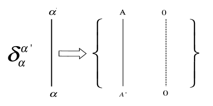
Figure 2: Unit element in fundamental representation of $Osp(1|2)$

Then it’s straightforward to express (35) as fig.3.

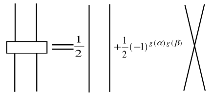
Figure 3: Construction of unit element in representation with spin one

Let us consider the component formulation of this expression. When the indices of delta are $SU(2)$ spinor indices, it’s easy to see that it goes back to the normal spin networks expression. If one index is fermionic and the other one is bosonic, they commute with other and we can denote the expression by two vertical lines, one solid and one dotted. If both indices are bosonic, which may be denoted by two vertical dotted lines. However this term vanishes because the graded symmetrization antisymmetrizes them and there is a single bosonic component. The procedure of the decomposition of the super element can then be drawn as fig.4.

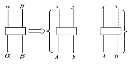
Figure 4: Decomposition of the link with color 2 in super spin networks into normal SU(2) ones

Thus, we have a way to decompose the diagrams for $Osp(1|2)$ spin networks into combinations of $SU(2)$ spin network diagrams and dotted lines representing the single bosonic component of the fundamental representation. It is straightforward to see how this works when applied to any higher dimensional representation of $Osp(1|2)$, which is gotten by making a graded symmetrization of $n$ fundamental representations. The basic property is that all the terms whose corresponding graphs have two or more dotted lines must vanish also since we need to antisymmetrize them. As a result, the basis states in any dimensional representation consists of two components,

$$\xi_{(\alpha_{1}...\alpha_{n})}=(\xi_{(A_{1}...A_{n})},\xi_{(A_{1}...A_{n-1}0)}),$$ (47)

where

$$\xi_{(A_{1}...A_{n})}=\psi_{(A_{1}}\psi_{A_{2}}...\psi_{A_{n})}$$ (48)

$$\xi_{(A_{1}...A_{n-1}0)}=\psi_{(A_{1}}\psi_{A_{2}}...\psi_{A_{n}-1}\phi_{0)}.$$ (49)

The unit element of the supergroup in this representation can be expressed as:

$${\delta_{(\alpha^{\prime}\beta^{\prime}...\gamma^{\prime})}}^{(\alpha\beta...\gamma)}:={\delta_{(\alpha^{\prime}}}^{\alpha}{\delta_{\beta^{\prime}}}^{\beta}...{\delta_{\gamma^{\prime})}}^{\gamma}$$ (50)

and the corresponding graph can be drawn as fig.5. Thus we see that we can decompose a super spin network into a sum of diagrams, each of which is a normal spin network together with dotted lines. In this decomposition each edge of the superspin network, with color $n$ becomes two ordinary spin network edges, the first an $n$ line without a dotted line and the second with an $n-1$ line with a single dotted line. This is shown in fig.5.

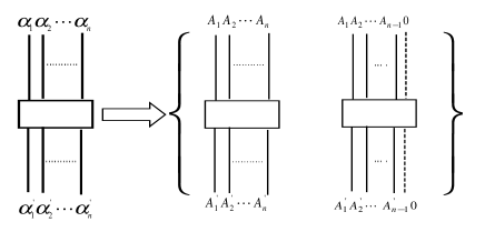
Figure 5: Decomposition of the super link of color $n$

5.2 Trivalent Vertices

Next we consider the tri-valent vertex. As there is no restriction that the incident colors must add up to an even number, as in the $SU(2)$ case, the simplest trivalent node is the one in which all three edges have color one. This node can be visualized in two ways, depending on how the direction of time is read. One fermion with spin one half meets one boson with spin zero and then changes into one fermion, or two fermions with spin one half meet together forming into a boson which is also singlet state. These processes are expressed by fig.6.

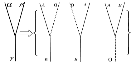
Figure 6: The three terms in the decomposition of the trivalent vertex, in the case that all colors are equal to one.

We next consider the case in which every link has color two. This can be decomposed into the ordinary $SU(2)$ spin networks as shown in fig.7.

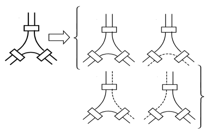
Figure 7: Decomposition of trivalent vertex in which every link has color two.

In general, if the sum of the three colors is even it can be decomposed into four terms, each of which contains an ordinary spin network plus, possible dotted edges. We illustrate it in fig.8.

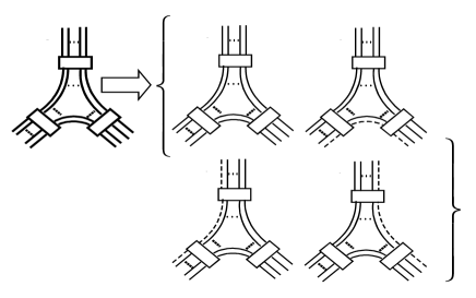
Figure 8: Decomposition of trivalent vertex in which the sum of colors is even

5.3 Simple Closed Diagrams: the Super-$\Theta$ Graph

We have found that edges and nodes of superspin networks decompose into sums of terms, each of which consists of an ordinary spin network, perhaps dressed by dotted lines. As a result any closed super spin network can be decomposed into a sum of such terms. As an example, we describe the simplest example of a closed spin network, which is the $\Theta$ graph. The simplest one is the diagram in which every link has color one. This super $\Theta$ graph can be decomposed into a sum of three components, each of which is an ordinary spin network. This is illustrated in fig.9.

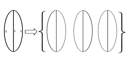
Figure 9: Decomposition of the simplest $\Theta$ graph

Another interesting $\Theta$ diagram is the one in which the colors of three links are $(n,2,n)$. We will use it later in the calculation of the area spectrum in quantum supergravity. It can be decomposed into four components in terms of $SU(2)$ spin networks as shown in fig.10.

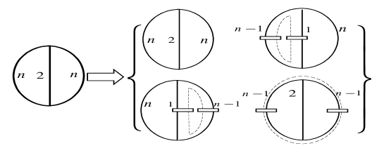
Figure 10: The general case of the decomposition of $\Theta$ graph

6 Evaluation of Super Spin Networks

In the case of $SU(2)$ spin networks, the edges represent projection operators, which live in the Temperly Lieb algebra. These can always be decomposed using the bracket identity [see fig.11].

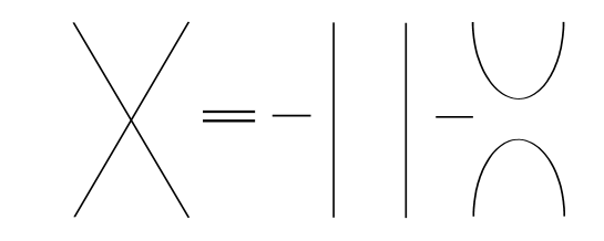
Figure 11: The bracket identity for $SU(2)$ spin networks

As a result, associated with any ordinary spin network there is a number which is called its evaluation. This was first introduced by Penrose[17]. It is now known to be a special case of the Kauffman bracket polynomial when the quantum deformation parameter $A=\pm 1$.

For the supergroup $Osp(1|2)$, the spinor identity does not exist any more. Therefore there is no bracket identity (although in the super loop representation some identities analogous to the Mandelstam identity can be expressed by means of the supertraces of the holonomies [15]). But we can still evaluate a super spin networks by first decomposing it into ordinary $SU(2)$ spin networks, using the rules defined in the previous section, and then evaluating each component.

The evaluation of a super spin network in fact corresponds to taking the supertrace of a product of projection operators on the direct product of a number of fundamental representations. The fact that it can be expressed in terms of the evaluations of ordinary spin network is a consequence of the fact that the supertrace can be decomposed into a sum of traces over the $SU(2)$ representations that make up a representation of $Osp(1|2)$. In fact, the sign factors necessary to turn a sum of traces into a supertrace are already built into our formalism by the sign factors that go into the graded symmetrizations that define the edges and nodes of the super spin networks. In the example of the super $\Theta$ graph, as well as in the examples that follow, one can see how this works explicitly.

As a direct application, we can calculate the super standard closure of the super tangles, which is defined as the supertrace of the holonomy of the flat connection in this representation:

$$Str_{j}(\delta_{\alpha_{1}\alpha_{2}...\alpha_{n}}^{\alpha^{\prime}_{1}\alpha^{\prime}_{2}...\alpha^{\prime}_{n}}) = tr_{j}(\delta_{A_{1}A_{2}...A_{n}}^{A^{\prime}_{1}A^{\prime}_{2}...A^{\prime}_{n}})+tr_{j}(\delta_{A_{1}A_{2}...A_{n-1}0}^{A^{\prime}_{1}A^{\prime}_{2}...A^{\prime}_{n-1}0})$$ (51)

$$= (-1)^{(2j)}(2j+1)+(-1)^{2(j-1/2)}[2(j-1/2)+1]$$

$$= (-1)^{2j}$$

Here when we take the trace of the dotted line, we find its value is one.

Let us consider the simple super $\Theta$ graph in which the colors of links are $(1,2,1)$. After decomposing the graph into the normal spin networks and taking the trace of them as shown in fig.12, we find the value of the $\Theta$ graph is one.

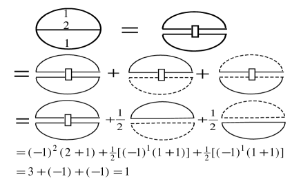
Figure 12: The Evaluation of $\Theta(1,2,1)$

Also since this graph is equivalent to the super standard closure with color two (see the first step in figure 12), we can find the value of this graph by (40) directly, in which $n$ equals two. If we consider another example in which the colors are (2,2,2), we have the answer illustrated in fig.13.

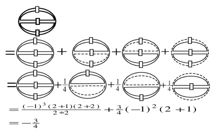
Figure 13: The Evaluation of $\Theta(2,2,2)$.

In the third step the coefficient one fourth appears when we try to separate the dotted loop from the real-line loops. Since initially the bosonic index is symmetrized with the fermionic indices, we have four different ways to connect the ropes to form loops. But the value of any loop which is formed by connecting one real rope and one dotted rope must be zero, therefore only one graph has non-zero value. We illustrate the specific expansion in fig.14.

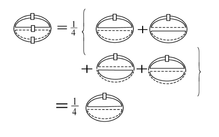
Figure 14: Separation of the dotted loop from the $\Theta$ graph

The most interesting $\Theta$ graph, which has important application to the calculation of the area spectrum in supergravity, is the one with colors (n,2,n). From the last section, we see this graph can be divided into four graphs with respect to the ordinary su(2) spin networks. In fig.16 the bosonic index is symmetrized with the fermionic indices. To evaluate all these graphs, we also need to separate the dotted loop from each $\Theta$ graph. In other words, we must decouple the dotted line from the symmetrizer just as we have done for the $\Theta$ graph (1,2,1)and (2,2,2).

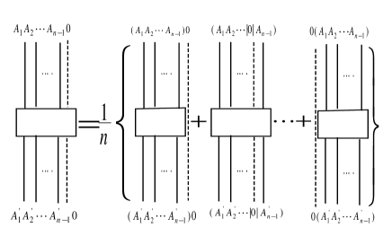
Figure 15: Separation of the dotted line from the symmetrizer.

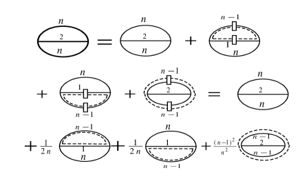
Figure 16: Evaluation of the $\Theta$ graph with color (n,2,n)

When doing this one must be careful to obtain the right coefficients for each term. The key point is that the dotted line has to be connected to the dotted line and for every vertex the triangle inequality must hold. In general when the dotted line is separated from the symmetrizer of color $n$, the factor $1/n$ appears and there are $n$ terms due to the different permutation of the dotted line as shown in fig.15. For the second and third term in figure 16, there is only one possible routing of the dotted line which has non-zero value among the $2n$ possibilities, therefore the coefficients are $1/2n$. For the last term, the dotted line can’t be connected to the link of color two so there are $(n-1)(n-1)$ routings with non-zero value and the coefficient is $(n-1)^{2}/n^{2}$. Now it’s straightforward to evaluate the super $\Theta$ graph by summing all the ordinary $\Theta$ graphs:

$$\Theta(n,2,n) = \frac{(-1)^{n+1}(n+1)(n+2)}{2n}+\frac{1}{2n}(-1)^{n}(n+1)$$ (52)

$$+\frac{1}{2n}(-1)^{n}(n+1)+\frac{(n-1)^{2}}{n^{2}}\frac{(-1)^{n}n(n+1)}{2(n-1)}$$

$$= \frac{(-1)^{(n+1)}(n+1)}{2n}$$

It is not difficult to generalize this calculation to the case in which the super $\Theta$ graph has color$(m,2,n)$. One finds that the coefficients before every ordinary $\Theta$ graphs respectively are $(1,1/2n,1/2m,(n-1)(m-1)/mn)$. However, it is more complicated to find a general formula for the super $\Theta$ graph with color $(m,n,p)$, in which the separation of the dotted loop from links labeled by $m,n$ obviously depends on the third link with color $p$.

7 The Super-area Operator and Its Spectrum

A natural question concerning the spin network states of supergravity is whether we can construct observables such as the area and the volume of the space in terms of their action on super spin network states, as in the case of general relativity[4]. Here we show that the answer is yes, if the operator is suitably defined. In this section we construct the area operator and calculating its eigenvalues in the context of super spin network basis.

The gauge invariance of supergravity includes the $Osp(1|2)$ symmetry, hence we must require the observables should be invariant under its full action. The expression for the area operator in quantum general relativity, computed in [2, 3, 4], is not an observable in supergravity, since it is not $Osp(1|2)$ gauge invariant. But it is not difficult to extend the definition of the area of a surface in general relativity to an expression which is $Osp(1|2)$ invariant. Given a spatial surface $\cal S\mit$, which is a two-dimensional manifold embedded in the spacetime manifold $\cal M\mit$, we define the supersymmetric area to be:

$$A[\cal S\mit]=\int_{\cal s\mit}d^{2}s\sqrt{n_{a}n_{b}\cal E\mit^{aI}\cal E\mit^{b}_{I}}$$ (53)

where $n_{a}$ is the normal vector of the surface and the ${\cal E}^{aI}$ is the conjugate momentum. The definition of area operator is closely related to the two-hand loop operator $\cal T\mit^{ab}$ that we have introduced in section three. When the loop shrinks to a point, following [11] and using the identity about the supertrace of the $Osp(1|2)$ Lie algebra we find,

$$\cal T\mit^{ab}[\alpha](s,t)=Str[\cal U\mit_{\alpha}(s,t)\cal E\mit^{a}(\alpha(t))\cal U\mit_{\alpha}(t,s)\cal E\mit^{b}(\alpha(s))]=2\cal E\mit^{aI}\cal E\mit^{b}_{I}$$ (54)

As a result, the area of the small surface with side L, to zeroth order, can be written as,

$$A[\cal S\mit]=\lim_{L\rightarrow\infty}\sum_{I}\sqrt{A_{I}^{2}}$$ (55)

where:

$$A_{I}^{2}=\frac{1}{2}\int_{s_{I}}d^{2}\sigma\int_{s_{I}}d^{2}\tau n_{a}(\sigma)n_{b}(\tau)\cal T\mit^{ab}[\alpha_{\sigma\tau}](\sigma,\tau)$$ (56)

Now we define the $Osp(1|2)$ invariant area operator to be,

$$\hat{A}[{\cal S}]=\lim_{L\rightarrow\infty}\sum_{I}\sqrt{\hat{A}_{I}^{2}}$$ (57)

where,

$$\hat{A}_{I}^{2}=\frac{1}{2}\int_{s_{I}}d^{2}\sigma\int_{s_{I}}d^{2}\tau n_{a}(\sigma)n_{b}(\tau)\hat{\cal T}^{ab}[\alpha_{\sigma\tau}](\sigma,\tau)$$ (58)

Next we want to consider the action of the area operator on spin network states. In [3, 11], the discrete spectrum of the area operator in spin network states is worked out in different ways. One can divide the link, the element of the spin networks, into ropes in loop representation so that the area operator acts on the state as a second order loop operator which can be expressed in terms of the elementary grasp operation; or equivalently one can define the action of the area operator on spin networks as inserting two trivalent intersections on the link by a new link of color $2$, then calculate the eigenvalues of the operator by recoupling theory directly. Here we can define the action of super $\cal T\mit$ variables in terms of the elementary grasp operation. This allows us to calculate the spectrum of the operator in both ways.

Let us consider the former method first. The action of the super operator $\cal T\mit^{a}$ on the super spin networks can be defined as fig.(17).

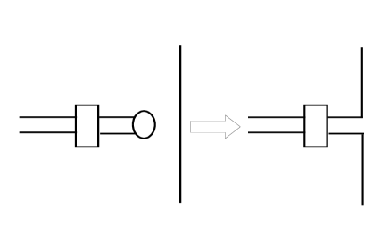
Figure 17: Action of $\cal T\mit^{a}$ with one grasp on the super spin networks

Basically as we have done in the previous sections, we can decompose super spin networks into the ordinary SU(2) ones and then consider the action of the operator on them separately. From fig.4, we see the super link of color 2 can be divided into two components, so the corresponding action of the super operator can be divided into two parts which can be illustrated in figure 18. For convenience, let’s define these actions as “real grasp” and “dotted grasp” respectively.

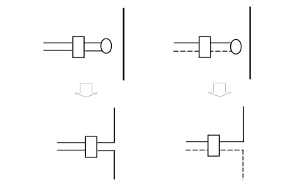
Figure 18: The super grasps in the view of ordinary SU(2) spin networks

When decomposed in terms of $SU(2)$ spin networks, we find that there are several distinct grasp operations. The first possibility is the real grasp to the real line, which is exactly the normal grasps having appeared in [11]. The second one is the dotted grasp acting on the real line, and the third one the dotted grasp acting on the dotted line. Note that the real grasp acting on the dotted line vanishes since the only possible result is that two real lines combine together and go back.

Now it’s straightforward to express the action of super operators on the link of color n, but we need be careful to determine the multiplicative factors when using the Leibnitz rule to define the action of area operator on it. Specially, there is a great difference between the real grasp and the dotted grasp. Since the area operator is related to the second order super loop operator, we can take the $\cal T\mit^{ab}$ as the handle with two grasps in the super spin network basis. When two grasps act on the link of color $n$, they can grasp the same rope, or any two different ropes, so there are $n^{2}$ possible ways to grasp the link. But when the real grasps act on the dotted rope, the results of the action are zero. So the number of “non-zero” grasps are $n^{2}$ and $(n-1)^{2}$ to the doublet of the super link respectively. Also after the two dotted grasps act on the link of color $n$, we need separate the dotted rope from the solid ropes so that we can apply the formula with respect to the ordinary $SU(2)$ spin networks. As we have discussed in the last section, the separation involves the factor $1/2n$. As a result the coefficients before the graphs acted by the dotted grasps are $n/2$. Figure 19 and 20 show the actions of these two kinds of grasps on the link of color n.

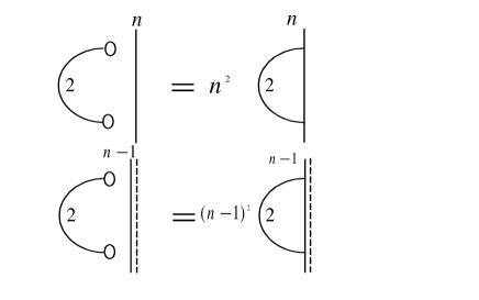
Figure 19: Action of the second order real grasp

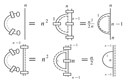
Figure 20: Action of the second order dotted grasp

Finally we arrive at the last step of this section, that is to calculate the spectrum of the area operator. Combining the two actions of the grasps together, we find the super spin network states are the eigenstates of the $\hat{A}^{2}$. It is straightforward to compute the eigenvalues of $\cal T\mit^{ab}$ in the super spin network basis (see fig.21) and the result is:

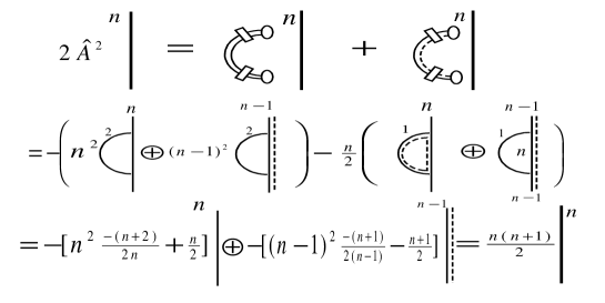
Figure 21: The action of the area operator

$$\hat{A}^{2}|\Gamma^{sg},n_{i},v_{e}>=\sum_{i}\frac{n_{i}(n_{i}+1)}{4}l_{p}^{4}|\Gamma^{sg},n_{i},v_{e}>$$ (59)

Where $l_{p}$ is Planck length. As a result we find that the eigenvalues of the area operator are given by,

$$\hat{A}|\Gamma^{sg},n_{i},v_{e}>=\sum_{i}\sqrt{\frac{n_{i}(n_{i}+1)}{4}}l_{p}^{2}|\Gamma^{sg},n_{i},v_{e}>=\sum_{i}\sqrt{j_{i}(j_{i}+\frac{1}{2})}l_{p}^{2}|\Gamma^{sg},n_{i},v_{e}>$$ (60)

Here we have applied the identities and the formulas in SU(2) spin networks. This confirms the expected result that the spectrum is discrete and is directly related to the eigenvalues of the Casmier operator of $Osp(1|2)$.

Next we conclude that we can get the same solution to eigenvalues of the area operator directly by employing the identity associated with the representation of $Osp(1|2)$, in which the evaluation of the super projectors eq.(51) and super $\Theta$ graphs (52) is involved. The procedure is shown in fig.22.

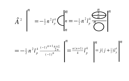
Figure 22: The evaluation of area spectrum by means of the identity for super spin networks

Finally, we note that we have computed here only a part of the spectrum of the superarea operator, which is that concerned with the intersections of edges of the superspin network with the surface $S$. As in the $SU(2)$ case there are additional eigenvalues associated with the possibility that the surface $S$ intersects nodes of the superspin network. These eigenvalues may not be physically relevant as the probability of such intersections is zero, but in any case they can be computed directly.

8 Conclusions

In this paper we have taken an important step in the extension of the results of loop quantum gravity to supergravity and string theory. We have shown that for ${\cal N}=1$ supergravity in $3+1$ dimensions there is a straightforward extension of the methods developed in [3, 4, 11] from quantum general relativity. The extension to ${\cal N}=2$ is in progress and will be reported shortly [22, 24]. There is in fact nothing to prevent the direct extension to any $\cal N$, what is difficult is only the question of whether, for ${\cal N}>2$, all the degrees of freedom of higher $\cal N$ supergravities are represented by an extension of the connection representation, or whether additional degrees of freedom need to be introduced. In this connection we may note that the extension of the loop representation to represent the states of $p$-form gauge fields is straightforward, and has been worked out for $p=2$ [36, 37] and $p=3$ [38]. In the latter case an extension of the loop representation that describes a limit of $\cal M$ theory in which only the $3$-form field of $11$ dimensional supergravity survives can be discussed, and a large set of exact non-perturbative states found [38].

Finally, the quantum deformation of the supersymmetric spin network states may be developed along the lines of [35], and applied both to yield the supersymmetric extension of the spin foam models[7, 39] as well as to the background independent formulation of $\cal M$ theory described in [40, 41].

References

- [1] J. Kogut and L. Susskind, Hamiltonian formulation of Wilson’s lattice gauge theories, Phys. Rev. D11: 395,1975.
- [2] L. Smolin, in Quantum Gravity and Cosmology, eds J Pérez-Mercader et al, World Scientific, Singapore 1992; The future of spin networks, gr-qc/9702030 in the Penrose Feshscrift.
- [3] C. Rovelli and L. Smolin, Discreteness of area and volume in quantum gravity, Nuclear Physics B 442 (1995) 593. Erratum: Nucl. Phys. B 456 (1995) 734.
- [4] C. Rovelli and L. Smolin, Spin networks and quantum gravity, Physical Review D 52 (1995) 5743-5759, gr-qc/9505006.
- [5] A. Sen, Gravity as a spin system, Phys. Lett. B119 (1982) 89; Quantum theory of a spin 3/2 system in Einstein spaces, Int. J. of Theor. Phys. 21 (1982) 1.
- [6] A. Ashtekar, Phys. Rev. Lett. 57 (1986) 2244; Phys. Rev. D36 (1987) 1587.
- [7] J. Barrett and L. Crane, Relativistic spin networks and quantum gravity, J. Math. Phys.39(1998) 3296-3302, gr-qc/9709028.
- [8] L. Smolin, Holographic formulation of quantum general relativity, hep-th/9808191.
- [9] C. Rovelli, Loop Quantum Gravity, Review paper written for the electronic journal ‘Living Reviews’, gr-qc/9710008.
- [10] L. Smolin, The future of spin networks, in the Penrose Feshscrift, gr-qc/9702030.
- [11] R. Loll, Nucl. Phys. B444 (1995) 619; B460 (1996) 143; R. DePietri and C. Rovelli, Geometry eigenvalues and scalar product from recoupling theory in loop quantum gravity, gr-qc/9602023, Phys. Rev. D54 (1996) 2664; Simonetta Frittelli, Luis Lehner, Carlo Rovelli, The complete spectrum of the area from recoupling theory in loop quantum gravity, gr-qc/9608043; R. Borissov, Ph.D. thesis, Temple, (1996).
- [12] T. Jaocobson, New variables for canonical supergravity Class. Quant. Grav. 5 (1988) 923.
- [13] T. Sano, J. Shiraishi, The Non-perturbative Canonical Quantization of the N=1 Supergravity, Nucl. Phys. B410(1993) 423, hep-th/9211104; H. Kunitomo, T. Sano, The Ashtekar formulation for Canonical N=2 Supergravity Int. J. Mod. Phys.D1(1993)559; The Ashtekar formalism and WKB Wave Functions of N=1,2 Supergravities, hep-th/9211103. H. Kunitomo and T. Sano The Ashtekar formulation for canonical N=2 supergravity, Prog. Theor. Phys. suppl. (1993) 31; T. Sano and J. Shiraishi, The Non-perturbative Canonical Quantization of the N=1 Supergravity, Nucl. Phys. B410 (1993) 423, hep-th/9211104; The Ashtekar Formalism and WKB Wave Functions of N=1,2 Supergravities, hep-th/9211103; K. Ezawa, Ashtekar’s formulation for N=1,2 supergravities as “constrained” BF theories , Prog. Theor. Phys.95(1996) 863-882, hep-th/9511047.
- [14] K. Ezawa, Ashtekar’s formulation for N=1,2 supergravities as “constrained” BF theories, Prog. Theor. Phys.95(1996) 863-882, hep-th/9511047.
- [15] D. Armand-Ugon, R. Gambini, O. Obregon, J. Pullin, Towards a loop representation for quantum canonical supergravity, Nucl. Phys. B460(1996) 615-631, gr-qc/9508036; R. Graham, C. Csordas, Exact quantum state for N=1 supergravity, Phys. Rev. D52(1995) 6656-6659, gr-qc/9507008.
- [16] T. Kadoyoshi and S. Nojiri, N=3 and N=4 two form supergravities, Mod. Phys. Lett. A12: 1165-1174,1997, hep-th/9703149; L. F. Urrutia Towards a loop representation of connection theories defined over a super-lie algebra, hep-th/9609001.
- [17] R.Penrose, The theory of quantized directions, in Quantum theory and beyond, ed T.Bastin, Cambridge U Press 1971.
- [18] J. Baez, Spin Networks in Nonperturbative Quantum Gravity, in The Interface of Knots and Physics, ed. Louis Kauffman, A.M.S. Providence,1996, 167-203, gr-qc/9504036; Spin Network States in Gauge theory, Adv. Math. 117(1996)253-272, gr-qc/9411007.
- [19] J. Maldacena, Black Holes in String Theory, hep-th/9607235; A. W. Peet, The Bekenstein Formula and String Theory, Class. Quant. Grav.15(1998) 3291-3338, hep-th/9712253; G. T. Horowitz and J. Polchiski, Correspondence Principle for Black Holes and Strings, Phys. Rev. D55, 6189(1997).
- [20] K. Krasnov, gr-qc/9603025, Phys.Rev. D55 (1997) 3505-3513; gr-qc/9605047, Gen. Rel. Grav. 30 (1998) 53-68; A. Ashtekar, J. Baez, A. Corichi, K. Krasnov, Phys. Rev. Lett. 80 (1998) 904-907, gr-qc/9710007; K. Krasnov, Class. Quant. Grav.16(1999)L15-L18, gr-qc/9902015.
- [21] G. Amelino-Camelia, Could we observe the desciteness of quantum gravity length and area operators?, gr-qc/9808047.
- [22] Y. Ling, L. Smolin, Holography, BPS states, and N=2 supergravity, In preparation.
- [23] Y. Ling, In preparation.
- [24] Y. Ling, L. Smolin, Holographic Formulation of Supergravity, In preparation.
- [25] L. Smolin, Linking topological quantum field theory and nonperturbative quantum gravity gr-qc/9505028, J. Math. Phys. 36 (1995) 6417.
- [26] D. Rayner, Class. Quan. Grav. 7 (1990)111; 7 (1990) 651.
- [27] A. Ashtekar and C. J. Isham, Class. Quant. Grav. 9 (1992) 1069.
- [28] A. Ashtekar, J. Lewandowski, D. Marlof, J. Mourãu, T. Thiemann, Quantization of diffeomorphism invariant theories of connections with local degrees of freedom, gr-qc/9504018, J. Math. Phys. 36 (1995) 519; A. Ashtekar and J. Lewandowski, Quantum Geometry I: area operator, Class. Quant. Grav. 14(1997)A55-A82, gr-qc/9602046; J. Lewandowski, Volume and quantization , Class. Quant. Grav. 14(1997)71-76, gr-qc/9602035.
- [29] T. Thiemann, Quantum Spin Dynamics I-VI, Class. Quant. Grav. 15 (1998) 839-905, 1207-1314, 1463-1485, gr-qc/9606092, gr-qc/9606089, gr-qc/9606090, gr-qc/9705020, gr-qc/9705019, gr-qc/9705018, gr-qc/9705017; Kinematical Hilbert Spaces for Fermionic and Higgs Quantum Field Theories, Class. Quant. Grav. 15(1998)1487-1512, gr-qc/9705021.
- [30] A. Pais, V. Rittenberg, Semisimple Graded Lie Algebras, J. Math. Phys.16 (1975)2062; Err.ibid.17 (1976)598.
- [31] P. Minnaert, M. Mozrzymas Algebra Structure of tensor superoperators for the super-rotation algebra I and II, J. Math. Phys. 33(1992)1582, 1594.
- [32] A. B. Balantekin, I. Bars, Dimension and character formulas for Lie supergroups, J. Math. Phys. 22(1981)1149; Representation of supergroups, J. Math. Phys. 22 (1981)1810.
- [33] L. F. Urrutia, H. Waelbroeck, F. Zertuche, The Algebra of Supertraces for (2+1) Super De Sitter Gravity, Mod. Phys. Lett. A7(1992)2715-2721.
- [34] P. Minnaert, S. Toshev, Racah Sum Rule and Biedenharn-Elliott Identity for the Super-Rotational 6-j Symbols, J. Math. Phys. 35(1994) 5057-5064, hep-th/9402040.
- [35] L. Kauffman, S. L. Lins, Temperley-Lieb Recoupling Theory and Invariants of 3-Manifolds, Princeton U Press, 1994.
- [36] P. Arias, C.Di Bartolo, X. Fustero, R. Gambini, A. Trias, Quantum Abelian surfaces, UAB-FT-148, Apr. 1986; Second quantization of the antisymmetric potential in the Abelian surfaces space, Int. J. Mod. Phys. A7:737-754,1992.
- [37] L. Smolin, Finite diffeomorphism invariant observables for quantum gravity, Phys. Rev. D49(1994)4028, gr-qc/9302011.
- [38] L. Smolin, Chern-Simons theory in 11 dimensions as a non-perturbative phase of M theory, hep-th/9703174.
- [39] M. Reisenberger, A lattice worldsheet sum for 4-d Euclidean general relativity, gr-qc/9711052; M. Reisenberger and C. Rovelli, “Sum over Surfaces” form of Loop Quantum Gravity, Phys. Rev. D56(1997)3490-3508, gr-qc/9612035.
- [40] F. Markopoulou and L. Smolin, Quantum geometry with intrinsic local causality preprint, Dec. 1997, gr-qc/9712067, Phys. Rev. D58 (1998) 084032.
- [41] L. Smolin, A candidate for a background independent formulation of theory, hep-th/9903166.