NBI-HE-99-15

AEI-100

2 Apr 1999

Abstract

We provide compelling evidence that a previously introduced model of non-perturbative 2d Lorentzian quantum gravity exhibits (two-dimensional) flat-space behaviour when coupled to Ising spins. The evidence comes from both a high-temperature expansion and from Monte Carlo simulations of the combined gravity-matter system. This weak-coupling behaviour lends further support to the conclusion that the Lorentzian model is a genuine alternative to Liouville quantum gravity in two dimensions, with a different, and much ‘smoother’ critical behaviour.

1 Introduction

At the end of the twentieth century, the non-perturbative quantization of gravity remains an elusive goal for theoretical researchers. There is not even a consensus on how the problem should best be tackled. For example, considering pure-gravity approaches, we have on the one hand Euclidean path-integral methods, which are close to usual formulations of (non-generally covariant) quantum field theories and well-suited for numerical simulations. On the other hand, in canonical quantization approaches it is – at least in principle – easier to address questions about the behaviour of spatial three-geometries, but the complicated structure of the constraints tends to lead to computational difficulties. Unfortunately, very little is known about the relation between the covariant and canonical approaches. In part this is due to the ‘signature problem’ of the path-integral formulations: the sum over all space-time geometries is usually taken over Riemannian, and not over the physical Lorentzian (pseudo-Riemannian) four-metrics modulo diffeomorphisms. The problem of how to relate the two sectors by an appropriately generalized Wick rotation remains unresolved.

Our aim is to investigate the possible consequences of taking the Lorentzian structure seriously within a path-integral approach. In order to gauge the difficulties this involves and to circumvent technical problems, we first addressed the issue in two space-time dimensions, where there already exists a well-understood theory of (Euclidean) quantum gravity, namely, Liouville gravity. In [1], we proposed a new, Lorentzian model of 2d quantum gravity, obtained by taking the continuum limit of a state sum of dynamically triangulated two-geometries. The Lorentzian aspects of the model were two-fold: firstly, the sum was taken only over those two-geometries which are generated by evolving a one-dimensional spatial slice and which allow for the introduction of a causal structure. Secondly, the Lorentzian propagator was obtained by a suitable analytic continuation in the coupling constant. The first aspect turned out to be the crucial one, leading to a continuum theory of 2d quantum gravity inequivalent to the usual Liouville gravity. This was shown in [1], where both the loop-to-loop propagator and various geometric properties of the model were calculated explicitly. The Hausdorff dimension of the quantum geometry is $d_{H}\!=\!2$, and points to a much smoother behaviour than that of the Euclidean case (where $d_{H}\!=\!4$).

However, we must emphasize that $d_{H}\!=\!2$ does not imply a flat geometry. The model of Lorentzian gravity defined in [1] allows for arbitrarily large fluctuations of the spatial volume from one time-slice to the next. This is illustrated by Fig. 1, which shows a typical surface generated by the Monte Carlo simulations, to be described in Sec. 3. The length of the compact spatial slice fluctuates strongly with time (pointing along the vertical axis). Using the results of [1], one easily derives that in the thermodynamic limit and for large times the average spatial volume $L$ and fluctuations around $L$ behave like

$$\left\langle L\right\rangle=\frac{1}{\sqrt{\Lambda}}~{}~{}~{}~{}{\rm and}~{}~{}~{}~{}\left\langle\Delta L\right\rangle=\sqrt{\left\langle L^{2}\right\rangle-\left\langle L\right\rangle^{2}}=\frac{1}{\sqrt{2\Lambda}}$$ (1)

respectively, for a given cosmological constant $\Lambda$. This demonstrates that even in the continuum limit the fluctuations are large, and of the same order of magnitude as the spatial volume itself.

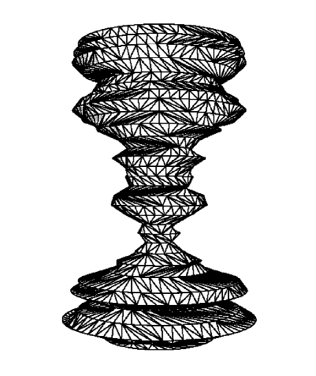
Figure 1: A typical discrete history of pure Lorentzian gravity with volume N=1024.

We managed in [1] to further trace the difference between the two quantum theories to the presence or absence of so-called baby universes. These are outgrowths of the two-geometry giving it the structure of branchings-over-branchings, which are known to dominate the typical geometry contributing to the Euclidean state sum. On the other hand, in the Lorentzian state sum, one can suppress the formation of such branchings with respect to the preferred spatial slicing (which is not present in the Euclidean picture, where no directions are distinguished). There is also a physical motivation for suppressing the generation of baby universes, since the associated (discrete) geometries can usually not be embedded isometrically in a smooth Lorentzian space-time. If nevertheless one did decide to generalize the evolution rules of the Lorentzian model to allow for such branchings (and keep only a weaker notion of causality, c.f. [1]), one would rederive the usual Euclidean Liouville results. In what follows, when talking about ‘the Lorentzian model’, we will mean the unmodified model without branching baby universes, i.e. the model of 2d quantum gravity that does not lie in the same universality class as Liouville gravity. We also would like to point out that from the point of view of a canonical quantization the Lorentzian model is much more natural. The inclusion of topology changes of space into a canonical scheme would require a so-called third quantization of geometry.

In Liouville gravity, matter couples strongly to geometry, perhaps even too strongly in the sense that the combined system becomes inconsistent when the central charge of the (conformal) matter exceeds one. Arguments have been presented which link the strong deformation of geometry to the creation of baby universes [9]. It is therefore conceivable that the Lorentzian model of gravity – where baby universes are absent – has a weaker and less pathological coupling to matter.

In order to understand the behaviour of the combined gravity-matter system, we are considering here the coupling of the gravitational model of reference [1] to an Ising model of spin-$\frac{1}{2}$, with nearest-neighbour interaction $\sum_{<ij>}\sigma_{i}\sigma_{j}$ between its spins $\sigma_{i}\!=\!\pm 1$. In [1] we made a careful analysis of the implications of the Lorentzian signature for the sum over space-time metrics. The most straightforward way of obtaining the continuum limit consisted in performing the calculations in the discretized model with purely imaginary coupling (corresponding to Euclidean signature) and only afterwards ‘rotating back’ to the Lorentzian sector. Moreover, it turned out that certain simple properties, like the fractal dimension of space-time, were independent of the analytic continuation.

We will apply the same philosophy in the present context by analyzing the Ising model coupled to 2d gravity with coupling constants corresponding to the Euclidean signature sector. Nevertheless we will continue to talk about ‘Lorentzian’ gravity coupled to matter, because the choice of two-dimensional Euclidean geometries contributing to the path integral is dictated by the requirement that after the rotation to Lorentzian signature they should be causal and non-singular. The ‘matter observables’ we will consider are the critical exponents for the Ising model, characterizing the underlying $c\!=\!1/2$ fermionic continuum model coupled to gravity, which are not expected to change under the rotation to Lorentzian signature. In order to determine the universality class of the interaction between matter and gravity it is therefore convenient to work entirely within the Euclidean sector of our Lorentzian gravity model.

For fixed regular two-dimensional lattices, and in the absence of an external magnetic field, the Ising model can be solved exactly in a variety of ways (see, for example, [3, 4, 5]). The partition function (for the square lattice) was found by Onsager. Its critical behaviour is characterized by a logarithmic singularity of the specific heat and the critical exponents near the Curie temperature, $\alpha\!=\!0$, $\beta\!=\!0.125$, and $\gamma\!=\!1.75$, for the specific heat, the spontaneous magnetization and the susceptibility respectively.

For the case of the usual Euclidean 2d gravity, described by an ensemble of planar random surfaces, coupling to Ising spins was first considered in [6], where an exact solution was obtained with the help of matrix model methods. It could be shown that in the presence of gravity, the matter behaviour is ‘softened’ to a third-order phase transition, characterized by critical exponents $\alpha\!=\!-1$, $\beta\!=\!0.5$, and $\gamma\!=\!2$ [7]. On the other hand, the geometry is ‘roughened’, as exemplified by the increase from $-1/2$ (pure 2d Liouville gravity) to $-1/3$ of the entropy exponent $\gamma_{string}$ for baby universes on manifolds of spherical topology.

It is not entirely straightforward to apply the methods used to obtain these exact solutions to the Lorentzian gravity model. For example, one can write down an expression for the transfer matrix generalizing that of the Onsager solution by imposing a length cutoff $l_{0}$ on the length of spatial slices. However, a major stumbling block to understanding the behaviour of its eigenvalues as $l_{0}\rightarrow\infty$ is the fact that as a consequence of the gravitational degrees of freedom, transitions between spatial slices of different length are allowed. This makes the use of Fourier transforms problematic, which are an essential ingredient of this and other algebraic solution schemes. Moreover, the Hilbert space dimension for the discrete, finite model is given by $\sum_{l=1}^{l_{0}}2^{l}$, which grows rapidly with $l_{0}$.

In the absence of an analytic exact solution, one way to try to extract information about the matter-coupled model is by performing a series expansion of the partition function $Z$ at high or low temperature, or of suitable derivatives of $Z$. For flat, regular lattice geometries, these have been studied extensively since the early days of the Ising model. It is well-known that the high-$T$ expansion, in particular, that of the magnetic susceptibility $\chi$ at zero field is well-suited for obtaining information about the critical behaviour of the theory. We will show that the same is true for the coupled gravity-Ising model, after taking into account some peculiarities to do with the fact that we have an ensemble of fluctuating geometries instead of a fixed lattice. In the limit of large lattice size $N$, there is a well-defined expansion in terms of $u:=\tanh\beta$, where the coupling $\beta$ is proportional to the inverse temperature, whose coefficients can be determined by diagrammatic techniques. Given a plausible ansatz for the singularity structure of the thermodynamic functions, one can then extract estimates for the critical point and critical exponents from the first few terms of such an expansion. These results are corroborated by performing a Monte Carlo simulation of Lorentzian gravity coupled to the Ising model. Apart from being in good agreement with the high-$T$ expansion, the simulations also allow us to measure the quantum geometrical properties of the model.

2 The high-$T$ expansion

Recall the usual high-$T$ expansion of the Ising model on a fixed lattice of volume $N$, with partition function

$$Z(\beta,N)=\sum_{\{\sigma_{i}=\pm 1\}}\mbox{e}^{\beta\sum\limits_{<ij>}\sigma_{i}\sigma_{j}+H\sum\limits_{i}\sigma_{i}},\hskip 56.9055pt\beta=\frac{J}{kT},$$ (2)

where the sum is taken over all possible spin configurations, and $J>0$ denotes the ferromagnetic Ising coupling. We will only consider the case of vanishing magnetic field, $H\!=\!0$. The Ising spins are located at the lattice vertices, labelled by $i,j\in 1\ldots v$. A convenient expansion parameter at high temperature is $u:=\tanh\beta$, which we can use to re-express

$$\mbox{e}^{\beta\sigma_{i}\sigma_{j}}=(1+u\,\sigma_{i}\sigma_{j})\cosh\beta.$$ (3)

Substituting (3) into (2), the partition function becomes

$$Z(\beta,N) = (\cosh\beta)^{s}\sum_{\{\sigma_{i}\}}\Bigl{[}1+u\sum_{<ij>}\sigma_{i}\sigma_{j}+u^{2}\sum_{<ij>}\sum_{<kl>}(\sigma_{i}\sigma_{j})(\sigma_{k}\sigma_{l})+\ldots\Bigr{]}$$ (4)

$$=: 2^{v}(\cosh\beta)^{s}(1+\sum_{n\geq 1}\Omega_{n}u^{n}),$$ (5)

with $v$ denoting the number of vertices and $s$ the number of nearest-neighbour pairs (i.e. the number of lattice links). Note that the terms $\sim u^{n}$ in eq. (4) are only non-vanishing if every $\sigma_{i}$ in $\sigma_{i_{1}}\sigma_{i_{2}}\ldots\sigma_{i_{n}}$ appears an even number of times. Representing spin pairs $(\sigma_{i}\sigma_{j})$ by drawing a link between $\sigma_{i}$ and $\sigma_{j}$ on the lattice, this is equivalent to the following statement: non-vanishing contributions to $\Omega_{n}$ in eq. (5) correspond to figures of lattice links which are closed polygons, with an even number of links meeting at each vertex. The coefficient $\Omega_{n}$ simply counts the number of such figures at order $n$ that can be put down on a given lattice, and will depend on the lattice geometry (triangular, square, etc.). It is a polynomial in the variable $N$.

Because of the extensive nature of the free energy $F(N)\!=\!-kT\ln Z(N)$, we must have that $(1+\sum\Omega_{n}u^{n})\sim\mbox{e}^{N(\ldots)}$ in the thermodynamic limit $N\to\infty$, and we can therefore write for the partition function per unit volume

$$\ln Z(\beta):=\frac{1}{N}\ln Z(\beta,N)=\frac{s}{N}\,\cosh\beta+\frac{v}{N}\,\ln 2+\sum_{n\geq 1}\omega_{n}^{(0)}u^{n},$$ (6)

where $\omega_{n}^{(0)}$ is obtained by taking the term linear in $N$ in $\Omega_{n}$ and setting $N\!=\!1$. Note that both connected and disconnected graphs contribute to $\omega_{n}^{(0)}$. A similar relation can be obtained for the magnetic susceptibility at zero field, $\chi(N)=kT\frac{\partial^{2}}{\partial H^{2}}\ln Z(N)|_{H=0}$. At high temperature, the susceptibility per unit volume can be expressed as

$$\chi=kT\ (1+\sum_{n\geq 1}\omega_{n}^{(2)}u^{n}).$$ (7)

The coefficients $\omega_{n}^{(2)}$ are the exact analogues of $\omega_{n}^{(0)}$ in eq. (6), where the counting now refers to polygon graphs with two odd vertices (vertices with an odd number of incoming links), and all other vertices even (c.f. [8], but beware of the difference in notation for the number of vertices).

Since we are primarily interested in the bulk behaviour of the gravity-matter system, we will in the following for simplicity choose the boundary conditions to be periodic. That is, we will identify the top and bottom spatial slices of the cylindrical histories introduced in [1]. Clearly this is not going to affect the local properties of the model. As above, we will denote the discrete volume, i.e. the number of triangles of a given two-dimensional geometry (with torus topology), by $N$. It follows immediately that such a geometry contains $N$ time-like links, $N/2$ space-like links, $N/2$ vertices and $3N/2$ nearest-neighbour pairs.

In quantum gravity the volume $N$ becomes a dynamical variable. For fixed topology, the only coupling constant appearing in the action of pure 2d quantum gravity is the cosmological constant, multiplying the volume term. The partition function of the Ising model coupled to 2d Lorentzian quantum gravity is given by

$$G(\lambda,t,\beta)=\sum_{T\in{\cal T}_{t}}e^{-\lambda N_{T}}Z_{T}(\beta)=\sum_{T\in{\cal T}_{t}}e^{-\lambda N_{T}}\sum_{\{\sigma_{i}(T)\}}\mbox{e}^{\beta\sum\limits_{\left\langle ij\right\rangle\in T}\sigma_{i}\sigma_{j}},$$ (8)

where the sum is taken over all triangulations $T$ with the topology of a torus and $t$ time-slices, $N_{T}$ is the number of triangles in $T$, and $Z_{T}(\beta)$ the Ising partition function (2) defined on $T$. Fortunately, the summation over volumes in eq. (8) does not lead to additional complications in the analysis of the thermodynamic properties of the spin system, since the state sums for fixed and fluctuating volume are simply related by a Laplace transformation. Rewrite relation (8) as

$$G(\lambda,t,\beta)=\sum_{N}e^{-\lambda N}\tilde{Z}(\beta,N,t):=\sum_{N}e^{-\lambda N}\sum_{T\in{\cal T}_{N,t}}Z_{T}(\beta),$$ (9)

where ${\cal T}_{N,t}$ denotes the toroidal triangulations of volume $N$ and length $t$ in the time direction. Analogous to eq. (6), we expect the matter part $f(\beta)$ of the free energy density in the gravitational ensemble to behave in the thermodynamic limit ($N\to\infty$ and $t\propto\sqrt{N}$) like

$$\tilde{Z}(\beta,N,t)\to e^{(\lambda_{c}-\beta f(\beta))N+o(N)}.$$ (10)

(For simplicity, we have set the ferromagnetic coupling to $J\!=\!1$.) We can now reexpress eq. (9) as

$$G(\lambda,t,\beta)=\sum_{N}e^{(\lambda_{c}(\beta)-\lambda)N+o(N)},~{}~{}~{}~{}\lambda_{c}(\beta)=\lambda_{c}-\beta f(\beta),$$ (11)

where $\lambda_{c}\equiv\lambda_{c}(\beta\!=\!0)\!=\!\ln 2$ is the critical cosmological constant of pure gravity, which was determined in [1]. Interesting limiting cases are $\beta\to 0$ where $-\beta f(\beta)=\frac{1}{2}\ln 2$, reflecting the factor $2^{v}$ in eq. (4) (each spin has two states), and the strong coupling region $\beta\to\infty$ where $-\beta f(\beta)\to 3\beta/2$ (only the ground state of all spins aligned contributes to the state sum (2)). The term proportional to the pure gravity cosmological constant $\lambda_{c}$ appearing together with the free energy in (10) has its origin in the sum over all triangulations,

$$\sum_{T\in{\cal T}_{N,t}}1=e^{\lambda_{c}N+o(N)}.$$ (12)

A calculation of $\tilde{Z}(\beta,N,t)$ not only determines the thermodynamic properties of the spin system in the presence of gravity, but at the same time describes gravitational aspects of the coupled system, for example, the critical cosmological constant $\lambda_{c}(\beta)$. Conversely, knowledge of $\lambda_{c}(\beta)$ determines the spin partition function in the infinite volume limit. – The analogue of the high-$T$ expansion (5) in the presence of gravity is given by

$$\tilde{Z}(\beta,N,t)=(\cosh\beta)^{\frac{3N}{2}}\ 2^{\frac{N}{2}}\sum_{T\in{\cal T}_{N,t}}(1+\sum_{n\geq 1}\tilde{\Omega}_{n}(T)u^{n}).$$ (13)

We may reexpress the critical cosmological constant of the combined system as

$$\lambda_{c}(\beta)=\lambda_{c}+\frac{3}{2}\ln\cosh\beta+\frac{1}{2}\ln 2+\tilde{f}(u),$$ (14)

where $\tilde{f}(u)$ is defined in the thermodynamic limit by

$$\frac{\sum\limits_{T\in{\cal T}_{N,t}}(1+\sum\limits_{n\geq 1}\tilde{\Omega}_{n}(T)u^{n})}{\sum\limits_{T\in{\cal T}_{N,t}}1}=e^{N\tilde{f}(u)}.$$ (15)

The coefficients $\tilde{\Omega}$ of the power series now depend on the triangulation $T$. When counting diagrams of a given type and order $n$, we must keep in mind that the vertex neighbourhoods do not look all the same, as they do in the case of a regular lattice, but that the distribution of coordination numbers (numbers of links meeting at a vertex) is subject to a probability distribution. The coefficients in the high-$T$ expansion therefore count the average occurrence of a certain diagram type in the ensemble of triangulations of a fixed volume $N$, for large $N$.

Starting to evaluate the series in (13) order by order, one immediately notices a qualitative difference from the regular case. If we had considered a regular triangular lattice (coordination number 6), the first non-trivial contribution to the counting of even diagrams would have appeared at $n\!=\!3$, where one obtains $\Omega_{3}(N)\!=\!N$, coming from closed triangle graphs. However, when looking at all two-dimensional random lattices contributing to the sum over geometries in the gravity case, there are geometries which have one or several ‘pinches’. A pinch is a spatial slice of minimal length $l\!=\!1$, which consists of a single link and a single vertex (see Fig. 2). Pinches occur even if the total volume of the two-geometry is kept fixed, since in the presence of gravity the length of spatial slices is a fluctuating dynamical variable.

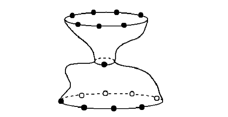
Figure 2: A two-dimensional geometry with a ‘pinch’ of length 1.

For the gravitationally coupled Ising model, the lowest-order contribution to the power series in $u$ in (13) occurs therefore already at order $n\!=\!1$. Clearly, such pinching contributions will be present at all orders, in both connected and disconnected diagrams, on top of the ordinary ‘bulk’ contributions, coming from diagrams which do not wind around the spatial direction of the torus in a non-trivial way. The former have no analogue on regular lattices.

Fortunately, it turns out that the pinch contributions are irrelevant, in the sense that they contribute at a lower order of $N$, whereas the bulk contributions in $\tilde{\Omega}_{n}$ go like $N^{k}$, $k\geq 1$. This can be seen most easily by considering the Laplace-transformed partition function. Let us begin by evaluating the zeroth-order term of eq. (13),

$$G(\tilde{\lambda},t)=\sum_{N}\mbox{e}^{-\tilde{\lambda}N}\sum_{T\in{\cal T}_{N,t}}1:=\sum_{N}\mbox{e}^{-\lambda N}(\cosh\beta)^{\frac{3N}{2}}\ 2^{\frac{N}{2}}\sum_{T\in{\cal T}_{N,t}}1,$$ (16)

where for notational brevity we have defined an ‘effective cosmological constant’ $\tilde{\lambda}\!=\!\lambda-\frac{3}{2}\ln\cosh\beta-\frac{1}{2}\ln 2$, in accordance with eq. (14). The left-hand side of (16) can be computed as

$$G(\tilde{\lambda},t)=\oint\frac{dx}{2\pi ix}\;G(x,y=\frac{1}{x};\mbox{e}^{-\tilde{\lambda}};t),$$ (17)

given the explicit form of the propagator derived in ref. [1], to which we also refer for details of notation. The term proportional to $u^{1}$ in the Laplace transform of (13) is

$$\sim u^{1}:\hskip 22.76228pt\sum_{N}\mbox{e}^{-\tilde{\lambda}N}\sum_{T\in{\cal T}_{N,t}^{l=1}}1=G(\tilde{\lambda},t)\,\tilde{\Omega}_{1}^{\rm norm}(\tilde{\lambda}),$$ (18)

where the second summation is over triangulations with a single ‘pinch’ of spatial length $l\!=\!1$. To arrive at the last expression on the right-hand side, the factor $G(\tilde{\lambda},t)$ has been pulled out. In terms of quantities derived in [1], the normalized coefficient $\tilde{\Omega}_{1}^{\rm norm}$ is most easily computed as

$$\tilde{\Omega}_{1}^{\rm norm}(\tilde{\lambda})=\frac{\sum\limits_{{\tilde{t}}=1}^{t-1}G_{\tilde{\lambda}}(x,l\!=\!1;\tilde{t})G_{\tilde{\lambda}}(l\!=\!1,y;t-\tilde{t})}{G_{\tilde{\lambda}}(x,y;t)}\Big{|}_{x=y=0}.$$ (19)

We are interested in the behaviour of this expression in the thermodynamic limit, which is tantamount to letting the cosmological constant approach its critical value, $\tilde{\lambda}\to\tilde{\lambda}_{c}$. In this limit, (19) yields simply a constant, $\tilde{\Omega}_{1}^{\rm norm}\buildrel a\rightarrow 0\over{\longrightarrow}2$. This is a general feature of configurations with one or several pinches. For example, generalizing to geometries with a single pinch of length $l$ gives a coefficient $2l$ in the large-volume limit. As an example of a more complicated configuration, the normalized coefficient for histories with one pinch of length $l_{1}$ and a second one of length $l_{2}$ becomes in this limit

$$\sim u^{l_{1}+l_{2}}:\hskip 17.07182pt\buildrel a\rightarrow 0\over{\longrightarrow}\,3\sum_{k=0}^{{\rm min}(l_{1},l_{2})-1}(-1)^{k}\frac{(l_{1}+l_{2}-k-1)!}{(l_{1}-k-1)!(l_{2}-k-1)!k!}.$$ (20)

By contrast, let us now calculate the first bulk contribution, which occurs at order $u^{3}$. The contribution to $\tilde{\Omega}_{3}$ is simply $N$, from counting the number of triangle graphs in the 2d geometry. Taking the Laplace transform, we obtain

$$\sum_{N}\mbox{e}^{-\tilde{\lambda}N}N\equiv-\frac{\partial}{\partial\tilde{\lambda}}G(\tilde{\lambda},t)\equiv\left\langle N\right\rangle\,G(\tilde{\lambda},t).$$ (21)

Evaluating the expectation value of $N$ in the continuum limit, one finds

$$\left\langle N\right\rangle\ = -G(\tilde{\lambda},t)^{-1}\,\frac{\partial}{\partial\tilde{\lambda}}G(\tilde{\lambda},t)$$ (22)

$$\buildrel a\rightarrow 0\over{\longrightarrow} -\frac{4\,(1-\mbox{e}^{-2T\sqrt{\Lambda}}-T\sqrt{\Lambda}(1-\mbox{e}^{-2T\sqrt{\Lambda}}))}{a^{2}\Lambda(1-\mbox{e}^{-2T\sqrt{\Lambda}})}\,\buildrel T\;{\rm large}\over{\longrightarrow}\,\frac{4T}{a^{2}\sqrt{\Lambda}}.$$ (23)

(We are using the notation of [1], with $T$ and $\Lambda$ the continuum length of the two-geometry in ‘time’-direction and the renormalized cosmological constant.) This diverges exactly the way one would expect from a volume term. It reiterates the conclusion of [1] that all macroscopic metric variables scale canonically in the Lorentzian gravity model.

We conclude that in the thermodynamic limit, pinching terms will be suppressed since their number is proportional to $N^{0}$, whereas the (connected) bulk diagrams behave like $\sim N^{1}$. For large $N$, the pinch contributions must therefore factorize according to

$$(1+\sum_{n\geq 1}\tilde{\Omega}_{n}(T)u^{n})=(1+N^{0}\sum_{m\geq 1}p_{m}(T)u^{m})\,(1+N\,\sum_{n\geq 1}\tilde{\omega}_{n}(T)u^{n}+O(N^{2})).$$ (24)

Taking the logarithm, we see that the sum $(1+\sum p_{m}(T)u^{m})\sim N^{0}$ will only contribute a constant term to the free energy, which does not affect the universal behaviour of the model. We will make no attempt to calculate it explicitly. Similar considerations apply to the high-$T$ expansion of the magnetic susceptibility in the presence of gravity. The pinch contributions factorize, and we will only need to compute the multiplicity $\tilde{\omega}_{n}^{(2)}$ of bulk polygon graphs with two odd vertices per triangle in

$$\chi\sim(1+\sum_{n\geq 1}\tilde{\omega}_{n}^{(2)}u^{n}).$$ (25)

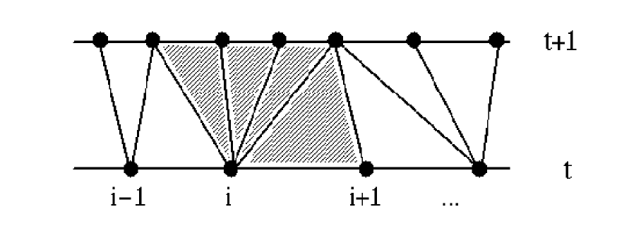
Figure 3: The triangles contributing to the weight at the vertex $i$.

Our next step will be to derive the probability distribution of the coordination numbers in the Lorentzian gravity model, in the thermodynamic limit as the cosmological constant $\lambda\to\lambda_{c}\!=\!\ln 2$. Recall that when generating an interpolating space-time between an initial and a final spatial geometry, the geometry of each space-time ‘sandwich’ with $\Delta t\!=\!1$ is independent of the previous one in the sense that there are no local constraints on how the numbers $k_{i}\geq 1$ of time-like future-pointing links can be chosen at each vertex $i$ [1]. Having reached a spatial slice at time $t$, we can generate the space-time between $t$ and $t\!+\!1$ proceeding from ‘left to right’. To each vertex $i$ at time $t$ we associate $k_{i}$ time-like links (ending at vertices of the subsequent spatial slice at $t+1$) and the space-like link to the right of the vertex. There are therefore exactly $k_{i}$ triangles associated with the vertex $i$, contributing with a weight factor $e^{-k\lambda}$ to the action, as illustrated in Fig. 3. Since the assignment of the order $k_{i}$ of outgoing time-like links to the vertex is completely independent of the $k$-assignments of other vertices, the probability distribution for $k$ outgoing future-directed links is given by

$$p_{\lambda}(k)=e^{-k\lambda}(e^{\lambda}-1).$$ (26)

Strictly speaking, the argument leading to eq. (26) is only correct in the continuum limit in which ‘extreme pinching’ to vanishing spatial length $l\!=\!0$ does not occur (for off-critical $\lambda$, relation (26) must be modified to account for the fact that moves changing the torus topology are forbidden). Fortunately this is the only case we are interested in, and the final probability distribution is therefore obtained by setting $\mbox{e}^{-\lambda}=1/2$ in (26), yielding

$$p(k)\equiv p_{\lambda_{c}}(k)=\frac{1}{2^{k}}.$$ (27)

For reasons of symmetry, the distribution of incoming time-like links at $i$ (originating at the slice at $t\!-\!1$) is of course identical. Given relation (27), we can now compute the probability distribution $\tilde{p}(j)$ of the vertex order, i.e. of the total number $j$ of links meeting at a vertex (incoming and outgoing time-like and space-like links),

$$\tilde{p}(j)=\frac{j\!-\!3}{2^{j-2}},\hskip 28.45274ptj\geq 4.$$ (28)

With the distribution (27) in hand, we can now embark on the actual counting of diagrams contributing to the susceptibility coefficients $\tilde{\omega}_{n}^{(2)}$ in (25). We will only quote the results up to order $n\!=\!5$. Further details of the counting procedure will appear elsewhere. The average numbers of diagrams per triangle (i.e. per unit volume) are listed in the table below.

$n$	open	closed	disconnected	total
1	$\frac{3}{2}$	0	0	$\frac{3}{2}$
2	$8\frac{1}{2}$	0	0	$8\frac{1}{2}$
3	$43\frac{1}{2}$	0	0	$43\frac{1}{2}$
4	$214\frac{5}{6}$	14	$-17$	$211\frac{5}{6}$
5	$1038\frac{1}{6}$	$134\frac{5}{18}$	$-174\frac{17}{18}$	$997\frac{1}{2}$

Open graphs are connected graphs without any self-intersections. Closed graphs are connected graphs which are not open. The disconnected graphs consist of two or more components and contribute with a minus sign.

In order to double-check our results at order 4 and 5, where the counting becomes slightly involved, we have performed a numerical check on the coefficients $\tilde{\omega}_{n}^{(2)}$ listed above. This was done by computer-generating histories of length $\Delta t\sim 100$, with an initial spatial slice of length $\Delta l\!=\!200$, and counting diagrams of a given type. The results are given in the table below and in very good agreement with the exact calculation. They are based on a total of $\sim 3\times 10^{5}$ vertices at order 4 and $\sim 9\times 10^{5}$ vertices at order 5. We have not listed the counting of disconnected graphs separately, since it follows closely the counting of closed connected graphs.

$n$	open	closed
4	$214.642\pm 0.179$	$13.996\pm 0.007$
5	$1037.770\pm 0.751$	$134.197\pm 0.098$

2.1 Evaluation of results

In order to evaluate the results from the high-$T$ expansion, we assume a simple behaviour of the susceptibility of the form

$$\chi(u)\sim A\,\Bigl{(}1-\frac{u}{u_{c}}\Bigr{)}^{-\gamma}+B$$ (29)

near the critical point $u_{c}$, with analytic functions $A$ and $B$. Using the ratio method (see, for example, [11]), we have fitted the susceptibility coefficients to

$$r_{n}=\frac{\tilde{\omega}_{n}^{(2)}}{\tilde{\omega}_{n-1}^{(2)}}=\frac{1}{u_{c}}\Bigl{(}1+\frac{\gamma\!-\!1}{n}\Bigr{)}.$$ (30)

Plotting the ratios $r_{n}$ linearly against $1/n$ for $n\in 1\ldots n_{\rm max}$, we have extracted the following estimates for the critical point $u_{c}$ and the critical susceptibility exponent $\gamma$:

$n_{\rm max}$	critical point	critical exponent
3	$u_{c}=0.2488$	$\gamma=1.820$
4	$u_{c}=0.2462$	$\gamma=1.789$
5	$u_{c}=0.2458$	$\gamma=1.783$

The estimates for the critical exponent should be compared to the exact values for $\gamma$ for the Ising model on a fixed, regular lattice and on dynamically triangulated lattices (Ising spins coupled to Euclidean quantum gravity), which are $\gamma^{\rm reg}\!=\!1.75$ and $\gamma^{\rm dt}\!=\!2$ respectively. The data from the high-$T$ expansion clearly favour $\gamma=1.75$ in our model. Indeed, the estimates for $\gamma$ are remarkably close to this value, given that we are working only up to order 5 in the expansion parameter $u\!=\!\tanh\beta$. The conclusion that the critical exponents of the Ising model coupled to Lorentzian quantum gravity coincide with those found on regular lattices is also supported by the Monte Carlo simulations we have performed.

However, before turning to a detailed description of the simulations we would like to illustrate how well the high-$T$ expansion works even at this rather low order. We will compare the $\beta$–dependent cosmological constant $\lambda_{c}(\beta)$ defined in eq. (14), which can be measured directly in the Monte Carlo simulation, with the same quantity obtained from the high-$T$ expansion. Recall that in the thermodynamic limit $\lambda_{c}(\beta)$ is essentially given by the spin free energy, eq. (11), which can be computed in the small-$\beta$ expansion. We have determined the density $\tilde{f}(u)$, defined in eq. (15), by counting closed polygon graphs in the high-$T$ expansion up to order 6. Inserting this into formula (14) leads to

$$\lambda_{c}^{\rm high-T}(\beta)=\lambda_{c}+\frac{1}{2}\ln 2+\frac{3}{2}\ln\cosh\beta+u^{3}+\frac{5}{3}u^{4}+\frac{35}{9}u^{5}+\frac{263}{27}u^{6}.$$ (31)

In Fig. 4 we show the data points for $\lambda_{c}(\beta)-3\beta/2$ as measured by the Monte Carlo simulation. Since $\lambda_{c}\!=\!\ln 2$ in pure gravity, the data should approach $\frac{3}{2}\ln 2$ for $\beta\to 0$ and $\lambda_{c}\!=\!\ln 2$ for $\beta\to\infty$, both of which are well satisfied. In order to quantify the effect of the $u$-expansion, we have plotted both the zeroth-order expression $F_{1}(\beta)=\lambda_{c}+\frac{1}{2}\ln 2+\frac{3}{2}\ln\cosh\beta-\frac{3}{2}\beta$, and the improved sixth-order expression $F_{2}(\beta)=\lambda^{\rm high-T}_{c}(\beta)-\frac{3}{2}\beta$. The latter agrees well with the measured Monte Carlo values right up to the neighbourhood of the critical Ising coupling $\beta_{c}$. At the critical point $\beta_{c}$ the measured function $\lambda_{c}(\beta)$ exhibits a cusp. This reflects the singular part contained in $\lambda_{c}(\beta)$ which of course cannot be captured by simply plotting the analytic function (14).

Figure 4: The critical cosmological constant as a function of the Ising coupling $\beta$, as measured by Monte Carlo simulations ($t\!=\!32$, $N\!=\!2048$), and compared to the corresponding high-$T$ expansions $F_{1}(\beta)$ and $F_{2}(\beta)$ at order 0 and order 6.

3 The Monte Carlo simulation

Monte Carlo simulations have been used successfully in the study of Euclidean 2d quantum gravity. The formalism known as ‘dynamical triangulations’ provides a regularization of the functional integral well-suited for such simulations, allowing in addition for a straightforward matter coupling of Gaussian fields as well as of spin degrees of freedom. Extensive computer simulations of the combined gravity-matter systems have been performed, leading to results in perfect agreement with exact results derived from Liouville theory and matrix model calculations.

The Lorentzian model resembles the dynamically triangulated model in that its dynamics is associated with the fluctuating connectivity of the triangulations contributing to the path integral. This allows us to take over many of the techniques from the computer simulations of the dynamically triangulated models. We must specify the update of both the geometry and the matter fields, the latter being standard: for a given triangulation we update the spin configurations by the same spin cluster algorithms used for dynamical triangulations. This presents no problems since our configurations form a subset of the full set of dynamical triangulations used in Euclidean quantum gravity (on the torus). During the update of geometry, we want to keep the number of time-slices fixed while allowing any space-like fluctuations compatible with the model. A local change of geometry or ‘move’ which is clearly ergodic (i.e. can generate any of the allowed configurations when applied successively) is shown in Fig. 5. It consists in deleting the two triangles adjacent to a given space-like link (if the resulting configuration is allowed). Its inverse is a ‘split’ of a given vertex and two neighbouring time-like links into two, thereby creating a new space-like link, as well as two new triangles. This is a special case of the so-called ‘grand canonical move’ sometimes used in dynamical triangulation simulations [12, 13, 2], and does not preserve the total volume of space-time.

Figure 5: The move used in the Monte Carlo updating of the geometry.

Detailed balance equations for the move can be derived from standard considerations [2]. Let $N_{V}$ denote the number of vertices ($N_{V}=N/2$, where $N$ is the number of triangles), and $v$ a specific vertex. For pure Lorentzian gravity without matter, the equation for detailed balance reads

$$P(N_{V})\frac{P(N_{V}\!\to\!N_{V}\!+\!1)}{N_{V}k_{in}k_{out}}=P(N_{V}\!+\!1)P(N_{V}\!+\!1\!\to\!N_{V}),$$ (32)

where $P(N_{V})=\frac{e^{-2\lambda N_{V}}}{N_{V}!}$ is the probability distribution for labelled triangulations, and $k_{in}$ and $k_{out}$ count the incoming and outgoing time-like links at $v$ (see Fig. 5). We are still free to choose $P(N_{V}\!\to\!N_{V}\!+\!1)$ and $P(N_{V}\!+\!1\!\to\!N_{V})$ such that condition (32) is satisfied. Once a transition probability $P(N_{V}\!+\!1\!\to\!N_{V})$, say, has been chosen, it will be tested during the simulation against the uniform probability distribution between 0 and 1 as follows. Choose a random number $r\in]0,1]$. Then, if the move is allowed (i.e. if the resulting triangulation belongs to the allowed class of configurations) it is accepted if $P(N_{V}\!+\!1\!\to\!N_{V})>r$. If it is not allowed, one proceeds to the next move.

It is straightforward to generalize the updating of geometry to include Ising spins. The spin Hamiltonian is included in $P(N_{V})$, which now becomes a function of both $N_{V}$ and the spin configurations. When inserting a vertex $v$, one has to specify at the same time a spin associated with $v$. The choice of spin up or down is made with probability 1/2, and the final result tested as in the case of the pure geometry update.

We have performed the computer simulation for surfaces with toroidal topology and for system sizes of $N$=2048, 4050, 8192, 16200 and 32768 triangles, and with a number $t$=32, 45, 64, 90 and 128 of time-slices respectively. Since the moves are not volume-preserving, fixing the system size to $N$ is implemented as follows: we allow the volume to fluctuate within a certain, not too wide range, and collect for every sweep the first configuration with volume $N$. The volume fluctuations are controlled by adding a term $\delta\lambda\,(\Delta N)^{2}$ to the action, where $\Delta N$ is the deviation of the volume from its desired value $N$. This term does not affect the ensemble of configurations collected, since for all of them $\Delta N\!=\!0$. We find that $\left\langle\Delta N\right\rangle^{-1}\sim\sqrt{\delta\lambda}$. Finally, one checks that the results obtained do not depend on the chosen, allowed range of volume fluctuations. A sweep is a set of approximately $N_{V}$ accepted moves. For each $\beta$-value used in the multi-histogramming analysis we perform $1.25\times 10^{6}$ sweeps ($0.75-1.00\times 10^{6}$ for $N=32768$). Measurements are made every $5$ sweeps and errors are computed by data binning.

3.1 Numerical results for the spin system

The determination of the critical properties of the Ising spin system coupled to Lorentzian gravity proceeds in two steps (see [14] for a recent, more complete discussion in the context of 2d Euclidean quantum gravity). We first locate the critical $\beta$-value where the system undergoes a transition from a magnetized (at large $\beta$) to an unmagnetized phase. Next, we perform simulations in the neighbourhood of the critical value $\beta_{c}$ and use finite-size scaling to determine the critical exponents. Finite-size scaling is also very useful for determining the location of the critical coupling $\beta_{c}$ itself, since a number of standard observables show a characteristic behaviour for $\beta$ close to $\beta_{c}$. The following are some of the observables we have used, together with their expected finite-size behaviour (see [14] for a full list):

$$\chi=N(\left\langle m^{2}\right\rangle-\left\langle|m|\right\rangle^{2})\sim N^{\gamma/\nu d_{H}}~{}~{}~{}~{}~{}~{}~{}~{}~{}~{}~{}~{}{\rm(susceptibility)}$$ (33)

$$D_{\ln|m|}=N\Big{(}\left\langle e\right\rangle-\frac{\left\langle e|m|\right\rangle}{\left\langle|m|\right\rangle}\Big{)}\sim N^{1/\nu d_{H}}~{}~{}~{}~{}~{}~{}(D_{\ln|m|}\equiv\frac{d\ln|m|}{d\beta})$$ (34)

$$D_{\ln m^{2}}=N\Big{(}\left\langle e\right\rangle-\frac{\left\langle em^{2}\right\rangle}{\left\langle m^{2}\right\rangle}\Big{)}\sim N^{1/\nu d_{H}}~{}~{}~{}~{}~{}(D_{\ln m^{2}}\equiv\frac{d\ln m^{2}}{d\beta}),$$ (35)

where $\gamma$ and $\nu$ are the critical exponents of the susceptibility and of the divergent spin-spin correlation length, and $d_{H}$ is the Hausdorff or fractal dimension of space-time. For a flat space-time (where of course $d_{H}\!=\!d\!=\!2$), we have $\nu d$ = 2, whereas for the Ising model coupled to Euclidean quantum gravity $\nu d_{H}$ = 3 (and $d_{H}\approx 4$). The internal energy density $e$ and the magnetization $m$ of the spin system are defined by

$$e=\frac{-1}{NZ_{N}(\beta)}\frac{dZ_{N}(\beta)}{d\beta},~{}~{}~{}~{}m=\frac{1}{NZ_{N}(\beta,H)}\frac{dZ_{N}(\beta,H)}{dH}\;\Big{|}_{H=0}.$$ (36)

In order to find the critical point $\beta_{c}$, we can use the fact that the pseudo-critical coupling $\beta_{c}(N)$ at volume $N$ is expected to behave like

$$\beta_{c}(N)\sim\beta_{c}+\frac{c}{N^{1/\nu d_{H}}}$$ (37)

close to $\beta_{c}\!=\!\beta_{c}(N\!=\!\infty)$, with $c$ a constant. The observables (33)-(35) all have well-defined peaks which we used for a precise location of $\beta_{c}(N)$, with the help of multi-histogram techniques. Eq. (37) can now be used to extract $\beta_{c}$ and $1/\nu d_{H}$. However, it is advantageous to determine first $1/\nu d_{H}$ from the peak values of (34) and (35), and then substitute this value into (37), thus reducing the number of free parameters in the fit. Afterwards, one can check that consistent values for $1/\nu d_{H}$ are obtained from the observables (34) and (35) at $\beta_{c}$, using multi-histogramming. In our simulations, $1/\nu d_{H}$ extracted from the peaks was so close to the Onsager value 1/2 that we did not hesitate to use $1/\nu d_{H}\!=\!1/2$ in (37). Leaving it as a free parameter one obtains consistent results, but the error in $\beta_{c}$ becomes larger. Finally, we have determined $\gamma/\nu d_{H}$ from (33), both from the peak values and at $\beta_{c}$ (and again using multi-histogramming).

In the table below we have listed the $\beta_{c}$-values extracted from measuring $D_{\ln|m|}$ and $D_{\ln m^{2}}$, and assuming that $1/\nu d_{H}$ = 1/2. For comparison with the high-$T$ results, we also give the corresponding critical values for the expansion parameter $u$. Similar results are obtained from the rest of the observables we have measured.

Observable	$\beta_{c}$, using $\frac{1}{\nu d_{H}}=\frac{1}{2}$	$u_{c}=\tanh\beta_{c}$
$D_{\ln|m|}$	0.2522 (2)	0.2470 (2)
$D_{\ln m^{2}}$	0.2520 (1)	0.2468 (2)

Column 1 of the following table contains the values of $1/\nu d_{H}$ extracted from the peak position for all three observables (33)–(35) by using relation (37) (with free parameters $\beta_{c}$, $1/\nu d_{H}$ and $c$). Column 2 and 3 give $1/\nu d_{H}$ extracted directly from (34) and (35) by using the peak values of the observables and their values at $\beta_{c}$.

Observable	$\frac{1}{\nu d_{H}}$ from peak pos.	$\frac{1}{\nu d_{H}}$ at peak	$\frac{1}{\nu d_{H}}$ at $\beta_{c}$
$\chi$	0.52 (2)	—	—
$D_{\ln|m|}$	0.47 (2)	0.531 (2)	0.521 (3)
$D_{\ln m^{2}}$	0.53 (1)	0.531 (1)	0.520 (3)

Lastly, we give the value of $\gamma/\nu d_{H}$ extracted from the susceptibility (33),

Observable	value at peak	value at $\beta_{c}$
$\chi$	0.883 (1)	0.899 (2)

Comparing the estimates for $\beta_{c}$ from the high-$T$ expansion and the Monte Carlo simulation, one finds good agreement. The results of the simulation strongly indicate that the critical exponents are given by the Onsager values $\nu d_{H}\!=\!1/2$ and $\gamma\!=\!1.75$. Again, this corroborates the conclusion already reached by means of the high-$T$ expansion. Further evidence that the system belongs to the Onsager and not the Euclidean gravity universality class comes from measuring the magnetization exponent $\beta_{m}/\nu d_{H}$ and the specific heat exponent $\alpha/\nu d_{H}$. Their Onsager values are $1/16$ and $0$, whereas in Euclidean gravity they are $1/6$ and $-1/3$. In our model, the magnetization exponent determined from $\left\langle|m|\right\rangle_{\beta=\beta_{c}}\sim N^{-\beta_{m}/\nu d_{H}}$ was found to be $\beta_{m}/\nu d_{H}=0.070(1)$, favouring the Onsager value 0.0625 over the Euclidean gravity value $0.166\bar{6}$. The specific heat exponent was obtained from the finite-size scaling of the values of the specific heat peaks $C_{V}\sim N^{\alpha/\nu d_{H}}$. A power fit yields $\alpha/\nu d_{H}=0.0861(7)$ at $\chi^{2}/{\rm dof}=11.6$ whereas a logarithmic fit gives $\chi^{2}/{\rm dof}=1.57$, supporting the conjecture that $\alpha\!=\!0$.

We do not have independent measurements of the critical parameters $\nu$ and $d_{H}$ from the spin sector alone, but we will determine the Hausdorff dimension $d_{H}$ in the next subsection from an analysis of the geometry of Lorentzian quantum gravity coupled to Ising spins.

3.2 Numerical results for the geometry

As is well-known from both analytical studies [15, 16, 19] and numerous Monte Carlo simulations ([17, 16] and references in [2]), finite-size scaling is a powerful tool for determining the fractal space-time structure of two-dimensional Euclidean quantum gravity. The same technique can be used to investigate the geometric properties of two-dimensional Lorentzian quantum gravity.

In a given triangulation, we define the distance between two vertices as the minimal length of a connected path of links between them. In 2d Euclidean quantum gravity this notion of distance becomes proportional to the true geodesic distance between the vertices in the infinite-volume limit. We will assume this is also true for the present model. All diffeomorphism-invariant correlation functions of matter fields must be functions of this geodesic distance. Both the geodesic distance and the fractal dimension appear in the expression for the volume

$$N(r)\sim r^{d_{H}}~{}~{}~{}{\rm for}~{}~{}~{}r\ll N^{1/d_{H}},$$ (38)

which denotes the number of vertices (or triangles) inside a ball (a disc in dimension 2) of link-radius $r$. If $n_{v}(r)$ denotes the number of vertices at distance $r$ from a fixed vertex $v$, relation (38) implies that

$$n_{v}(r)\sim r^{d_{H}-1}~{}~{}~{}{\rm for}~{}~{}~{}r\ll N^{1/d_{H}}.$$ (39)

Finite-size scaling for an observable $A$ then leads to a scaling of the correlation function integrated over all points at distance $r$ from a vertex according to

$$\left\langle A(r)A(0)\right\rangle_{N}\sim N^{1-1/d_{H}-\Delta_{A}}F_{A}(x),~{}~{}~{}~{}x=r/N^{1/d_{H}}.$$ (40)

The factor $N^{1-1/d_{H}}$ comes from the integration over points at distance $r$ from vertex $v$, using (39), while $\Delta_{A}$ is the genuine dynamical exponent of the correlator.

By measuring correlation functions for various volumes $N$, one can determine $d_{H}$ and the critical exponents. We will concentrate here on the Hausdorff dimension $d_{H}$. One first rescales the height of the measured distributions $\left\langle A(r)A(0)\right\rangle_{N}$ to a common value. However, the distributions measured for different $N$ will still have different width as functions of $r$. By appropriately rescaling $r$, they can then be made to overlap in a single, universal function $F_{A}(x)$. From a technical point of view it is important to work with the shifted variable

$$x=\frac{r+a_{A}}{N^{1/d_{H}}},$$ (41)

where the shift $a_{A}$ may depend on the observable $A$. Using eq. (41) takes into account in an efficient way the major part of the short-distance lattice artifacts, as has been discussed carefully in [18, 16, 19]. Applying standard procedures from Euclidean 2d quantum gravity then leads to the results summarized in Table 1. The observables appearing in Table 1 are: (i) the number $n_{v}(r)$ of vertices at a given (link-)distance $r$ from a fixed vertex $v$, which may be viewed as the correlation function of the unit operator in quantum gravity [15]; (ii) the number $s_{up}(r)$ of spins at distance $r$ from a vertex $v$ which are aligned with the spin at $v$; (iii) the number $s_{down}(r)$ of spins with orientation opposite to the spin at $v$; (iv) the spin-spin correlation function $s(r)$ between vertices separated by a geodesic distance $r$; (v) the function $S(r)$, obtained by integrating $s(r)$ over all vertices at distance $r$ from a vertex $v$; (vi) the distribution $SV(l)$ of spatial volumes, with $l$ denoting the length of a given time-slice. For the shift $a_{A}$, we obtained the estimate $-4<a_{A}<-1$. Unfortunately our statistics was not good enough to determine it with more accuracy. However, the fact that it is non-vanishing justifies its introduction in the first place. After a suitable normalization, we expect the volume distribution to behave like

$$SV(l)\sim f(l/N^{1/d_{H}}).$$ (42)

Fig. 6 demonstrates clearly that for the Ising model at $\beta\!=\!\beta_{c}$, $SV(l)$ scales as anticipated when we set $d_{H}\!=\!2.0$. Scaling the Ising distributions at $\beta\!=\!\beta_{c}(N)$, the pseudo-critical point of the magnetic susceptibility, or considering pure gravity leads to similar results.

Figure 6: The distribution of spatial volumes $SV(l)$ at $\beta\!=\!\beta_{c}$, rescaled according to eq. (42). We have set $d_{H}\!=\!2.0$.

	$d_{H}$
Observable	$c=\frac{1}{2}$, $\beta=\beta_{c}$	$c=\frac{1}{2}$, $\beta=\beta_{c}(N)$	$c=0$
$n_{v}$	2.00(5)	2.00(5)	2.03(4)
$s_{up}$	1.92(5)	2.08(2)	—
$s_{down}$	2.20(3)	2.07(2)	—
$S$	2.10(3)	2.20(5)	—
$s$	2.05(7)	2.05(5)	—
$SV$	2.00(4)	2.00(3)	2.00(3)

Table 1: The Hausdorff dimension $d_{H}$, obtained from the Ising model scaling at $\beta_{c}$ (column 1), at $\beta_{c}(N)$ (column 2) and from pure gravity (column 3).

We conclude from Table 1 that the Hausdorff dimension of 2d Lorentzian quantum gravity is close to the flat-space value $d_{H}\!=\!2$. This is clearly different from the Euclidean situation which is characterized by $d_{H}\!=\!4$ for pure gravity and $d_{H}\geq 4$ in the presence of Ising spins. The results for the Lorentzian gravity-matter system are particularly convincing for the purely geometric observables $n_{v}(r)$ and $SV(l)$, which basically coincide with the corresponding measurements obtained in Lorentzian pure gravity.

4 Conclusions

We have presented compelling evidence, coming from a high-$T$ expansion as well as Monte Carlo simulations, that the critical exponents of the Ising model coupled to Lorentzian gravity are identical to the exponents in flat space. This is in contrast with the situation in Euclidean gravity (i.e. Liouville gravity), where the exponents change. Similarly, the fractal dimension of space-time is unchanged in the Lorentzian model after coupling it to a conformal field theory (the Ising model at the critical point). In Euclidean gravity the fractal properties of space-time are in general a function of the central change of the conformal field theory. From the evidence collected so far, we conclude that matter and geometry couple weakly in Lorentzian gravity and strongly in Euclidean gravity.

For the case of the Ising model, this difference can be explained in more detail in geometric terms. As mentioned earlier, it has been shown in [1] that the difference between Euclidean and Lorentzian gravity is related to the presence or absence of baby universes. On the other hand, it is by now well understood that baby universes are at the source of the strong coupling between spins and geometry. This can happen because the spin configuration of a baby universe can be flipped relative to that of the ‘parent’ universe at almost no cost in energy since the ‘baby’ and the ‘parent’ are connected only by a thin tube. The geometry of two-dimensional Euclidean quantum gravity is very fractal, with many ‘pinches’ at all scales, leading to typical spin configurations that look very different from those on flat space-time. Moreover, the presence of Ising spins on the surface effectively enhances the fractal baby universe structure since it is exactly the lowest energy spin configurations (apart from the ground state) that involve baby universes. The interaction becomes so strong that it tears the surface apart when we couple more than two Ising spins to the two-dimensional geometry. This is the origin of the famous $c\!=\!1$ barrier of two-dimensional Euclidean quantum gravity.

Once the creation of baby universes is disallowed, as in the case of the Lorentzian model, the coupling between matter and geometry becomes weak, and the matter theory has the same critical exponents as in flat space-time. This happens although the typical space-time geometry is by no means flat, a fact we have already emphasized in the introduction, and which is illustrated by Fig. 1. On the contrary, our model allows for maximal fluctuations of the spatial volume which can jump from (essentially) zero to infinity in a single time step. However, as we have been able to demonstrate, such violent fluctuations of the two-geometry are still not sufficient to induce a change in the critical exponents of the Ising model. From the above arguments it seems likely that Lorentzian gravity can avoid the $c\!=\!1$ barrier. This question is presently under investigation.

Acknowledgements

We would like to thank C. Kristjansen for comments on a preliminary version of this article.

References

- [1] J. Ambjørn and R. Loll: Non-perturbative Lorentzian quantum gravity, causality and topology change, Nucl. Phys. B 536 (1998) 407-434, hep-th/9805108.
- [2] J. Ambjørn, B. Durhuus and T. Jónsson: Quantum geometry, Cambridge Monographs on Mathematical Physics, Cambridge University Press, Cambridge, 1997.
- [3] E.W. Montroll and G.F. Newell: On the theory of the Ising model of ferromagnetism, Rev. Mod. Phys. 25 (1953) 353-389.
- [4] B.M. McCoy and T.T. Wu: The two-dimensional Ising model, Harvard University Press, Cambridge, Massachusetts, 1973.
- [5] C. Domb: The critical point, Taylor and Francis, London, 1996.
- [6] V.A. Kazakov: Ising model on a dynamical planar random lattice: exact solution, Phys. Lett. A 119 (1986) 140-144.
- [7] D.V. Boulatov and V.A. Kazakov: The Ising model on a random planar lattice: the structure of the phase transition and the exact critical exponents, Phys. Lett. B 186 (1987) 379-384.
- [8] C. Domb: Ising model, ch. 6 of Phase transitions and critical phenomena, Vol.3, eds. C. Domb and M.S. Green, Academic Press, London, 1974.
- [9] J. Ambjørn, B. Durhuus and T. Jónsson: A solvable 2-d gravity model with gamma 0. Mod. Phys. Lett. A 9 (1994) 1221-1228, hep-th/9401137.
- [10] J. Ambjørn. L. Chekhov and R. Loll: A matrix model of 2d Lorentzian gravity, to appear.
- [11] A.J. Guttmann: Asymptotic analysis of power-series expansions, ch. 1 of Phase transitions and critical phenomena, Vol.13, eds. C. Domb and Lebowitz, Academic Press, London, 1989.
-
[12]
J. Ambjørn, B. Durhuus, J. Fröhlich
and P. Orland:
The appearance of critical dimensions in regulated string theories,
Nucl. Phys. B 270 (1986) 457-482.
J. Ambjørn, B. Durhuus and J. Fröhlich: The appearance of critical dimensions in regulated string theories. 2. Nucl. Phys. B 275 (1986) 161-184. -
[13]
J. Jurkiewicz, A. Krzywicki and B. Petersson:
A grand-canonical ensemble of randomly triangulated surfaces,
Phys. Lett. B 177 (1986) 89-92;
A numerical study of discrete Euclidean Polyakov surfaces, Phys. Lett. B 168 (1986) 273-278. - [14] K.N. Anagnostopoulos, P. Bialas and G. Thorleifsson: The Ising model on a quenched ensemble of c = -5 gravity graphs, preprint Bielefeld U. BI-TH-97-51, cond-mat/9804137.
- [15] J. Ambjørn and Y. Watabiki: Scaling in quantum gravity, Nucl. Phys. B 445 (1995) 129-142, hep-th/9501049.
- [16] J. Ambjørn, J. Jurkiewicz and Y. Watabiki: On the fractal structure of two-dimensional quantum gravity, Nucl. Phys. B 454 (1995) 313-342, hep-lat/9507014.
- [17] S.M. Catterall, G. Thorleifsson, M. Bowick and V. John: Scaling and the fractal dimension of two-dimensional quantum gravity, Phys. Lett. B 354 (1995) 58-68, hep-lat/9504009.
- [18] J. Ambjørn, P. Bialas and J. Jurkiewicz: Connected correlators in quantum gravity, preprint Bohr Institute NBI-HE-98-23, hep-lat/9812015.
- [19] J. Ambjørn and K.N. Anagnostopoulos: Quantum geometry of 2d gravity coupled to unitary matter, Nucl. Phys. B 497 (1997) 445, hep-lat/9701006; J. Ambjørn, K. N. Anagnostopoulos, T. Ichihara, L. Jensen, N. Kawamoto, Y. Watabiki and K. Yotsuji: The quantum space-time of gravity, Nucl. Phys. B 511 (1998) 673, hep-lat/9706009.