On the hyperbolic structure
of moduli spaces with 16 SUSYs

Abstract:

We study the asymptotic limits of the heterotic string theories compactified on tori. We find a bilinear form uniquely determined by dualities which becomes Lorentzian in the case of one spacetime dimension. For the case of the $SO(32)$ theory, the limiting descriptions include $SO(32)$ heterotic strings, type I, type IA and other T-duals, M-theory on K3, type IIA theory on K3 and type IIB theory on K3 and possibly new limits not understood yet.

1 Introduction

In a recent collaboration with W. Fischler [1], we showed that the space of asymptotic directions in the moduli space of toroidally compactified M-theory had a hyperbolic metric, related to the hyperbolic structure of the $E_{10}$ duality group. We pointed out that this could have been anticipated from the hyperbolic nature of metric on moduli space in low energy SUGRA, which ultimately derives from the negative kinetic term for the conformal factor.

An important consequence of this claim is that there are asymptotic regions of the moduli space which cannot be mapped onto either 11D SUGRA (on a large smooth manifold) or weakly coupled Type II string theory. These regions represent true singularities of M-theory at which no known description of the theory is applicable. Interestingly, the classical solutions of the theory all follow trajectories which interpolate between the mysterious singular region and the regions which are amenable to a semiclassical description. This introduces a natural arrow of time into the theory. We suggested that moduli were the natural semiclassical variables that define cosmological time in M-theory and that “the Universe began” in the mysterious singular region.

We note that many of the singularities of the classical solutions can be removed by duality transformations. This makes the special nature of the singular region all the more striking.

In view of the connection to the properties of the low energy SUGRA Lagrangian, we conjectured in [1] that the same sort of hyperbolic structure would characterize moduli spaces of M-theory with less SUSY than the toroidal background. In this paper, we verify this conjecture for 11D SUGRA backgrounds of the form $K3\times T^{6}$, which is the same as the moduli space of heterotic strings compactified on $T^{9}$. A notable difference is the absence of a completely satisfactory description of the safe domains of asymptotic moduli space. This is not surprising. The moduli space is known to have an F-theory limit in which there is no complete semiclassical description of the physics. Rather, there are different semiclassical limits valid in different regions of a large spacetime.

Another difference is the appearance of asymptotic domains with different internal symmetry groups. 11D SUGRA on $K3\times T^{3}$ exhibits a $U(1)^{28}$ gauge group in four noncompact dimensions. At certain singularities, this is enhanced to a nonabelian group, but these singularities have finite codimension in the moduli space. Nonetheless, there are asymptotic limits in the full moduli space (i.e. generic asymptotic directions) in which the full heterotic symmetry group is restored. From the heterotic point of view, the singularity removing, symmetry breaking, parameters are Wilson lines on $T^{9}$. In the infinite (heterotic torus) volume limit, these become irrelevant. In this paper we will only describe the subspace of asymptotic moduli space with full $SO(32)$ symmetry. We will call this the HO moduli space from now on. The points of the moduli space will be parametrized by the dimensionless heterotic string coupling constant $g_{het}=\exp{p_{0}}$ and the radii $R_{i}=L_{het}\exp{p_{i}}$ where $i=1,\dots 10-d$ with $d$ being the number of large spacetime dimensions and $L_{het}$ denoting the heterotic string length. Throughout the paper we will neglect factors of order one.

Apart from these, more or less expected, differences, our results are quite similar to those of [1]. The modular group of the completely compactified theory preserves a Lorentzian bilinear form with one timelike direction. The (more or less) well understood regimes correspond to the future light cone of this bilinear form, while all classical solutions interpolate between the past and future light cones. We interpret this as evidence for a new hyperbolic algebra ${\cal O}$, whose infinite momentum frame Galilean subalgebra is precisely the affine algebra $\hat{o}(8,24)$ of [3]-[4]. This would precisely mirror the relation between $E_{10}$ and $E_{9}$. Recently, Ganor [5] has suggested the $DE_{18}$ Dynkin diagram as the definition of the basic algebra of toroidally compactified heterotic strings. This is indeed a hyperbolic algebra in the sense that it preserves a nondegenerate bilinear form with precisely one negative eigenvalue.

1.1 The bilinear form

We adopt the result of [1] with a few changes in notation. First we will use $d=11-k$ instead of $k$ because now we start in ten dimensions instead of eleven. The parameter that makes the parallel between toroidal M-theory and heterotic compactifications most obvious is the number of large spacetime dimensions $d$. In [1], the bilinear form was

$$I=(\sum_{i=1}^{k}P_{i})^{2}+(d-2)\sum_{i=1}^{k}(P_{i}^{2}).$$ (1)

where $P_{i}$ (denoted $p_{i}$ in [1]) are the logarithms of the radii in 11-dimensional Planck units.

Now let us employ the last logarithm $P_{k}$ as the M-theoretical circle of a type IIA description. For the HE theory, which can be understood as M-theory on a line interval, we expect the same bilinear form where $P_{k}$ is the logarithm of the length of the Hořava-Witten line interval. Now we convert (1) to the heterotic units according to the formulae ($k-1=10-d$)

$$P_{k}=\frac{2}{3}p_{0},\qquad P_{i}=p_{i}-\frac{1}{3}p_{0},\quad i=1,\dots 10-d$$ (2)

where $p_{0}=\ln{g_{het}}$ and $p_{i}=\ln(R_{i}/L_{het})$ for $i=1,\dots 10-d$. To simplify things, we use natural logarithms instead of the logarithms with a large base $t$ like in [1]. This corresponds to a simple rescaling of $p$’s but the directions are finally the only thing that we study. In obtaining (2) we have used the well-known formulae $R_{11}={L_{planck}^{eleven}}g_{het}^{2/3}$ and ${L_{planck}^{eleven}}=g_{het}^{1/3}L_{het}$. Substituing (2) into (1) we obtain

$$I=(-2p_{0}+\sum_{i=1}^{10-d}p_{i})^{2}+(d-2)\sum_{i=1}^{10-d}(p_{i}^{2}).$$ (3)

This bilinear form encodes the kinetic terms for the moduli in the $E_{8}\times E_{8}$ heterotic theory (HE) in the Einstein frame for the large coordinates.

We can see very easily that (3) is conserved by T-dualities. A simple T-duality (without Wilson lines) takes HE theory to HE theory with $R_{1}$ inverted and acts on the parameters like

$$(p_{0},p_{1},p_{2},\dots)\to(p_{0}-p_{1},-p_{1},p_{2},\dots).$$ (4)

The change of the coupling constant keeps the effective 9-dimensional gravitational constant $g_{het}^{2}/R_{1}=g_{het}^{\prime 2}/R^{\prime}_{1}$ (in units of $L_{het}$) fixed. In any number of dimensions (4) conserves the quantity

$$p_{10}=-2p_{0}+\sum_{i=1}^{10-d}p_{i}$$ (5)

and therefore also the first term in (3). The second term in (3) is fixed trivially since only the sign of $p_{1}$ was changed. Sometimes we will use $p_{10}$ instead of $p_{0}$ as the extra parameter apart from $p_{1},\dots p_{10-d}$.

In fact those two terms in (3) are the only terms conserved by T-dualities and only the relative ratio between them is undetermined. However it is determined by S-dualities, which exist for $d\leq 4$. For the moment, we ask the reader to take this claim on faith. Since the HE and HO moduli spaces are the same on a torus, the same bilinear form can be viewed in the $SO(32)$ language. It takes the form (3) in $SO(32)$ variables as well.

Let us note also another interesting invariance of (3), which is useful for the $SO(32)$ case. Let us express the parameters in the terms of the natural parameters of the S-dual type I theory

$$p_{0}=-q_{0}=-\ln(g_{type\,I}),\qquad p_{i}=q_{i}-\frac{1}{2}q_{0},\quad i=1,\dots 10-d$$ (6)

where $q_{i}=\ln(R_{i}/L_{type\,I})$. We used $g_{type\,I}=1/g_{het}$ and $L_{het}=g_{type\,I}^{1/2}L_{type\,I}$, the latter expresses that the tension of the D1-brane and the heterotic strings are equal. Substituing this into (3) we get the same formula with $q$’s.

$$I=(-2q_{0}+\sum_{i=1}^{10-d}q_{i})^{2}+(d-2)\sum_{i=1}^{10-d}(q_{i}^{2})$$ (7)

1.2 Moduli spaces and heterotic S-duality

Let us recall a few well-known facts about the moduli space of heterotic strings toroidally compactified to $d$ dimensions. For $d>4$ the moduli space is

$${\cal M}_{d}={\mathbb{R}}^{+}\,\times\,(SO(26-d,10-d,{\mathbb{Z}})\backslash SO(26-d,10-d,{\mathbb{R}})/SO(26-d,{\mathbb{R}})\times SO(10-d,{\mathbb{R}})).$$ (8)

The factor ${\mathbb{R}}^{+}$ determines the coupling constant $L_{het}$. For $d=8$ the second factor can be understood as the moduli space of elliptically fibered K3’s (with unit fiber volume), giving the duality with the F-theory. For $d=7$ the second factor also corresponds to the Einstein metrics on a K3 manifold with unit volume which expresses the duality with M-theory on K3. In this context, the factor ${\mathbb{R}}^{+}$ can be understood as the volume of the K3. Similarly for $d=5,6,7$ the second factor describes conformal field theory of type II string theories on K3, the factor ${\mathbb{R}}^{+}$ is related to the type IIA coupling constant.

For $d=4$, i.e. compactification on $T^{6}$, there is a new surprise. The field strength $H_{\kappa\lambda\mu}$ of the $B$-field can be Hodge-dualized to a 1-form which is the exterior derivative of a dual 0-form potential, the axion field. The dilaton and axion are combined in the $S$-field which means that in four noncompact dimensions, toroidally compactified heterotic strings exhibit the $SL(2,{\mathbb{Z}})$ S-duality.

$${\cal M}_{4}=SL(2,{\mathbb{Z}})\backslash SL(2,{\mathbb{R}})/SO(2,{\mathbb{R}})\,\times\,(SO(22,6,{\mathbb{Z}})\backslash SO(22,6,{\mathbb{R}})/SO(22)\times SO(6)).$$ (9)

Let us find how our parameters $p_{i}$ transform under S-duality. The S-duality is a kind of electromagnetic duality. Therefore an electrically charged state must be mapped to a magnetically charged state. The $U(1)$ symmetry expressing rotations of one of the six toroidal coordinate is just one of the 22 $U(1)$’s in the Cartan subalgebra of the full gauge group. It means that the electrically charged states, the momentum modes in the given direction of the six torus, must be mapped to the magnetically charged objects which are the KK-monopoles.

The strings wrapped on the $T^{6}$ must be therefore mapped to the only remaining point-like BPS objects available, i.e. to wrapped NS5-branes. We know that NS5-branes are magnetically charged with respect to the $B$-field so this action of the electromagnetic duality should not surprise us. We find it convenient to combine this S-duality with T-dualities on all six coordinates of the torus. The combined symmetry $ST^{6}$ exchanges the point-like BPS objects in the following way:

$$\begin{array}[]{|rcl|}\hline\cr\mbox{momentum modes}&\leftrightarrow&\mbox{wrapped NS5-branes}\\ \hline\cr\mbox{wrapped strings}&\leftrightarrow&\mbox{KK-monopoles}\\ \hline\cr\end{array}$$ (10)

Of course, the distinguished direction inside the $T^{6}$ on both sides is the same. The tension of the NS5-brane is equal to $1/(g_{het}^{2}L_{het}^{6})$. Now consider the tension of the KK-monopole. In 11 dimensions, a KK-monopole is reinterpreted as the D6-brane so its tension must be

$$T_{D6}=\frac{1}{g_{IIA}L_{IIA}^{7}}=\frac{R_{11}^{2}}{({L_{planck}^{eleven}})^{9}}$$ (11)

where we have used $g_{IIA}=R_{11}^{3/2}{L_{planck}^{eleven}}^{-3/2}$ and $L_{IIA}={L_{planck}^{eleven}}^{3/2}R_{11}^{-1/2}$ (from the tension of the fundamental string).

The KK-monopole must always be a $(d-5)$-brane where $d$ is the dimension of the spacetime. Since it is a gravitational object and the dimensions along its worldvolume play no role, the tension must be always of order $(R_{1})^{2}$ in appropriate Planck units where $R_{1}$ is the radius of the circle under whose $U(1)$ the monopole is magnetically charged. Namely in the case of the heterotic string in $d=4$, the KK-monopole must be another fivebrane whose tension is equal to

$$T_{KK5}=\frac{R_{1}^{2}}{({L_{planck}^{ten}})^{8}}=\frac{{R_{1}}^{2}}{g_{het}^{2}L_{het}^{8}}$$ (12)

where the denominators express the ten-dimensional Newton’s constant.

Knowing this, we can find the transformation laws for $p$’s with respect to the $ST^{6}$ symmetry. Here $V_{6}=R_{1}R_{2}R_{3}R_{4}R_{5}R_{6}$ denotes the volume of the six-torus. Identifying the tensions in (10) we get

$$\frac{1}{R^{\prime}_{1}}=\frac{V_{6}}{g_{het}^{2}R_{1}L_{het}^{6}},\qquad\frac{R^{\prime}_{1}}{(L_{het}^{\prime})^{2}}=\frac{V_{6}R_{1}}{g_{het}^{2}L_{het}^{8}}$$ (13)

Dividing and multiplying these two equations we get respectively

$$\frac{R^{\prime}_{1}}{L_{het}^{\prime}}=\frac{R_{1}}{L_{het}},\qquad\frac{1}{L_{het}^{\prime}}=\frac{V_{6}}{g_{het}^{2}L_{het}^{7}}.$$ (14)

It means that the radii of the six-torus are fixed in string units i.e. $p_{1},\dots,p_{6}$ are fixed. Now it is straightforward to see that the effective four-dimensional $SO(32)$ coupling constant $g_{het}^{2}L_{het}^{6}/V_{6}$ is inverted and the four-dimensional Newton’s constant must remain unchanged. The induced transformation on the $p$’s is

$$(p_{0},p_{1},\dots p_{6},p_{7},p_{8}\dots)\to(p_{0}+m,p_{1},\dots p_{6},p_{7}+m,p_{8}+m\dots)$$ (15)

where $m=(p_{1}+p_{2}+p_{3}+p_{4}+p_{5}+p_{6}-2p_{0})$ and the form (3) can be checked to be constant. It is also easy to see that such an invariance uniquely determines the form up to an overall normalization i.e. it determines the relative magnitude of two terms in (3).

For $d=4$ this $ST^{6}$ symmetry can be expressed as $p_{10}\to-p_{10}$ with $p_{1},\dots p_{6}$ fixed which gives the ${\mathbb{Z}}_{2}$ subgroup of the $SL(2,{\mathbb{Z}})$. For $d=3$ the transformation (15) acts as $p_{7}\leftrightarrow p_{10}$ so $p_{10}$ becomes one of eight parameters that can be permuted with each other. It is a trivial consequence of the more general fact that in three dimensions, the dilaton-axion field unifies with the other moduli and the total space becomes [2]

$${\cal M}_{3}=SO(24,8,{\mathbb{Z}})\,\backslash\,SO(24,8,{\mathbb{R}})\,/\,SO(24,{\mathbb{R}})\times SO(8,{\mathbb{R}}).$$ (16)

We have thus repaid our debt to the indulgent reader, and verified that the bilinear form (3) is indeed invariant under the dualities of the heterotic moduli space for $d\geq 3$. For $d=2$ the bilinear form is degenerate and is the Cartan form of the affine algebra $\hat{o}(8,24)$ studied by [3]. For $d=1$ it is the Cartan form of $DE_{18}$ [5]. The consequences of this for the structure of the extremes of moduli space are nearly identical to those of [1]. The major difference is our relative lack of understanding of the safe domain. We believe that this is a consequence of the existence of regimes like F-theory or 11D SUGRA on a large smooth K3 with isolated singularities, where much of the physics is accessible but there is no systematic expansion of all scattering amplitudes. In the next section we make some remarks about different extreme regions of the restricted moduli space that preserves the full $SO(32)$ symmetry.

2 Covering the $SO(32)$ moduli space

2.1 Heterotic strings, type I, type IA and $d\geq 9$

One new feature of heterotic moduli spaces is the apparent possibility of having asymptotic domains with enhanced gauge symmetry. For example, if we consider the description of heterotic string theory on a torus from the usual weak coupling point of view, there are domains with asymptotically large heterotic radii and weak coupling, where the the full nonabelian rank $16$ Lie groups are restored. All other parameters are held fixed at what appears from the weak coupling point of view to be “generic”values. This includes Wilson lines. In the large volume limit, local physics is not sensitive to the Wilson line symmetry breaking.

Now, consider the limit described by weakly coupled Type IA string theory on a large orbifold. In this limit, the theory consists of D-branes and orientifolds, placed along a line interval. There is no way to restore the $E_{8}\times E_{8}$ symmetry in this regime. Thus, even the safe domain of asymptotic moduli space appears to be divided into regimes in which different nonabelian symmetries are restored. Apart from sets of measure zero (e.g. partial decompactifications) we either have one of the full rank $16$ nonabelian groups, or no nonabelian symmetry at all. The example of F-theory tells us that the abelian portion of asymptotic moduli space has regions without a systematic semiclassical expansion.

In a similar manner, consider the moduli space of the $E_{8}\times E_{8}$ heterotic strings on rectilinear tori. We have only two semiclassical descriptions with manifest $E_{8}\times E_{8}$ symmetry, namely HE strings and the Hořava-Witten (HW) domain walls. Already for $d=9$ (and any $d<9$) we would find limits that are described neither by HE nor by HW. For example, consider a limit of M-theory on a cylinder with very large $g_{het}$ but the radius of the circle, $R$, in the domain $L_{P}\gg R\gg L_{het}^{2}/{L_{planck}^{eleven}}$, and unbroken $E_{8}\times E_{8}$. We do not know how to describe this limit with any known semiclassical expansion. We will find that we can get a more systematic description of asymptotic domains in the HO case, and will restrict attention to that regime for the rest of this paper.

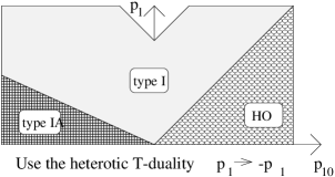
Figure 1: The limits in $d=9$.

For $d=10$ there are only two limits. $p_{0}<0$ gives the heterotic strings and $p_{0}>0$ is the type I theory. However already for $d=9$ we have a more interesting picture analogous to the figure 1 in [1]. Let us make a counterclockwise trip around the figure. We start at a HO point with $p_{1}=0$ which is a weakly coupled heterotic string theory with radii of order $L_{het}$ (therefore it is adjacent to its T-dual region). When we go around the circle, the radius and also the coupling increases and we reach the line $p_{0}\equiv(p_{1}-p_{10})/2=0$ where we must switch to the type I description. Then the radius decreases again so that we must perform a T-duality and switch to the type IA description. This happens for $p_{1}-(p_{0}/2)=(3p_{1}+p_{10})/4=0$; we had to convert $R_{1}$ to the units of $L_{type\,I}=g_{het}^{1/2}L_{het}$. Then we go on and the coupling $g_{IA}$ and/or the size of the line interval increases. The most interesting is the final boundary given by $p_{1}=0$ which guarantees that each of the point of the $p$-space is covered precisely by one limit.

We can show that $p_{1}>0$ is precisely the condition that the dilaton in the type IA theory is not divergent. Roughly speaking, in units of $L_{type\,I}=L_{IA}$ the “gravitational potential” is linear in $x_{1}$ and proportional to $g_{IA}^{2}/g_{IA}$. Here $g_{IA}^{2}$ comes from the gravitational constant and $1/g_{IA}$ comes from the tension of the D8-branes. Therefore we require not only $g_{IA}<1$ but also $g_{IA}<L_{type\,I}/R_{line\,interval}$. Performing the T-duality $L_{type\,I}/R_{line\,interval}=R_{circle}/L_{type\,I}$ and converting to $L_{het}$ the condition becomes precisely $R_{circle}>L_{het}$.

In all the text we adopt (and slightly modify) the standard definition [1] for an asymptotic description to be viable: dimensionless coupling constants should be smaller than one, but in cases without translational invariance, the dilaton should not diverge anywhere, and the sizes of the effective geometry should be greater than the appropriate typical scale (the string length for string theories or the Planck length for M-theory). It is important to realize that in the asymptotic regions we can distinguish between e.g. type I and type IA because their physics is different. We cannot distinguish between them in case the T-dualized circle is of order $L_{type\,I}$ but such vacua are of measure zero in our investigation and form various boundaries in the parameter space. This is the analog of the distinction we made between the IIA and IIB asymptotic toroidal moduli spaces in [1]

2.2 Type IA² and $d=8$

In $d=8$ we will have to use a new desciption to cover the parameter space, namely the double T-dual of type I which we call type IA². Generally, type IA^k contains 16 D-$(9-k)$-branes, their images and $2^{k}$ orientifold $(9-k)$-planes. We find it also useful to perform heterotic T-dualities to make $p_{i}$ positive for $i=1,\dots,10-d$ and sort $p$’s so that our interest is (without a loss of generality) only in configurations with

$$0\leq p_{1}\leq p_{2}\leq\dots\leq p_{10-d}$$ (17)

We need positive $p$’s for the heterotic description to be valid but such a transformation can only improve the situation also for type I and its T-dual descriptions since when we turn $p$’s from negative to positive values, $g_{het}$ increases and therefore $g_{type\,I}$ decreases. For type I we also need large radii. For its T-duals we need a very small string coupling and if we make a T-duality to convert $R>L_{type\,I}$ into $R<L_{type\,I}$, the coupling $g_{IA}$ still decreases; therefore it is good to have as large radii in the type I limit as possible.

In $d=8$ our parameters are $p_{0},p_{1},p_{2}$ or $p_{10},p_{1},p_{2}$ where $p_{10}=-2p_{0}+p_{1}+p_{2}$ and we will assume $0<p_{1}<p_{2}$ as we have explained (sets of measure zero such as the boundaries between regions will be neglected). If $p_{0}<0$, the HO description is good. Otherwise $p_{0}>0$. If furthermore $2p_{1}-p_{0}>0$ (and therefore also $2p_{2}-p_{0}>0$), the radii are large in the type I units and we can use the (weakly coupled) type I description. Otherwise $2p_{1}-p_{0}<0$. If furthermore $2p_{2}-p_{0}>0$, we can use type IA strings. Otherwise $2p_{2}-p_{0}<0$ and the type IA² description is valid. Therefore we cover all the parameter space. Note that the F-theory on K3 did not appear here. In asymptotic moduli space, the F-theory regime generically has no enhanced nonabelian symmetries.

In describing the boundaries of the moduli space, we used the relations $L_{het}=g_{type\,I}^{1/2}L_{type\,I}$, $g_{het}=1/g_{type\,I}$. The condition for the dilaton not to diverge is still $p_{1}>0$ for any type IA^k description. The longest direction of the $T^{k}/{\mathbb{Z}}_{2}$ of this theory is still the most dangerous for the dilaton divergence and is not affected by the T-dualities on the shorter directions of the $T^{k}/{\mathbb{Z}}_{2}$ orientifold. For $d=9$ (and fortunately also for $d=8$) the finiteness of the dilaton field automatically implied that $g_{IA^{k}}<1$. However this is not true for general $d$. After a short chase through a sequence of S and T-dualities we find that the condition $g_{IA^{k}}<1$ can be written as

$$(k-2)p_{0}-2\sum_{i=1}^{k}p_{i}<0.$$ (18)

We used the trivial requirement that the T-dualities must be performed on the shortest radii (if $R_{j}<L_{type\,I}$, also $R_{j-1}<L_{type\,I}$ and therefore it must be also T-dualized). Note that for $k=1$ the relation is $-p_{0}-2p_{1}<0$ which is a trivial consequence of $p_{1}>0$ and $p_{0}>0$. Also for $k=2$ we get a trivial condition $-2(p_{1}+p_{2})<0$. However for $k>2$ this condition starts to be nontrivial. This is neccessary for consistency: otherwise IA^k theories would be sufficient to cover the whole asymptotic moduli space, and because of S-dualities we would cover the space several times. It would be also surprising not to encounter regimes described by large K3 geometries.

2.3 Type IA³, M-theory on K3 and $d=7$

This happens already for $d=7$ where the type IA³ description must be added. The reasoning starts in the same way: for $p_{0}<0$ HO, for $2p_{1}-p_{0}>0$ type I, for $2p_{2}-p_{0}>0$ type IA, for $2p_{3}-p_{0}>0$ type IA².

However, when we have $2p_{3}-p_{0}<0$ we cannot deduce that the conditions for type IA³ are obeyed because also (18) must be imposed:

$$p_{0}-2(p_{1}+p_{2}+p_{3})<0$$ (19)

It is easy to see that this condition is the weakest one i.e. that it is implied by any of the conditions $p_{0}<0$, $2p_{1}-p_{0}>0$, $2p_{2}-p_{0}>0$ or $2p_{3}-p_{0}>0$. Therefore the region that we have not covered yet is given by the opposite equation

$$2p_{0}-4(p_{1}+p_{2}+p_{3})=-p_{10}-3(p_{1}+p_{2}+p_{3})>0$$ (20)

The natural hypothesis is that this part of the asymptotic parameter space is the limit where we can use the description of M-theory on a K3 manifold. However things are not so easy: the condition that $V_{K3}>({L_{planck}^{eleven}})^{4}$ gives just $p_{10}<0$ which is a weaker requirement than (20).

The K3 manifold has a $D_{16}$ singularity but this is not the real source of the troubles. A more serious issue is that the various typical sizes of such a K3 are very different and we should require that each of them is greater than ${L_{planck}^{eleven}}$ (which means that the shortest one is). In an analogous situation with $T^{4}$ instead of K3 the condition $V_{T^{4}}>{L_{planck}^{eleven}}^{4}$ would be also insufficient: all the radii of the four-torus must be greater than ${L_{planck}^{eleven}}$.

Now we would like to argue that the region defined by (20) with our gauge $0<p_{1}<p_{2}<p_{3}$ can indeed be described by the 11D SUGRA on K3, except near the $D_{16}$ singularity. Therefore, all of the asymptotic moduli space is covered by regions which have a reasonable semiclassical description.

While the fourth root of the volume of K3 equals

$$\frac{V_{K3}^{1/4}}{{L_{planck}^{eleven}}}=\frac{g_{het}^{1/3}L_{het}^{1/2}}{V_{3}^{1/6}}=\exp\left(p_{0}/3-(p_{1}+p_{2}+p_{3})/6\right)=\exp(-p_{10}/6),$$ (21)

the minimal typical distance in K3 must be corrected to agree with (20). We must correct it only by a factor depending on the three radii in heterotic units (because only those are the parameters in the moduli space of metric on the K3) so the distance equals (confirming (20))

$$\frac{L_{min.K3}}{{L_{planck}^{eleven}}}=\exp\left(-p_{10}/6-(p_{1}+p_{2}+p_{3})/2\right).$$ (22)

Evidence that (22) is really correct and thus that we understand the limits for $d=7$ is the following. We must first realize that 16 independent two-cycles are shrunk to zero size because of the $D_{16}$ singularity present in the K3 manifold. This singularity implies a lack of understanding of the physics in a vicinity of this point but it does not prevent us from describing the physics in the rest of K3 by 11D SUGRA. So we allow the 16 two-cycles to shrink. The remaining 6 two-cycles generate a space of signature 3+3 in the cohomology lattice: the intersection numbers are identical to the second cohomology of $T^{4}$. We can compute the areas of those 6 two-cycles because the M2-brane wrapped on the 6-cycles are dual to the wrapped heterotic strings and their momentum modes. Now let us imagine that the geometry of the two-cycles of K3 can be replaced by the 6 two-cycles of a $T^{4}$ which have the same intersection number.

It means that the areas can be written as $a_{1}a_{2},a_{1}a_{3},a_{1}a_{4}$, $a_{2}a_{3},a_{2}a_{4},a_{3}a_{4}$ where $a_{1},a_{2},a_{3},a_{4}$ are the radii of the four-torus and correspond to some typical distances of the K3. If we order the $a$’s so that $a_{1}<a_{2}<a_{3}<a_{4}$, we see that the smallest of the six areas is $a_{1}a_{2}$ (the largest two-cycle is the dual $a_{3}a_{4}$) and similarly the second smallest area is $a_{1}a_{3}$ (the second largest two-cycle is the dual $a_{2}a_{4}$). On the heterotic side we have radii $L_{het}<R_{1}<R_{2}<R_{3}$ (thus also $L_{het}^{2}/R_{3}<L_{het}^{2}/R_{2}<L_{het}^{2}/R_{1}<L_{het}$) and therefore the correspondence between the membranes and the wrapping and momentum modes of heterotic strings tells us that

$$\frac{a_{1}a_{2}}{{L_{planck}^{eleven}}^{3}}=\frac{1}{R_{3}},\quad\frac{a_{3}a_{4}}{{L_{planck}^{eleven}}^{3}}=\frac{R_{3}}{L_{het}^{2}},\qquad\frac{a_{1}a_{3}}{{L_{planck}^{eleven}}^{3}}=\frac{1}{R_{2}},\quad\frac{a_{2}a_{4}}{{L_{planck}^{eleven}}^{3}}=\frac{R_{2}}{L_{het}^{2}}.$$ (23)

As a check, note that $V_{K3}=a_{1}a_{2}a_{3}a_{4}$ gives us ${L_{planck}^{eleven}}^{6}/L_{het}^{2}$ as expected (since heterotic strings are M5-branes wrapped on $K3$). We will also assume that

$$\frac{a_{1}a_{4}}{{L_{planck}^{eleven}}^{3}}=\frac{1}{R_{1}},\quad\frac{a_{2}a_{3}}{{L_{planck}^{eleven}}^{3}}=\frac{R_{1}}{L_{het}^{2}}.$$ (24)

Now we can calculate the smallest typical distance on the K3.

$$a_{1}=\sqrt{\frac{a_{1}a_{2}\cdot a_{1}a_{3}}{a_{2}a_{3}}}=\frac{{L_{planck}^{eleven}}^{3/2}L_{het}}{\sqrt{R_{1}R_{2}R_{3}}}$$ (25)

which can be seen to coincide with (22). There is a subtlety that we should mention. It is not completely clear whether $a_{1}a_{4}<a_{2}a_{3}$ as we assumed in (24). The opposite possibility is obtained by exchanging $a_{1}a_{4}$ and $a_{2}a_{3}$ in (24) and leads to $a_{1}$ greater than (25) which would imply an overlap with the other regions. Therefore we believe that the calculation in (24) and (25) is the correct way to find the condition for the K3 manifold to be large enough for the 11-dimensional supergravity (as a limit of M-theory) to be a good description.

2.4 Type IA^4,5, type IIA/B on K3 and $d=6,5$

Before we will study new phenomena in lower dimensions, it is useful to note that in any dimension we add new descriptions of the physics. The last added limit always corresponds to the “true” S-dual of the original heterotic string theory – defined by keeping the radii fixed in the heterotic string units (i.e. also keeping the shape of the K3 geometry) and sending the coupling to infinity – because this last limit always contains the direction with $p_{0}$ large and positive (or $p_{10}$ large and negative) and other $p_{i}$’s much smaller.

• In 10 dimensions, the true S-dual of heterotic strings is the type I theory.

• In 9 dimensions it is type IA.

• In 8 dimensions type IA².

• In 7 dimensions we get M-theory on K3.

• In 6 dimensions type IIA strings on K3.

• In 5 dimensions type IIB strings on K3$\times S^{1}$ where the circle decompactifies as the coupling goes to infinity. The limit is therefore a six-dimensional theory.

• In 4 dimensions we observe a mirror copy of the region $p_{10}<0$ to arise for $p_{10}>0$. The strong coupling limit is the heterotic string itself.

• In 3 dimensions the dilaton-axion is already unified with the other moduli so it becomes clear that we studied an overly specialized direction in the examples above. Nevertheless the same claim as in $d=4$ can be made.

• In 2 dimensions only positive values of $p_{10}$ are possible therefore the strong coupling limit does not exist in the safe domain of moduli space.

• In 1 dimension the Lorentzian structure of the parameter space emerges. Only the future light cone corresponds to semiclassical physics which is reasonably well understood. The strong coupling limit defined above would lie inside the unphysical past light cone.

Now let us return to the discussion of how to separate the parameter space into regions where different semiclassical descriptions are valid. We may repeat the same inequalities as in $d=7$ to define the limits HO, I, IA, IA², IA³. But for M-theory on K3 we must add one more condition to the constraint (20): a new circle has been added and its size should be also greater than ${L_{planck}^{eleven}}$. For the new limit of the type IIA strings on K3 we encounter similar problems as in the case of the M-theory on K3. Furthermore if we use the definition (22) and postulate this shortest distance to be greater than the type IIA string length, we do not seem to get a consistent picture covering the whole moduli space. Similarly for $d=5$, there appear two new asymptotic descriptions, namely type IA⁵ theory and type IIB strings on $K3\times S^{1}$. It is clear that the condition $g_{IA^{5}}<1$ means part of the parameter space is not understood and another description, most probably type IIB strings on $K3\times S^{1}$, must be used. Unfortunately at this moment we are not able to show that the condition for the IIB theory on K3 to be valid is complementary to the condition $g_{IA^{5}}<1$. A straightforward application of (25) already for the type IIA theory on a K3 gives us a different inequality. Our lack of understanding of the limits for $d<7$ might be solved by employing a correct T-duality of the type IIA on K3 but we do not have a complete and consistent picture at this time.

2.5 Type IA⁶ and S-duality in $d=4$

Let us turn to the questions that we understand better. As we have already said, in $d=4$ we see the ${\mathbb{Z}}_{2}$ subgroup of the $SL(2,{\mathbb{Z}})$ S-duality which acts as $p_{10}\to-p_{10}$ and $p_{1},\dots,p_{6}$ fixed in our formalism. This reflection divides the $p$-space to subregions $p_{10}>0$ and $p_{10}<0$ which will be exchanged by the S-duality. This implies that a new description should require $p_{10}>0$. Fortunately this is precisely what happens: in $d=4$ we have one new limit, namely the type IA⁶ strings and the condition (18) for $g_{IA^{6}}<1$ gives

$$4p_{0}-2\sum_{i=1}^{6}p_{i}=-2p_{10}<0$$ (26)

or $p_{10}>0$.

In the case of $d=3$ we find also a fundamental domain that is copied several times by S-dualities. This fundamental region is again bounded by the condition $g_{gauge}^{eff.4-dim}<1$ which is the same like $g_{IA^{6}}<1$ and the internal structure has been partly described: the fundamental region is divided into several subregions HO, type I, type IA^k, M/K3, IIA/K3, IIB/K3. As we have said, we do not understand the limits with a K3 geometry well enough to separate the fundamental region into the subregions enumerated above. We are not even sure whether those limits are sufficient to cover the whole parameter space. In the case of $E_{8}\times E_{8}$ theory, we are pretty sure that there are some limits that we do not understand already for $d=9$ and similar claim can be true in the case of the $SO(32)$ vacua for $d<7$. We understand much better how the entire parameter space can be divided into the copies of the fundamental region and we want to concentrate on this question.

The inequality $g_{gauge}^{eff.4-dim}<1$ should hold independently of which of the six radii are chosen to be the radii of the six-torus. In other words, it must hold for the smallest radii and the condition is again (26) which can be for $d=3$ reexpressed as $p_{7}<p_{10}$.

So the “last” limit at the boundary of the fundamental region is again type IA⁶ and not type IA⁷, for instance. It is easy to show that the condition $g_{IA^{6}}<1$ is implied by any of the conditions for the other limits so this condition is the weakest of all: all the regions are inside $g_{IA^{6}}<1$.

This should not be surprising, since $g_{gauge}^{eff.4-dim}=(g_{IA^{6}})^{1/2}=g_{IA^{6}}^{open}$; the heterotic S-duality in this type IA⁶ limit can be identified with the S-duality of the effective low-energy description of the D3-branes of the type IA⁶ theory. As we have already said, this inequality reads for $d=3$

$$2p_{0}-\sum_{i=1}^{6}p_{i}=-p_{10}+p_{7}<0$$ (27)

or $p_{10}>p_{7}$. We know that precisely in $d=3$ the S-duality (more precisely the $ST^{6}$ transformation) acts as the permutation of $p_{7}$ and $p_{10}$. Therefore it is not hard to see what to do if we want to reach the fundamental domain: we change all signs to pluses by T-dualities and sort all eight numbers $p_{1},\dots p_{7};p_{10}$ in the ascending order. The inequality (27) will be then satisfied. The condition $g_{gauge}^{eff.4-dim}<1$ or (26) will define the fundamental region also for the case of one or two dimensions.

2.6 The infinite groups in $d\leq 2$

In the dimensions $d>2$ the bilinear form is positive definite and the group of dualities conserves the lattice ${\mathbb{Z}}^{11-d}$ in the $p$-space. Therefore the groups are finite. However for $d=2$ (and a fortiori for $d=1$ because the $d=2$ group is isomorphic to a subgroup of the $d=1$ group) the group becomes infinite. In this dimension $p_{10}$ is unchanged by T-dualities and S-dualities. The regions with $p_{10}\leq 0$ again correspond to mysterious regions where the holographic principle appears to be violated, as in [1]. Thus we may assume that $p_{10}=1$; the overall normalization does not matter.

Start for instance with $p_{10}=1$ and

$$(p_{1},p_{2},\dots p_{8})=(0,0,0,0,0,0,0,0)$$ (28)

and perform the S-duality ($ST^{6}$ from the formula (15)) with $p_{7}$ and $p_{8}$ understood as the large dimensions (and $p_{1}\dots p_{6}$ as the 6-torus). This transformation maps $p_{7}\mapsto p_{10}-p_{8}$ and $p_{8}\mapsto p_{10}-p_{7}$. So if we repeat $ST^{6}$ on $p_{7},p_{8}$, T-duality of $p_{7},p_{8}$, $ST^{6}$, $T^{2}$ and so on, $p_{1}\dots p_{6}$ will be still zero and the values of $p_{7},p_{8}$ are

$$(p_{7},p_{8})=(1,1)\to(-1,-1)\to(2,2)\to(-2,-2)\to(3,3)\to\dots$$ (29)

and thus grow linearly to infinity, proving the infinite order of the group. The equation for $g_{IA^{6}}<1$ now gives

$$2p_{0}-\sum_{i=1}^{6}p_{i}=-p_{10}+p_{7}+p_{8}<0$$ (30)

or $p_{10}>p_{7}+p_{8}$. Now it is clear how to get to such a fundamental region with (30) and $0<p_{1}<\dots p_{8}$. We repeat the $ST^{6}$ transformation with the two largest radii ($p_{7},p_{8}$) as the large coordinates. After each step we turn the signs to $+$ by T-dualities and order $p_{1}<\dots<p_{8}$ by permutations of radii. A bilinear quantity decreases assuming $p_{10}>0$ and $p_{10}<p_{7}+p_{8}$ much like in [1], the case $k=9$ ($d=2$):

$$C_{d=2}=\sum_{i=1}^{8}(p_{i})^{2}\to\sum_{i=1}^{8}(p_{i})^{2}+2p_{10}(p_{10}-(p_{7}+p_{8}))$$ (31)

In the same way as in [1], starting with a rational approximation of a vector $\vec{p}$, the quantity $C_{d=2}$ cannot decrease indefinitely and therefore finally we must get to a point with $p_{10}>p_{7}+p_{8}$.

In the case $d=1$ the bilinear form has a Minkowski signature. The fundamental region is now limited by

$$2p_{0}-\sum_{i=1}^{6}p_{i}=-p_{10}+p_{7}+p_{8}+p_{9}<0$$ (32)

and it is easy to see that under the $ST^{6}$ transformation on radii $p_{1}\dots p_{6}$, $p_{10}$ transforms as

$$p_{10}\to 2p_{10}-(p_{7}+p_{8}+p_{9}).$$ (33)

Since the $ST^{6}$ transformation is a reflection of a spatial coordinate in all cases, it keeps us inside the future light cone if we start there. Furthermore, after each step we make such T-dualities and permutations to ensure $0<p_{1}<\dots p_{9}$.

If the initial $p_{10}$ is greater than $[(p_{1})^{2}+\dots+(p_{9})^{2}]^{1/2}$ (and therefore positive), it remains positive and assuming $p_{10}<p_{7}+p_{8}+p_{9}$, it decreases according to (33). But it cannot decrease indefinitely (if we approximate $p$’s by rational numbers or integers after a scale transformation). So at some point the assumption $p_{10}<p_{7}+p_{8}+p_{9}$ must break down and we reach the conclusion that fundamental domain is characterized by $p_{10}>p_{7}+p_{8}+p_{9}$.

2.7 The lattices

In the maximally supersymmetric case [1], we encountered exceptional algebras and their corresponding lattices. We were able to see some properties of the Weyl group of the exceptional algebra $E_{10}$ and define its fundamental domain in the Cartan subalgebra. In the present case with 16 supersymmetries, the structure of lattices for $d>2$ is not as rich. The dualities always map integer vectors $p_{i}$ onto integer vectors.

For $d>4$, there are no S-dualities and our T-dualities know about the group $O(26-d,10-d,{\mathbb{Z}})$. For $d=4$ our group contains an extra ${\mathbb{Z}}_{2}$ factor from the single S-duality. For $d=3$ they unify to a larger group $O(8,24,{\mathbb{Z}})$. We have seen the semidirect product of $({\mathbb{Z}}_{2})^{8}$ and $S_{8}$ related to its Weyl group in our formalism. For $d=2$ the equations of motion exhibit a larger affine $\hat{o}(8,24)$ algebra whose discrete duality group has been studied in [3].

In $d=1$ our bilinear form has Minkowski signature. The S-duality can be interpreted as a reflection with respect to the vector

$$(p_{1},p_{2},\dots,p_{9},p_{10})=(0,0,0,0,0,0,-1,-1,-1,+1).$$ (34)

This is a spatial vector with length-squared equal to minus two (the form (3) has a time-like signature). As we have seen, such reflections generate together with T-dualities an infinite group which is an evidence for an underlying hyperbolic algebra analogous to $E_{10}$. Indeed, Ganor [5] has argued that the $DE_{18}$ “hyperbolic” algebra underlies the nonperturbative duality group of maximally compactified heterotic string theory. The Cartan algebra of this Dynkin diagram unifies the asymptotic directions which we have studied with compact internal symmetry directions. Its Cartan metric has one negative signature direction.

3 Conclusions

The parallel structure of the moduli spaces with 32 and 16 SUSYs gives us reassurance that the features uncovered in [1] are general properties of M-theory. It would be interesting to extend these arguments to moduli spaces with less SUSY. Unfortunately, we know of no algebraic characterization of the moduli space of M-theory on a Calabi Yau threefold. Furthermore, this moduli space is no longer an orbifold. It is stratified, with moduli spaces of different dimensions connecting to each other via extremal transitions. Furthermore, in general the metric on moduli space is no longer protected by nonrenormalization theorems, and we are far from a characterization of all the extreme regions. For the case of four SUSYs the situation is even worse, for most of what we usually think of as the moduli space actually has a superpotential on it, which generically is of order the fundamental scale of the theory.

There are thus many hurdles to be jumped before we can claim that the concepts discussed here and in [1] have a practical application to realistic cosmologies.

- [1] T. Banks, W. Fischler, L. Motl, Dualities versus singularities, J. High Energy Phys. 01 (1999) 019 [hep-th/9811194].
- [2] A. Sen, Strong-weak coupling duality in three-dimensional string theory, Nucl. Phys. B 434 (1995) 179-209 [hep-th/9408083].
- [3] A. Sen, Duality symmetry group of two-dimensional heterotic string theory, Nucl. Phys. B 447 (1995) 62-84 [hep-th/9503057].
- [4] J.H. Schwarz, Classical duality symmetries in two dimensions, hep-th/9505170.
- [5] O. Ganor, Two conjectures on gauge theories, gravity, and infinite dimensional Kac-Moody groups, hep-th/9903110.
- [6] T. Banks, M. Dine, Quantum moduli spaces of string theories, Phys. Rev. D 53 (5790) 1996 [hep-th/9508071].