KCL-MTH-99-10

DTP–99/23

hep-th/9904002

Particle Reflection Amplitudes
in $a_{n}^{(1)}$ Toda Field Theories
G. W. Delius and G. M. Gandenberger
^aDepartment of Mathematics
King’s College London
Strand, London WC2R 2LS, U.K.
^bDepartment of Mathematical Sciences
Durham University
Durham DH1 3LE, U.K.
ABSTRACT

We determine the exact quantum particle reflection amplitudes for all known vacua of $a_{n}^{(1)}$ affine Toda theories on the half-line with integrable boundary conditions. (Real non-singular vacuum solutions are known for about half of all the classically integrable boundary conditions.) To be able to do this we use the fact that the particles can be identified with the analytically continued breather solutions, and that the real vacuum solutions are obtained by analytically continuing stationary soliton solutions. We thus obtain the particle reflection amplitudes from the corresponding breather reflection amplitudes. These in turn we calculate by bootstrapping from soliton reflection matrices which we obtained as solutions of the boundary Yang-Baxter equation (reflection equation).

We study the pole structure of the particle reflection amplitudes and uncover an unexpectedly rich spectrum of excited boundary states, created by particles binding to the boundary. For $a_{2}^{(1)}$ and $a_{4}^{(1)}$ Toda theories we calculate the reflection amplitudes for particle reflection off all these excited boundary states. We are able to explain all physical strip poles in these reflection factors either in terms of boundary bound states or a generalisation of the Coleman-Thun mechanism.

1 Introduction and Overview

The study of two-dimensional integrable quantum field theories is interesting because it allows one to calculate exactly things like the quantum behaviour of solitons, the weak–strong coupling duality, the effects of space-time boundaries, etc. Exact studies in two dimensions allow one to speculate more confidently about these phenomena also in higher dimensions. A particularly rewarding class of integrable quantum field theories to study are the affine Toda field theories (ATFTs). Some of their nice features include: they exhibit weak–strong coupling duality, they have quantum group symmetries [2], they have solitons and breathers [30, 33], and, most importantly for this paper, they have a rich set of integrable boundary conditions [11, 3].

For the particles of real coupling affine Toda theories without boundaries it has been possible to find the exact S-matrices, describing the evolution of arbitrary asymptotic incoming particle states into asymptotic outgoing particle states [1, 5, 8, 15]. It has been a longstanding challenge to extend these results to the half-line with integrable boundary conditions.

We will only deal with $a_{n}^{(1)}$ Toda theory in this paper. The classical equation of motion for the $n$-component bosonic field of $a_{n}^{(1)}$ Toda theory is

$$\partial_{t}^{2}{{\boldsymbol{\phi}}}-\partial_{x}^{2}{{\boldsymbol{\phi}}}+\frac{m^{2}}{\beta}\sum_{i=0}^{n}{\boldsymbol{\alpha}}_{i}e^{\beta{\boldsymbol{\alpha}}_{i}\cdot{\boldsymbol{\phi}}}=0.$$ (1.1)

The $\alpha_{i}$, $i=1,\cdots,n$ are the simple roots of the Lie algebra $a_{n}=\text{sl}_{n+1}$ and $\alpha_{0}$ is minus the highest root. We will use units so that the mass scale $m=1$. Note that the coupling constant $\beta$ could be removed from the equations of motion by rescaling the field and therefore the coupling constant plays a role only in the quantum theory.

It has been discovered in [11, 3] that this equation of motion can be restricted to the left half-line $x<0$ without losing integrability if one imposes a boundary condition at $x=0$ of the form

$$\left.\beta\,\partial_{x}{\boldsymbol{\phi}}+\sum_{i=0}^{n}C_{i}\,{\boldsymbol{\alpha}}_{i}e^{\beta{\boldsymbol{\alpha}}_{i}\cdot{\boldsymbol{\phi}}/2}\right|_{x=0}=0,$$ (1.2)

where the boundary parameters $C_{i}$ satisfy either

$$C_{i}=0\;,\hskip 28.45274pt(i=0,1,\dots,n)\;,$$ (1.3)

which gives the Neumann boundary condition, or

$$C_{i}=\pm 1\;,\hskip 28.45274pt(i=0,1,\dots,n)\;,$$ (1.4)

which will be denoted as the (++…– –…) boundary conditions.

The original ideas needed to determine the full S-matrix in the presence of integrable boundary conditions are due to Cherednik [7], Ghoshal and Zamolodchikov[28] and Fring and Köberle[21]. As a consequence of the higher-spin symmetries of affine Toda theory all amplitudes factorise into products of the two-particle scattering amplitudes and the single-particle reflection amplitudes. These amplitudes in turn are strongly restricted by the requirements of real analyticity, unitarity, crossing symmetry and the bootstrap equations. We recall some details regarding this in section 2.

If one knows the spectrum of the integrable theory under investigation, these constraints are usually strong enough to determine the amplitudes uniquely. This explains the success in finding the S-matrices for affine Toda theories on the whole line, because one can read off the particle spectrum directly from the Lagrangian. In a theory on the half-line however a large number of boundary bound states can exist in addition to the particle states. Unfortunately there is no obvious way how to read off the spectrum of boundary states directly from the Lagrangian. This is the reason why many previous attempts to determine the reflection amplitudes relying only on the above mentioned constraints have failed. We will see below that the correct reflection factors have a rather intricate boundary state spectrum.

The new approach to finding the particle reflection amplitudes which we will use in this paper has been proposed in [26]. It is based on an earlier discovery that the lowest breather states in imaginary coupling Toda theory can be identified with the fundamental particles in the real coupling theory in the sense that the particle S-matrices are obtained from the breather S-matrices by analytic continuation in the coupling constant [23, 24]. Previously this phenomenon was only known to be exhibited by the sine-Gordon model. In [26] it was proposed that the same should also hold for the reflection amplitudes. Analytic continuation of the breather reflection amplitudes should give the particle reflection amplitudes.

The breather reflection amplitudes are determined by bootstrap from the reflection amplitudes of the constituent solitons. The soliton reflection amplitudes in turn can be obtained by solving the reflection equation which is the analogue of the Yang-Baxter equation for reflection amplitudes. In [26] the reflection equation for $a_{2}^{(1)}$ Toda theory was solved and the particle reflection amplitudes for $a_{2}^{(1)}$ Toda theory with Neumann or $(+++)$ boundary condition were calculated. The results are briefly recalled and then generalised to $a_{n}^{(1)}$ Toda theory with arbitrary $n$ in section 3. We obtain the reflection amplitudes for the uniform $(++\cdots++)$ boundary condition in eq.(3.16) and find that they confirm an early conjecture made in [11]. The reflection amplitudes for the Neumann boundary condition, which we conjecture to be obtained by duality, are given in eq.(3.20).

A prerequisite for progress towards deriving the reflection amplitudes for the other integrable boundary conditions was an understanding of their classical vacuum solutions. Bowcock [4] determined these vacuum solutions for $a_{n}^{(1)}$ Toda theories. This study of classical solutions was simplified and generalised in [16]. It was found that for about half of all integrable boundary conditions in $a_{n}^{(1)}$ Toda theory real-valued vacuum solutions can be obtained by analytically continuing a solution describing a stationary soliton in front of the boundary. We therefore call these boundary conditions ‘solitonic’. Some details of this are given in section 4. With this knowledge it is then easy to obtain the particle reflection amplitudes for the vacuum states for these boundary conditions. This is done in section 5. We find that the boundary conditions fall into $\lfloor(n+1)/2\rfloor$ equivalence classes (where $\lfloor k\rfloor$ is the integer part of $k$). Namely all boundary conditions whose vacuum solutions are obtained from solitons in the same multiplet or from solitons in the conjugate multiplet give rise to the same reflection amplitudes. The result for the reflection amplitudes can be found in eqs. (5.5), (5.4).

In section 6 we study the pole structure of these reflection amplitudes. This constitutes most of the work in this paper. We discover that the vacuum reflection factors have simple poles which imply the existence of excited boundary states. We can obtain the amplitudes for reflection off these excited boundaries by using the boundary bootstrap equations. These in turn have new poles implying the existence of yet more excited boundary states.

We have performed this analysis in detail for the cases of the $a_{2}^{(1)}$ and $a_{4}^{(1)}$ Toda theories. In each of these cases we end up with an array of boundary states. The number of excited boundary states grows as the coupling constant becomes smaller. As an example we have plotted in figures 1 and 2 the spectrum of boundary states for the solitonic boundary conditions of $a_{2}^{(1)}$ affine Toda theory at two different values of the coupling constant $B=\frac{\beta^{2}}{2\pi}/(1+\frac{\beta^{2}}{4\pi})$. In figure 1 we have also indicated which particle has to bind to the boundary to go from one state to the other by labels on the lines connecting the states. A more illuminating animated plot of the spectrum can be found on this paper’s web site at http//www.mth.kcl.ac.uk/~delius/pub/reflection.html.

Figure 1: The spectrum of boundary states for $a_{2}^{(1)}$ Toda theory with a solitonic boundary condition at coupling constant $B\approx\frac{1}{2}$. The vertical axis is the boundary state energy.

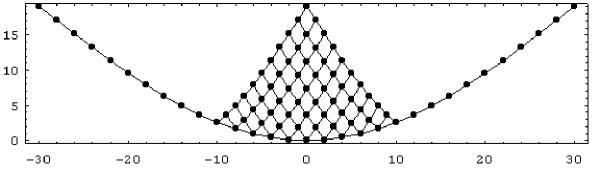
Figure 2: As the coupling constant becomes smaller, the number of boundary states grows. This plot shows the spectrum as in figure 1 but at coupling constant $B\approx\frac{1}{10}$.

The amplitudes for the reflection of the particles off these boundary states are given explicitly in eq.(6.7) for $a_{2}^{(1)}$, in eqs. (6.4.1) and (6.4.1) for the first class of boundary conditions in $a_{4}^{(1)}$ and eqs. (6.4.2) and (6.4.2) for the second class. We have also begun the analysis for $a_{3}^{(1)}$ in section 6.3.

In these reflection amplitudes there are also a large number of physical strip poles which do not correspond to new bound states but have an explanation in terms of a boundary generalisation [20] of the Coleman-Thun mechanism [9]. The way in which this works conveys the strong impression that there is some magic at work which awaits a deeper explanation.

2 Exact S-matrices and reflection amplitudes

This section gives a brief review of the properties of particle S-matrices and reflection amplitudes and the consistency equations which they are subject to. For an excellent presentation of this material see [13].

The reason why the full S-matrices of affine Toda theories can be determined exactly is that these theories possess higher-spin symmetries. A higher-spin symmetry implies that the sum of some power of the momenta of the particles is conserved during scattering. This allows only processes in which the incoming particles have the same momenta as the outgoing ones. Furthermore a higher-spin symmetry acts on the particles by shifting them by amounts proportional to powers of their momenta. This allows one to separate the interaction regions as illustrated in figure 3. This implies that any S-matrix factorizes into a product of 2-particle S-matrices.

Figure 3: Higher-spin symmetries allow one to shift the different particle trajectories independently, thereby separating multi-particle scattering processes into products of two-particle scatterings.

If the particles live on a half-line, then in addition to scattering with each other they are also going to reflect off the boundary. Ideally one would hope that a multi-particle process will now factorise into a succession of two-particle scatterings and single-particle reflections off the boundary, as depicted in figure 4.

Figure 4: In the presence of an integrable boundary any multi-particle process factorises into a product of two-particle scatterings and single-particle reflections.

Of course all momentum-dependent translation symmetries in the space direction will be broken by the boundary. However one can choose the boundary condition in such a way that it preserves those parts of the higher-spin-symmetries which effect momentum-dependent translations in the time direction and these suffice to separate the interaction regions. Thus in order to determine the full S-matrix on the half-line we only need the single-particle reflection matrices and the two-particle S-matrices. The later will not be changed by the presence of the boundary because the particle scatterings could be shifted arbitrarily far away from the boundary.

In affine Toda theory all particles are distinguished by their masses and higher-spin charges and therefore the S-matrix has to be diagonal.

(2.1)

We have introduced the rapidity variable $\theta$ which is related to the momentum components by

$$E=m\cosh\theta,~{}~{}~{}~{}p=m\sinh\theta,$$ (2.2)

where $m$ is the mass of the particle. We draw the worldline of a particle with rapidity $\theta$ at an angle of $u=-i\theta$ to the vertical.

Depending on which of the higher-spin symmetries remain unbroken by the boundary condition a particle has to be reflected either into itself or into its antiparticle. We will find that for the boundary conditions which we study the former is the case and so the reflection matrices are diagonal

(2.3)

The scattering and the reflection amplitudes have to be unitary, real analytic and $2\pi i$-periodic. This implies that they can be written as a product of fundamental building blocks (we use the notation of [5] in which $h=n+1$ is the Coxeter number of $a_{n}^{(1)}$)

$$\biggl{(}x\biggr{)}\equiv\frac{\sin\left(\frac{\theta}{2i}+\frac{\pi}{2h}x\right)}{\sin\left(\frac{\theta}{2i}-\frac{\pi}{2h}a\right)},$$ (2.4)

$$S_{ab}(\theta)=\prod_{x\in A_{ab}}\biggl{(}x\biggr{)}\,,~{}~{}~{}~{}~{}~{}K_{a}(\theta)=\prod_{x\in B_{a}}\biggl{(}x\biggr{)}\;.$$ (2.5)

Each block $(x)$ has a pole at $\theta=x\,i\pi/h$ and a zero at $\theta=-x\,i\pi/h$. Thus the problem of calculating the full exact S-matrix has been reduced to the task of finding the sets $A_{ab}$ and $B_{a}$ of numbers specifying the locations of the poles and zeros in the two-particle scattering amplitudes $S_{ab}$ and the reflection amplitudes $K_{a}$ respectively.

As an illustration we give the scattering amplitudes for $a_{2}^{(1)}$ affine Toda theory which we will meet again in section 6.2. This theory has two conjugate particles of equal mass with scattering amplitudes

$$S_{11}=S_{22}=\biggl{(}-2+B\biggr{)}\,\biggl{(}-B\biggr{)}\,\biggl{(}2\biggr{)}\,,$$ (2.6)

$$S_{12}=S_{21}=-\,\biggl{(}-3+B\biggr{)}\,\biggl{(}-1-B\biggr{)}\,\biggl{(}1\biggr{)}\,.$$ (2.7)

Here $B$ is the usual coupling constant dependent function

$$B(\beta)=\frac{1}{2\pi}\frac{\beta^{2}}{1+\frac{\beta^{2}}{4\pi}}\;,$$ (2.8)

The reflection amplitudes depend on which integrable boundary condition we choose. For example for the solitonic boundary condition dealt with in section 6.2 we have

$$K_{1}=K_{2}=\biggl{(}-2\biggr{)}\,\biggl{(}-\frac{B}{2}\biggr{)}\,\biggl{(}2+\frac{B}{2}\biggr{)}\,\biggl{(}\frac{1}{2}-\frac{B}{2}\biggr{)}\,\biggl{(}\frac{3}{2}-\frac{B}{2}\biggr{)}\,\biggl{(}\frac{3}{2}+\frac{B}{2}\biggr{)}\,\biggl{(}\frac{5}{2}+\frac{B}{2}\biggr{)}\;.$$ (2.9)

Crossing symmetry relates different amplitudes to each other,

$$S_{ab}(\theta)=S_{b\bar{a}}(i\pi-\theta),~{}~{}~{}~{}~{}K_{a}(\theta)K_{\bar{a}}(\theta+i\pi)=S_{aa}(2\theta),$$ (2.10)

where $\bar{a}$ denotes the antiparticle to $a$ and is given for $a_{n}^{(1)}$ Toda theory by $\bar{a}=h-a$. The second of these relations was first derived by Ghoshal and Zamolodchikov [28]. It can be checked that the example given above satisfies these crossing relations by using the following properties of the blocks:

$$\biggl{(}a\biggr{)}_{\theta+i\pi}=-\biggl{(}a+h\biggr{)},~{}~{}~{}~{}\biggl{(}a\biggr{)}_{2\theta}=-\biggl{(}\frac{a}{2}\biggr{)}\,\biggl{(}\frac{a}{2}+h\biggr{)},~{}~{}~{}~{}\biggl{(}a\biggr{)}_{-\theta}=-\biggl{(}a\biggr{)}^{-1}.$$ (2.11)

By going from the Mandelstamm variable $s$ to the relative rapidity variable $\theta$ the physical sheet has been mapped to the physical strip $0<Im(\theta)<\pi$ (see for example [37] for details). Every pole on the physical strip has to have a physical explanation. In the example above the amplitude $S_{11}$ has a pole from the block $(2)$ at $\theta=2i\pi/3$ which corresponds to the propagation of a particle of type $2$ in the forward channel, as depicted in figure 5 a).

Figure 5: a) Simple poles in a scattering amplitude may be due to the propagation of a bound state. b) Simple poles in a reflection amplitude may be due to the formation of an excited boundary state.

A further consequence of the higher-spin symmetries and the corresponding momentum-dependent translation of particle lines is the bootstrap principle. It expresses the scattering amplitudes for bound states in terms of those of the constituent particles. For example the bound state pole discussed above leads to the following bootstrap equation which gives $S_{12}$ in terms of $S_{11}$,

(2.12)

This provides an independent consistency check on the amplitude $S_{12}$ given in (2.7) which was already determined by crossing symmetry. In practice there is a large number of such bootstrap consistency equations and these, together with the requirement that any pole on the physical strip needs to have a physical explanation, are strong enough to determine the S-matrices of all affine Toda theories uniquely.

Similar relations exist for the reflection amplitudes. Firstly there is a bootstrap equation relating the reflection amplitudes of the different particles to each other, depicted in figure 7. Secondly every pole on the physical strip requires a physical explanation. For reflection amplitudes the physical strip in the rapidity plane is bounded by $Im(\theta)\leq\pi/2$. Our example in (2.9) has two simple poles on the physical strip, namely at $\theta=i\frac{\pi}{3}\left(\frac{1}{2}-\frac{B}{2}\right)$ and at $\theta=i\frac{\pi}{3}\left(\frac{3}{2}-\frac{B}{2}\right)$. These correspond to the propagation of excited boundary states as illustrated in figure 5 b). The reflection amplitudes for reflection of these excited boundaries is determined by the following bootstrap equation,

(2.13)

The bootstrap equations would probably again be strong enough to determine the reflection amplitudes uniquely if one knew the spectrum of excited boundary states a priori. However this is not easy to derive directly and therefore we took a different route, to be described below.

Not only tree diagrams as those in figure 5 give rise to poles on the physical strip. Rather any Feynman diagram in which some internal lines are on-shell can produce poles. For example the box diagram in figure 6a) will lead to a second order pole if all the internal lines can be simultaneously on shell (which does not happen in $a_{2}^{(1)}$ but in higher Toda theories). The order of the pole is determined by the number of lines on shell minus twice the number of loop integrations. The boundary diagram in figure 6(b) has six internal lines and two loop momenta and will thus generically lead to a second order pole unless the reflection amplitude in the middle of the diagram does itself have poles or zeros at this point. This boundary generalisation of the Coleman-Thun mechanism [9] was discovered by Dorey et.al. in [20].

Figure 6: Diagrams with internal lines on shell lead to additional poles on the physical strip.

Thus to check a conjectured amplitude one should draw all possible diagrams which can have internal lines on shell, determine what kind of poles they lead to, and then compare with the pole structure of the conjectured amplitude. These checks have been carefully performed for the scattering amplitudes of affine Toda theory on the whole line. We will do the same for our reflection amplitudes for $a_{2}^{(1)}$ and $a_{4}^{(1)}$ Toda theory in section 6 and will find that it works quite miraculously. A similar analysis has been performed for the reflection amplitudes in the boundary scaling Lee-Yang model [20].

3 Reflection amplitudes for Neumann and $(++\cdots++)$ boundary conditions

3.1 Reflection in $a_{2}^{(1)}$ ATFT revisited

In a recent paper [26] one of us constructed reflection amplitudes for $a_{2}^{(1)}$ ATFT. We briefly recall the main results of this work here.

The construction was based on new solutions to the $a_{2}^{(1)}$ boundary Yang-Baxter equation (BYBE). Some of these new solutions, the so-called $K$-matrices, were conjectured to describe the reflection of the fundamental solitons in imaginary coupling $a_{2}^{(1)}$ ATFT. By comparison with semi-classical calculations [16] it was possible to identify the two reflection matrices which correspond to the Neumann and the uniform (+++) boundary conditions. Using the boundary bootstrap equations, the reflection amplitudes for the breathers in the theory were constructed. Due to the identification of the lowest breathers in the imaginary coupling theory with the fundamental particles in the real coupling theory, it was then possible to find the reflection amplitudes for the particles in the real coupling $a_{2}^{(1)}$ ATFT via a simple analytic continuation.

This led to the following particle reflection amplitudes, corresponding to the Neumann and the uniform (+++) boundary conditions respectively,

$$K^{N}_{1}(\theta)=K^{N}_{2}(\theta) = \biggl{(}-2\biggr{)}\,\biggl{(}-\frac{B}{2}\biggr{)}\,\biggl{(}2+\frac{B}{2}\biggr{)}\;,$$ (3.1)

$$K_{1}(\theta)=K_{2}(\theta) = \biggl{(}-2\biggr{)}\,\biggl{(}\frac{B}{2}-1\biggr{)}\,\biggl{(}3-\frac{B}{2}\biggr{)}\;,$$ (3.2)

in which the brackets are defined as in (2.4) with $h=3$. These amplitudes are in agreement with classical and semi-classical calculations [12, 31, 34].

Given that the $S$-matrices in the bulk theory have long been known to be self-dual under a weak–strong coupling duality, it was widely expected that a duality like that can also be found in ATFT on a half-line. However, the above reflection amplitudes are not self-dual, but instead are dual to each other, i.e.

$$K^{N}_{1}(\theta)\longleftrightarrow K_{1}(\theta)\;,\hskip 56.9055pt(\mbox{as}\;\;\;\beta\longleftrightarrow\frac{4\pi}{\beta})\;.$$ (3.3)

This generalises the analogous result in the sinh-Gordon theory in [14].

In the following we demonstrate how these results can be generalised to the case of $a_{n}^{(1)}$ ATFTs. Just as in the $a_{2}^{(1)}$ case, our construction of particle reflection amplitudes begins with proposing a reflection matrix for the fundamental solitons in imaginary coupling ATFT with uniform $(++\cdots++)$ boundary condition.

3.2 Notation

We use the notation of [24]. Whenever we deal with solitons or breathers, we use the following parametrisation of the rapidity:

$$\mu=-i\frac{h\lambda}{2\pi}\theta\;,$$

and the bracket notation

$$\biggl{(}a\biggr{)}_{I}\equiv\frac{\left[a\right]}{\left[-a\right]}\;,\;\;\;\;\;\;\;\;\;\;\left[a\right]\equiv\sin\left(\frac{\pi}{h\lambda}(\mu+a)\right)\;,$$ (3.4)

in which $h=n+1$ is the Coxeter number of the affine Lie algebra $a_{n}^{(1)}$, and $\lambda$ is related to the imaginary Toda coupling constant $\beta$ in the following way:

$$\lambda=-\frac{4\pi}{\beta^{2}}-1\;.$$ (3.5)

This is related to the function $B(\beta)$ in eq.(2.8) which is used in real coupling Toda theory by $\lambda=-2/B$. We introduced the subscript $I$ in order to distinguish this block notation from the block notation of eq.(2.4) which we use when dealing with the fundamental particles.

3.3 The diagonal $a_{n}^{(1)}$ soliton reflection matrices

Although new non-diagonal solutions to the $a_{n}^{(1)}$ BYBE have been found recently [27], it will turn out that here we only need the diagonal solutions. In these $K$-matrices all non-diagonal entries are zero, which significantly simplifies all other equations, like the bootstrap, crossing and unitarity conditions.

We know from the classical calculations in [16] that solitons are always reflected into antisolitons by the boundaries which we are considering. We are therefore only interested in those solutions of the BYBE in which the solitons change into antisolitons, which means the $K$-matrices are maps:

$$K_{A^{(a)}}(\mu):V_{a}\longrightarrow V_{n+1-a}\;,\;\;\;\;\;\;\;\;(a=1,2,...,n)\;.$$ (3.6)

It is fairly straightforward to show that there is a solution to the $a_{n}^{(1)}$ BYBE of the form

$$K_{A^{(1)}}(\mu)=\left(\begin{array}[]{cccccc}1&0&\dots&&&\\ 0&1&&&&\\ \vdots&&\ddots&&&\\ &&&&&\\ &&&&&1\end{array}\right)\,{\cal A}_{1}(\mu)\;,$$ (3.7)

which is a $n\times n$ square matrix, which maps the solitons in the first multiplet into their charge conjugate partners in the $n$th multiplet. ${\cal A}_{1}(\mu)$ is an overall scalar factor, which is determined by the requirements of boundary unitarity and boundary crossing.

Similarly as in the $a_{2}^{(1)}$ case from [26] the two conditions of boundary unitarity and boundary crossing lead to the following equations for ${\cal A}_{1}(\mu)$:

$${\cal A}_{1}(\mu)\,\overline{\cal A}_{1}(-\mu) = 1\;,$$

$$\frac{{\cal A}_{1}(-\mu+\frac{n+1}{4}\lambda)}{{\cal A}_{1}(\mu+\frac{n+1}{4}\lambda)} = \frac{\overline{\cal A}_{1}(-\mu+\frac{n+1}{4}\lambda)}{\overline{\cal A}_{1}(\mu+\frac{n+1}{4}\lambda)}=F_{1,1}(2\mu)\;,$$ (3.8)

in which $\overline{\cal A}_{1}={\cal A}_{n}$ is the overall scalar factor of the charge conjugate reflection matrix, and $F_{1,1}(\mu)$ is the scalar factor of the $a_{n}^{(1)}$ $S$-matrix which was given in [24]. We can solve these equations in the same way as it was done in [26], and we obtain the minimal solution

$${\cal A}_{1}(\mu)=\overline{\cal A}_{1}(\mu)=\biggl{(}-\frac{n+1}{4}\lambda\biggr{)}_{I}\,\prod_{k=1}^{\infty}\frac{G_{2k}(2\mu,-\frac{3}{2}(n+1)\lambda+1)\,G_{2k}(2\mu,-\frac{1}{2}(n+1)\lambda)}{G_{2k}(2\mu,-\frac{3}{2}n\lambda-\frac{\lambda}{2}+1)\,G_{2k}(2\mu,-\frac{1}{2}n\lambda-\frac{3}{2}\lambda)}\;,$$ (3.9)

in which

$$G_{j}(\mu,a)\equiv\frac{\Gamma(\mu+jh\lambda+a)}{\Gamma(-\mu+jh\lambda+a)}\;.$$ (3.10)

There is the freedom to add certain CDD factors to this solution as described in subsection 3.5. We have checked that these soliton reflection amplitudes agree semiclassically with the soliton time-delays calculated in [16] for the uniform $(++\cdots++)$ boundary condition.

In principle it would now be possible to obtain the other soliton $K$-matrices $K_{A^{(a)}}(\mu)$ for $(a=1,\dots,n)$ by using the bootstrap equations. However, since we are mainly interested in the reflection amplitudes for the breathers and subsequently for the particles in the real coupling theory, we can first construct the reflection amplitudes for the particle of type $1$ and then use the bootstrap equations directly in the real coupling theory.

3.4 The breather and particle reflection amplitudes

The scattering amplitude for two solitons of type $1$ and type $n$ ($=\overline{1}$) has a pole at $\mu=\frac{n+1}{2}\lambda-1$ corresponding to the formation of the lowest breather state $B_{1}^{(1)}$. This leads to the breather bootstrap equations which were described in great detail in the appendix of [26]. Without going into further detail we can write down the result for the breather reflection amplitude,

$$K_{B_{1}^{(1)}}(\mu) = {\cal A}\left(\mu-\frac{n+1}{4}\lambda+\frac{1}{2}\right)\,F_{1,1}(2\mu)\,{\cal A}\left(\mu+\frac{n+1}{4}\lambda-\frac{1}{2}\right)$$ (3.11)

$$= \biggl{(}-\frac{n}{2}\lambda\biggr{)}_{I}\,\biggl{(}-\frac{1}{2}(n+1)\lambda+\frac{1}{2}\biggr{)}_{I}\,\biggl{(}-\frac{\lambda}{2}-\frac{1}{2}\biggr{)}_{I}\;.$$

The fact that solitons reflect into antisolitons in the charge conjugate multiplet ensures that the breather reflection is purely diagonal.

Since the breather $B_{1}^{(1)}(\mu)$ corresponds to the first particle in real coupling $a_{n}^{(1)}$ ATFT, we obtain the reflection amplitude for this particle through analytic continuation $\beta\longrightarrow i\beta$ in (3.11). We find

$$K_{B_{1}^{(1)}}(\mu)\longrightarrow K_{1}(\theta)=\biggl{(}-n\biggr{)}\,\biggl{(}n+1-\frac{B}{2}\biggr{)}\,\biggl{(}-1+\frac{B}{2}\biggr{)}\;,$$ (3.12)

in which we now use the block notation (2.4) and the parameter $B=-2/\lambda$. In analogy to the construction of the exact $S$-matrices [5], it is possible to construct the reflection amplitudes for all other particles from this lowest reflection amplitude. In $a_{n}^{(1)}$ ATFT two particles, say $a$ and $b$, can fuse into a particle $a+b$ at the rapidity difference $\theta=i\pi\frac{a+b}{n+1}$ (if $a+b<n+1$). The bootstrap principle for an integrable theory on the half-line states that the reflection of two particles is independent of whether the fusion into a third particle occurs before or after they reflect off the boundary. This leads to the following boundary bootstrap equation [21] which is illustrated in figure 7:

$$K_{a+b}(\theta)=K_{b}\left(\theta-i\pi\frac{a}{n+1}\right)\,S_{a,b}\left(2\theta+i\pi\frac{b-a}{n+1}\right)\,K_{a}\left(\theta+i\pi\frac{b}{n+1}\right)\;,$$ (3.13)

in which $S_{a,b}(\theta)$ is the real coupling $a_{n}^{(1)}$ affine Toda $S$-matrix, which can be written in the form

$$S_{a,b}(\theta)=\prod_{\stackrel{{\scriptstyle a-b+1}}{{\text{step }2}}}^{a+b-1}\biggl{(}p+1\biggr{)}\,\biggl{(}p-1\biggr{)}\,\biggl{(}-p-1+B\biggr{)}\,\biggl{(}-p+1-B\biggr{)}\;.$$ (3.14)

We have chosen $a\leq b$.

Figure 7: The boundary bootstrap relation

We can now obtain any $K_{a}(\theta)$ from $K_{1}(\theta)$ by applying (3.13) successively $a-1$ times:

$$K_{a}(\theta)=K_{1}\left(\theta+i\pi\frac{a-1}{n+1}\right)\,\prod_{c=1}^{a-1}K_{1}\left(\theta-i\pi\frac{a+1-2c}{n+1}\right)\,S_{a-c,1}\left(2\theta+i\pi\frac{3c-a-1}{n+1}\right)\;.$$ (3.15)

Using the formula (3.14) for the $S$-matrix we can compute the right hand side of (3.15) explicitly, and we obtain

$$K_{a}(\theta)=\prod_{c=1}^{a}\biggl{(}c-1\biggr{)}\,\biggl{(}c-n-1\biggr{)}\,\biggl{(}-c+\frac{B}{2}\biggr{)}\,\biggl{(}-c-n-\frac{B}{2}\biggr{)}\;.$$ (3.16)

It is interesting to note that this result agrees with a conjecture which was made for these reflection amplitudes already 5 years ago in [11]. It is easy to check that these reflection amplitudes satisfy the necessary boundary crossing relation

$$K_{a}(\theta)K_{\bar{a}}(\theta+i\pi)=S_{aa}(2\theta).$$ (3.17)

We also find that the amplitudes are invariant under charge-conjugation,

$$K_{a}(\theta)=K_{\bar{a}}(\theta)\;.$$ (3.18)

The classical limit ($B\to 0$) of $K_{a}(\theta)$ is

$$K_{a}(\theta)\longrightarrow-\biggl{(}-a\biggr{)}\,\biggl{(}a+n+1\biggr{)}\;.$$ (3.19)

This agrees with the classical result in formula (4.22) of [4].

In the sine–Gordon theory [14] as well as the $a_{2}^{(1)}$ ATFT [26] it was found that the positive boundary condition and the Neumann boundary condition are dual to each other under the weak–strong coupling duality $\beta\longrightarrow\frac{4\pi}{\beta}$. Therefore, we conjecture that the dual reflection amplitude to (3.16) describes the reflection of $a_{n}^{(1)}$ affine Toda particles from a boundary with Neumann boundary condition. The dual of (3.16) can simply be obtained by changing $B\to 2-B$,

$$K_{a}(\theta)\longrightarrow K^{N}_{a}(\theta)=\prod_{c=1}^{a}\biggl{(}c-1\biggr{)}\,\biggl{(}c-n-1\biggr{)}\,\biggl{(}-c+1-\frac{B}{2}\biggr{)}\,\biggl{(}-c+n+1+\frac{B}{2}\biggr{)}\;.$$ (3.20)

First we check the classical limit of these amplitudes and we find

$$K^{N}(\mu)\longrightarrow 1\;,\;\;\;\;\;\;\;\;(B\to 0)\;,$$ (3.21)

which supports the conjecture that $K_{a}^{N}(\mu)$ are the reflection amplitudes for the Neumann boundary condition. In fact, here we can go one step further since Kim [31] has computed the reflection amplitudes for the Neumann boundary condition up to first order in the coupling constant. If we expand $K^{N}(\mu)$ in terms of $\beta^{2}$ and compare the ${\cal O}(\beta^{2})$ term with the perturbative result of [31] we find that they are indeed identical.

3.5 CDD pole ambiguities

The scalar factor in the soliton reflection matrix is not uniquely fixed by the equations (3.3). Rather the minimal solution given in eq.(3.9) can be multiplied by any factor $\sigma(\mu)$ which satisfies

$$\sigma(\mu)\sigma(-\mu) = 1\;,$$

$$\sigma(-\mu+\frac{n+1}{4}\lambda) = \sigma(\mu+\frac{n+1}{4}\lambda)\;.$$ (3.22)

Such ambiguities are often referred to as CDD pole ambiguities. In order for the soliton bootstrap equations to be satisfied the factors must obey the additional condition

$$\sigma(\mu)=\prod_{k=1}^{n}\sigma\left(\mu+\frac{n+1}{2}\lambda-k\lambda\right)\;.$$ (3.23)

These equations are solved by the following expressions

$$\sigma_{c}(\mu)=-\biggl{(}\frac{c}{2}\lambda\biggr{)}_{I}\,\biggl{(}\frac{n+1}{2}\lambda-\frac{c}{2}\lambda\biggr{)}_{I}\;,$$ (3.24)

for $c=1,2,\dots\leq\frac{n+1}{2}$ (actually $c$ can run from $1$ to $n$ but that does not give any new factors since $\sigma_{c}(\mu)=\sigma_{n+1-c}(\mu)$.) The inverse of this, i.e. $\left(\sigma_{c}(\mu)\right)^{-1}=-\biggl{(}-\frac{c}{2}\lambda\biggr{)}\,\biggl{(}\frac{c}{2}\lambda-\frac{n+1}{2}\lambda\biggr{)}$, is also a solution of eq.(3.23). The possible CDD factors are products of any of these blocks.

After the bootstrap to the breather reflection amplitude and analytic continuation to the particle amplitude a soliton CDD factor $\sigma_{c}(\mu)$ would lead to a particle CDD factor

$$k_{c}(\mu)=\biggl{(}\frac{n+1}{2}+c+\frac{B}{2}\biggr{)}\,\biggl{(}\frac{n+1}{2}-c-\frac{B}{2}\biggr{)}\,\biggl{(}-\frac{n+1}{2}+c-\frac{B}{2}\biggr{)}\,\biggl{(}-\frac{n+1}{2}-c+\frac{B}{2}\biggr{)}\;.$$ (3.25)

The classical limit ($B\to 0$) of these factors is equal to $1$.

We suspect that it will be impossible to find a physical explanation of the extra poles supplied by these CDD factors. Therefore we will from now on work with the solution without CDD factors for which we will show the consistency of the pole structure in section 6.

4 The vacuum solutions for the solitonic boundary conditions

We will now discuss the vacuum solutions to real coupling $a_{n}^{(1)}$ affine Toda theory on the left half-line with boundary condition of the form (1.2),

$$\left.\beta\,\partial_{x}{\boldsymbol{\phi}}+\sum_{i=0}^{n}C_{i}\,{\boldsymbol{\alpha}}_{i}e^{\beta{\boldsymbol{\alpha}}_{i}\cdot{\boldsymbol{\phi}}/2}\right|_{x=0}=0$$ (4.1)

Two of these boundary conditions are rather special because their vacuum solution is simply the constant solution ${\boldsymbol{\phi}}=0$. The simplest is the Neumann condition which is obtained if all the boundary parameters $C_{i}$ are equal to zero. The other is the boundary condition which has all $C_{i}$ equal to $+1$. We will refer to it as the uniform $(++\cdots++)$ boundary condition. The boundary condition which has all $C_{i}$ equal to $-1$ is also satisfied by the constant solution ${\boldsymbol{\phi}}=0$ but for this boundary condition there exists another real solution with the same energy.

In [16] we explained that if the $C_{i}$ are equal to $\pm 1$ with at least one being $-1$ and if they satisfy the constraint

$$\prod_{i=0}^{n}C_{i}=1,$$ (4.2)

then the vacuum solution is obtained by taking a solution describing a stationary soliton on the left half-line and continuing it to real $\beta$. The soliton has to have a topological charge ${\boldsymbol{\lambda}}$ determined by

$$(-1)^{{\boldsymbol{\alpha}}_{i}\cdot{\boldsymbol{\lambda}}}=C_{i},~{}~{}~{}~{}~{}~{}\forall i=1,\dots,n.$$ (4.3)

We will refer to these boundary conditions as the solitonic boundary conditions.

For details of how we put a stationary soliton in front of the boundary we refer to [16]. It turns out that a soliton with topological charge ${\boldsymbol{\lambda}}$ gives the same vacuum solution as a soliton with topological charge $-{\boldsymbol{\lambda}}$, which is good because both ${\boldsymbol{\lambda}}$ and $-{\boldsymbol{\lambda}}$ give the same boundary condition if substituted into eq.(4.3). In this section we will explain how to find this topological charge ${\boldsymbol{\lambda}}$ given the boundary parameters $C_{i}$.

It is known that the topological charges of the single soliton solutions all lie in fundamental representations of $a_{n}$. A fundamental representation $\Lambda_{i}$ is the representation whose highest weight is the fundamental weight ${\boldsymbol{\lambda}}_{i}$. The fundamental weights ${\boldsymbol{\lambda}}_{i}$ are defined by their property

$${\boldsymbol{\lambda}}_{i}\cdot{\boldsymbol{\alpha}}_{j}=\delta_{ij},~{}~{}~{}~{}~{}i,j=1,\dots,n.$$

Any ${\boldsymbol{\lambda}}$ can be written as a linear combination of the fundamental weights, ${\boldsymbol{\lambda}}=\sum_{i=1}^{n}a_{i}{\boldsymbol{\lambda}}_{i}$. It is clear that eq.(4.3) implies that the coefficient $a_{i}$ is even if $C_{i}=1$ and it is odd if $C_{i}=-1$. We will show below that the unique positive weight ${\boldsymbol{\lambda}}$ which satisfies eq.(4.3) and which lies in a fundamental representation is obtained by setting all the even $a_{i}$ to zero and letting the odd $a_{i}$ alternate between $+1$ and $-1$ (with the highest non-vanishing coefficient being $+1$ so that the weight is positive). Furthermore one can determine the particular fundamental representation $\Lambda_{a}$ in which the weight ${\boldsymbol{\lambda}}$ lies by adding the indices of the fundamental weights multiplied by their coefficient in the expansion of ${\boldsymbol{\lambda}}$. We illustrate this rule by a few examples:

$${\bf C} =(-1,-1) {\boldsymbol{\lambda}} ={\boldsymbol{\lambda}}_{2}-{\boldsymbol{\lambda}}_{1}\in\Lambda_{i} i=2-1=1,$$ with (4.4)

$${\bf C} =(1,-1,1,-1) {\boldsymbol{\lambda}} ={\boldsymbol{\lambda}}_{4}-{\boldsymbol{\lambda}}_{2}\in\Lambda_{i} i=4-2=2,$$ with (4.5)

$${\bf C} =(-1,-1,1,1,-1) {\boldsymbol{\lambda}} ={\boldsymbol{\lambda}}_{5}-{\boldsymbol{\lambda}}_{2}+{\boldsymbol{\lambda}}_{1}\in\Lambda_{i} i=5-2+1=4,$$ with (4.6)

where ${\bf C}=(C_{1},C_{2},\dots,C_{n})$. $C_{0}$ is not needed because it is determined in terms of the other $C_{i}$’s by the condition in (4.2), namely $C_{0}=\prod_{i=1}^{n}C_{i}$.

Let us summarise the above rule for the relation between the boundary parameters $C_{i}$ and the topological charge $\lambda$ of the soliton in a theorem.

Theorem 4.1.

Let $C_{i}$ be the parameters specifying a solitonic boundary. Let $P=\{k_{1},k_{2},\dots,k_{a}\}$ be the ordered set of indices (with $k_{1}<k_{2}<\dots<k_{a}$) for which the boundary parameters are $-1$, i.e., $C_{k}=-1$ for $k\in P$. If $P$ is not empty then there is a unique positive weight ${\boldsymbol{\lambda}}$ which satisfies

$$(-1)^{{\boldsymbol{\alpha}}_{i}\cdot{\boldsymbol{\lambda}}}=C_{i},~{}~{}~{}~{}~{}~{}\forall i=1,\dots,n,$$ (4.7)

and lies in a fundamental representation. It is given by

$${\boldsymbol{\lambda}}=\sum_{j=1}^{a}(-1)^{a-j}{\boldsymbol{\lambda}}_{k_{j}},$$ (4.8)

and lies in the $i$-th fundamental representation where

$$i=\sum_{j=1}^{a}(-1)^{a-j}k_{j}.$$ (4.9)

The rest of this section is devoted to the proof of this theorem and can be skipped. We needed one elementary fact from the representation theory of simple complex Lie algebras:

Theorem 4.2.

If ${\boldsymbol{\lambda}}$ is a weight of some irreducible representation then ${\boldsymbol{\lambda}}-{\boldsymbol{\alpha}}_{i}$ is also a weight of the representation iff ${\boldsymbol{\lambda}}\cdot{\boldsymbol{\alpha}}_{i}>0$. All weights of the representation are obtained from the highest weight by repeatedly subtracting simple roots in all possible ways according to this rule.

We will use this to construct the weights of the fundamental representations of $a_{n}$. It is convenient to introduce an $n+1$ dimensional euclidean space with orthonormal basis vectors ${\boldsymbol{e}}_{i},~{}i=1,\dots,n+1$. We embed the $n$ dimensional root space of $a_{n}$ into this space such that it is the hyperplane perpendicular to the vector ${\boldsymbol{e}}=\sum_{i=1}^{n+1}\,{\boldsymbol{e}}_{i}$. An overcomplete and non-orthonormal (but nevertheless useful) basis for the root space is given by the $n+1$ vectors

$$\boldsymbol{\epsilon}_{i}={\boldsymbol{e}}_{i}-\frac{1}{n+1}\,{\boldsymbol{e}},~{}~{}~{}~{}~{}i=1,\cdots,n+1.$$ (4.10)

It is overcomplete because $\boldsymbol{\epsilon}_{n+1}=-\sum_{i=1}^{n}\boldsymbol{\epsilon}_{i}$. The simple roots can be chosen to be

$${\boldsymbol{\alpha}}_{i}={\boldsymbol{e}}_{i}-{\boldsymbol{e}}_{i+1}=\boldsymbol{\epsilon}_{i}-\boldsymbol{\epsilon}_{i+1},~{}~{}~{}~{}~{}i=1,\dots,n.$$ (4.11)

The corresponding fundamental weights are

$${\boldsymbol{\lambda}}_{i}=\sum_{a=1}^{i}\boldsymbol{\epsilon}_{a},~{}~{}~{}~{}~{}i=1,\dots,n.$$ (4.12)

We can now give the expressions for all the weights in the fundamental representations.

Proposition 4.3.

The weights of the $i$-th fundamental representation $\Lambda_{i}$ are all vectors that are given as a sum of $i$ different basis vectors,

$$\Lambda_{i}=\left\{\left.\sum_{j=1}^{i}\boldsymbol{\epsilon}_{k_{j}}\right|k_{j}\neq k_{j^{\prime}}\text{ for }j\neq j^{\prime}\right\}.$$ (4.13)

In other words, the weight vectors of $\Lambda_{i}$ are all vectors with $i$ $1$’s and $n-i$ $0$’s when expanded in the $\boldsymbol{\epsilon}$ basis. They are positive if the $n+1$st entry is 0. The dimension of the $i$-th fundamental representation is

$$\rm{dim}\,\Lambda_{i}=\begin{pmatrix}n+1\\ i\end{pmatrix}.$$ (4.14)

Proof.

Consider any weight vector ${\boldsymbol{\lambda}}$ whose entries are only $1$’s and $0$’s. The scalar product of such a vector with a simple root ${\boldsymbol{\alpha}}_{j}$ is positive only if the vector has a $1$ at the $j$-th position and a $0$ at the $j+1$-st position. Then and only then will ${\boldsymbol{\lambda}}-{\boldsymbol{\alpha}}_{j}$ also be a weight, according to theorem 4.2. The effect of subtracting ${\boldsymbol{\alpha}}_{j}$ from ${\boldsymbol{\lambda}}$ will be to shift the $1$ at the $j$-th position one step to the right. Doing this repeatedly one can transform the highest weight vector $\lambda_{i}=(1,\dots,1,0,\dots,0)$, which has all the $i$ $1$’s to the left and the $0$’s to the right, into any other vector with $i$ $1$’s. Furthermore one will never obtain a weight vector with more or less than $i$ $1$’s. The number of different vectors with $i$ $1$’s and the rest $0$’s is equal to the number of ways one can choose $i$ sites out of $n+1$ and this gives the dimension of the $i$-th fundamental representation. ∎

If one inverts the expressions (4.12) for the fundamental weights one arrives at the following expressions for the basis vectors in terms of the fundamental weights

$$\boldsymbol{\epsilon}_{1}={\boldsymbol{\lambda}}_{1},~{}~{}~{}~{}\boldsymbol{\epsilon}_{i}={\boldsymbol{\lambda}}_{i}-{\boldsymbol{\lambda}}_{i-1},~{}~{}~{}i=2,\dots,n,~{}~{}~{}~{}\boldsymbol{\epsilon}_{n+1}=-{\boldsymbol{\lambda}}_{n}.$$ (4.15)

Substituting these in the above proposition one obtains the following corollary.

Corollary 4.4.

The positive weights in the $i$-th fundamental representation are linear combinations of fundamental weights, $\lambda=\sum_{k=1}^{n}a_{k}{\boldsymbol{\lambda}}_{k}$, with the following restrictions on the coefficients:

1. The coefficient of the largest occurring fundamental weight is $1$, the coefficient of the next largest occurring fundamental weight is $-1$ and so on, the non-zero coefficients alternating between $+1$ and $-1$.

2. The coefficients multiplied by the indices of the corresponding fundamental weights sum up to $i$,

   $$\sum_{k=1}^{n}k\,a_{k}=i.$$ (4.16)

We are now in a position to prove our main theorem 4.1. The fact that a weight ${\boldsymbol{\lambda}}$ given by eq.(4.8) lies in the $i$-th fundamental representation with $i$ given by eq.(4.9) is simply a rewriting of Corollary 4.4. It is obvious from ${\boldsymbol{\lambda}}_{i}\cdot{\boldsymbol{\alpha}}_{j}=\delta_{ij}$ that this ${\boldsymbol{\lambda}}$ satisfies eq.(4.7). To prove that ${\boldsymbol{\lambda}}$ is the unique positive weight in a fundamental representation satisfying eq.(4.7) we only have to observe that the total number of weights in the fundamental representations is

$$\sum_{i=1}^{n}\text{dim}\Lambda_{i}=\sum_{i=1}^{n}\begin{pmatrix}n+1\\ i\end{pmatrix}=2^{n+1}-2$$ (4.17)

and thus the number of positive weights is equal to $2^{n}-1$ which is also equal to the number of boundary conditions which satisfy eq.(4.2) and don’t have all $C_{i}$ equal to $1$.

5 The reflection amplitudes for the solitonic boundary conditions

We can now utilise the result from the preceding section in order to construct the reflection amplitudes for the solitonic boundary conditions. We have seen that we should be able to obtain them by putting a stationary soliton in front of the boundary. In the case of an incoming breather this leads to an additional breather–soliton scattering process before and after the reflection off the boundary as illustrated in figure 8. The new reflection amplitude is then just the product of the two $S$-matrix elements and the reflection amplitude for the uniform $(++\cdots++)$ boundary.

Figure 8: A stationary soliton in front of the boundary

The scattering amplitudes of a soliton with a breather in imaginary coupling $a_{n}^{(1)}$ ATFT was given in [25]. There it was found that this type of scattering process is independent of the multiplet label $j$ of the soliton, and the scattering amplitudes were found to be (using the bracket notation defined in eq.(3.4))

$$S_{A^{(b)},B_{1}^{(a)}}(\mu)=\prod_{k=1}^{a}\frac{\left[\frac{\lambda}{2}(a+b-\frac{n+1}{2}-2k+2)+\frac{1}{2}\right]\,\left[\frac{\lambda}{2}(a-b-\frac{n+1}{2}-2k)-\frac{1}{2}\right]}{\left[\frac{\lambda}{2}(a-b-\frac{n+1}{2}-2k+2)+\frac{1}{2}\right]\,\left[\frac{\lambda}{2}(a+b-\frac{n+1}{2}-2k)-\frac{1}{2}\right]}\;,$$ (5.1)

and

$$S_{B^{(a)}_{1},A^{(b)}}(\mu)=S_{A^{(n+1-b)},B_{1}^{(a)}}(\mu)\;.$$ (5.2)

Therefore, the reflection process in figure 8 can be computed and we find

$$S_{B^{(a)}_{1},A^{(b)}}(\mu)\,K_{B_{1}^{(a)}}(\mu)\,S_{A^{(b)},B^{(a)}_{1}}(\mu)=$$ (5.3)

$$=K_{B_{1}^{(a)}}(\mu)\,\prod_{k=1}^{a}\frac{\biggl{(}\frac{\lambda}{2}(a+b+\frac{n+1}{2}-2k)-\frac{1}{2}\biggr{)}_{I}\,\biggl{(}\frac{\lambda}{2}(b-a-\frac{n+1}{2}+2k)+\frac{1}{2}\biggr{)}_{I}}{\biggl{(}\frac{\lambda}{2}(a+b-\frac{n+1}{2}-2k)-\frac{1}{2}\biggr{)}_{I}\,\biggl{(}\frac{\lambda}{2}(b-a+\frac{n+1}{2}+2k)+\frac{1}{2}\biggr{)}_{I}}\;,$$

in which $K_{B_{1}^{(a)}}(\mu)$ is the amplitude describing the reflection of the breather $B_{1}^{(a)}$ from the (++…+) boundary.

After analytic continuation the additional factor from the two soliton–breather scattering amplitudes in eq.(5.3) becomes

$$M^{(b)}_{a}(\theta)=\prod_{k=1}^{a}\frac{\biggl{(}a+b+\frac{n+1}{2}-2k+\frac{B}{2}\biggr{)}\,\biggl{(}b-a-\frac{n+1}{2}+2k-\frac{B}{2}\biggr{)}}{\biggl{(}a+b-\frac{n+1}{2}-2k+\frac{B}{2}\biggr{)}\,\biggl{(}b-a+\frac{n+1}{2}+2k-\frac{B}{2}\biggr{)}}\;.$$ (5.4)

We thus obtain the following reflection amplitudes for the particles in $a_{n}^{(1)}$ ATFT with solitonic boundary conditions:

$$K^{(b)}_{a}(\theta)=K_{a}(\theta)\,M^{(b)}_{a}(\theta)\;,$$ (5.5)

in which $K_{a}(\theta)$ is given by (3.16). Because of the symmetry relation (5.2) we find that

$$K^{(b)}_{a}(\theta)=K^{(n+1-b)}_{a}(\theta)\,.$$ (5.6)

This is needed for consistency because if a soliton of weight ${\boldsymbol{\lambda}}$ lies in representation $b$ then its antisoliton of weight $-\lambda$ lies in the conjugate representation $n+1-b$ and as we had mentioned in section 4, both of these solitons give rise to the same vacuum solution and should therefore also give the same particle reflection factors.

Something that wasn’t obvious from the classical calculations is the fact that all solitonic boundary conditions corresponding to topological charges ${\boldsymbol{\lambda}}$ in the same fundamental representation $V_{b}$ or its dual $V_{n+1-b}$ lead to the same reflection amplitudes. There are only $\left\lfloor\frac{n+1}{2}\right\rfloor$ classes of boundary conditions, each corresponding to a pair of conjugate representations. The classical vacuum solutions look quite different for different members of these classes but their quantum reflection amplitudes turn out to be the same.

It is again easy to check that the above reflection amplitudes (5.5) satisfy the necessary boundary crossing and unitarity conditions. We can also look at the classical limit of these amplitudes and we find

$$M^{(a)}_{b}(\mu)\longrightarrow\prod_{k=1}^{b}\frac{\biggl{(}a+b+\frac{n+1}{2}-2k\biggr{)}\,\biggl{(}a-b-\frac{n+1}{2}+2k\biggr{)}}{\biggl{(}a+b-\frac{n+1}{2}-2k\biggr{)}\,\biggl{(}a-b+\frac{n+1}{2}+2k\biggr{)}}$$ (5.7)

$$=\biggl{(}a+b-\frac{n+1}{2}\biggr{)}\,\biggl{(}-a-b-\frac{n+1}{2}\biggr{)}\,\biggl{(}a-b+\frac{n+1}{2}\biggr{)}\,\biggl{(}b-a+\frac{n+1}{2}\biggr{)}\,,$$

which turns out to be the same as formula (4.21) in the paper [4], whereas the dual of $M^{(a)}_{b}(\mu)$ has again a classical limit of $1$.

6 Poles and boundary bound states

In order to show the consistency of all reflection amplitudes we have constructed, we need to examine their pole structure and show that all physical strip poles can be explained in terms of boundary bound states or in terms of some other processes which can be regarded as analogues of the generalised Coleman-Thun mechanism in the bulk theory [20].

6.1 Fixed poles

All $a_{n}^{(1)}$ affine Toda particle reflection amplitudes, as given in (3.16, 3.20, 5.5), contain the same coupling constant independent part and we can therefore discuss the pole structure in this part collectively for all boundary conditions. Because $K_{a}=K_{n+1-a}$ we only need to consider the case $a\leq\frac{n+1}{2}$. Once we have found the diagrams which explain the poles in $K_{a}$, the poles in $K_{n+1-a}$ are explained by the charge conjugated versions of the same diagrams (i.e., we simply have to replace every particle in a diagram by its antiparticle). The term $\prod_{c=1}^{a}\biggl{(}c-1\biggr{)}\,\biggl{(}c-n-1\biggr{)}$ contains poles on the physical strip at

$$\theta=i\pi\frac{p}{n+1}\;,\hskip 42.67912ptp=1,2,\dots,a-1\;.$$ (6.1)

The location of these poles does not depend on the coupling constant. They arise from the triangle diagram depicted in figure 9 in which all lines are on-shell. It is clear that this reflection process only exists for $p=1,2,\dots a-1$ because otherwise particle $a-p$ does not exist.

Figure 9: On-shell triangle diagram producing the pole at $\theta=\frac{i\pi}{n+1}p$ in the reflection amplitude $K_{a}$ with $a\leq\frac{n+1}{2}$.

The angles in the diagram are not drawn to scale. They are determined by the requirement that the internal particle lines should be on shell. The angles between the particle lines and the vertical are equal to $-i$ times the rapidity of the particles. Thus, for example, to determine the angle between the lines of particles $p$ and $a-p$ we only need to know the relative rapidity at which particles $p$ and $a-p$ will fuse to form the particle $a$. This is $\theta=\frac{i\pi}{n+1}a$, as can be read off from either the masses of the particles or from the location of the corresponding pole in the S-matrix element $S_{p,a-p}$. The angle is therefore equal to $\frac{\pi}{n+1}a$. This is also the angle between the line of particle $p$ and the boundary. In diagram 9, as in all diagrams which follow, we have indicated the angle at which a particle line meets the boundary by giving a number in parentheses which states the angle as a multiple of $\frac{\pi}{n+1}$. Similarly, we give the angle of the incoming line in the lower left hand of the diagram. This gives the location of the pole produced by the diagram.

Diagram 9 contains three internal lines and one loop and will therefore lead to a simple pole in the reflection amplitude for particle $a$, provided that the reflection of particle $p$ does not take place at a rapidity at which $K_{p}(\theta)$ displays a pole or a zero. The rapidity of particle $p$ is $\theta=\frac{i\pi}{n+1}a$, as can be read off from the angle given. Because $p<a$, $K_{p}$ does not have any pole or zero at this location and therefore the diagram does indeed lead to a simple pole.

This diagram explains all $\beta$ independent poles in all $a_{n}^{(1)}$ reflection amplitudes. In the Neumann as well as the (++…+) boundary reflection amplitudes there are no further poles. However, for the reflection amplitudes (5.5) for the solitonic boundaries there are coupling constant dependent poles. Below we will study the pole structure in detail for $a_{2}^{(1)}$ and $a_{4}^{(1)}$ Toda theories. We will restrict our attention to a coupling constant in the range $0<B<1$ (recall that in general $0\leq B\leq 2$) and we will exclude any non-generic rational values at which special cancellations might take place.

6.2 $a_{2}^{(1)}$ ATFT

In this subsection we have

$$\biggl{(}a\biggr{)}\equiv\frac{\sin(\frac{\theta}{2i}+\frac{a\pi}{6})}{\sin(\frac{\theta}{2i}-\frac{a\pi}{6})}\;.$$ (6.2)

In the case of $a_{2}^{(1)}$ there are three solitonic boundary conditions, $(+--)$, $(-+-)$ and $(--+)$. Their vacuum solutions are given by placing the appropriate stationary soliton from the vector representation in front of the boundary. They all lead to the same reflection amplitude

$$K^{b_{0,0}}_{1}(\theta)=K^{b_{0,0}}_{2}(\theta)=K_{1}(\theta)\biggl{(}\frac{1}{2}-\frac{B}{2}\biggr{)}\,\biggl{(}\frac{3}{2}-\frac{B}{2}\biggr{)}\,\biggl{(}\frac{3}{2}+\frac{B}{2}\biggr{)}\,\biggl{(}\frac{5}{2}+\frac{B}{2}\biggr{)}\;,$$ (6.3)

in which

$$K_{1}(\theta)=\biggl{(}-2\biggr{)}\,\biggl{(}-1+\frac{B}{2}\biggr{)}\,\biggl{(}3-\frac{B}{2}\biggr{)}\;=K_{2}(\theta)\;.$$ (6.4)

We have labelled the vacuum state by $b_{0,0}$ to distinguish it from the excited boundary states $b_{n,m}$ to be derived below. In [11] a calculation of the classical reflection amplitude had lead to an expression for this reflection amplitude containing an unknown function $C$ of the coupling constant. The conjecture coincides with our result if one sets $C=-\frac{B}{2}$.

$K_{1}$ contains no poles in the physical strip. So there are two physical strip poles in (6.3), namely at

$$\theta_{l}=\frac{i\pi}{3}\left(\frac{3}{2}-\frac{B}{2}\right)\;,\hskip 28.45274pt\mbox{and}\;\;\;\theta_{h}=\frac{i\pi}{3}\left(\frac{1}{2}-\frac{B}{2}\right)\;,$$ (6.5)

where $\theta_{h}$ only exists in the physical strip if $B\leq 1$. We restrict our analysis to this case.

Let us begin with the pole $\theta_{h}$ in $K_{1}^{b_{0,0}}$, which we expect to correspond to a boundary bound state (or excited boundary). The reflection amplitudes for the reflection from this boundary bound state can easily be computed using the boundary bootstrap equation eq.(2.13). The boundary bound state formed by an incoming particle 1 with rapidity $\theta_{h}$ will be denoted by $b_{1,0}$. The reflection amplitude for particle 1 scattering off boundary $b_{1,0}$ is

$$K_{1}^{b_{1,0}}(\theta) = K_{1}(\theta)\biggl{(}\frac{1}{2}-\frac{B}{2}\biggr{)}\,\biggl{(}-\frac{1}{2}-\frac{B}{2}\biggr{)}\,\biggl{(}\frac{3}{2}+\frac{B}{2}\biggr{)}^{2}$$ (6.6)

$$\hskip 30.0pt\times\biggl{(}\frac{5}{2}-\frac{B}{2}\biggr{)}\,\biggl{(}\frac{5}{2}+\frac{B}{2}\biggr{)}\,\biggl{(}\frac{1}{2}-\frac{3}{2}B\biggr{)}\,\biggl{(}-\frac{5}{2}+\frac{3}{2}B\biggr{)}\;.$$

We find that this reflection amplitude again contains physical strip poles, some of which correspond to new boundary bound states. Through repeated application of the boundary bootstrap equation and by considering all possible physical strip poles, we eventually obtain a whole array of boundary bound states, which can be labelled by $b_{n,m}$, in which $n$ ($m$) is the number of particles of type 1 (2) bound to the boundary. In addition it turns out that $n$ or $m$ can be negative, but only as long as $n+m\geq 0$. This ensures that there are no boundary states with energies lower than the ground state $b_{0,0}$.

The general reflection amplitude for a particle 1 scattering off a boundary $b_{n,m}$ can be computed and we find

$$K_{1}^{b_{n,m}}(\theta) = K_{1}(\theta)\,\biggl{(}\frac{1}{2}-(2n+1)\frac{B}{2}\biggr{)}\,\biggl{(}\frac{5}{2}+(2m+1)\frac{B}{2}\biggr{)}$$ (6.7)

$$\hskip 31.0pt\times\biggl{(}\frac{1}{2}-(2n-1)\frac{B}{2}\biggr{)}\,\biggl{(}\frac{5}{2}+(2m-1)\frac{B}{2}\biggr{)}$$

$$\hskip 31.0pt\times\biggl{(}\frac{3}{2}+(2n-1)\frac{B}{2}\biggr{)}\,\biggl{(}\frac{3}{2}-(2m-1)\frac{B}{2}\biggr{)}$$

$$\hskip 31.0pt\times\biggl{(}-\frac{5}{2}+(2n+1)\frac{B}{2}\biggr{)}\,\biggl{(}-\frac{1}{2}-(2m+1)\frac{B}{2}\biggr{)}\;.$$

It is easy to check that these reflection amplitudes all satisfy the necessary boundary unitarity, crossing and bootstrap conditions. The blocks in (6.7) have been arranged such that the second block in each line is the crossing transform of the first block in this line, i.e. each line is of the form $\biggl{(}a(n,m)\biggr{)}\,\biggl{(}h-a(m,n)\biggr{)}$. The reflection amplitudes for particle 2 can be obtained by charge conjugation

$$K_{2}^{b_{n,m}}(\theta)=K_{1}^{b_{m,n}}(\theta)\;.$$ (6.8)

In order to test the consistency of these reflection amplitudes, we now have to explain all the poles in these new reflection amplitudes. To do this we will need to know the possible particle fusings for $a_{2}^{(1)}$. They are $1+1\rightarrow 2$ and $2+2\rightarrow 1$, both occurring at a relative rapidity of $\theta=2\frac{i\pi}{3}$.

First let us consider the case of $n+m>0$. There are physical strip poles in the first blocks on the first and second line and in the second block on the third line of eq.(6.7), which can be explained by the diagrams in figure 10.

Figure 10: Poles in $K_{1}^{b_{n,m}}$ with $n+m>0$.

Note that diagram 10(c) only exists if $m>0$. This agrees with the fact that the corresponding pole in the amplitude moves off the physical strip for $m\leq 0$. There is an additional pole on the physical strip in the case of $n\leq 0$ (but still $n+m>0$) in the first block in the third line. This pole can be explained in terms of the reflection process in figure 11.

Figure 11: Extra pole in $K_{1}^{b_{n,m}}$ for $n\leq 0$.

It can be checked that the reflections in the centre of diagrams 10(c) and 11 occur at a zero in the corresponding reflection amplitudes, and therefore these diagrams yield simple poles, as expected.

Now we turn to the case of $n+m=0$ which is slightly different. In this case the second and fourth line in (6.7) cancel each other and we get

$$K_{1}^{b_{-n,n}}(\theta) = K_{1}(\theta)\,\biggl{(}\frac{1}{2}+(2n-1)\frac{B}{2}\biggr{)}\,\biggl{(}\frac{5}{2}+(2n+1)\frac{B}{2}\biggr{)}$$ (6.9)

$$\hskip 31.0pt\times\biggl{(}\frac{3}{2}-(2n+1)\frac{B}{2}\biggr{)}\,\biggl{(}\frac{3}{2}-(2n-1)\frac{B}{2}\biggr{)}\;.$$

There are three possible poles in these amplitudes. The pole in $\biggl{(}\frac{1}{2}+(2n-1)\frac{B}{2}\biggr{)}$ corresponds to a process 10a) in which the boundary $b_{-n+1,n}$ is created. The poles in $\biggl{(}\frac{3}{2}-(2n+1)\frac{B}{2}\biggr{)}$ and in $\biggl{(}\frac{3}{2}-(2n-1)\frac{B}{2}\biggr{)}$ correspond to the two processes in figure 12(a) and b) respectively.

Figure 12: Poles in $K_{1}^{b_{-n,n}}$ and $K_{1}^{b_{n,-n}}$.

We also obtain

$$K_{1}^{b_{n,-n}}(\theta) = K_{1}(\theta)\,\biggl{(}\frac{1}{2}-(2n+1)\frac{B}{2}\biggr{)}\,\biggl{(}\frac{5}{2}-(2n-1)\frac{B}{2}\biggr{)}$$ (6.10)

$$\hskip 31.0pt\times\biggl{(}\frac{3}{2}+(2n-1)\frac{B}{2}\biggr{)}\,\biggl{(}\frac{3}{2}+(2n+1)\frac{B}{2}\biggr{)}\;.$$

Here, the pole $\biggl{(}\frac{1}{2}-(2n+1)\frac{B}{2}\biggr{)}$ corresponds again to a process of type 10a) in which the boundary state $b_{n+1,-n}$ is created. Furthermore, if $\frac{2}{2n-1}\leq B\leq\frac{3}{2n-1}$ there is a physical strip pole in $\biggl{(}\frac{5}{2}-(2n-1)\frac{B}{2}\biggr{)}$ which can be explained by the process in diagram 12(c). It is easy to check that $K_{1}^{b_{n-1,-n+1}}(\theta)$ displays a zero at $\theta=\frac{i\pi}{3}\left(-\frac{1}{2}+(2n-1)\frac{B}{2}\right)$ so that this process leads to a simple pole, as required.

For non-zero $B$ all the boundary bound state poles move outside of the physical strip for large $n$ or $m$, and we therefore obtain only a finite number of boundary bound states in the theory. The following boundary bound states exist:

$$b_{n,m}\;, \mbox{for all integers}\hskip 5.0ptn,m\hskip 5.0pt\mbox{with}\hskip 5.0ptn+m>0\hskip 5.0pt\mbox{and}\hskip 5.0pt-\frac{1}{2B}-\frac{1}{2}<n,m<\frac{1}{2B}+\frac{1}{2}\;,$$

$$b_{n,-n}\hskip 4.0pt\mbox{and}\hskip 4.0ptb_{-n,n}\;,\hskip 5.0pt \mbox{for all integers}\hskip 5.0ptn\hskip 5.0pt\mbox{with}\hskip 5.0pt0\leq n<\frac{3}{2B}+\frac{1}{2}\;.$$

This spectrum is plotted in figures 1 and 2 at two different values of $B$.

Note that a special phenomenon occurs whenever $B=\frac{1}{2n}$ with $n$ integer. Then the states $b_{-n-a,n+a}$ are degenerate with the states $b_{-n+a,n}$ for all $a>0$ and similarly the states $b_{n+a,-n-a}$ are degenerate with the states $b_{n,-n+a}$. In the amplitude $K_{1}^{b_{-n,n}}$ given in eq.(6.9) the blocks $\left(\frac{1}{2}+(2n-1)\frac{B}{2}\right)$ and $\left(\frac{3}{2}-(2n+1)\frac{B}{2}\right)$ coincide at $\left(1-\frac{B}{2}\right)$. One of them cancels against the block $\left(-1+\frac{B}{2}\right)$ in $K_{1}$ (see eq.(6.4)). This leaves only a single pole which can receives a contribution both from the propagation of the boundary state $b_{-n+1,n}$ as in diagram 10(a), and from the propagation of the boundary state $b_{-n-1,n+1}$ as in diagram 12(a). The degeneration in energy between these states can be observed in figures 1 and 2 which show the spectrum at $B=\frac{1}{n}$ with $n=1$ or $n=5$ respectively. The degeneration is displayed even more clearly by an animated plot of the spectrum on this paper’s web page at http://www.mth.kcl.ac.uk/~delius/reflection.html which plots the spin 2 conserved charge of the states against their energy.

6.3 $a_{3}^{(1)}$ ATFT

For purely accidental reasons we have studied $a_{4}^{(1)}$ Toda theory in detail instead of $a_{3}^{(1)}$. However $a_{3}^{(1)}$ has a self-conjugate representation, as do all $a_{n}^{(1)}$ Toda theories with $n$ odd. This is a reason why one might wish to look at $a_{3}^{(1)}$ Toda theory in detail. The single stationary soliton solutions for solitons in the self-conjugate representation on the half-line have a slightly different form from the others. Usually the soliton solutions on the left half line are obtained by placing a mirror antisoliton on the unphysical right half line. For the self-conjugate soliton the soliton and its mirror antisoliton collapse into a single soliton because they are both stationary and of the same type. One still obtains real-valued non-singular vacuum solutions after analytic continuation of these solutions to real coupling. However one might expect that this difference in the classical theory might lead to some new phenomenon in the reflection amplitudes for the boundary conditions corresponding to a self-conjugate representation.

In the $a_{3}^{(1)}$ Toda theory the $(+-+-)$, $(-+-+)$ and $(----)$ boundary conditions correspond to a soliton in the self-dual representation $\Lambda_{2}$. We will give some of the reflection amplitudes for this case. The theory contains boundary states obtained by binding $n_{1}$ particles of type $1$ and $n_{3}$ particles of type $3$ to the boundary. The reflection amplitudes for particles of type $1$ and $2$ reflecting off these boundaries are

$$K_{1}^{n_{1},n_{3}}(\theta)\ =K_{1} (\theta)\biggl{(}1-(2n_{1}+1)\frac{B}{2}\biggr{)}\ \biggl{(}3+(2n_{3}+1)\frac{B}{2}\biggr{)} (a)$$

$$\times\biggl{(}1-(2n_{1}-1)\frac{B}{2}\biggr{)}\ \biggl{(}3+(2n_{3}-1)\frac{B}{2}\biggr{)} (b)$$ (6.11)

$$\times\biggl{(}1+(2n_{1}-1)\frac{B}{2}\biggr{)}\ \biggl{(}3-(2n_{3}-1)\frac{B}{2}\biggr{)} (c)$$

$$\times\biggl{(}-1-(2n_{3}+1)\frac{B}{2}\biggr{)}\biggl{(}-3-(2n_{1}+1)\frac{B}{2}\biggr{)}\ (d)$$

$$K_{2}^{n_{1},n_{3}}(\theta)\ =K_{2} (\theta)\biggl{(}2-(2n_{1}-1)\frac{B}{2}\biggr{)}\ \biggl{(}2+(2n_{3}-1)\frac{B}{2}\biggr{)} (a)$$

$$\times\biggl{(}2-(2n_{3}-1)\frac{B}{2}\biggr{)}\biggl{(}2+(2n_{1}-1)\frac{B}{2}\biggr{)}\ (b)$$ (6.12)

$$\times\biggl{(}-(2n_{1}+1)\frac{B}{2}\biggr{)}\ \biggl{(}-4+(2n_{3}+1)\frac{B}{2}\biggr{)} (c)$$

$$\times\biggl{(}-(2n_{3}+1)\frac{B}{2}\biggr{)}\ \biggl{(}-4+(2n_{1}+1)\frac{B}{2}\biggr{)} (d)$$

where

$$K_{1}(\theta)= \biggl{(}-1+\frac{B}{2}\biggr{)}\;\biggl{(}-3\biggr{)}\;\biggl{(}4-\frac{B}{2}\biggr{)}\;,$$ (6.13)

$$K_{2}(\theta)= \biggl{(}-1+\frac{B}{2}\biggr{)}\;\biggl{(}-3\biggr{)}\;\biggl{(}4-\frac{B}{2}\biggr{)}\;\biggl{(}1\biggr{)}\;\biggl{(}3-\frac{B}{2}\biggr{)}\;\biggl{(}-2\biggr{)}\;\biggl{(}-2+\frac{B}{2}\biggr{)}\;.$$ (6.14)

The reflection amplitudes for particle $3$ are obtained by charge conjugation,

$$K_{3}^{n_{1},n_{3}}(\theta)=K_{1}^{n_{3},n_{1}}(\theta).$$ (6.15)

The pole in $K_{1}^{n_{1},n_{3}}$ on line (a) is due to the propagation of boundary state $b_{n_{1}+1,n_{3}}$ in the direct channel (similar to diagram 10(a)), that on line (b) is due to the propagation of boundary state $b_{n_{1}-1,n_{2}}$ in the crossed channel (similar to diagram 10(b)). The pole on line $(c)$ is due to a diagram similar to that in figure 11. Also for the poles in $K_{2}^{n_{1},n_{3}}$ from the first block on line (a) and the first block on line (b) one easily finds similar diagrams. This explains all poles for $n_{1}$ and $n_{2}$ positive.

However if the pole in $K_{1}^{n_{1},n_{3}}$ in line (b) is to be interpreted as being due to the propagation of a state $b_{n_{1}-1,n_{3}}$ this means that there will also have to be states with negative $n_{1}$ as long as $n_{1}+n_{2}\geq 0$. The corresponding poles in $K_{3}^{n_{1},0}$ also require states with negative $n_{3}$. The reflection amplitude $K_{2}^{n_{1},n_{3}}$ develops additional poles in the first block in line (c) if $n_{1}<0$ and from the first block in line (c) if $n_{3}<0$. These poles indicate the existence of more boundary bound states. We have not performed the bootstrap calculations to determine the reflection amplitudes off these new states. Thus it is an open question whether there is a consistent explanation of all the poles in this case.

6.4 $a_{4}^{(1)}$ ATFT

This case we will treat in detail. In this subsection we have

$$\biggl{(}a\biggr{)}\equiv\frac{\sin(\frac{\theta}{2i}+\frac{a\pi}{10})}{\sin(\frac{\theta}{2i}-\frac{a\pi}{10})}\;.$$ (6.16)

The fusion rules for the particles are that particles $a$ and $b$ can fuse to give particle $c$ if either $a+b=c$ or $a+b=c+5$. The corresponding fusion angles are

$$\theta_{ab}^{c}=\left\{\begin{array}[]{ll}\frac{\pi}{5}(a+b)&\text{if }a+b=c\\ \frac{\pi}{5}(10-a-b)&\text{if }a+b=c+5\end{array}\right.$$ (6.17)

In the case of $a_{4}^{(1)}$ there are two classes of inequivalent solitonic boundary conditions. We will treat them in turns.

6.4.1 The first class of boundary conditions

The first class contains the boundary conditions $(-+++-)$, $(+++--)$, $(++--+)$, $(--+++)$ and $(+--++)$. Their vacuum solutions are obtained by putting solitons from the first or fourth fundamental representation in front of the boundary. The corresponding vacuum reflection amplitudes are

$$K_{1}^{(1)0,0}(\theta)=K_{4}^{(1)0,0}(\theta) =K_{1}(\theta)\biggl{(}\frac{5}{2}-\frac{B}{2}\biggr{)}\,\biggl{(}\frac{5}{2}+\frac{B}{2}\biggr{)}\,\biggl{(}-\frac{1}{2}-\frac{B}{2}\biggr{)}\,\biggl{(}-\frac{9}{2}+\frac{B}{2}\biggr{)}\;,$$ (6.18)

$$K_{2}^{(1)0,0}(\theta)=K_{3}^{(1)0,0}(\theta) =K_{2}(\theta)\biggl{(}\frac{1}{2}-\frac{B}{2}\biggr{)}\,\biggl{(}\frac{9}{2}+\frac{B}{2}\biggr{)}\,\biggl{(}\frac{3}{2}-\frac{B}{2}\biggr{)}\,\biggl{(}\frac{7}{2}+\frac{B}{2}\biggr{)}\;.$$ (6.19)

$K_{1}$ and $K_{2}$ are given by eq.(3.16) and their poles on the physical strip were explained in section 6.1.

The poles in $K_{2}^{(1)}(\theta)$ and $K_{3}^{(1)}(\theta)$ from the block $\left(\frac{1}{2}-\frac{B}{2}\right)$ come from bound states of particles $2$ and $3$ with the boundary respectively. Bootstrapping on these, one discovers that there is a whole lattice of boundary bound states $b_{n_{2},n_{3}}$, where $n_{i}$ gives the number of particles of type $i$ bound to the boundary. We allow $n_{2}$ or $n_{3}$ to become negative, as long as the sum $n_{2}+n_{3}$ remains non-negative. The reflection amplitudes off these boundary bound states are found to be

$$K_{1}^{(1)n_{2},n_{3}}(\theta)\ =K_{1} (\theta)\biggl{(}\frac{3}{2}-(2n_{2}-1)\frac{B}{2}\biggr{)}\ \biggl{(}\frac{7}{2}+(2n_{3}-1)\frac{B}{2}\biggr{)} (a)$$

$$\times\biggl{(}\frac{5}{2}-(2n_{3}-1)\frac{B}{2}\biggr{)}\ \biggl{(}\frac{5}{2}+(2n_{2}-1)\frac{B}{2}\biggr{)} (b)$$

$$\times\biggl{(}-\frac{1}{2}-(2n_{2}+1)\frac{B}{2}\biggr{)}\ \biggl{(}-\frac{9}{2}+(2n_{3}+1)\frac{B}{2}\biggr{)} (c)$$

$$\times\biggl{(}-\frac{3}{2}-(2n_{3}+1)\frac{B}{2}\biggr{)}\ \biggl{(}-\frac{7}{2}+(2n_{2}+1)\frac{B}{2}\biggr{)} (d)$$ (6.20)

$$K_{2}^{(1)n_{2},n_{3}}(\theta)\ =K_{2}(\theta) \biggl{(}\frac{1}{2}-(2n_{2}+1)\frac{B}{2}\biggr{)}\ \biggl{(}\frac{9}{2}+(2n_{3}+1)\frac{B}{2}\biggr{)} (a)$$

$$\times\biggl{(}\frac{1}{2}-(2n_{2}-1)\frac{B}{2}\biggr{)}\ \biggl{(}\frac{9}{2}+(2n_{3}-1)\frac{B}{2}\biggr{)} (b)$$

$$\times\biggl{(}\frac{3}{2}-(2n_{3}-1)\frac{B}{2}\biggr{)}\ \biggl{(}\frac{7}{2}+(2n_{2}-1)\frac{B}{2}\biggr{)} (c)$$

$$\times\biggl{(}\frac{3}{2}+(2n_{2}-1)\frac{B}{2}\biggr{)}\ \biggl{(}\frac{7}{2}-(2n_{3}-1)\frac{B}{2}\biggr{)} (d)$$

$$\times\biggl{(}\frac{5}{2}-(2n_{2}-1)\frac{B}{2}\biggr{)}\ \biggl{(}\frac{5}{2}+(2n_{3}-1)\frac{B}{2}\biggr{)} (e)$$

$$\times\biggl{(}-\frac{1}{2}-(2n_{3}+1)\frac{B}{2}\biggr{)}\ \biggl{(}-\frac{9}{2}+(2n_{2}+1)\frac{B}{2}\biggr{)} (f)$$

$$\times\biggl{(}-\frac{3}{2}-(2n_{2}+1)\frac{B}{2}\biggr{)}\ \biggl{(}-\frac{7}{2}+(2n_{3}+1)\frac{B}{2}\biggr{)} (g)$$

$$\times\biggl{(}-\frac{5}{2}-(2n_{3}+1)\frac{B}{2}\biggr{)}\ \biggl{(}-\frac{5}{2}+(2n_{2}+1)\frac{B}{2}\biggr{)}\;. (h)$$ (6.21)

The reflection amplitudes for particles $3$ and $4$ are obtained by charge conjugation,

$$K_{3}^{(1)n_{2},n_{3}}(\theta)=K_{2}^{(1)n_{3},n_{2}}(\theta),~{}~{}~{}~{}~{}K_{4}^{(1)n_{2},n_{3}}(\theta)=K_{1}^{(1)n_{3},n_{2}}(\theta)$$ (6.22)

and it is therefore sufficient if we explain the pole structure of the reflection amplitudes for particles $1$ and $2$, the poles in the reflection amplitudes for particles $3$ and $4$ are then explained by the charge conjugated diagrams. If $n_{2}+n_{3}$ equals to $0$ or $1$ then some coincidences occur in the above products of blocks. We will therefore first concentrate on the case $n_{2}+n_{3}>1$.

$K_{1}^{(1)n_{2},n_{3}}$ has physical strip poles in lines (a) and (b) which are explained by the first two diagrams in figure 13. If $n_{3}\leq 0$ the pole from the first factor on line (b) is not on the physical sheet and diagram 13(b) does not exist. If $n_{2}\leq 0$ then the second factor on line (b) is on the physical sheet and is explained by the third diagram in figure 13.

It can be checked that the reflections in the middle of the three processes in figure 13 all occur at a zero in the corresponding reflection amplitudes, and therefore these diagrams yield simple poles as expected.

The physical strip poles in $K_{2}^{(1)n_{2},n_{3}}$ can be explained by the diagrams in figures 14, 15 and 16. We have drawn diagram 15(d) for the case $n_{2}>0$. If $n_{2}\leq 0$ then the diagram changes slightly to 16(d). Diagram 15(e) only exists if $n_{2}>0$. For $n_{2}\leq 0$ the corresponding pole moves off the physical strip. There is an additional pole on the physical strip in the case of $n_{3}<0$ in the second block in line (e) of $K_{2}^{(1)n_{2},n_{3}}$. This pole can be explained in terms of diagram 16(e).

The diagrams 15 and 16 all have $13$ internal lines and $5$ loops. This would lead to a third order poles. However it can be checked that the two reflection factors appearing in every diagram contribute a zero, thereby reducing the diagram to a simple pole. The scattering amplitudes which appear in these diagrams do contribute neither a pole nor a zero. Note that the diagrams 15(e) and 16(e) are not as symmetric as we have drawn, rather the two reflections are taking place at different angles, as indicated by the numbers in parentheses.

Next we turn to the case of $n_{2}=-n_{3}$ which is rather special. In $K_{1}^{(1)n_{2},n_{3}}$ there is a cancellation between line (a) and line (d), leaving

$$K_{1}^{(1)-n,n}(\theta)\ =\ \biggl{(}\frac{5}{2}-(2n+1)\frac{B}{2}\biggr{)}\biggl{(}\frac{5}{2}-(2n-1)\frac{B}{2}\biggr{)}\ (b)$$ (6.23)

$$\times\biggl{(}-\frac{1}{2}+(2n-1)\frac{B}{2}\biggr{)}\ \biggl{(}-\frac{9}{2}+(2n+1)\frac{B}{2}\biggr{)} (c)$$

In this case none of the diagrams in figure 13 exist, because they would all involve a state with $n_{2}+n_{3}<0$ which we postulated not to exist. The poles in line (b) from $\biggl{(}\frac{5}{2}-(2n+1)\frac{B}{2}\biggr{)}$ and $\biggl{(}\frac{5}{2}-(2n-1)\frac{B}{2}\biggr{)}$ correspond to the first two processes in figure 17.

Figure 13: Poles in $K_{1}^{(1)n_{2},n_{3}}$ with $n_{2}+n_{3}>0$.

Figure 14: Poles in $K_{2}^{(1)n_{2},n_{3}}$ for $n_{2}+n_{3}>0$.

Figure 15: Poles in $K_{2}^{(1)n_{2},n_{3}}$ if $n_{2}>0$.

Figure 16: Pole (d) in $K_{2}^{(1)n_{2},n_{3}}$ if $n_{2}\leq 0$ and pole (e) if $n_{3}<0$.

Figure 17: Poles in $K_{1}^{(1)-n,n}$.

Figure 18: Extra pole in $K_{2}^{(1)-n,n}$ for a) $n\geq 0$ and b) $n<0$.

In $K_{2}^{(1)n_{2},n_{3}}$ with $n_{2}=-n_{3}$ there are cancellations between lines (b) and (f), (c) and (g) and (e) and (h), leaving only

$$K_{2}^{(1)-n,n}(\theta)\ =\ \biggl{(}\frac{1}{2}+(2n-1)\frac{B}{2}\biggr{)}\ \biggl{(}\frac{9}{2}+(2n+1)\frac{B}{2}\biggr{)} (a)$$

$$\times\biggl{(}\frac{3}{2}-(2n+1)\frac{B}{2}\biggr{)}\ \biggl{(}\frac{7}{2}-(2n-1)\frac{B}{2}\biggr{)} (d)$$ (6.24)

The pole in line (a) still receives a contribution from the process in figure 14(a). However this pole does not satisfy the bootstrap equation which one would expect on the basis of figure 14(a). The reason is that there is now a second diagram contributing to this pole, shown in figure 18(a).

The processes in figures 14(b) to 16(e) disappear, because they would involve boundary states with $n_{2}+n_{3}<0$. The pole in line (d) from $\biggl{(}\frac{3}{2}-(2n+1)\frac{B}{2}\biggr{)}$ is explained by the diagram 18(d).

For a given $B$ with $0<B<1$ the following boundary bound states exist

$$b_{n_{2},n_{3}}\;, \mbox{for all integers}\hskip 3.0ptn_{2},n_{3}\hskip 3.0pt\mbox{with}\hskip 3.0ptn_{2}+n_{3}>0\hskip 3.0pt\mbox{and}\hskip 3.0pt-\frac{1}{2B}-\frac{1}{2}<n_{2},n_{3}<\frac{1}{2B}+\frac{1}{2}\;,$$

$$b_{n,-n}\hskip 3.0pt\mbox{and}\hskip 3.0ptb_{-n,n}\;,\hskip 4.0pt \mbox{for all integers}\hskip 3.0ptn\hskip 3.0pt\mbox{with}\hskip 3.0pt0\leq n<\frac{5}{2B}+\frac{1}{2}\;.$$

Finally we consider the case where $n_{2}=-n_{3}+1$. In $K_{1}^{(1)n_{2},n_{3}}$ the two blocks in line (b) coincide and give rise to a double pole. The reason for this is the fact that the reflection process in the middle of diagram 13(b) or 13(c) no longer provides a zero because it is a reflection of a boundary with $n_{2}+n_{3}=0$. Similarly in $K_{2}^{(1)n_{2},n_{3}}$ the blocks in line (c) combine with those in line (d) to form double poles, as do the two blocks in line (e). Again this is because one of the reflection amplitudes in each of the diagrams 14(c), 15(a), and 15(b) or 16(b) ceases to supply a zero.

6.4.2 The second class of boundary conditions

The second class contains the boundary conditions $(-++-+)$, $(-+-++)$, $(++-+-)$, $(-+---)$, $(+-++-)$, $(+-+-+)$, $(--+--)$, $(---+-)$, $(----+)$ and $(+----)$. Their vacuum solutions are obtained by putting a soliton from the second or third fundamental representation in front of the boundary. The corresponding vacuum reflection amplitudes are

$$K_{1}^{(2)}(\theta)=K_{4}^{(2)}(\theta)=K_{1}(\theta) \biggl{(}\frac{1}{2}-\frac{B}{2}\biggr{)}\,\biggl{(}\frac{9}{2}+\frac{B}{2}\biggr{)}\,\biggl{(}\frac{3}{2}-\frac{B}{2}\biggr{)}\,\biggl{(}\frac{7}{2}+\frac{B}{2}\biggr{)}\;.$$ (6.25)

$$K_{2}^{(2)}(\theta)=K_{3}^{(1)}(\theta)=K_{2}(\theta) \biggl{(}\frac{1}{2}-\frac{B}{2}\biggr{)}\,\biggl{(}\frac{9}{2}+\frac{B}{2}\biggr{)}\,\biggl{(}\frac{3}{2}-\frac{B}{2}\biggr{)}\,\biggl{(}\frac{7}{2}+\frac{B}{2}\biggr{)}$$

$$\times\biggl{(}\frac{5}{2}-\frac{B}{2}\biggr{)}\,\biggl{(}\frac{5}{2}+\frac{B}{2}\biggr{)}\,\biggl{(}-\frac{1}{2}-\frac{B}{2}\biggr{)}\;.$$ (6.26)

All of these reflection amplitudes have a pole from a block $\biggl{(}\frac{1}{2}-\frac{B}{2}\biggr{)}$, indicating that all particles can bind to the boundary. Indeed we find a whole lattice of boundary bound states $b_{n_{1},n_{2},n_{3},n_{4}}$. For reasons to be explained below this lattice is restricted from below by the three conditions

$$n_{1}+n_{2} \geq 0, n_{2}+n_{3} \geq 0, n_{3}+n_{4} \geq 0.$$ (6.27)

As previously the array is also bounded above because the poles at which the bound states are created move off the physical strip. Using the usual bootstrap equations, the reflection amplitudes off these boundary bound states are found to be

$$K_{1}^{(2)n_{1},n_{2},n_{3},n_{4}}(\theta)\ =K_{1}^{(1)n_{2},n_{3}} (\theta)\biggl{(}\frac{1}{2}-(2n_{1}+1)\frac{B}{2}\biggr{)}\ \biggl{(}\frac{9}{2}+(2n_{4}+1)\frac{B}{2}\biggr{)} (e)$$

$$\times\biggl{(}\frac{1}{2}-(2n_{1}-1)\frac{B}{2}\biggr{)}\ \biggl{(}\frac{9}{2}+(2n_{4}-1)\frac{B}{2}\biggr{)} (f)$$ (6.28)

$$\times\biggl{(}\frac{3}{2}+(2n_{1}-1)\frac{B}{2}\biggr{)}\ \biggl{(}\frac{7}{2}-(2n_{4}-1)\frac{B}{2}\biggr{)} (g)$$

$$\times\biggl{(}-\frac{5}{2}-(2n_{4}+1)\frac{B}{2}\biggr{)}\ \biggl{(}-\frac{5}{2}+(2n_{1}+1)\frac{B}{2}\biggr{)} (h)$$

$$K_{2}^{(2)n_{1},n_{2},n_{3},n_{4}}(\theta)\ =K_{2}^{(1)n_{2},n_{3}} (\theta)\biggl{(}\frac{3}{2}-(2n_{1}-1)\frac{B}{2}\biggr{)}\ \biggl{(}\frac{7}{2}+(2n_{4}-1)\frac{B}{2}\biggr{)} (i)$$

$$\times\biggl{(}\frac{5}{2}-(2n_{4}-1)\frac{B}{2}\biggr{)}\ \biggl{(}\frac{5}{2}+(2n_{1}-1)\frac{B}{2}\biggr{)} (j)$$ (6.29)

$$\times\biggl{(}-\frac{1}{2}-(2n_{1}+1)\frac{B}{2}\biggr{)}\ \biggl{(}-\frac{9}{2}+(2n_{4}+1)\frac{B}{2}\biggr{)} (k)$$

$$\times\biggl{(}-\frac{3}{2}-(2n_{4}+1)\frac{B}{2}\biggr{)}\ \biggl{(}-\frac{7}{2}+(2n_{1}+1)\frac{B}{2}\biggr{)} (l)$$

Figure 19: Poles in $K_{1}^{(2)n_{1},n_{2},n_{3},n_{4}}$

Figure 20: Poles in $K_{2}^{(2)n_{1},n_{2},n_{3},n_{4}}$

Figure 21: Poles in $K_{2}^{(2)n_{1},n_{2},n_{3},n_{4}}$ with $n_{1}\leq 0$.

Figure 22: Poles in $K_{1}^{(2)n_{1},n_{2},n_{3},n_{4}}$ if $n_{1}=-n_{2}$.

Figure 23: Poles in $K_{2}^{(2)n_{1},n_{2},n_{3},n_{4}}$ if $n_{1}=-n_{2}$.

Again the reflection amplitudes for particles $3$ and $4$ are obtained by charge conjugation. Notice that these reflection amplitudes for the second boundary condition contain those for the first boundary condition as a factor. We only need to explain the poles introduced by the new additional factors. These all depend on $n_{1}$ or $n_{4}$ and must thus be due to diagrams involving the emission or absorption of particles $1$ or $4$ from the boundary. For $K_{1}^{(2)n_{1},n_{2},n_{3},n_{4}}(\theta)$ the relevant diagrams are displayed in figure 19, while for $K_{2}^{(2)n_{1},n_{2},n_{3},n_{4}}(\theta)$ they are given in figure 20.

Diagram 20(j) exists only if $n_{4}>0$. Otherwise the corresponding pole lies off the physical sheet. If $n_{1}\leq 0$ then diagram 20(i) changes to diagram 21(i). Also if $n_{1}\leq 0$ then the second pole in line (j) is on the physical sheet, and corresponds to diagram 21(j).

It is a fun exercise to go through all the special cases for which blocks in the reflection amplitudes coincide. For example if $n_{4}+n_{1}=0$ then line (i) cancels against line (l). Correspondingly figures 20(i) and 21(i) no longer provide poles because the reflection amplitudes in the middle of those diagrams have double zeros. The disappearance of the zero in line (l) at $n_{4}+n_{1}=0$ in turn has the effect that diagrams 20(j) and 21(j) provide double poles if $n_{4}+n_{1}=1$ which is correct because then the two blocks on line (j) coincide.

If $n_{1}+n_{2}=0$ then the pole on line (f) in $K_{1}^{(2)n_{1},n_{2},n_{3},n_{4}}$ disappears and thus diagram 19(f) also has to disappear. That means that we need to exclude any boundary bound states with $n_{1}+n_{2}<0$. From the charge conjugated amplitudes we see that we also have to exclude states with $n_{4}+n_{3}<0$. This is the justification for the restriction on the lattice of states mentioned above.

The poles in line (g) and (a) in $K_{1}^{(2)n_{1},n_{2},n_{3},n_{4}}$ have a new explanation if $n_{1}+n_{2}=0$ in terms of the diagrams in figure 22, and diagram 13(c) and its corresponding pole disappear.

At $n_{1}+n_{2}=0$ also the diagrams 14(b), 15(d), 16(d), 15(e), 20(i) 21(i) and 21(j) disappear. Most of the corresponding poles also disappear but the first poles on lines (d) and (e) do not and are explained by the two new diagrams in figure 23.

We should still draw more diagrams to explain new poles which become relevant if one of the indices becomes sufficiently negative. However we imagine that the reader will be exhausted by now and so are we and we will therefore stop here. Clearly what is needed is a more systematic treatment which could explain why everything falls into place so miraculously.

7 Discussion

The most striking result of this paper is probably the fact that the boundary of real coupling affine Toda theory has such a rich spectrum of boundary states. Already in the simplest case of $a_{2}^{(1)}$ Toda theory the spectrum is rather intricate, as displayed in figures 1 and 2. The pole structure of the reflection amplitudes necessitates the existence of these states. If one of them were absent there would be unexplained poles. However we can not exclude the possibility that there might be even more states. There are many simple poles in the reflection amplitudes which we were able to explain by anomalous threshold diagrams and for which we therefore did not have to introduce new boundary states. However it is possible that some of the anomalous threshold poles mask genuine bound state poles. This does happen in the S-matrices of non self-dual affine Toda theories [15, 10]. Whether it happens in $a_{n}^{(1)}$ Toda theory with a boundary could only be decided if one were able to calculate the residues of the anomalous threshold poles and compare them to the actual residues of the poles in the reflection amplitudes to see if there is a mismatch. Such calculations were carried out in perturbation theory for the Toda S-matrices [6, 15] but we do not know how to perform such calculations in the presence of the boundary.

Another result of this paper, which was not obvious from the classical analysis, is that many classically different integrable boundary conditions are equivalent at the quantum level, in the sense that they give rise to the same boundary states and the same reflection amplitudes.

When the classical real-valued vacuum solutions of $a_{n}^{(1)}$ Toda theory with solitonic boundary conditions were obtained in [16] it was remarked that they contain a continuous parameter. We were wondering what consequence this vacuum degeneracy would have in the quantum theory. For the $(--\cdots--)$ boundary condition of $a_{2n+1}^{(1)}$ Toda theory this degeneracy had been observed earlier in [22]. In that paper it was implied that the vacuum degeneracy implies that the theory is “unstable”. We disagree with that interpretation. The present paper shows that it is consistent to assume that the quantum theory picks a unique stable vacuum state.

We have derived reflection amplitudes for those integrable boundary conditions which satisfy the constraint that the product of all boundary parameters is $+1$. These are the boundary conditions for which non-singular real vacuum solutions can be obtained by analytic continuation of stationary soliton solutions. We have no results for those boundary conditions for which the product of all boundary parameters is $-1$.

The Durham group had made a conjecture in [11] for the boundary conditions which has all $C_{i}=-1$. For $n$ odd this is a solitonic boundary condition of type $(n+1)/2$ and we can compare their conjecture with our result. Not surprisingly our results differ because the calculations in [11] were based on a constant vacuum, whereas we use a vacuum obtained by continuing a stationary soliton solution, which has the same energy as the constant solution. So these theories appear to have two different vacuum sectors. For the $(++\cdots++)$ boundary condition on the other hand the constant solution is the lowest energy solution and the conjecture made in [11] does agree with our result (3.16).

The results of this paper are of course not rigorous. At several stages we had to make assumptions. We will list the most important ones here so that the reader can decide how much confidence he wants to put into them.

1) We have assumed that the scalar factor of the soliton reflection matrix is given by eq.(3.9) which was the minimal solution of the equations (3.3). However there is the freedom of including CDD factors of the form (3.24). We believe that inclusion of any of these CDD factors would lead to an inconsistent pole structure after bootstrap, but we have not performed a careful analysis of this. The semiclassical comparision between or reflection matrix and the classical time delay which we have performed does not detect the CDD factors.

2) We have assumed that the classical solutions to the solitonic boundary conditions found in [16] are indeed the solutions of lowest energy. The calculations performed during the work on [16] have given us strong confidence that this is indeed the case but we don’t know of any way to prove it.

3) The classical vacuum solutions which we use are obtained by analytic continuation to real coupling of solutions describing a stationary soliton in front of the boundary in the imaginary coupling theory. We have assumed that therefore also the particle reflection amplitudes in the real coupling theory are obtained by the same analytic continuation of the corresponding breather reflection amplitude in the imaginary coupling theory. This assumption can really only be justified a posteriori by the fact that it has led to consistent results.

Clearly, we have not exhausted the subject of Toda reflection amplitudes in this paper. While we have indeed given the reflection amplitudes for all known vacuum solutions satisfying integrable boundary conditions, we have completely worked out the reflection amplitudes for the excited boundary states only for two theories.

We have not discussed the special coincidences and truncations which can occur at special rational values of the coupling constant. We have given an example of such a phenomenon at the end of section 6.2 where a coupling constant $b=\frac{1}{2n}$ with $n$ any integer leads to a degeneracy in the spectrum.

Furthermore, we have restricted our attention to the regime where the coupling constant satisfies $B<1$. The spectrum of bound states changes drastically as soon as $B$ equals $1$. The study of the case $B>1$ is related to the question of weak–strong duality. Affine Toda theory in the bulk displays a fascinating weak–strong coupling duality under which $\beta\leftrightarrow\frac{4\pi}{\beta}$ or $B\leftrightarrow 2-B$. In particular the S-matrices of $a_{n}^{(1)}$ Toda theory are self-dual under this transformation of the coupling constant. Now that we have the reflection amplitudes we can study the interesting question of how S-duality works in the presence of boundaries. The only thing which we can say so far is that the Neumann boundary condition is dual to the $(++\cdots++)$ boundary condition. Previously this duality had been observed in the sine-Gordon model [14] and the $a_{2}^{(1)}$ theory [26].

Without having to do any detailed comparisons we can immediately say that none of the reflection amplitudes which we have calculated coincide with the reflection amplitudes which had been conjectured in [21, 31, 32, 35]. These papers had assumed that the reflection amplitudes should be invariant under $B\rightarrow 2-B$ which ours manifestly are not.

Working out the explanation of the pole structure of the reflection amplitudes in the examples of $a_{2}^{(1)}$ and $a_{4}^{(1)}$ Toda theory has been rather tedious. However it has been quite fascinating to see the miraculous way in which these Toda theories have managed to be consistent. But miracles demand to be studied and (eventually) understood. This probably will require more cases for more different algebras to be worked out. It should be possible to give explicit formulas for the particle reflection factors off the excited boundary states in $a_{n}^{(1)}$ theories for general $n$, starting from our formula (5.5) for the particle reflection amplitudes off the vacuum boundary state.

To extend the results to algebras other than $a_{n}^{(1)}$ one will have to repeat the analysis of section 3 to find the soliton reflection matrices as solutions of the corresponding reflection equations and then the breather reflection amplitudes by bootstrap. To formulate the reflection equations one will need to use the soliton S-matrices which are known for many algebras [24]. We suspect that again the simplest diagonal solutions of the reflection equations will correspond to the uniform $(++\cdots++)$ boundary condition. Because in all studied cases it has been found that the particle S-matrices are obtained from the breather S-matrices by analytical continuation to real coupling, it is to be expected that the same will hold for the reflection amplitudes.

To find the reflection amplitudes for other integrable boundary conditions we used our knowledge of the corresponding vacuum solutions from [16]. The results of that paper can also be used to find vacuum solutions for the solitonic boundary conditions in $c_{n}^{(1)}$ Toda theories and therefore the analysis of this paper could be carried over to those cases. Clearly one would like to eventually go beyond a case-by-case analysis and obtain general formulas for the reflection amplitudes. Would formulas as elegant as those provided by Dorey [19] for the S-matrices in terms of root systems be possible?

We hope that the exact results for the reflection amplitudes, which we have given in this paper, will be a useful guide in the attempts to generalise standard quantum field theoretic techniques to field theories with boundaries. For example, perturbation theory in the presence of a non-constant boundary background is a non-trivial matter. So far only one-loop calculations for constant backgrounds have been performed [32, 34] and our results confirm them.

Acknowledgements

We would like to thank Peter Bowcock, Edward Corrigan, Patrick Dorey and Gerard Watts for interesting discussions.

GMG has been supported by EPSRC research grant no. GR/K 79437 and GWD by an EPSRC advanced fellowship. This collaboration has been supported in part by EU contract FMRX-CT96-0012.

References

- [1] A.E. Arinshtein, V.A. Fateev and A.B. Zamolodchikov, Quantum S-matrix of the 1+1 dimensional Toda chain, Phys. Lett. B87 (1979) 389.
- [2] D. Bernard and A. LeClair, Quantum Group Symmetries and Non-Local Currents in 2D QFT, Commun. Math. Phys. 142, (1991) 99-138.
- [3] P. Bowcock, E. Corrigan, P.E. Dorey and R.H. Rietdijk, Classically integrable boundary conditions for affine Toda field theories, Nucl.Phys. B445 (1995), 469; hep-th/9501098.
- [4] P. Bowcock, Classical backgrounds and scattering for affine Toda theory on a half-line, JHEP 05(1998)008; hep-th/9609233
- [5] H.W. Braden, E. Corrigan, P.E. Dorey and R. Sasaki, Affine Toda Field Theory and Exact -matrices, Nucl. Phys. B338 (1990) 689.
- [6] H.W. Braden, E. Corrigan, P.E. Dorey and R. Sasaki, Multiple poles and other features of affine Toda field theory, Nucl. Phys. B356 (1991), 469;
- [7] I.V. Cherednik, Factorizing particles on a half-line and root systems, Theor.Math.Phys. 61 (1984) 977.
- [8] P. Christe and G. Mussardo, Elastic S-matrices in (1+1) dimensions and Toda field theories, Int. J. Mod. Phys. A5 (1990) 4581.
- [9] S. Coleman and H.J. Thun, On the Prosaic Origin of the Double Poles in the Sine-Gordon S-Matrix, Commun. Math. Phys. 61 (1978) 31-39.
- [10] E. Corrigan, P.E. Dorey and R. Sasaki, On a generalised bootstrap principle, Nucl. Phys. B408 (1993) 579; hep-th/9304065.
- [11] E. Corrigan, P.E. Dorey, R.H. Rietdijk and R. Sasaki, Affine Toda field theory on a half-line, Phys.Lett. B333 (1994) 83; hep-th/9404108.
- [12] E. Corrigan, P.E. Dorey and R.H. Rietdijk, Aspects of affine Toda field theory on a half-line, Prog.Theor.Phys.Suppl. 118 (1995) 143; hep-th/9407148.
- [13] E. Corrigan, Integrable Field Theory with Boundary Conditions, in Frontiers in Quantum Field Theory, eds. Chao-Zheng Zha and Ke Wu, (World Scientific 1998) pp9–32, hep-th/9612138
- [14] E. Corrigan, On duality and reflection factors for the sinh-Gordon model, Int. J. Mod. Phys. A13 (1998) 2709–2722, hep-th/9707235.
- [15] G. W. Delius, M. T. Grisaru and D. Zanon, Exact S-Matrices for nonsimply-laced affine Toda theories, Nucl. Phys. B382 (1992) 365-408; hep-th/9201067.
- [16] G.W. Delius, Restricting affine Toda theory to the half–line, J. High Energy Phys. 9809 (1998) 016; hep-th/9807189.
- [17] G.W. Delius, Soliton-preserving boundary conditions in affine Toda field theories, Phys. Lett. B444 (1998) 217-223; hep-th/9809140.
- [18] H.J. de Vega and A. González Ruiz, Boundary -matrices for the six vertex and the vertex models, Jour.Phys. A26 (1993), L519
- [19] P.E. Dorey, Root systems and purely elastic S-matrices, I & II, Nucl. Phys. B358 (1991) 654, and Nucl. Phys. B374 (1992) 741, tt hep-th/9110058.
- [20] P.E. Dorey, R. Tateo and G. Watts, Generalisations of the Coleman–Thun mechanism and boundary reflection factors, preprint DTP-98/71, KCL-MTH/98-40, T-98/106, hep-th/9810098.
-
[21]
A. Fring and R. Köberle, Factorized
Scattering in the Presence of Reflecting Boundaries, Nucl.Phys. B421 (1994), 159; hep-th/9304141.
A. Fring and R. Köberle, Affine Toda Field Theory in the Presence of Reflecting Boundaries, Nucl.Phys. B419 (1994), 647; hep-th/9309142.
A. Fring and R. Köberle, Boundary Bound States in Affine Toda Field Theory, Int. J. Mod. Phys. A10 (1995) 739; hep-th/9404188. - [22] A. Fujii and R. Sasaki, Boundary Effects in Integrable Field Theory on a Half-Line, Prog.Theor.Phys. 93 (1995), 1123; hep-th/9311027
- [23] G.M. Gandenberger, Exact -matrices for bound states of affine Toda solitons, Nucl.Phys. B449 (1995), 375; hep-th/9501136
-
[24]
G.M. Gandenberger, Exact -matrices for
Quantum Affine Toda Solitons and their Bound States, Ph.D. thesis,
University of Cambridge 1996, unpublished;
Available as postscript file at: http://www.damtp.cam.ac.uk/user/hep/publications.html - [25] G.M. Gandenberger, Trigonometric -matrices, Affine Toda Solitons and Supersymmetry, Int.Jour.Mod.Phys. A13 (1998), 4553; hep-th/9703158
- [26] G.M. Gandenberger, On Reflection Matrices and Affine Toda Theories, Nucl.Phys. B542 (1999) 659-693; hep-th/9806003
- [27] G.M. Gandenberger, New non-diagonal solutions to the boundary Yang-Baxter equation, in preparation
- [28] S. Ghoshal and A. Zamolodchikov, Boundary -Matrix and Boundary State in Two-Dimensional Integrable Field Theory, Int.Jour.Mod.Phys. A9 (1994), 3841; hep-th/9306002
- [29] S. Ghoshal, Bound State Boundary -Matrix of the Sine-Gordon Model, Int. J. Mod. Phys. A9 (1994), 4801; hep-th/9310188
-
[30]
T.J. Hollowood, Quantum Solitons in Affine Toda Field Theories,
hep-th/9110010.
T.J. Hollowood, Quantizing SL(N) Solitons and the Hecke Algebra, Int. J. Mod. Phys. A8 (1993) 947-982; hep-th/9203076. - [31] J.D. Kim, Boundary Reflection Matrix for Affine Toda Theory, preprint DTP/95-31; hep-th/9506031.
-
[32]
J.D. Kim and Y. Yoon, Root Systems and Boundary
Bootstrap, preprint KAIST/THP-96/701; hep-th/9603111.
J.D. Kim and H. S. Cho, Boundary Reflection Matrix for Affine Toda Field Theory, hep-th/9505138.
J. D. Kim, Boundary Reflection Matrix in Perturbative Quantum Field Theory, Phys. Lett. B353 (1995) 213; hep-th/9504018. - [33] D.I. Olive, M.V. Saveliev and J.W.R. Underwood, on a solitonic specialisation for the general solutions of some two-dimensional completely integrable systems, Phys. Lett. B311 (1993) 117; hep-th/9212123.
- [34] M. Perkins and P. Bowcock, Quantum corrections to the classical reflection factor in Toda field theory, preprint DTP-98/49, hep-th/9807146.
- [35] R. Sasaki, Reflection Bootstrap Equations for Toda Field Theory, Hangzhou Proceedings, Interface between Mathematics and Physics, eds. Werner Nahm and Jian-min Shen (World Scientific 1994) pp 201–212.; hep-th/9311027.
- [36] S. Skorik and H. Saleur, Boundary bound states and boundary bootstrap in the sine-Gordon model with Dirichlet boundary conditions, J.Phys. A28 (1995) 6605, hep-th/9502011.
- [37] A.B. Zamolodchikov and Al.B. Zamolodchikov, em Factorized S-Matrices in Two Dimensions as the Exact Solutions of Certain Relativistic Quantum Field Theory Models, Ann. Phys. 120 (1979) 253-291.