OU-HET 317

hep-th/9903259

March 1999

THREE-DIMENSIONAL BLACK HOLES

AND

LIOUVILLE FIELD THEORY

T. Nakatsu, H. Umetsu and N. Yokoi

Department of Physics,
Graduate School of Science, Osaka University,
Toyonaka, Osaka 560, JAPAN

A quantization of $(2+1)$-dimensional gravity with negative cosmological constant is presented and quantum aspects of the $(2+1)$-dimensional black holes are studied thereby. The quantization consists of two procedures. One is related with quantization of the asymptotic Virasoro symmetry. A notion of the Virasoro deformation of $3$-geometry is introduced. For a given black hole, the deformation of the exterior of the outer horizon is identified with a product of appropriate coadjoint orbits of the Virasoro groups $\widehat{{\it diff}S^{1}}_{\pm}$. Its quantization provides unitary irreducible representations of the Virasoro algebra, in which state of the black hole becomes primary. To make the quantization complete, ${\it holonomies}$, the global degrees of freedom, are taken into account. By an identification of these topological operators with zero modes of the Liouville field, the aforementioned unitary representations reveal, as far as $c\gg 1$, as the Hilbert space of this two-dimensional conformal field theory. This conformal field theory, living on the cylinder at infinity of the black hole and having continuous spectrums, can recognize the outer horizon only as a one-dimensional object in $SL_{2}({\bf R})$ and realize it as insertions of the corresponding vertex operator. Therefore it can not be a conformal field theory on the horizon. Two possible descriptions of the horizon conformal field theory are proposed.

1 Introduction

It has been proposed [1, 2, 3] that supergravity (and string theory) on $AdS_{d+1}$ times a compact manifold is equivalent to a conformal field theory living on the boundary of $AdS_{d+1}$. Supergravity (and string theory) on asymptotically $AdS_{d+1}$ space-time is also expected [3] to be realized by a boundary field theory on a suitable vacuum.

Investigations of the bulk quantum gravity, in particular, to clarify $AdS$ black holes as the quantum gravitational states, will lead a deeper insight on our understanding of the $AdS/CFT$ correspondence. In three dimensions, a description of gravity in terms of gauge theory [4] is known, by which quantum gravity in three dimensions seems to be tractable and thus consideration about such quantum gravitational states will become possible.

In this article we present a quantization of $(2+1)$-dimensional gravity with negative cosmological constant $\Lambda=-1/l^{2}$ and thereby investigate quantum aspects of the $(2+1)$-dimensional black holes from the perspective of the $AdS_{3}/CFT_{2}$ correspondence.

The quantization consists of the following two procedures. The first is related with quantization of the asymptotic Virasoro symmetry found by Brown and Henneaux [5]. To describe it we introduce in Section 2 a notion of the Virasoro deformation of three-geometry. It is originally defined as a deformation of a suitable non-compact simply-connected region in $SL_{2}({\bf R})$ and is given by the coadjoint action of the Virasoro groups $\widehat{{\it diff}S^{1}}_{+}\times\widehat{{\it diff}S^{1}}_{-}$. Induced metric from $SL_{2}({\bf R})$ provides a metric of the deformed region. Given a black hole, we can take, as such a non-compact simply-connected region, a covering space of the exterior of the outer horizon. Its Virasoro deformation commutes with the projection. Therefore we can obtain a family of the deformed quotients. This defines the Virasoro deformation of the exterior of the outer horizon of the black hole. The induced metric of the deformed region becomes that of its quotient, which can be understood as a deformed metric of the black hole obtained in [6]. The asymptotic Virasoro symmetry turns out to be the infinitesimal form of this deformation. The family of the deformed quotients will be identified with a product of the coadjoint orbits of the Virasoro groups $\widehat{{\it diff}S^{1}}_{\pm}$ labeled by mass and angular momentum of the black hole together with the cosmological constant. In Section 3 we provide quantization of the asymptotic Virasoro symmetry or the Virasoro deformation of the exterior of the outer horizon. It is prescribed by quantization of the corresponding coadjoint orbits. Quantization of each orbit turns out to give a unitary irreducible representation of the Virasoro algebra with central charge $c=\frac{3l}{2G}$. State of the black hole becomes the primary state of the representation. All the excited states of the representation correspond to the local excitations by the Virasoro deformation, that is, as noted in [7], gravitons. $AdS_{3}$ is also examined. Quantization of its Virasoro deformation turns out to provide a unitary irreducible representation, in which state of $AdS_{3}$ is the $SL_{2}({\bf R})_{+}\times SL_{2}({\bf R})_{-}$-invariant primary state.

Although the quantization of the Virasoro deformations leads the unitary irreducible representations of the Virasoro algebra, it is not sufficient as a quantization of three-dimensional gravity. If one takes the perspective of $SL_{2}({\bf R})_{+}\times SL_{2}({\bf R})_{-}$ Chern-Simons gravity [4], the Virasoro deformation corresponds to local degrees of freedom of the theory and, in order to make the quantization complete, we must take into account of the global degrees of freedom, i.e., holonomies. We start Section 4 by discussing their quantization. Having quantized holonomies, it is very reasonable to expect from the perspective of the $AdS_{3}/CFT_{2}$ correspondence that, by an identification of these topological operators with the zero modes of a suitable two-dimensional quantum field, the unitary irreducible representations obtained by the quantization of the Virasoro deformations could be reproduced as the Hilbert space of the two-dimensional conformal field theory. This expectation turns out to be true at least when $c\gg 1$. The holonomy variables will be identified with the zero modes of a real scalar field $X$, which is interpreted as the Liouville field. The state of $AdS_{3}$ is identified with the $sl_{2}({\bf C})$-invariant vacuum of this conformal field theory. The states of the black holes are the primary states obtained from the vacuum by an operation of the corresponding vertex operators. Excitations of the Liouville field are equivalent with the generators of the Virasoro deformation. This field theory admits to have continuous spectrums as expected.

Having obtained the quantization of three-dimensional gravity by the Liouville field theory, the following question may arise : How can one understand the three-dimensional black holes in two dimensions where the Liouville field lives ? The Liouville field theory is living on a two-sphere which is obtained by a compactification of the boundary cylinder at infinity of the black holes. To answer this question it becomes necessary to understand how the Virasoro deformation recognizes the outer horizon of the black hole. It will be shown at the end of Section 4 that it recognizes the outer horizon not as a two-dimensional object but as a one-dimensional object in $SL_{2}({\bf R})$. Therefore the boundary Liouville field $X$ can see the outer horizon only as a one-dimensional object. Compactification of the boundary cylinder to a sphere simultaneously makes the solid cylinder to a three-ball, by which this one-dimensional outer horizon intersects with the boundary sphere at two points. The boundary Liouville field theory recognizes its intersections as insertions of the corresponding vertex operator.

A microscopic description of the three-dimensional black holes has been proposed by Carlip [8] and Strominger [9, 10] using a conformal field theory on the horizon. Since the Virasoro deformation of the exterior of the outer horizon can not recognize the horizon as a two-dimensional object, the boundary Liouville field theory can not be equivalent to the horizon conformal field theory. In Section 5 we propose two possible descriptions of the horizon conformal field theory. One is a string theory in the background of a macroscopic string living in $SL_{2}({\bf R})$. Worldvolume of the macroscopic string should be identified with the two-dimensional outer horizon, by which we can obtain the Virasoro algebra on the horizon as its fluctuation by microscopic string. The other is a conformal field theory which could be obtained by the Virasoro deformation of the region between the inner and outer horizons of the black hole. The second possibility seems to imply an interpretation of the conjecture made by Maldacena [1], in terms of a gauge transformation.

2 More On Geometry In Three Dimensions

The BTZ black holes [11] are three-dimensional black holes specified by their mass and angular momenta. The BTZ black hole with mass $M(\geq 0)$ and angular momentum $J$ will be denoted by $X_{(J,M)}$. One can avoid a naked singularity by imposing the bound, $|J|\leq Ml$, on the allowed value of its angular momentum. In terms of the Schwarzschild coordinates $(t,\phi,r)$, where the ranges are taken $-\infty<t<+\infty$, $0\leq\phi<2\pi$ and $0<r<+\infty$, the black hole metric $ds_{X_{(J,M)}}^{2}$ has the form

$$ds^{2}_{X_{(J,M)}}\equiv-N^{2}(dt)^{2}+N^{-2}(dr)^{2}+r^{2}(d\phi+N^{\phi}dt)^{2}.$$ (2.1)

$N$ and $N^{\phi}$ are functions of the radial coordinate $r$ and given by

$$N^{2}=\frac{(r^{2}-r_{+}^{2})(r^{2}-r_{-}^{2})}{l^{2}r^{2}},~{}~{}~{}~{}N^{\phi}=\left\{\begin{array}[]{cc}\frac{r_{+}r_{-}}{lr^{2}}&\mbox{when}~{}~{}J\geq 0,\\ -\frac{r_{+}r_{-}}{lr^{2}}&\mbox{when}~{}~{}J<0.\end{array}\right.$$ (2.4)

The outer and inner horizons are located respectively at $r=r_{+}$ and $r=r_{-}$. Information about the mass and angular momentum is encoded in $r_{\pm}$ by

$$r_{\pm}^{2}\equiv 4GMl^{2}\left(1\pm\sqrt{1-\frac{J^{2}}{M^{2}l^{2}}}\right),$$ (2.5)

where $G$ is Newton constant. In the case of $Ml=|J|$, the black hole is called extremal. It holds $r_{+}=r_{-}$ and then the outer and inner horizons coincide with each other. When $Ml>|J|$, it is called non-extremal.

2.1 More on the black hole

The exterior of the outer horizon $r=r_{+}$ of the BTZ black hole will play an important role throughout this paper. We denote the exterior of the outer horizon of $X_{(J,M)}$ by $X_{(J,M)}^{+}$. That is, $X_{(J,M)}^{+}\equiv\left\{\left.(t,\phi,r)\in X_{(J,M)}\right|r>r_{+}\right\}$. It is known [11, 12] that the black hole can be identified with an appropriate quotient of $SL_{2}({\bf R})$. We will need a further detailed description of this relation between $X_{(J,M)}^{+}$ and $SL_{2}({\bf R})$. In this subsection we provide it for the case of the non-extremal black holes, that is, the case of $Ml>|J|$. Discussion presented here becomes a prototype for the other cases, which will be treated briefly in the next section.

$SL_{2}({\bf R})$ is the three-dimensional non-compact group manifold admitted to have invariant metrics which scalar curvatures are negative constant. These metrics are the Killing metric and its rescalings. Among them, let $ds_{SL_{2}({\bf R})}^{2}$ be the metric which scalar curvature equals to $-6/l^{2}$. It is given by

$$ds^{2}_{SL_{2}({\bf R})}\equiv\frac{l^{2}}{2}{\rm Tr}~{}(g^{-1}dg)^{2}.$$ (2.6)

This metric is an exact solution of the vacuum Einstein equation with the negative cosmological constant $\Lambda=-1/l^{2}$. Any element $g$ of $SL_{2}({\bf R})$ can be written as $g=e^{-(\tau+\theta)J^{0}}e^{\sigma J^{1}}e^{-(\tau-\theta)J^{0}}$, where $0\leq\tau,\theta<2\pi$ and $0\leq\sigma<+\infty$ . With this Cartan decomposition one can see that $SL_{2}({\bf R})$ is topologically a solid torus. See Fig.1.

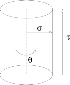
Figure 1: $SL_{2}({\bf R})$ is a solid torus. The upper and lower sides are identified.

Let $Z_{0}$ be a non-compact simply-connected region of $SL_{2}({\bf R})$ consisting of the group elements

$$e^{-\varphi J^{2}}e^{\sigma J^{1}}e^{\psi J^{2}},$$ (2.14)

where $\varphi,\psi$ and $\sigma$ are real parameters. Their ranges are taken $-\infty<\varphi,\psi<+\infty$ and $0<\sigma<+\infty$. $Z_{0}$ is illustrated in Fig.2.

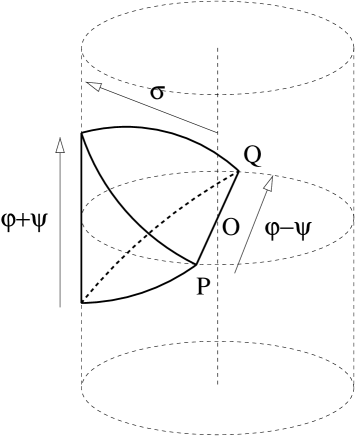
Figure 2: The non-compact simply-connected region $Z_{0}$ of $SL_{2}({\bf R})$

Notice that the line $POQ$ ($\sigma=0$) in Fig.2 is excluded by the definition. The invariant metric (2.6) defines an induced metric on $Z_{0}$. We call it $ds_{0}^{2}$. It is merely a restriction of (2.6) on $Z_{0}$. Regarding the parameters $\varphi,\psi$ and $\sigma$ as coordinates of $Z_{0}$, it can be written in the form

$$ds^{2}_{0}=\frac{l^{2}}{4}\left\{(d\varphi)^{2}+(d\psi)^{2}-(e^{\sigma}+e^{-\sigma})d\varphi d\psi+(d\sigma)^{2}\right\}.$$ (2.15)

We can provide a description of the above region together with the induced metric in terms of $SL_{2}({\bf R})_{+}\times SL_{2}({\bf R})_{-}$ Chern-Simons gravity. To present the description, it is convenient to introduce a mapping,  $SL_{2}({\bf R})_{+}\times SL_{2}({\bf R})_{-}\rightarrow SL_{2}({\bf R})$,  by

$$(g^{(+)},g^{(-)})~{}\longmapsto~{}{g^{(+)}}^{-1}\!g^{(-)}.$$ (2.16)

This defines a pairing of $SL_{2}({\bf R})_{\pm}$ which is invariant under the left diagonal $SL_{2}({\bf R})$ action,  $g^{(\pm)}\mapsto gg^{(\pm)}$. It is also convenient to regard the group elements (2.14) as an image of a function $h$ which takes its values in $SL_{2}({\bf R})$ as presented in (2.14). Explicitly $h$ is given by

$$h(\varphi,\psi,\sigma)\equiv e^{-\varphi J^{2}}e^{\sigma J^{1}}e^{\psi J^{2}}.$$ (2.17)

With this perspective, we can consider the following decomposition of $h$ into a product of $SL_{2}({\bf R})_{\pm}$-valued functions $h^{(\pm)}$ :

$$h={h^{(+)}}^{-1}h^{(-)}.$$ (2.18)

This decomposition is equivalent to construct a pre-image of $Z_{0}$ in the mapping (2.16). It is unique up to the left diagonal $SL_{2}({\bf R})$ gauge transformation. This symmetry turns out to be the three-dimensional local Lorentz symmetry. Given such $SL_{2}({\bf R})_{\pm}$-valued functions, we can associate flat $SL_{2}({\bf R})$ connections $A_{0}^{(\pm)}$ as follows :

$$A_{0}^{(\pm)}\equiv h^{(\pm)}d{h^{(\pm)}}^{-1}.$$ (2.19)

It turns out that $A_{0}\equiv(A_{0}^{(+)},A_{0}^{(-)})$ is a desired classical solution of the Chern-Simons gravity. In fact, one can reproduce the metric (2.15) by means of the 3-vein $e^{a}$ which is obtained from $A_{0}$ through the following correspondence [13, 4] between the relativity and gauge theory languages:

$$A_{0}^{(\pm)}=\pm\frac{1}{l}e+\omega.$$ (2.20)

Both 3-vein $e^{a}$ and spin connection $\omega^{a}$ are realized as $sl_{2}({\bf R})-$valued one-forms,  $e\equiv e^{a}J_{a}$ and $\omega\equiv\omega^{a}J_{a}$. To be explicit, by use of this correspondence, the 3-vein $e$ has the expression $e=\frac{l}{2}(A_{0}^{(+)}-A_{0}^{(-)})$. It can be also expressed as $e=\frac{l}{2}h^{(-)}\cdot{h}^{-1}dh\cdot{h^{(-)}}^{-1}$. Then the metric $e^{a}e_{a}$  $(=2~{}{\rm Tr}~{}e^{2})$  acquires the form, $\frac{l^{2}}{2}{\rm Tr}~{}(h^{-1}dh)^{2}$. This is exactly the induced metric $ds_{0}^{2}$. The correspondence (2.20) also shows that the flatness of the connection $A_{0}$ is equivalent to the Cartan form of the vacuum Einstein equation with the negative cosmological constant

$$de^{a}+\epsilon^{abc}\omega_{b}\wedge e_{c} = 0,$$

$$dw^{a}+\frac{1}{2}\epsilon^{abc}\omega_{b}\wedge\omega_{c}+\frac{1}{2l^{2}}\epsilon^{abc}e_{b}\wedge e_{c} = 0.$$ (2.21)

The non-compact simply-connected region $Z_{0}$ is a covering space of $X_{(J,M)}^{+}$, the exterior of the outer horizon of the non-extremal black hole $X_{(J,M)}$. The projection $\pi$ can be described by using the relations

$$\frac{r_{+}+r_{-}}{l}\left(\frac{t}{l}+\phi\right) = \varphi,$$

$$\frac{r_{+}-r_{-}}{l}\left(\frac{t}{l}-\phi\right) = \psi,$$

$$\frac{\sqrt{r^{2}-r_{+}^{2}}+\sqrt{r^{2}-r_{-}^{2}}}{\sqrt{r_{+}^{2}-r_{-}^{2}}} = e^{\sigma/2},$$ (2.22)

besides the identification of the Schwarzschild angular coordinate, $\phi\sim\phi+2\pi$. See Fig.3.

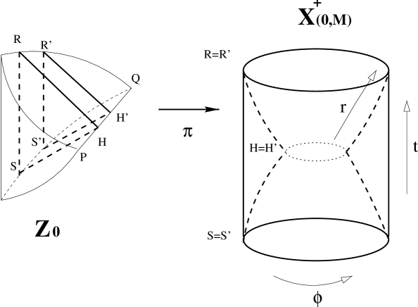
Figure 3: The projection from $Z_{0}$ to the exterior of the outer horizon of the non-extremal black hole. $J=0$ case is depicted as an example. The space between two surfaces $HRS$ and $H^{{}^{\prime}}R^{{}^{\prime}}S^{{}^{\prime}}$ is the fundamental region.

This projection map becomes the isometry : $\pi_{*}ds_{0}^{2}=ds^{2}_{X_{(J,M)}^{+}}$. Therefore the exterior of the outer horizon can be identified with the quotient of $Z_{0}$ :

$$X^{+}_{(J,M)}=Z_{0}/\sim.$$ (2.23)

Here the equivalence relation “$\sim$”, which originates in the periodicity of $\phi$, is given by

$$(\varphi,\psi,\sigma)\sim(\varphi+2\pi\frac{r_{+}+r_{-}}{l},\psi-2\pi\frac{r_{+}-r_{-}}{l},\sigma).$$ (2.24)

It turns out convenient to introduce another parametrization of $Z_{0}$ which is slightly different from $(\varphi,\psi,\sigma)$. Let $b_{0},\tilde{b}_{0}$ and $c$ be the quantities

$$b_{0}\equiv\frac{(r_{+}+r_{-})^{2}}{16Gl},~{}~{}~{}\tilde{b}_{0}\equiv\frac{(r_{+}-r_{-})^{2}}{16Gl},~{}~{}~{}c\equiv\frac{3l}{2G}.$$ (2.25)

We can write any element of $Z_{0}$ in the form

$$e^{-\sqrt{\frac{b_{0}}{c/24}}wJ^{2}}e^{(\rho-\frac{1}{2}\ln\frac{b_{0}\tilde{b}_{0}}{(c/6)^{2}})J^{1}}e^{\sqrt{\frac{\tilde{b}_{0}}{c/24}}\tilde{w}J^{2}},$$ (2.26)

where $w,\tilde{w}$ and $\rho$ are real parameters. To exactly cover $Z_{0}$ with this parametrization, the ranges of $w,\tilde{w}$ and $\rho$ must be taken as $-\infty<w,\tilde{w}<+\infty$ and $\frac{1}{2}\ln\frac{b_{0}\tilde{b}_{0}}{(c/6)^{2}}<\rho<+\infty$.

Using this parametrization or coordinates of $Z_{0}$, let us provide an explicit form of the corresponding classical solution of the Chern-Simons gravity. The $SL_{2}({\bf R})$-valued function $h$, which is defined in (2.17), can be read in this coordinate as

$$h(w,\tilde{w},\rho)=e^{-\sqrt{\frac{b_{0}}{c/24}}wJ^{2}}e^{(\rho-\frac{1}{2}\ln\frac{b_{0}\tilde{b}_{0}}{(c/6)^{2}})J^{1}}e^{\sqrt{\frac{\tilde{b}_{0}}{c/24}}\tilde{w}J^{2}}.$$ (2.27)

The following decomposition of (2.27) may be chosen

$$h^{(+)} = e^{-\frac{1}{2}(\rho-\ln\frac{b_{0}}{c/6})J^{1}}e^{\sqrt{\frac{b_{0}}{c/24}}wJ^{2}},$$

$$h^{(-)} = e^{\frac{1}{2}(\rho-\ln\frac{\tilde{b}_{0}}{c/6})J^{1}}e^{\sqrt{\frac{\tilde{b}_{0}}{c/24}}\tilde{w}J^{2}}.$$ (2.28)

With this choice, the flat connections $A_{0}^{(\pm)}$, which are defined in (2.19), become

$$A_{0}^{(+)}=\left(\begin{array}[]{cc}-\frac{1}{4}d\rho&-e^{\rho/2}dw\\ -\frac{b_{0}}{c/6}e^{-\rho/2}dw&\frac{1}{4}d\rho\end{array}\right),~{}~{}~{}A_{0}^{(-)}=\left(\begin{array}[]{cc}\frac{1}{4}d\rho&-\frac{\tilde{b}_{0}}{c/6}e^{-\rho/2}d\tilde{w}\\ -e^{\rho/2}d\tilde{w}&-\frac{1}{4}d\rho\end{array}\right).$$ (2.33)

Then $A_{0}=(A_{0}^{(+)},A_{0}^{(-)})$ turns out to give the metric

$$ds_{(b_{0},\tilde{b_{0}})}^{2}=l^{2}\left\{\frac{b_{0}}{c/6}(dw)^{2}+\frac{\tilde{b}_{0}}{c/6}(d\tilde{w})^{2}-\left(e^{\rho}+\frac{b_{0}\tilde{b}_{0}}{(c/6)^{2}}e^{-\rho}\right)dwd\tilde{w}+\frac{1}{4}(d\rho)^{2}\right\}.$$ (2.34)

After the change of the coordinates, which can be read from (2.14) and (2.26), it coincides with the induced metric $ds^{2}_{0}$. In terms of the coordinates $(w,\tilde{w},\rho)$, the equivalence relation (2.24) used in the identification with the black hole becomes simple :

$$(w,\tilde{w},\rho)\sim(w+2\pi,\tilde{w}-2\pi,\rho).$$ (2.35)

Therefore we can also say that the quotient of $Z_{0}$ by the identification (2.35), together with the induced metric (2.34), is identified with the exterior of the outer horizon of $X_{(J,M)}$.

2.2 Generalization of flat connection

A generalization of the flat $SL_{2}({\bf R})_{+}\times SL_{2}({\bf R})_{-}$ connection (2.33) is examined [14, 6] to find a realization of the asymptotic Virasoro symmetry [5] in terms of the Chern-Simons gravity. It has the following form

$$A_{b}^{(+)}=\left(\begin{array}[]{cc}-\frac{1}{4}d\rho&-e^{\rho/2}dw\\ -\frac{b(w)}{c/6}e^{-\rho/2}dw&\frac{1}{4}d\rho\end{array}\right),~{}~{}~{}A_{\tilde{b}}^{(-)}=\left(\begin{array}[]{cc}\frac{1}{4}d\rho&-\frac{\tilde{b}(\tilde{w})}{c/6}e^{-\rho/2}d\tilde{w}\\ -e^{\rho/2}d\tilde{w}&-\frac{1}{4}d\rho\end{array}\right).$$ (2.40)

The suffix $b$ and $\tilde{b}$ label the flat connections. To be consistent with the equivalence relation (2.35), we assume that $b$ and $\tilde{b}$ are respectively real functions of $w$ and $\tilde{w}$ with $2\pi$ periodicity.

The asymptotic Virasoro algebra may be realized by the following generators of the infinitesimal gauge transformation

$$\lambda_{f}^{(+)}=\left(\begin{array}[]{cc}-\frac{1}{2}f^{\prime}&fe^{\rho/2}\\ (\frac{b}{c/6}f-\frac{1}{2}f^{\prime\prime})e^{-\rho/2}&\frac{1}{2}f^{\prime}\end{array}\right),~{}~{}~{}\lambda_{\tilde{f}}^{(-)}=\left(\begin{array}[]{cc}\frac{1}{2}\tilde{f}^{\prime}&(\frac{\tilde{b}}{c/6}\tilde{f}-\frac{1}{2}\tilde{f}^{\prime\prime})e^{-\rho/2}\\ \tilde{f}e^{\rho/2}&-\frac{1}{2}\tilde{f}^{\prime}\end{array}\right),$$ (2.45)

where, again to be consistent with (2.35), $f=f(w)$ and $\tilde{f}=\tilde{f}(\tilde{w})$ are assumed to be real functions with $2\pi$ periodicity. The gauge transformation of the connection (2.40) equals [15] to deformations of $b$ and $\tilde{b}$

$$\delta_{\lambda_{f}^{(+)}}A_{b}^{(+)}=\left(\begin{array}[]{cc}0&0\\ -\frac{\delta_{f}b}{c/6}e^{-\rho/2}dw&0\end{array}\right),~{}~{}\delta_{\lambda_{\tilde{f}}^{(-)}}A_{\tilde{b}}^{(-)}=\left(\begin{array}[]{cc}0&-\frac{\delta_{\tilde{f}}\tilde{b}}{c/6}e^{-\rho/2}d\tilde{w}\\ 0&0\end{array}\right).$$ (2.50)

These deformations have the forms

$$\delta_{f}b = fb^{\prime}+2f^{\prime}b-\frac{c}{12}f^{\prime\prime\prime},$$

$$\delta_{\tilde{f}}\tilde{b} = \tilde{f}\tilde{b}^{\prime}+2\tilde{f}^{\prime}\tilde{b}-\frac{c}{12}\tilde{f}^{\prime\prime\prime}.$$ (2.51)

In the asymptotic region where $\rho$ is very large, the non-zero off-diagonal elements of $\delta_{\lambda_{f}^{(+)}}A_{b}^{(+)}$ and $\delta_{\lambda_{\tilde{f}}^{(-)}}A_{\tilde{b}}^{(-)}$ become negligible. Hence the gauge transformation can be regarded as a asymptotic symmetry. To contact with the asymptotic Virasoro symmetry it is convenient to decompose the gauge transformation into the diffeomorphism and the local Lorentz transformation. Notice that, for a given flat connection $A$, its infinitesimal general coordinates transform (say, generated by a vector field $\xi$) can be interpreted [4] as its infinitesimal gauge transform. Via the Sugawara construction the generator of the gauge transformation is given by $\lambda\equiv\xi^{\mu}A_{\mu}$. Decompose the gauge transformation (2.50) to $\delta_{\lambda_{f}^{(+)}}A_{b}^{(+)}$ $=\delta_{\xi}A_{b}^{(+)}+\delta_{\eta}A_{b}^{(+)}$ and $\delta_{\lambda_{\tilde{f}}^{(-)}}A_{\tilde{b}}^{(-)}$ $=\delta_{\tilde{\xi}}A_{\tilde{b}}^{(-)}+\delta_{\eta}A_{\tilde{b}}^{(-)}$, where $\xi,\tilde{\xi}$ are vector fields and $\eta$ is a generator of the local Lorentz transformation (the diagonal $SL_{2}({\bf R})$ gauge transformation). The vector fields turn out to be

$$\xi = 2f^{\prime}\partial_{\rho}+\left(-f+\frac{\frac{\tilde{b}}{c/6}f^{\prime\prime}e^{-\rho}+\tilde{f}^{\prime\prime}}{\frac{b\tilde{b}}{(c/6)^{2}}e^{-\rho}-e^{\rho}}\right)\partial_{w},$$

$$\tilde{\xi} = 2\tilde{f}^{\prime}\partial_{\rho}+\left(-\tilde{f}+\frac{\frac{b}{c/6}\tilde{f}^{\prime\prime}e^{-\rho}+f^{\prime\prime}}{\frac{b\tilde{b}}{(c/6)^{2}}e^{-\rho}-e^{\rho}}\right)\partial_{\tilde{w}}.$$ (2.52)

In the asymptotic region they behave as $\xi$ $\sim 2f^{\prime}\partial_{\rho}-f\partial_{w}$ and $\tilde{\xi}\sim$ $2\tilde{f}^{\prime}\partial_{\rho}-\tilde{f}\partial_{\tilde{w}}$. These coincide with the Virasoro generators considered in [5].

2.3 Generalization of black hole

Given the flat connection (2.40), one can construct a metric according to the prescription of the Chern-Simons gravity. Denote this metric by $ds_{(b,\tilde{b})}^{2}$. It has the form

$$ds^{2}_{(b,\tilde{b})}=l^{2}\left\{\frac{b}{c/6}(dw)^{2}+\frac{\tilde{b}}{c/6}(d\tilde{w})^{2}-\left(e^{\rho}+\frac{b\tilde{b}}{(c/6)^{2}}e^{-\rho}\right)dwd\tilde{w}+\frac{1}{4}(d\rho)^{2}\right\}.$$ (2.53)

It is also possible to obtain a region of $SL_{2}({\bf R})$, analogous to $Z_{0}$, on which the induced metric from $SL_{2}({\bf R})$ is precisely given by (2.53). Since $A_{b}^{(+)}$ and $A_{\tilde{b}}^{(-)}$ are flat connections we can always trivialize them by some $SL_{2}({\bf R})_{\pm}$-valued functions $h_{b}^{(+)}$ and $h_{\tilde{b}}^{(-)}$

$$A_{b}^{(+)}=h_{b}^{(+)}d{h_{b}^{(+)}}^{-1},~{}~{}~{}A_{\tilde{b}}^{(-)}=h_{\tilde{b}}^{(-)}d{h_{\tilde{b}}^{(-)}}^{-1}.$$ (2.54)

Then the desired region of $SL_{2}({\bf R})$, which we will call $Z_{(b,\tilde{b})}$, consists of those obtained from $h_{b}^{(+)}$ and $h_{\tilde{b}}^{(-)}$ by their local Lorentz invariant pairing, ${h_{b}^{(+)}}^{-1}h_{\tilde{b}}^{(-)}$. It is easy to see that the induced metric on $Z_{(b,\tilde{b})}$ is nothing but $ds_{(b,\tilde{b})}^{2}$. When both $b$ and $\tilde{b}$ are constant, $Z_{(b,\tilde{b})}$ coincides with $Z_{0}$. In particular $Z_{(b_{0},\tilde{b}_{0})}=Z_{0}$ holds. On the other hand, as far as $b$ or $\tilde{b}$ is not constant, $Z_{(b,\tilde{b})}$ becomes the region of $SL_{2}({\bf R})$ which is different from $Z_{0}$. One may suspect that a reparametrization of $Z_{0}$ such as $\displaystyle{e^{-\int^{w}\sqrt{\frac{b}{c/24}}dwJ^{2}}e^{(\rho-\frac{1}{2}\ln\frac{b\tilde{b}}{(c/6)^{2}})J^{1}}e^{\int^{\tilde{w}}\sqrt{\frac{\tilde{b}}{c/24}}d\tilde{w}J^{2}}}$ might lead the flat connection (2.40) or the metric (2.53). But it does not so as far as $b$ or $\tilde{b}$ is not constant.

It is an interesting but hard task to describe the region $Z_{(b,\tilde{b})}$ explicitly. Nevertheless, the following argument shows that $Z_{(b.\tilde{b})}$ is generically different from $Z_{0}$ in $SL_{2}({\bf R})$, which is enough for our discussion in this article. We first notice that the completion of $Z_{0}$ at $\sigma=0$ is achived by adding the one-dimensional line $POQ$ (Fig.2) in $SL_{2}({\bf R})$. It is a counterpart of the outer horizon in $SL_{2}({\bf R})$ . This can be read from the induced metric $ds^{2}_{(b_{0},\tilde{b}_{0})}$ of $Z_{0}$. The counterpart of the horizon is located at $\sigma=0$, that is, $\rho=\frac{1}{2}\ln\frac{b_{0}\tilde{b}_{0}}{(c/6)^{2}}$ and there the metric degenerates to

$$\left.ds^{2}_{(b_{0},\tilde{b}_{0})}\right|_{\rho=\frac{1}{2}\ln\frac{b_{0}\tilde{b}_{0}}{(c/6)^{2}}}=l^{2}\left(\sqrt{\frac{b_{0}}{c/6}}dw-\sqrt{\frac{\tilde{b}_{0}}{c/6}}d\tilde{w}\right)^{2}.$$ (2.55)

As regards a generic $Z_{(b,\tilde{b})}$, the analogue of the horizon will be read from the singularity of the vector fields $\xi$ and $\tilde{\xi}$. Looking at (2.52), they diverge at $\rho=\frac{1}{2}\ln\frac{b\tilde{b}}{(c/6)^{2}}$. For the diffeomorphism to work, $\rho$ should satisfy $\rho>\frac{1}{2}\ln\frac{b_{0}\tilde{b}_{0}}{(c/6)^{2}}$. Only with this understanding $Z_{(b,\tilde{b})}$ becomes a deformation of $Z_{0}$. (The vector fields $\xi$ and $\tilde{\xi}$ can be expected to be integrated step by step from $Z_{0}$ to $Z_{(b,\tilde{b})}$ in $SL_{2}({\bf R})$.) The completion of $Z_{(b,\tilde{b})}$ at $\rho=\frac{1}{2}\ln\frac{b_{0}\tilde{b}_{0}}{(c/6)^{2}}$ will be done by adding a two-dimensional space-like surface in $SL_{2}({\bf R})$. This can be also understood from the behavior of the induced metric

$$\left.ds^{2}_{(b,\tilde{b})}\right|_{\rho=\frac{1}{2}\ln\frac{b\tilde{b}}{(c/6)^{2}}}=l^{2}\left(\sqrt{\frac{b}{c/6}}dw-\sqrt{\frac{\tilde{b}}{c/6}}d\tilde{w}\right)^{2}+l^{2}\left(\frac{b^{\prime}}{4b}dw+\frac{\tilde{b}^{\prime}}{4\tilde{b}}d\tilde{w}\right)^{2}.$$ (2.56)

The difference under their completions in $SL_{2}({\bf R})$ clearly shows that $Z_{(b,\tilde{b})}$ is the different region from $Z_{0}$ as far as $b$ or $\tilde{b}$ is not constant.

If one identifies $w$ and $\tilde{w}$ with the coordinates of circles, each deformation $\delta_{f}b$ and $\delta_{\tilde{f}}\tilde{b}$ given in (2.51) can be regarded as the coadjoint action of the Virasoro algebra with the central charge $c$. Here $b$ and $\tilde{b}$ play the role of quadratic differentials on the circles. Let us consider the coadjoint orbits of $b_{0}$ and $\tilde{b}_{0}$ . We will call them respectively $W_{b_{0}}^{(+)}$ and $W_{\tilde{b}_{0}}^{(-)}$. Their product $W_{b_{0}}^{(+)}\times W_{\tilde{b}_{0}}^{(-)}$ may be identified with the family of the regions $Z_{(b,\tilde{b})}$ of $SL_{2}({\bf R})$. Strictly speaking, we should consider not $Z_{(b,\tilde{b})}$ itself but its quotient obtained by the identification $(w,\tilde{w},\rho)\sim(w+2\pi,\tilde{w}-2\pi,\rho)$. This is because the information about $b_{0}$ and $\tilde{b}_{0}$, that is, about mass and angular momentum of the black hole, is encoded not in $Z_{0}$ itself but, through the parametrization (2.26), encoded in the way how to take the quotient. The actions of the Virasoro algebra are consistent with the equivalence relation used in the quotient. Therefore we can discuss about the Virasoro deformation of the quotient space. Let $Y_{(b,\tilde{b})}$ be the quotient $Z_{(b,\tilde{b})}/\sim$. In particular $Y_{(b_{0},\tilde{b}_{0})}$ is identified with $X_{(J,M)}^{+}$, the exterior of the outer horizon of the black hole $X_{(J,M)}$. The Virasoro groups $\widehat{{\it diff}S^{1}}_{+}\times\widehat{{\it diff}S^{1}}_{-}$ deform the metric $ds^{2}_{X_{(J,M)}}=\pi_{*}ds^{2}_{(b_{0},\tilde{b}_{0})}$ of $X_{(J,M)}^{+}$ preserving its asymptotic form. The deformed metric $\pi_{*}ds^{2}_{(b,\tilde{b})}$ is nothing but the metric of $Y_{(b,\tilde{b})}$ which is related with $X_{(J,M)}^{+}$ by the coadjoint action. $SL_{2}({\bf R})$ itself plays the role of a classifying space in this argument. Namely the coadjoint action of $\widehat{{\it diff}S^{1}}_{+}\times\widehat{{\it diff}S^{1}}_{-}$ deforms the region $Z_{0}$ without touching the metric of $SL_{2}({\bf R})$. The metric $ds^{2}_{(b,\tilde{b})}$ of each deformed region $Z_{(b,\tilde{b})}$ is the one induced from $ds^{2}_{SL_{2}({\bf R})}$ and determines the metric of $Y_{(b,\tilde{b})}$ by the projection $\pi$. It is the deformed metric of the black hole.

It should be emphasized that the above Virasoro deformation can not transform the black hole $X^{+}_{(J,M)}$ to the black hole $X^{+}_{(J^{\prime},M^{\prime})}$ which mass $M^{\prime}$ and angular momentum $J^{\prime}$ are different from $M$ and $J$. This can be understood by the fact that any constant shifts of $b_{0}$ and $\tilde{b}_{0}$ are not allowed in (2.51) since $f$ and $\tilde{f}$ are taken to be $2\pi$-periodic for the consistency with the equivalence relation used in the projection $\pi$. What the deformation generates are the oscillating modes of $b(w)$ and $\tilde{b}(\tilde{w})$. The deformed metric $\pi_{*}ds^{2}_{(b,\tilde{b})}$ is not static since $w$ and $\tilde{w}$ are originally the light cone coordinates (2.22).

3 3-Geometries As The Virasoro Coadjoint Orbit

3.1 Coadjoint orbits of the Virasoro group

The Virasoro algebra is the Lie algebra of the Virasoro group $\widehat{{\it diff}S^{1}}$, which is the central extension of ${\it diff}S^{1}$, the group of diffeomorphisms of a circle. It consists of vector fields $f(w)\frac{d}{dw}$ on the circle together with a central element $c$. A general element has the form $f(w)\frac{d}{dw}-iac$ with $a$ a real number. Let us write it by the pair $(f,a)$. The commutation relation is given by

$$\left[(f,a_{1}),(g,a_{2})\right]=\left(fg^{\prime}-f^{\prime}g,~{}\frac{1}{48\pi}\!\int_{0}^{2\pi}\!dw(fg^{\prime\prime\prime}-f^{\prime\prime\prime}g)\right).$$ (3.1)

The coadjoint representation of the Virasoro algebra consists of quadratic differentials $b(w)(dw)^{2}$ together with the dual central element $c^{*}$. A general coadjoint vector (an element of the dual of the Virasoro algebra) has the form $b(w)(dw)^{2}+itc^{*}$ with $t$ a real number. Let us denote it by the pair $(b,t)$. The pairing between coadjoint and adjoint vectors are given by

$$\langle(b,t),(g,a)\rangle=\frac{1}{2\pi}\int_{0}^{2\pi}dwb(w)g(w)~{}~{}+ta.$$ (3.2)

This is invariant under reparametrizations of the circle. The coadjoint action of the Virasoro algebra is

$$\delta_{f}(b,t)=(fb^{\prime}+2f^{\prime}b-\frac{t}{12}f^{\prime\prime\prime},0),$$ (3.3)

where, the action of the central element being trivial, we write $\delta_{(f,a)}$ as $\delta_{f}$ for short. The dual pairing (3.2) is invariant under the action of the Virasoro algebra,

$$\delta_{f}\langle(b,t),(g,a)\rangle = \langle\delta_{f}(b,t),(g,a)\rangle+\langle(b,t),\delta_{f}(g,a)\rangle$$ (3.4)

$$= 0,$$

where $\delta_{f}(g,a)$ is given by (3.1).

As can be seen in (3.3) the dual central element $c^{*}$ is invariant under the coadjoint action. The value of $t$ determines the central charge. We shall set $t=\frac{3l}{2G}$. According to the definition (2.25) we will write this $t$ as $c$. And $W_{b_{0}}$, written as $W_{b_{0},\tilde{b}_{0}}^{(\pm)}$ at the end of the previous section, is the coadjoint orbit of $(b_{0},c)$, that is, the $\widehat{{\it diff}S^{1}}$-orbit of $(b_{0},c)$. The transformation (3.3) also shows that $W_{b_{0}}$ is a homogeneous space of ${\it diff}S^{1}$. Therefore we can parametrize the orbit by elements of ${\it diff}S^{1}$ ( modulo the little group $H$ ) : For $s\in{\it diff}S^{1}$, letting $w_{s}=s(w)$, the integrated form of (2.51) or (3.3) becomes

$$b^{s}(w_{s})(dw_{s})^{2}=\left[b_{0}+\frac{c}{12}\{w_{s},w\}\right](dw)^{2},$$ (3.5)

where $\{w_{s},w\}$ is the Schwarzian derivative, $\{w_{s},w\}\equiv$ $\frac{d^{3}w_{s}/dw^{3}}{dw_{s}/dw}$ $-\frac{3}{2}\left(\frac{d^{2}w_{s}/dw^{2}}{dw_{s}/dw}\right)^{2}$. Then $b^{s}$ provides the corresponding element of $W_{b_{0}}$.

According to the Kirillov-Souriau-Kostant theory [16], each coadjoint orbit admits to have a canonical symplectic structure defined by the dual pairing. If one regards tangent vectors at $b^{s}$ as vector fields on the circle, the symplectic form $\Omega$ can be described as follows :

$$\Omega|_{b^{s}}(u,v)=\langle(b^{s},c),\left[(u,0),(v,0)\right]\rangle,$$ (3.6)

where $u=u(w_{s}),v=v(w_{s})$ denote tangent vectors at $b^{s}$.

Generators of the Virasoro algebra are given by Hamiltonian functions on $W_{b_{0}}$. If one takes $L_{m}=ie^{imw}\frac{d}{dw}$, the commutation relation (3.1) becomes

$$\left[L_{m},L_{n}\right]=(m-n)L_{m+n}+\frac{c}{12}m^{3}\delta_{m+n,0}.$$ (3.7)

The corresponding Hamiltonian functions are given by

$$l_{m}(s)=\langle(b^{s},c),(e^{imw_{s}},0)\rangle,$$ (3.8)

where $s\in{\it diff}S^{1}$ is thought as the coordinate of $W_{b_{0}}$. Using the prescribed symplectic structure [16] they turn out to satisfy the (classical) Virasoro algebra :

$$\{l_{m},l_{n}\}=i(m-n)l_{m+n}+i\frac{c}{12}m^{3}\delta_{m+n,0}.$$ (3.9)

3.2 3-geometries as the Virasoro coadjoint orbit

We generalize our argument given in the previous section to the cases of the massive-extremal and massless black holes. For each of them there appears an appropriate region $Z_{0}$ of $SL_{2}({\bf R})$. The Virasoro groups $\widehat{{\it diff}S^{1}}_{+}\times\widehat{{\it diff}S^{1}}_{-}$ can deform each $Z_{0}$ in $SL_{2}({\bf R})$. This will be described by the coadjoint action of the Virasoro group. Quotient of the deformed region, obtained in a similar manner as the non-extremal case, provides a deformation of the exterior of the outer horizon. Each quotient has a metric induced from $SL_{2}({\bf R})$, which is nothing but the deformed metric of the black hole considered in [6]. The family of these quotients will be identified with the product of the coadjoint orbits $W_{b_{0}}^{(+)}\times W_{\tilde{b}_{0}}^{(-)}$. The values of $b_{0}$ and $\tilde{b}_{0}$ can be read from the values $(J,M)$ of the black hole by using (2.25). We also examine the case of $AdS_{3}$. In this case it becomes necessary to study $\widetilde{SL_{2}}({\bf R})$, the universal cover of $SL_{2}({\bf R})$. Taking an appropriate region of $\widetilde{SL_{2}}(\bf R)$, it becomes possible to repeat an argument similar to the black holes. In particular the family of the deformed regions will be identified with $W_{-c/24}^{(+)}\times W_{-c/24}^{(-)}$.

3.2.1 Extremal black hole

Massive case
Let $Z_{0}$ be a region of $SL_{2}({\bf R})$ consisting of the group elements

$$e^{-\varphi J^{2}}e^{\sigma J^{1}}e^{\tilde{w}J^{-}},$$ (3.10)

where $\varphi,\tilde{w}$ and $\sigma$ are real parameters. There ranges are taken $-\infty<\varphi,\tilde{w},\sigma<+\infty$. It is a non-compact simply-connected region of $SL_{2}({\bf R})$. Regarding these parameters as coordinates of $Z_{0}$, the induced metric from $SL_{2}({\bf R})$ can be written in the form

$$ds^{2}_{0}=\frac{l^{2}}{4}\left\{(d\varphi)^{2}-2e^{\sigma}d\varphi d\tilde{w}+(d\sigma)^{2}\right\}.$$ (3.11)

This non-compact simply-connected region of $SL_{2}({\bf R})$ is a covering space of $X_{(Ml,M)}^{+}$, the exterior of the outer horizon of the massive extremal black hole $X_{(Ml,M)}$. The projection $\pi$ can be described by

$$\frac{2r_{+}}{l}\left(\frac{t}{l}+\phi\right)=\varphi,~{}~{}~{}\frac{t}{l}-\phi=\tilde{w},~{}~{}~{}\frac{r^{2}-r_{+}^{2}}{r_{+}l}=e^{\sigma},$$ (3.12)

with the identification $\phi\sim\phi+2\pi$. Since $\pi$ turns out to be the isometry, we can identify $X_{(Ml,M)}^{+}$ with the quotient of $Z_{0}$ :

$$X^{+}_{(Ml,M)}=Z_{0}/\sim.$$ (3.13)

Here the equivalence relation is given by $(\varphi,\tilde{w},\sigma)\sim$ $(\varphi+4\pi\frac{r_{+}}{l},\tilde{w}-2\pi,\sigma)$.

Reparametrization of the group elements (3.10) to the form

$$e^{-\sqrt{16GM}wJ^{2}}e^{(\rho-\frac{1}{2}\ln 4GM)J^{1}}e^{\tilde{w}J^{-}}~{}~{}~{}~{}~{}~{}(\equiv h(w,\tilde{w},\rho)),$$ (3.14)

leads the flat $SL_{2}({\bf R})_{+}\times SL_{2}({\bf R})_{-}$ connection

$$A_{0}^{(+)}=\left(\begin{array}[]{cc}-\frac{1}{4}d\rho&-e^{\rho/2}dw\\ -4GMe^{-\rho/2}dw&\frac{1}{4}d\rho\end{array}\right),~{}~{}~{}A_{0}^{(-)}=\left(\begin{array}[]{cc}\frac{1}{4}d\rho&0\\ -e^{\rho/2}d\tilde{w}&-\frac{1}{4}d\rho\end{array}\right).$$ (3.19)

In this derivation we first decompose the $SL_{2}({\bf R})$-valued function $h$ (3.14), according to the rule (2.18), into the pair of $SL_{2}({\bf R})_{\pm}$-valued functions, $h^{(+)}=e^{-\frac{1}{2}(\rho-\ln 4GM)J^{1}}e^{\sqrt{16GM}wJ^{2}}$ and $h^{(-)}=e^{\frac{1}{2}\rho J^{1}}e^{\tilde{w}J^{-}}$, and then apply the prescription (2.19). The connection (3.19) coincides with (2.40) at $(b,\tilde{b})=(Ml,0)$.

The equivalence relation used in the quotient (3.13) acquires the form (2.24) in these new coordinates. So our argument completely reduces to that given in the previous section. In particular deformations of the massive-extremal black hole $X_{(Ml,M)}^{+}$ are realized by the quotients $Y_{(b,\tilde{b})}$ which are connected with it by the Virasoro group. The family of these $Y_{(b,\tilde{b})}$ can be identified with $W_{Ml}^{(+)}\times W_{0}^{(-)}$.

Massless case
Let $Z_{0}$ be a region of $SL_{2}({\bf R})$ consisting of the group elements

$$e^{-wJ^{+}}e^{\rho J^{1}}e^{\tilde{w}J^{-}}~{}~{}~{}~{}~{}(\equiv h(w,\tilde{w},\rho)),$$ (3.20)

where $w,\tilde{w}$ and $\rho$ are real parameters. Their ranges are taken $-\infty<w,\tilde{w},\rho<+\infty$. It is also a non-compact simply-connected region of $SL_{2}({\bf R})$. Regarding these parameters as coordinates of $Z_{0}$, the induced metric from $SL_{2}({\bf R})$ can be written as

$$ds^{2}_{0}=\frac{l^{2}}{4}\left\{-4e^{\rho}dwd\tilde{w}+(d\rho)^{2}\right\}.$$ (3.21)

This non-compact simply-connected region is a covering space of $X_{(0,0)}^{+}$, the exterior of the horizon of the massless black hole. The projection $\pi$ is prescribed by

$$\frac{t}{l}+\phi=w,~{}~{}~{}\frac{t}{l}-\phi=\tilde{w},~{}~{}~{}\frac{r}{l}=e^{\rho/2},$$ (3.22)

with the identification $\phi\sim\phi+2\pi$. Hence the exterior of the horizon of the massless black hole can be identified with the quotient of $Z_{0}$ :

$$X^{+}_{(0,0)}=Z_{0}/\sim,$$ (3.23)

where the equivalence relation is $(w,\tilde{w},\rho)\sim$ $(w+2\pi,\tilde{w}-2\pi,\rho)$.

Decomposition of (3.20) by $h^{(+)}=e^{-\frac{1}{2}\rho J^{1}}e^{wJ^{+}}$ and $h^{(-)}=e^{\frac{1}{2}\rho J^{1}}e^{\tilde{w}J^{-}}$ leads the flat $SL_{2}({\bf R})_{+}\times SL_{2}({\bf R})_{-}$ connection

$$A_{0}^{(+)}=\left(\begin{array}[]{cc}-\frac{1}{4}d\rho&-e^{\rho/2}dw\\ 0&\frac{1}{4}d\rho\end{array}\right),~{}~{}~{}A_{0}^{(-)}=\left(\begin{array}[]{cc}\frac{1}{4}d\rho&0\\ -e^{\rho/2}d\tilde{w}&-\frac{1}{4}d\rho\end{array}\right).$$ (3.28)

This is the connection (2.40) at $(b,\tilde{b})=(0,0)$. So our argument also reduces to the previous one. Deformations of the massless black hole $X_{(0,0)}^{+}$ are realized by the quotients $Y_{(b,\tilde{b})}$ which are connected with it by the Virasoro group. The family of these $Y_{(b,\tilde{b})}$ can be identified with $W_{0}^{(+)}\times W_{0}^{(-)}$.

3.2.2 Anti de-Sitter space

$AdS_{3}$ is the universal cover of $SL_{2}({\bf R})$. In terms of the Schwarzschild type coordinates $(t,\phi,r)$, where the ranges are $-\infty<t<+\infty$, $0\leq\phi<2\pi$ and $0\leq r<+\infty$, the metric $ds_{AdS_{3}}^{2}$ acquires the form

$$ds_{AdS_{3}}^{2}=-\left(1+\frac{r^{2}}{l^{2}}\right)^{2}(dt)^{2}+\left(1+\frac{r^{2}}{l^{2}}\right)^{-2}(dr)^{2}+r^{2}(d\phi)^{2}.$$ (3.29)

Notice that $r=0$ is not a true singularity. It is merely a coordinate singularity. Nevertheless, to provide the Virasoro deformation of this space which is analogous to the black holes, it is required to consider the complement of $r=0$ rather than the whole. Actually this complement is an analogue of $X_{(J,M)}^{+}$ of the black hole. The complement of the line at $r=0$ will be called $AdS_{3}^{+}$.

Let $Z_{0}$ be a region of $SL_{2}({\bf R})$ consisting of the group elements

$$e^{-wJ^{0}}e^{\sigma J^{1}}e^{-\tilde{w}J^{0}},$$ (3.30)

where $w,\tilde{w}$ and $\sigma$ are real parameters. Notice that (3.30) have the form of the Cartan decomposition. In order to avoid a doubly parametrization, the ranges of $w$ and $\tilde{w}$ should be taken within $0\leq w\pm\tilde{w}<4\pi$. So we choose $0\leq w\pm\tilde{w}<4\pi$ for their ranges. As regards $\sigma$ it is set to $0<\sigma<+\infty$. If one admits $\sigma=0$ in the definition, $Z_{0}$ coincides with $SL_{2}({\bf R})$ itself. Due to its exclusion $Z_{0}$ becomes the complement of the circle at $\sigma=0$. If one regards the time of $AdS_{3}$ being $2\pi l$-periodic, $Z_{0}$ can be identified with $AdS_{3}^{+}$. The relation with the Schwarzschild type coordinates can be read as

$$w=\frac{t}{l}+\phi,~{}~{}~{}\tilde{w}=\frac{t}{l}-\phi,~{}~{}~{}e^{\sigma/2}=\sqrt{1+\frac{r^{2}}{l^{2}}}+\frac{r}{l}.$$ (3.31)

Introduce a slightly different parametrization of $Z_{0}$ with the form

$$e^{-wJ^{0}}e^{(\rho+2\ln 2)J^{1}}e^{-\tilde{w}J^{0}}~{}~{}~{}~{}~{}(\equiv h(w,\tilde{w},\rho)),$$ (3.32)

where real parameter $\rho$ satisfies $-2\ln 2<\rho<+\infty$, due to the shift. Decomposition of the $SL_{2}({\bf R})$-valued function $h$ (3.32) by the pair of $SL_{2}({\bf R})_{\pm}$-valued functions, $h^{(+)}=e^{-\frac{1}{2}(\rho+2\ln 2)J^{1}}e^{wJ^{0}}$ and $h^{(-)}=e^{\frac{1}{2}(\rho+2\ln 2)J^{1}}e^{-\tilde{w}J^{0}}$ leads the flat $SL_{2}({\bf R})_{+}\times SL_{2}({\bf R})_{-}$ connection

$$A_{0}^{(+)}=\left(\begin{array}[]{cc}-\frac{1}{4}d\rho&-e^{\rho/2}dw\\ \frac{1}{4}e^{-\rho/2}dw&\frac{1}{4}d\rho\end{array}\right),~{}~{}~{}A_{0}^{(-)}=\left(\begin{array}[]{cc}\frac{1}{4}d\rho&\frac{1}{4}e^{-\rho/2}d\tilde{w}\\ -e^{\rho/2}d\tilde{w}&-\frac{1}{4}d\rho\end{array}\right).$$ (3.37)

This is the connection (2.40) at $(b,\tilde{b})=(-c/24,-c/24)$.

$SL_{2}({\bf R})$ has a topologically nontrivial circle. The universal cover $\widetilde{SL_{2}}({\bf R})$ can be obtained by making this $S^{1}$ to a line. This is equivalent to a simple change of the identification of $w$ and $\tilde{w}$ in the Cartan decomposition into an identification, $(w,\tilde{w})\sim(w+2\pi,\tilde{w}-2\pi)$. The universal covering of $Z_{0}$ taken in $\widetilde{SL_{2}}({\bf R})$ is the complement of the line at $\sigma=0$ and can be identified with $AdS_{3}^{+}$.

For a given element $(b,\tilde{b})$ $\in W_{-c/24}^{(+)}\times W_{-c/24}^{(-)}$, the flat connection (2.40) may be thought as a connection on a solid cylinder, where $\rho$ measures its radial direction and $(w,\tilde{w})$ are identified with the lightcone coordinates of the cylinder. Trivializations of $A^{(\pm)}_{b,\tilde{b}}$ and their local Lorentz invariant pairing define a map from the solid cylinder to $SL_{2}({\bf R})$. The solid cylinder wraps $SL_{2}({\bf R})$ infinitely many times. We may unfold this wrapping by considering $\widetilde{SL_{2}}({\bf R})$ in stead of $SL_{2}({\bf R})$. Therefore, letting $Z_{0}$ be the complement of the line in $\widetilde{SL_{2}}({\bf R})$ we can construct its deformation by the Virasoro group. The family of the deformations can be identified with $W_{-c/24}^{(+)}\times W_{-c/24}^{(-)}$.

3.3 Quantization of the Virasoro coadjoint orbits

For a given coadjoint orbit $W_{b_{0}}$, the Hamiltonian function $l_{0}(s)$ generates the $S^{1}$-action and can be considered as an energy function of the orbit. $b_{0}$ is a fixed point of this circle action and corresponds to the classical vacuum. We will discuss about the stability of this vacuum. Write $s\in\widehat{{\it diff}S^{1}}$ in the form $s(w)=w+\sum_{n}s_{n}e^{-inw}$, where $s_{n}$ are complex numbers satisfying $\bar{s}_{n}=s_{-n}$. These $s_{n}$ with $n\neq 0$ provide local coordinates in the neighborhood of $b_{0}$. $s_{0}$ acts trivially on $b_{0}$ (cf.(3.3)). The behavior of the energy function in the neighborhood of $b_{0}$ can be seen by inserting the above $s$ into (3.8) and expanding it with respect to $s_{n}$. The expansion turns out [17] to be the form

$$l_{0}(s)=b_{0}+\sum_{n}n^{2}(b_{0}+\frac{c}{24}n^{2})|s_{n}|^{2}+O(s_{n}^{3}).$$ (3.38)

The stability of the classical vacuum will be assured by the condition, $l_{0}$ being bounded from below at $b_{0}$. It is achieved only when $b_{0}$ satisfies

$$b_{0}\geq-\frac{c}{24}.$$ (3.39)

All the coadjoint orbits corresponding to the 3-geometries under consideration are satisfying this stability condition.

The orbit $W_{b_{0}}$ which satisfies the condition (3.39) can be quantized. This provides a unitary irreducible representation of the Virasoro algebra. Actually it is quantized [18, 19, 17] by the Kähler quantization or geometric quantization method. The coadjoint orbit is topologically the homogeneous space ${\it diff}S^{1}/H$. The little group $H$ is $S^{1}$ for the black holes, and $SL_{2}(\bf{R})$ for $AdS_{3}$ . For these $H$, the homogeneous space ${\it diff}S^{1}/H$ becomes a complex manifold. The complex structure turns out [17] to be compatible with the symplectic structure (3.6). Thereby the orbit $W_{b_{0}}$ which we need, becomes Kähler. The complex line bundle on the orbit with its $1$st Chern class $\Omega$ provides the unitary irreducible representation on the space of the holomorphic sections.

To describe the representations it is convenient to shift the Virasoro generator $L_{0}$ to $L_{0}+\frac{c}{24}$. With this shift the algebra (3.7) becomes the standard form

$$\left[L_{m},L_{n}\right]=(m-n)L_{m+n}+\frac{c}{12}(m^{3}-m)\delta_{m+n,0}.$$ (3.40)

Any representation of the Virasoro algebra with the central charge $c$ can be specified by its highest weight state $|h\rangle$. The state $|h\rangle$, which is called primary, satisfies $L_{0}|h\rangle=h|h\rangle$ and $L_{n}|h\rangle=0$ for $\forall n\geq 1$. In addition to these conditions the primary state $|0\rangle$ satisfies $L_{-1}|0\rangle=0$. So it is a $SL_{2}({\bf R})$ invariant state.

Unitary representations are the representations in which $L_{n}$ satisfy the condition $L_{n}^{\dagger}=L_{-n}$. The unitary irreducible representations which are obtained by the quantization of the orbits can be summarized as follows [17] : For the orbit of $W_{b_{0}}$ with $b_{0}>-c/24$, the corresponding unitary irreducible representation is given by the Verma module ${\cal V}_{h=b_{0}+\frac{c}{24}}$. It is a module obtained by successive actions of $L_{-n}$ ($n\geq 1$) on $|b_{0}+\frac{c}{24}\rangle$. It has the form

$${\cal V}_{b_{0}+\frac{c}{24}}=\bigoplus_{n_{1}\geq n_{2}\geq\cdots\geq n_{k}\geq 1}{\bf C}L_{-n_{1}}L_{-n_{2}}\cdots L_{-n_{k}}|b_{0}+\frac{c}{24}\rangle.$$ (3.41)

For the orbit $W_{-c/24}$, the corresponding unitary irreducible representation is given by an analogue of the Verma module ${\cal V}_{0}$. It is obtained by successive actions of $L_{-n}$ ($n\geq 2$) on $|0\rangle$. We call this module ${\cal V}^{\prime}_{0}$. It has the form

$${\cal V}^{\prime}_{0}=\bigoplus_{n_{1}\geq n_{2}\geq\cdots\geq n_{k}\geq 2}{\bf C}L_{-n_{1}}L_{-n_{2}}\cdots L_{-n_{k}}|0\rangle.$$ (3.42)

Gathering these results about quantization of the orbits we can prescribe quantization of the asymptotic Virasoro symmetry of the 3-geometries or their Virasoro deformations in the following manner : For the BTZ black hole $X_{(J,M)}$, the deformations $Y_{(b,\tilde{b})}$ of the exterior of the outer horizon can be identified with the product of the coadjoint orbits $W_{b_{0}}^{(+)}\times W_{\tilde{b}_{0}}^{(-)}$. The quantizations of the orbits $W_{b_{0}}^{(+)}$ and $W_{\tilde{b}_{0}}^{(-)}$ provide the unitary irreducible representations ${\cal V}^{(+)}_{b_{0}+\frac{c}{24}}$ and ${\cal V}^{(-)}_{b_{0}+\frac{c}{24}}$. Therefore the quantization of the deformations leads the representation ${\cal V}^{(+)}_{b_{0}+\frac{c}{24}}\times{\cal V}^{(-)}_{\tilde{b}_{0}+\frac{c}{24}}$. In particular state of the black hole can be identified with the primary state $|b_{0}+\frac{c}{24}\rangle\otimes$ $|\tilde{b}_{0}+\frac{c}{24}\rangle$ of the representation . For $AdS_{3}$, the deformations of $AdS_{3}^{+}$ can be identified with the product of the coadjoint orbits $W_{-\frac{c}{24}}^{(+)}\times W_{-\frac{c}{24}}^{(-)}$. These orbits provide the unitary irreducible representations ${{\cal V}^{\prime}_{0}}^{(+)}$ and ${{\cal V}^{\prime}_{0}}^{(-)}$. Therefore the quantization of the deformation leads the representation ${{\cal V}^{\prime}_{0}}^{(+)}\times{{\cal V}^{\prime}_{0}}^{(-)}$. The state of $AdS_{3}$ can be identified with the primary state $|0\rangle\otimes$ $|0\rangle$. It is the state invariant under $SL_{2}({\bf R})_{+}\times SL_{2}({\bf R})_{-}$, which is the isometry of $AdS_{3}$.

Excitations by $L_{-n}$ correspond to the Virasoro deformation of $Y_{(b_{0},\tilde{b}_{0})}=Z_{0}/\sim$. Originally it is the deformation of $Z_{0}$ in $SL_{2}({\bf R})$ which by no means provides any transformation of the black hole to another one having different mass and angular momentum . Nevertheless, these degrees of freedom provide the unitary representations of the Virasoro algebra. This shows that these degrees of freedom can be included in the physical spectrum as (massive) gravitons [20].

4 Quantization Of Three-Dimensional Gravity

As we have seen, quantizations of the Virasoro deformations of the BTZ black holes and $AdS_{3}$ lead the unitary irreducible representations of the Virasoro algebra at least when $\frac{3l}{2G}\geq 1$. One may wonder quantization of three-dimensional gravity with negative cosmological constant becomes complete by these quantizations. But it does not so. If one takes the Chern-Simons gravity viewpoint, these deformations correspond to the local degrees of freedom of the theory (gravitons), that is, oscillating modes of $b$ and $\tilde{b}$ in the flat connection (2.40). To make the quantization complete, one must take into account of the global degrees of freedom, i.e., holonomies. The holonomy variables should be dynamical in the Chern-Simons gauge theory. In our context this requires an introduction of their conjugates. Given a suitable Poisson structure on the holonomy variables and their quantizations, it is very reasonable to expect from the perspective of the $AdS_{3}/CFT_{2}$ correspondence that, with an identification of these quantum operators with the zero modes of an appropriate two-dimensional quantum field, the unitary representations obtained in the previous section could be reproduced as the Hilbert space of the two-dimensional conformal field theory. This expectation turns out to be true at least when $\frac{3l}{2G}\gg 1$. The holonomy variables can be identified with the zero modes of a real scalar field $X$. This scalar field should be interpreted as the Liouville field in the ultimate.

We start with the description of the Poisson structure of the holonomies. Then we turn to construction of the unitary irreducible representations in the framework of the Liouville field theory or the Coulomb gas formalism. Finally we make identifications between the states of the three-dimensional gravity and those of the Liouville field theory.

4.1 Holonomy variable

For a given closed path $\gamma$, holonomy of a connection $A=(A^{(+)},A^{(-)})$ along the path is given by

$$H^{(\pm)}[\gamma]\equiv Pe^{\int_{\gamma}A^{(\pm)}},$$ (4.1)

where $P$ denotes the path ordering. Since we can assume $A$ is flat, $H[\gamma]=(H^{(+)}[\gamma],H^{(-)}[\gamma])$ is invariant up to conjugation under smooth deformations of $\gamma$. In particular ${\rm Tr}H^{(\pm)}$ are homotopy invariant. The BTZ black holes originally admit to have a nontrivial holonomy around a closed path connecting $(w,\tilde{w},\rho)$ and $(w+2\pi,\tilde{w}-2\pi,\rho)$ in the constant $\rho$ surface. Let us call this path $\gamma_{1}$. If there is only one nontrivial holonomy there appears no symplectic structure. In order to make it a dynamical variable we need to introduce another “closed” path. Let $\gamma_{2}$ be a path connecting $(w,\tilde{w},\rho)$ and $(w+\sqrt{\frac{c/6}{b_{0}}}\Sigma,\tilde{w}+\sqrt{\frac{c/6}{\tilde{b}_{0}}}\tilde{\Sigma},\rho)$ in the constant $\rho$ surface. If one regards it as a closed path and then considers about a holonomy around this path, the quantities $\Sigma$ and $\tilde{\Sigma}$ together with $r_{\pm}$ may become dynamical. In this extended “phase” space, the BTZ black holes themselves will become a Lagrangian submanifold $\Sigma=\tilde{\Sigma}=0$. This extension is a generalization of the off-shell extension of the Euclidean black holes examined by Carlip and Teitelboim [21].

The flat connection which describes $X^{+}_{(J,M)}$, the exterior of the outer horizon of the non-extremal BTZ black hole, is given by (2.33). The holonomy of this connection around the path $\gamma_{1}$ can be evaluated as

$$H^{(+)}[\gamma_{1}] = h^{(+)}(w+2\pi,\tilde{w}-2\pi,\rho){h^{(+)}}^{-1}(w,\tilde{w},\rho)$$

$$= e^{-\frac{1}{2}(\rho-\ln\frac{b_{0}}{c/6})J^{1}}e^{2\pi\sqrt{\frac{b_{0}}{c/24}}J^{2}}e^{\frac{1}{2}(\rho-\ln\frac{b_{0}}{c/6})J^{1}},$$

$$H^{(-)}[\gamma_{1}] = h^{(-)}(w+2\pi,\tilde{w}-2\pi,\rho){h^{(-)}}^{-1}(w,\tilde{w},\rho)$$ (4.2)

$$= e^{\frac{1}{2}(\rho-\ln\frac{\tilde{b}_{0}}{c/6})J^{1}}e^{-2\pi\sqrt{\frac{\tilde{b}_{0}}{c/24}}J^{2}}e^{-\frac{1}{2}(\rho-\ln\frac{\tilde{b}_{0}}{c/6})J^{1}},$$

where $h^{(\pm)}$ are those used in its trivialization and their explicit forms are given in (2.28). The trace becomes

$${\rm Tr}H^{(+)}[\gamma_{1}]=2\cosh\pi\sqrt{\frac{b_{0}}{c/24}},~{}~{}~{}{\rm Tr}H^{(-)}[\gamma_{1}]=2\cosh\pi\sqrt{\frac{\tilde{b}_{0}}{c/24}}.$$ (4.3)

Similarly its holonomy around the path $\gamma_{2}$ has the form

$$H^{(+)}[\gamma_{2}] = e^{-\frac{1}{2}(\rho-\ln\frac{b_{0}}{c/6})J^{1}}e^{2\Sigma J^{2}}e^{\frac{1}{2}(\rho-\ln\frac{b_{0}}{c/6})J^{1}},$$

$$H^{(-)}[\gamma_{2}] = e^{\frac{1}{2}(\rho-\ln\frac{\tilde{b}_{0}}{c/6})J^{1}}e^{2\tilde{\Sigma}J^{2}}e^{-\frac{1}{2}(\rho-\ln\frac{\tilde{b}_{0}}{c/6})J^{1}}.$$ (4.4)

Therefore we obtain

$${\rm Tr}H^{(+)}[\gamma_{2}]=2\cosh\Sigma,~{}~{}~{}{\rm Tr}H^{(-)}[\gamma_{2}]=2\cosh\tilde{\Sigma}.$$ (4.5)

To describe the Poisson structure of these holonomies in the Chern-Simons gravity, we follow the recipe developed by Nelson, Regge and Zertuche [22]. It states that holonomies in a constant time surface have non-vanishing Poisson brackets when the underlying paths intersect with each other. If one regards the radial coordinate $\rho$ as a time, the following Poisson algebra of $\mbox{Tr}H^{(\pm)}[\gamma_{i}](i=1,2)$ can be obtained :

$$\left\{{\rm Tr}H^{(\pm)}[\gamma_{1}],{\rm Tr}H^{(\pm)}[\gamma_{2}]\right\}=\mp\frac{6\pi}{c}\left[-\left({\rm Tr}H^{(\pm)}[\gamma_{1}]\right)\left({\rm Tr}H^{(\pm)}[\gamma_{2}]\right)+2{\rm Tr}H^{(\pm)}[\gamma_{2}\gamma_{1}]\right].$$ (4.6)

Substitution of the explicit forms (4.3) and (4.5) simplifies the expression (4.6) to

$$\left\{\cosh\pi\frac{r_{+}+r_{-}}{l},\cosh\Sigma\right\} = -\frac{4\pi G}{l}\sinh\pi\frac{r_{+}+r_{-}}{l}\sinh\Sigma,$$

$$\left\{\cosh\pi\frac{r_{+}-r_{-}}{l},\cosh\tilde{\Sigma}\right\} = -\frac{4\pi G}{l}\sinh\pi\frac{r_{+}-r_{-}}{l}\sinh\tilde{\Sigma}.$$ (4.7)

These indicate that $r_{+},r_{-},\Sigma$ and $\tilde{\Sigma}$ become canonical variables with the Poisson algebra,

$$\left\{r_{+}+r_{-},\Sigma\right\}=-4G,~{}~{}~{}\left\{r_{+}-r_{-},\tilde{\Sigma}\right\}=-4G.$$ (4.8)

Having obtained the symplectic structure, one can quantize these variables. Let $\hat{r}_{+},\hat{r}_{-},\hat{\Sigma}$ and $\hat{\tilde{\Sigma}}$ be the corresponding operators. Their nontrivial commutation relations are

$$\Big{[}\hat{r}_{+}+\hat{r}_{-},\hat{\Sigma}\Big{]}=-4iG,~{}~{}~{}~{}\Big{[}\hat{r}_{+}-\hat{r}_{-},\hat{\tilde{\Sigma}}\Big{]}=-4iG.$$ (4.9)

4.2 Realization by the Liouville field theory

Let $X$ be a real scalar field on ${\bf P}^{1}$. The action is given by

$$S[X]=\frac{1}{4\pi i}\int_{{\bf P}^{1}}\bar{\partial}X\wedge\partial X+\frac{\alpha_{0}}{2\pi}\int_{{\bf P}^{1}}RX,$$ (4.10)

where $R$ is the Riemann tensor of a fixed Kähler metric on ${\bf P}^{1}$. $\alpha_{0}$ is a real number and its value will be specified later.

If one takes the following expansion of $X$ at $z=0$

$$X(z)=x-ip\ln z+i\sum_{n\neq 0}\frac{a_{n}}{n}z^{-n},$$ (4.11)

the nontrivial commutation relations among the mode operators become

$$\left[x,p\right]=i,~{}~{}~{}\left[a_{m},a_{n}\right]=m\delta_{m+n,0},$$ (4.12)

where $a_{0}\equiv p$. Using these operators we will define the in-Fock vacuum $|k\rangle_{in}$ ($k\in{\bf C}$) in a following manner : Let $|0\rangle_{in}$ be the state defined by the conditions

$$a_{n}|0\rangle_{in}=0\hskip 56.9055pt{\rm for}~{}~{}\forall n\geq 0.$$ (4.13)

Then $|k\rangle_{in}$ is introduced as the state obtained from $|0\rangle_{in}$ by the relation

$$|k\rangle_{in}=e^{ikx}|0\rangle.$$ (4.14)

It satisfies $p|k\rangle_{in}=k|k\rangle_{in}$. The in-Fock space ${\cal F}_{k}^{in}$ is the Fock space built on $|k\rangle_{in}$. It has the form, $\displaystyle{{\cal F}_{k}^{in}=\bigoplus_{n_{1}\geq n_{2}\geq\cdots\geq n_{p}\geq 1}{\bf C}a_{-n_{1}}a_{-n_{2}}\cdots a_{-n_{p}}|k\rangle_{in}}$. This space is located at $z=0$.

The stress tensor $T$ has the form

$$T(z)=-\frac{1}{2}\partial X\bar{\partial}X(z)+\alpha_{0}\partial^{2}X(z).$$ (4.15)

Expansion of the stress tensor to the form $T(z)=\sum_{n}L_{n}z^{-n-2}$ provides the generators of the Virasoro algebra (3.40) with the central charge $1+12\alpha_{0}^{2}$. In terms of the oscillator modes their expressions become

$$L_{0} = \sum_{k\geq 1}a_{-k}a_{k}+\frac{1}{2}p^{2}+i\alpha_{0}p,$$

$$L_{n} = \frac{1}{2}\sum_{k}a_{-k}a_{k+n}+i(n+1)\alpha_{0}a_{n}~{}~{}~{}~{}~{}{\rm for}~{}\forall n\neq 0.$$ (4.16)

The actions of $L_{n}$ on the in-Fock vacua satisfy the following properties : On the vacuum $|0\rangle_{in}$, using the expressions (4.16) one can read

$$L_{n}|0\rangle_{in}=0\hskip 56.9055pt{\rm for}~{}\forall n\geq-1,$$ (4.17)

while on the vacuum $|k\rangle_{in}$ with $k\neq 0$, one obtains

$$L_{0}|k\rangle_{in} = \left\{\frac{(k+i\alpha_{0})^{2}}{2}+\frac{\alpha_{0}^{2}}{2}\right\}|k\rangle_{in},$$

$$L_{n}|k\rangle_{in} = 0\hskip 56.9055pt\mbox{for}~{}\forall n\geq 1.$$ (4.18)

These properties besides a comparison between the commutation relations $\left[L_{0},a_{-n}\right]=na_{-n}$ and $\left[L_{0},L_{-n}\right]=nL_{-n}$, show that the in-Fock space ${\cal F}^{in}_{k}$ is equivalent to the Verma module ${\cal V}_{h=\frac{1}{2}(k+i\alpha_{0})^{2}+\frac{1}{2}\alpha_{0}^{2}}$ with $c=1+12\alpha_{0}^{2}$, or ${\cal V}^{\prime}_{0}$ if $k=0$.

Hermitian conjugation of the mode operators becomes

$$a_{n}^{\dagger} = a_{-n}\hskip 56.9055pt{\rm for}~{}\forall n\neq 0,$$

$$p^{\dagger} = p+2i\alpha_{0},$$

$$x^{\dagger} = x.$$ (4.19)

Notice that $p$ can not be hermitian due to the existence of the background charge $\alpha_{0}$. Since the action (4.10) is real, it is expected that the realization (4.16) of the Virasoro algebra becomes unitary. In fact, under this conjugation the realization becomes unitary, that is, $L_{n}$ satisfy $L_{n}^{\dagger}=L_{-n}$. The unitarity imposes a constraint on the allowed value $k$ of the in-Fock vacuum. The condition $L_{0}^{\dagger}=L_{0}$ together with the requirement of its eigenvalue being non-negative, restricts $|k\rangle_{in}$ in the form (Fig.4)

$$k=\beta-i\alpha_{0}\hskip 56.9055pt\beta\in{\bf R}_{\geq 0},$$ (4.20)

or

$$k=i(\gamma-1)\alpha_{0}\hskip 56.9055pt\gamma\in(0,1].$$ (4.21)

Figure 4: The in-momentum allowed by the unitarity constraint.

Now we introduce the out-Fock space ${\cal F}_{k^{\prime}}^{out}$. Let ${}_{out}\langle 0|$ be the state which satisfies the conditions : ${}_{out}\langle 0|a_{n}^{\dagger}=0~{}({\rm for}~{}\forall n\geq 0)$. The out-Fock vacuum ${}_{out}\langle k^{\prime}|$ can be introduced by ${}_{out}\langle k^{\prime}|=_{out}\langle 0|e^{-ik^{\prime}x}$. It satisfies ${}_{out}\langle k^{\prime}|p={}_{out}\langle k^{\prime}|(k^{\prime}-2i\alpha_{0})$. The out-Fock space ${\cal F}_{k^{\prime}}^{out}$ is the Fock space built on ${}_{out}\langle k^{\prime}|$. Using (4.19) it has the form, $\displaystyle{{\cal F}_{k^{\prime}}^{out}=\bigoplus_{n_{1}\geq n_{2}\geq\cdots\geq n_{p}\geq 1}{\bf C}{}_{out}\langle k^{\prime}|a_{n_{p}}\cdots a_{n_{2}}a_{n_{1}}}$. This space is located at $z=\infty$.

The actions of $L_{n}$ on the out-Fock vacua satisfy the following properties : On the vacuum ${}_{out}\langle 0|$, using the expressions (4.16) one can obtain

$${}_{out}\langle 0|L_{-n}=0\hskip 56.9055pt{\rm for}~{}\forall n\geq-1,$$ (4.22)

while on the vacuum ${}_{out}\langle k^{\prime}|$ with $k^{\prime}\neq 0$,

$${}_{out}\langle k^{\prime}|L_{0} = {}_{out}\langle k^{\prime}|\left\{\frac{(k^{\prime}-i\alpha_{0})^{2}}{2}+\frac{\alpha_{0}^{2}}{2}\right\},$$

$${}_{out}\langle k^{\prime}|L_{-n} = 0\hskip 56.9055pt{\rm for}~{}\forall n\geq 1.$$ (4.23)

These properties besides the action of $p$ on the out-Fock vacuum show that the out-Fock space ${\cal F}^{out}_{k^{\prime}=k+2i\alpha_{0}}$ can be identified with ${}^{*}{\cal F}^{in}_{k}$, the dual of ${\cal F}^{in}_{k}$ . With this identification the pairing between ${\cal F}^{out}_{k+2i\alpha_{0}}$ and ${\cal F}^{in}_{k}$ becomes non-degenerate. In particular, if one takes the allowed value (4.20) or (4.21) of $k$, the representation becomes unitary. Choosing the value of $\alpha_{0}$ appropriately, it becomes the unitary irreducible representation of the Virasoro algebra obtained by the quantization of the coadjoint orbit.

4.3 Quantization of $3d$ gravity based on the Liouville field theory

Given the commutation relations (4.9) of the quantum holonomy operators $\hat{r}_{+},\hat{r}_{-},\hat{\Sigma}$ and $\hat{\tilde{\Sigma}}$, one is tempted to identify these topological operators with the zero modes of the Liouville field $X(z,\bar{z})$. Let $x~{}(\tilde{x})$ and $p~{}(\tilde{p})$ be the zero modes of the holomorphic part $X(z)$ (the anti-holomorphic part $X(\bar{z})$) of the Liouville field. The identification is precisely given by

$$x=\sqrt{\frac{l}{2G}}\hat{\Sigma}, \tilde{x}=\sqrt{\frac{l}{2G}}\hat{\tilde{\Sigma}},$$

$$p=\frac{\hat{r}_{+}+\hat{r}_{-}}{\sqrt{8Gl}}, \tilde{p}=\frac{\hat{r}_{+}-\hat{r}_{-}}{\sqrt{8Gl}},$$ (4.24)

and becomes consistent with the commutation relations $[x,p]=i$ and $[\tilde{x},\tilde{p}]=i$.

4.3.1 Identification of states

At the end of the previous section, the state of the BTZ black hole $X_{(J,M)}^{+}$ has been identified with the primary state $|b_{0}+\frac{c}{24}\rangle\otimes$ $|\tilde{b}_{0}+\frac{c}{24}\rangle$. The values of weights can be expressed in terms of the geometrical data,

$$b_{0}+\frac{c}{24} = \frac{1}{16Gl}(r_{+}+r_{-})^{2}+\frac{l}{16G},$$

$$\tilde{b}_{0}+\frac{c}{24} = \frac{1}{16Gl}(r_{+}-r_{-})^{2}+\frac{l}{16G}.$$ (4.25)

A comparison of these weights with that of the in-Fock vacuum given in (4.18) makes us adjust the background charge of the Liouville field to

$$\alpha_{0}=\sqrt{\frac{l}{8G}},$$ (4.26)

and, accepting this background charge, it also leads an identification of the black hole state with the following in-Fock vacuum :

$$X^{+}_{(J,M)}\Longleftrightarrow|J,M\rangle_{in}\equiv|k_{(J,M)}\rangle_{in}\otimes|\tilde{k}_{(J,M)}\rangle_{in},$$ (4.27)

where $k_{(J,M)}$ and $\tilde{k}_{(J,M)}$ are given by

$$k_{(J,M)} \equiv -i\sqrt{\frac{l}{8G}}+\frac{r_{+}+r_{-}}{\sqrt{8Gl}},$$

$$\tilde{k}_{(J,M)} \equiv -i\sqrt{\frac{l}{8G}}+\frac{r_{+}-r_{-}}{\sqrt{8Gl}}.$$ (4.28)

These are the values allowed by the unitarity condition (4.20). The region $(a)$ in Fig.4 corresponds to the black holes. All the excitations in the Fock space ${\cal F}_{k_{(J,M)}}^{in}\times\overline{{\cal F}}^{in}_{\tilde{k}_{(J,M)}}$ can be identified with the excitations owing to the Virasoro deformation of $X_{(J,M)}^{+}$. These correspond to gravitons.

To work the above machinery completely, the central charge (2.25) of the Virasoro deformation of the 3-geometries should be matched with that of the two-dimensional conformal field theory. This consistency requires the condition, $c\gg 1$ or equivalently $\sqrt{\frac{l}{8G}}\gg 1$. Under this condition the central charge of the Liouville field theory can be regarded as $1+12\alpha_{0}^{2}=1+\frac{3l}{2G}\sim\frac{3l}{2G}$. Therefore these two coincide in this limit. The deviation at finite $c$ is of order $1/c$.

The state of $AdS_{3}^{+}$ has been identified with the primary state $|0\rangle\otimes|0\rangle$. It is invariant under $SL_{2}({\bf R})_{+}\times SL_{2}({\bf R})_{-}$. Thereby we can identify this state with the $sl_{2}({\bf C})$-invariant vacuum of the Liouville field theory :

$$AdS_{3}\Longleftrightarrow|vac\rangle_{in}\equiv|0\rangle_{in}\otimes|0\rangle_{in}.$$ (4.29)

The $sl_{2}({\bf C})$-invariant vacuum is the Fock vacuum with $\gamma=1$ ($\tilde{\gamma}=1$) in (4.21) (the origin in Fig.4). From the viewpoint of the unitary representation theory other values of $\gamma$ and $\tilde{\gamma}$ are also allowed as far as they satisfy $0<\gamma,\tilde{\gamma}\leq 1$. Notice that $(\gamma,\tilde{\gamma})=(0,0)$, that is, $(\beta,\tilde{\beta})=(0,0)$ in (4.20) corresponds to the state of the massless black hole $X_{(0,0)}^{+}$. Consider a state $|k_{\gamma}\rangle_{in}\otimes|\tilde{k}_{\tilde{\gamma}}\rangle_{in}$, where $k_{\gamma}$ and $\tilde{k}_{\tilde{\gamma}}$ have the form given in (4.21). The weights of this state are respectively $-\frac{\gamma^{2}l}{16G}+\frac{l}{16G}$ and $-\frac{\tilde{\gamma}^{2}l}{16G}+\frac{l}{16G}$. Using (4.25) one can read mass and angular momentum as $M=-\frac{\gamma^{2}+\tilde{\gamma}^{2}}{16G}$ and $J=-\frac{(\gamma^{2}-\tilde{\gamma}^{2})l}{16G}$. Therefore the corresponding 3-geometry is conic [23]. This means that the state $|k_{\gamma}\rangle_{in}\otimes|\tilde{k}_{\tilde{\gamma}}\rangle_{in}$ is that of a conical singularity. The region $(b)$ in Fig.4 corresponds to the conical singularities. Rather surprisingly, its Virasoro deformation gives rise to the unitary representation. This might imply that conical singularities with the allowed mass and momentum get mild quantum mechanically. Our understanding of singularities in classical relativity may be required to change in quantum theory.

The values of $b_{0}$ and $\tilde{b}_{0}$ which correspond to $k_{\gamma}$ and $\tilde{k}_{\tilde{\gamma}}$ are $-\frac{\gamma^{2}l}{16G}$ and $-\frac{\tilde{\gamma}^{2}l}{16G}$. The three-dimensional metric becomes

$$ds^{2}_{(b_{0},\tilde{b}_{0})=(-\frac{\gamma^{2}l}{16G},-\frac{\tilde{\gamma}^{2}l}{16G})}$$

$$~{}~{}~{}~{}~{}~{}=\frac{l^{2}}{4}\left\{-d(\gamma w)^{2}-d(\tilde{\gamma}\tilde{w})^{2}-(e^{\rho+\ln\frac{4}{\gamma\tilde{\gamma}}}+e^{-\rho-\ln\frac{4}{\gamma\tilde{\gamma}}})d(\gamma w)d(\tilde{\gamma}\tilde{w})+(d\rho)^{2}\right\}.$$ (4.30)

In this case $Z_{0}$ will be taken in $\widetilde{SL}_{2}({\bf R})$. If one considers it in $SL_{2}({\bf R})$, it consists of the elements

$$e^{-\gamma wJ^{0}}e^{(\rho+\ln\frac{4}{\gamma\tilde{\gamma}})J^{1}}e^{-\tilde{\gamma}\tilde{w}J^{0}}.$$ (4.31)

The three-geometry which we want to describe is $Y_{(-\frac{\gamma^{2}l}{16G},-\frac{\tilde{\gamma}^{2}l}{16G})}$. It is obtained from $Z_{0}$ by the projection $\pi$. A comparison of (4.31) with the Cartan decomposition of $SL_{2}({\bf R})$ given by $e^{-(\frac{t}{l}+\theta)J^{0}}e^{\sigma J^{1}}e^{-(\frac{t}{l}-\theta)J^{0}}$ shows that $Z_{0}$ can be taken in $\widetilde{SL}_{2}({\bf R})$ as the “cheese cake” with angle $\pi(\gamma+\tilde{\gamma})$. See Fig.5.

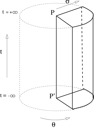
Figure 5: The region $Z_{0}$ in $\widetilde{SL}_{2}({\bf R})$. It is the universal covering space of $Y_{(-\frac{\gamma^{2}l}{16G},-\frac{\tilde{\gamma}^{2}l}{16G})}$.

The ranges are $-\infty<t<+\infty,\ 0\leq\theta<\pi(\gamma+\tilde{\gamma})$ and $0<\sigma<+\infty$. The projection $\pi$ causes a conical singularity at $\sigma=0$ (Fig.6).

Figure 6: $Y_{(-\frac{\gamma^{2}l}{16G},-\frac{\tilde{\gamma}^{2}l}{16G})}$. The dotted wavy line denotes a conical singularity which will be added to $Y_{(-\frac{\gamma^{2}l}{16G},-\frac{\tilde{\gamma}^{2}l}{16G})}$ after the completion at $\sigma=0$.

Mathematically speaking, $\pi:Z_{0}\rightarrow Y_{(-\frac{\gamma^{2}l}{16G},-\frac{\tilde{\gamma}^{2}l}{16G})}$ is regular but, once we make the completion of $Z_{0}$ at $\sigma=0$ by adding the line $PP^{{}^{\prime}}$ and extend $\pi$ to this line, it becomes singular. This singular mapping causes the conical singularity. In particular, when $\gamma=\tilde{\gamma}$, the appearance of the conical singularity is due to a particle with mass $\frac{1-\gamma}{4G}$ sitting at $\sigma=0$ [23].

4.3.2 How can we understand $3d$ black holes in two dimensions ?

Having obtained the correspondence between the states of the three-dimensional quantum gravity and the two-dimensional conformal field theory, one may ask how the three-dimensional black holes can be understood in two dimensions where the conformal field lives.

To investigate this question, it is useful to discuss first the case of the conical sigularities. The state $|k_{\gamma}\rangle_{in}\otimes|\tilde{k}_{\tilde{\gamma}}\rangle_{in}$ of the conical singularity can be obtained by an operation of the corresponding vertex operator on the $sl_{2}(\bf{C})$-invariant vacuum,

$$|\gamma,\tilde{\gamma}\rangle_{in}=\lim_{z,\bar{z}\rightarrow 0}e^{ik_{\gamma}X(z)}e^{i\tilde{k}_{\tilde{\gamma}}X(\bar{z})}|vac\rangle_{in}.$$ (4.32)

Making the holomorphic and anti-holomorphic pieces together, we will rewrite the above operator into the form,

$$e^{ik_{\gamma}X(z)}e^{i\tilde{k}_{\tilde{\gamma}}X(\bar{z})}=\displaystyle{e^{\sqrt{\frac{l}{8G}}(1-\frac{\gamma+\tilde{\gamma}}{2})X(z,\bar{z})-\sqrt{\frac{l}{8G}}\frac{\gamma-\tilde{\gamma}}{2}\widetilde{X}(z,\bar{z})}},$$ (4.33)

where $X(z,\bar{z})=X(z)+X(\bar{z})$ and $\widetilde{X}(z,\bar{z})\equiv X(z)-X(\bar{z})$ . If one takes the path-integral formulation of $2d$ CFT, the norm of this state, which should be normalized to unity, can be written in the following manner :

$${}_{out}\langle\gamma,\tilde{\gamma}|\gamma,\tilde{\gamma}\rangle_{in}$$

$$=\int DXe^{-S}\cdot e^{\sqrt{\frac{l}{8G}}(1+\frac{\gamma+\tilde{\gamma}}{2})X(\infty)+\sqrt{\frac{l}{8G}}\frac{\gamma-\tilde{\gamma}}{2}\widetilde{X}(\infty)}\cdot e^{\sqrt{\frac{l}{8G}}(1-\frac{\gamma+\tilde{\gamma}}{2})X(0)-\sqrt{\frac{l}{8G}}\frac{\gamma-\tilde{\gamma}}{2}\widetilde{X}(0)}$$ (4.34)

where $S$ is the action (4.10) with $\alpha_{0}=\sqrt{\frac{l}{8G}}$. The vertex operators inserted at $0$ and $\infty$ respectively create the states of the conical singularity from the $sl_{2}({\bf C})$ invariant in- and out- vacua. Choosing the background metric so that its curvature concentrates at $\infty$, we rewrite the expression (4.34) in the following form :

$${}_{out}\langle\gamma,\tilde{\gamma}|\gamma,\tilde{\gamma}\rangle_{in}$$

$$=\int DXe^{-\frac{1}{4\pi i}\int\bar{\partial}X\wedge\partial X}\cdot e^{-\sqrt{\frac{l}{8G}}(1-\frac{\gamma+\tilde{\gamma}}{2})X(\infty)+\sqrt{\frac{l}{8G}}\frac{\gamma-\tilde{\gamma}}{2}\widetilde{X}(\infty)}\cdot e^{\sqrt{\frac{l}{8G}}(1-\frac{\gamma+\tilde{\gamma}}{2})X(0)-\sqrt{\frac{l}{8G}}\frac{\gamma-\tilde{\gamma}}{2}\widetilde{X}(0)}.$$

(4.35)

The Liouville field $X$ treats the conical singularity as an insertion of the corresponding vertex operator. This vertex operator has the following origin in three-dimensions. To explain this, we first remark that the ${\bf P}^{1}$ where the Liouville field theory lives can be regarded as that obtained by a compactification of the boundary cylinder at infinity. This compactification also makes the solid cylinder to a three-dimensional ball. In such a compactification to a three-ball, the conical sigularity located at the center must intersect with the ${\bf P}^{1}$ precisely at the two points, $0$ and $\infty$. See Fig.7.

Figure 7: The conical singularity seen by the boundary Liouville field $X$

Now, back to the path-integral expression given in (4.35), we can say that these intersections of the conical singularity with the boundary sphere are realized as the vertex operators in the boundary Liouville field theory. In particular, the gravitational state of a particle with mass $\frac{1-\gamma}{4G}$ sitting at the center of $AdS_{3}$ can be treated by an insertion of the corresponding vertex operator.

Nextly let us discuss about the case of the black holes. Basically we follow the same argument as above. The black hole state (4.27) can be obtained by an operation of the corresponding vertex operator on the $sl_{2}(\bf{C})$-invariant vacuum,

$$|J,M\rangle_{in}=\lim_{z,\bar{z}\rightarrow 0}\displaystyle{e^{(\sqrt{\frac{l}{8G}}+i\frac{r_{+}}{\sqrt{8Gl}})X(z,\bar{z})+i\frac{r_{-}}{\sqrt{8Gl}}\widetilde{X}(z,\bar{z})}}|vac\rangle_{in}.$$ (4.36)

If one takes the path-integral formulation, the norm of the black hole state can be written in the following manner :

$${}_{out}\langle J,M|J,M\rangle_{in}$$

$$~{}~{}~{}~{}~{}=\int DXe^{-\frac{1}{4\pi i}\int\bar{\partial}X\wedge\partial X}\cdot e^{-(\sqrt{\frac{l}{8G}}+i\frac{r_{+}}{\sqrt{8Gl}})X(\infty)-i\frac{r_{-}}{\sqrt{8Gl}}\widetilde{X}(\infty)}\cdot e^{(\sqrt{\frac{l}{8G}}+i\frac{r_{+}}{\sqrt{8Gl}})X(0)+i\frac{r_{-}}{\sqrt{8Gl}}\widetilde{X}(0)}.$$

(4.37)

This path-integral representation also provides some idea about our interpretation of the black holes in the two dimensions.

We first remark that the outer horizon of the black hole can not be recognized as a two-dimensional object under the Virasoro deformation. See Fig.3 for the non-extremal case. It is treated as a one-dimensional object for the massive black hole, and as a point for the massless black hole. The Virasoro deformation is originally introduced as a deformation of the non-compact simply-connected region $Z_{0}$. This region of $SL_{2}({\bf R})$ is the covering space of the exterior of the outer horizon of the black hole. Under the Virasoro deformation what one can recognize as the outer horizon is the counterpart of the outer horizon on $SL_{2}({\bf R})$. It is obtained by the completion of $Z_{0}$ at $\sigma=0$. We can easily see that these completions for the cases of the massive extremal and massless black holes are respectively given by adding one-dimensional and zero-dimensional objects. Being zero-dimensional in the massless case may be understood as a degeneration from the massive case.

We hope to explain the geometrical origin of the insertion of the vertex operator in (4.37). Let us examine first the compactification of the boundary cylinder of the black hole $X^{+}_{(J,M)}$ to the ${\bf P}_{1}$. $t=\pm\infty$ circles of the boundary cylinder are mapped to the two points $0$ and $\infty$ of the ${\bf P}_{1}$. This compactification of the boundary also provide a compactification of the bulk geometry. Now we will ask what it gives rise to. We can assume reasonably that $t=\pm\infty$ slices of $X_{(J,M)}^{+}$ are compactified to $0$ and $\infty$ of the ${\bf P}_{1}$. If one accepts this assumption, the outer horizon must be compactified to $0$ and $\infty$ of ${\bf P}_{1}$. This is because the $t=\pm\infty$ slices of $X_{(J,M)}^{+}$ include the outer horizon after the completion. See Fig.3. This shows that the intersections of the black hole with the boundary sphere are realized by the vertex operators as described in (4.37). See Fig.8.

Figure 8: The black hole seen by the boundary Liouville field $X$

5 Towards Conformal Field Theory On The Horizon

To provide a microscopic description of black holes in quantum gravity or string theory is a very impressive and enlightening issue. For the three-dimensional black holes such a microscopic description has been proposed by Carlip [8] and Strominger [9, 10]. It states that microscopic states of the black holes are the states of a conformal field theory on the horizon. Although at present we do not know exactly what conformal fields do live on the horizon, their proposal makes it possible to give statistical mechanical explanations of the thermodynamical properties of the black hole.

Receiving their proposal, many questions will arise. First of all, can one identify the boundary Liouville field theory with a conformal field theory on the horizon ? Our answer is NO. As explained at the end of the last section, the Virasoro deformation of the exterior of the outer horizon can not recognize the horizon as a two-dimensional object. It can recognize the horizon only as a one-dimensional object. This means that the Virasoro algebra obtained from the deformation cannot be the Virasoro algebra on the horizon. On the other hand, this deformation provides the asymptotic Virasoro algebra, which generators are gravitons in bulk and are identified with the excitations of the boundary Liouville field. This field theory has the continuous spectrums. Therefore these two conformal field theories are by no means equivalent to each other.

If one accepts this answer, one might be led to another question : What conformal field theory is living on the horizon ? To this question we can not answer definitely. Here we would like to propose two possible descriptions of this conformal field theory. The first one is based on a simple hypothesis : The Virasoro algebra of the horizon conformal field theory should generate the Virasoro deformation of the horizon. To work this hypothesis, we need, first of all, to treat the outer horizon as a two-dimensional object. If one takes the Chern-Simons gravity viewpoint, it is doubtful whether one can handle the outer horizon as a two-dimensional object. To be successful, presumably one needs the string theory viewpoint. Namely, if the two-dimensional horizon is identified with a macroscopic string in $SL_{2}({\bf R})$, the horizon conformal field theory would be string theory on this background. It describes quantum fluctuations of the macroscopic string and will lead the microscopic description of the black holes. But it is not clear, at least for us, to what extent this string theory is analyzable.

The second possible description of the horizon conformal field theory is based on the hypothesis : The Virasoro deformation of the region between the inner and outer horizons should lead the Virasoro algebra on the horizon conformal field theory. This hypothesis can be regarded as an analogue which we used in the construction of the boundary Liouville field theory. In particular it may allow us to follow the similar step as we took for the study of the exterior of the outer horizon.

To be explicit, let us consider the region between the inner and outer horizons of the non-extremal BTZ black hole $X_{(J,M)}$. We will call it $X_{(J,M)}^{-}$ . A covering space of $X_{(J,M)}^{-}$ is given by a non-compact simply-connected region of $SL_{2}({\bf R})$ consisting of the group elements

$$e^{-\varphi J^{2}}e^{\sigma J^{0}}e^{\psi J^{2}},$$ (5.1)

where the ranges of $\varphi,\psi$ and $\sigma$ are taken $-\infty<\varphi,\psi<+\infty$ and $0<\sigma<\pi$. Let us call this region $Z_{1}$. The projection can be described by

$$\frac{r_{+}+r_{-}}{l}\left(\frac{t}{l}+\phi\right)=\varphi,~{}~{}~{}\frac{r_{+}-r_{-}}{l}\left(\frac{t}{l}-\phi\right)=\psi,~{}~{}~{}\frac{2r^{2}-r_{+}^{2}-r_{-}^{2}}{r_{+}^{2}-r_{-}^{2}}=\cos\sigma,$$ (5.2)

together with the identification $\phi\sim\phi+2\pi$. The induced metric of $Z_{1}$ has the form

$${ds}^{2}_{1}=\frac{l^{2}}{4}\left\{(d\varphi)^{2}+(d\psi)^{2}-2\cos\sigma~{}d\varphi d\psi-(d\sigma)^{2}\right\},$$ (5.3)

and is isometric to $ds_{X_{(J,M)}^{-}}^{2}$. Therefore $Z_{1}$ is indeed the covering space. $X_{(J,M)}^{-}$ is identified with the quotient of $Z_{1}$,

$$X^{-}_{(J,M)}=Z_{1}/\sim,$$ (5.4)

where the equivalence relation is $(\varphi,\psi,\sigma)\sim(\varphi+2\pi\frac{r_{+}+r_{-}}{l},\psi-2\pi\frac{r_{+}-r_{-}}{l},\sigma)$. As is done in the study of $Z_{0}$, it is convenient to rewrite the group element (5.1) in the form

$$e^{-\sqrt{\frac{b_{0}}{c/24}}wJ^{2}}e^{(\rho-\frac{1}{2}\ln\frac{b_{0}\tilde{b}_{0}}{(c/6)^{2}})J^{0}}e^{\sqrt{\frac{\tilde{b}_{0}}{c/24}}\tilde{w}J^{2}}~{}~{}~{}(\equiv h_{1}(w,\tilde{w},\rho)).$$ (5.5)

Description of $Z_{1}$ in terms of the Chern-Simons gravity is given by the flat connection $A_{1}=(A_{1}^{(+)},A_{1}^{(-)})$ which is determined by the prescription (2.19) using a decomposition of $h_{1}$ into the following $SL_{2}({\bf R})_{\pm}$-valued functions $h^{(\pm)}_{1}$ :

$${h}_{1}^{(+)}=e^{-\frac{1}{2}(\rho-\ln\frac{b_{0}}{c/6})J^{0}}e^{\sqrt{\frac{b_{0}}{c/24}}wJ^{2}},~{}~{}~{}~{}{h}_{1}^{(-)}=e^{\frac{1}{2}(\rho-\ln\frac{\tilde{b}_{0}}{c/6})J^{0}}e^{\sqrt{\frac{\tilde{b}_{0}}{c/24}}\tilde{w}J^{2}}.$$ (5.6)

A slight comparison between $h_{1}^{(\pm)}$ and $h^{(\pm)}$ given in (2.28) shows that the flat connection $A_{1}$ is gauge-equivalent to $A_{0}$ (2.33), the flat connection which describes $Z_{0}$, the covering space of the exterior of the horizon :

$$A_{1}=A_{0}^{g},$$ (5.7)

where the gauge transformation $g=(g^{(+)},g^{(-)})$ is given by $g^{(+)}=e^{-\frac{1}{2}(\rho-\ln\frac{b_{0}}{c/6})J^{0}}e^{\frac{1}{2}(\rho-\ln\frac{b_{0}}{c/6})J^{1}}$ and $g^{(-)}=e^{\frac{1}{2}(\rho-\ln\frac{\tilde{b}_{0}}{c/6})J^{0}}e^{-\frac{1}{2}(\rho-\ln\frac{\tilde{b}_{0}}{c/6})J^{1}}$. This gauge equivalence should be understood as a formal one because the allowed ranges of the coordinates are different from each other. (For $A_{0}$ (2.33) the range of $\rho$ is $\frac{1}{2}\ln\frac{b_{0}\tilde{b}_{0}}{(c/6)^{2}}<\rho<+\infty$ while for $A_{1}$, $\frac{1}{2}\ln\frac{b_{0}\tilde{b}_{0}}{(c/6)^{2}}<\rho<\pi+\frac{1}{2}\ln\frac{b_{0}\tilde{b}_{0}}{(c/6)^{2}}$ .) Nevertheless, if one takes the existence of such a gauge transformation seriously, one may arrive at an idea that a deformation of $Z_{1}$ could be constructed in such a manner that it is related with the Virasoro deformation of $Z_{0}$ by an appropriate gauge transformation. Thus obtained deformation will define the Virasoro deformation of $Z_{1}$ and thereby that of $X_{(J,M)}^{-}$, the region between the inner and outer horizons of the black hole. The corresponding conformal field theory will be regarded as the horizon conformal field theory.

The second description of the horizon conformal field theory may provide another interpretation of the surprising conjecture made by Maldacena [1], which may be understood in our situation as a correspondence between the boundary and horizon conformal field theories under a suitable renormalization group flow. The second description, if it is correct, implies a possibility of a realization of this correspondence in terms of gauge transformation.

We thank S. Mano for useful discussions.

Note Added

After this work was completed we received a preprint [24] in which the content of 3.3 is also discussed.

References

- [1] J. Maldacena, “The Large Limit Of Superconformal Field Theories And Supergravity”, Adv. Theor. Math. Phys. 2 (1998) 231, hep-th/9711200
- [2] S.S. Gubser, I.R. Klebanov and A.M. Polyakov, “Gauge Theory Correlators From Non-critical String Theory”, Phys. Letts. B428 (1998) 105.
- [3] E. Witten, “Anti de Sitter Space And Holography”, Adv. Theor. Math. Phys. 2 (1998) 253.
- [4] E. Witten, “2+1 DIMENSIONAL GRAVITY AS AN EXACTLY SOLUBLE SYSTEM”, Nucl. Phys. B311 (1988/89) 46.
- [5] J.D. Brown and M. Henneaux, “Central Charges in the Canonical Realization of Asymptotic Symmetries: An Example from Three Dimensional Gravity”, Commn. Math. Phys. 104 (1986) 207.
- [6] M. Banados, “Three dimensional quantum geometry and black holes”, hep-th/9901148.
- [7] E.J. Martinec, “Conformal Field Theory, Geometry and Entropy”, hep-th/9809021.
- [8] S. Carlip, “Statistical mechanics of the (2+1)-dimensional black hole”, Phys. Rev. D51 (1995) 632.
- [9] A. Strominger, “Black Hole Entropy from Near-Horizon Microstates”, JHEP 9802 (1998) 009.
- [10] J. Maldacena and A. Strominger, “ Black Holes and a Stringy Exclusion Principle”, JHEP 9812 (1998) 005.
- [11] M. Banados, C. Teitelboim and J. Zanelli, “Black Hole in Three-Dimensional Spacetime”, Phys. Rev. Lett. 69 (1992) 1849.
- [12] M. Banados, M. Henneaux, C. Teitelboim and J. Zanelli, “Black Hole in Three-Dimensional Spacetime”, Phys. Rev. D48 (1993) 1506.
- [13] A. Achúcarro and P.K. Townsend, “A Chern-Simons Action for Three-dimensional Anti-de Sitter Supergravity theories”, Phys. Lett. 180B (1986) 89.
-
[14]
O. Coussaert, M. Henneaux and P.Van. Driel,
“The asymptotic dynamics of three-dimensional Einstein gravity
with a negative cosmological constant”,
Class. Quant. Grav. 12 (1995) 2961,
M. Banados and M. Ortiz, “The central charge in three-dimensional anti-de Sitter space”, hep-th/9806089. - [15] A.M. Polyakov, “GAUGE TRANSFORMATIONS AND DIFFEOMORPHISMS”, Int. J. Mod. Phys. A5 (1990) 833.
- [16] For an example, N.M.J. Woodhouse, “Geometric Quantization”, Second edition, Oxford Mathematical Monograph, Oxford 1991.
- [17] E. Witten, “COADJOINT ORBITS OF THE VIRASORO GROUP”, Commun. Math. Phys. 114 (1988) 1.
- [18] G. Segal, “Unitary Representations of Some Infinite Dimensional Groups”, Commun. Math. Phys. 80 (1981) 307.
- [19] M.J. Bowick and S.G. Rajeev, “THE HOLOMORPHIC GEOMETRY OF CLOSED BOSONIC STRING THEORY AND ”, Nucl. Phys. B293 (1987) 348.
- [20] A. Fujii, R. Kemmoku and S. Mizoguchi, “ simple supergravity on and superconformal field theory”, hep-th/9811147.
- [21] S. Carlip and C. Teitelboim, “Aspects of black hole quantum mechanics and thermodynamics in 2+1 dimensions”, Phys. Rev. D51 (1995) 622.
- [22] J.E. Nelson, T. Regge and F. Zertuche, “Homotopy Groups And (2+1)-Dimensional Quantum de Sitter Gravity”, Nucl. Phys. B339 (1990) 516.
- [23] S. Deser and R. Jackiw, “Three-Dimensional Cosmological Gravity: Dynamics of Constant Curvature”, Ann. Phys. (N.Y.) 153 (1984) 405.
- [24] J. Navarro-Salas and P. Navarro, “Virasoro Orbits, AdS(3) Quantum Gravity And Entropy”, hep-th/9903248.