hep-th/9903215

UTHEP-400

March, 1999

N=2 Superconformal Field Theory with ADE Global Symmetry on a D3-brane Probe

Masayuki Noguchi, Seiji Terashima and Sung-Kil Yang
Institute of Physics, University of Tsukuba
Ibaraki 305-8571, Japan
Abstract

We study mass deformations of $N=2$ superconformal field theories with $ADE$ global symmetries on a D3-brane. The $N=2$ Seiberg-Witten curves with $ADE$ symmetries are determined by the Type IIB 7-brane backgrounds which are probed by a D3-brane. The Seiberg-Witten differentials $\lambda$ for these $ADE$ theories are constructed. We show that the poles of $\lambda$ with residues are located on the global sections of the bundle in an elliptic fibration. It is then clearly seen how the residues transform in an irreducible representation of the $ADE$ groups. The explicit form of $\lambda$ depends on the choice of a representation of the residues. Nevertheless the physics results are identical irrespective of the representation of $\lambda$. This is considered as the global symmetry version of the universality found in $N=2$ Yang-Mills theory with local $ADE$ gauge symmetries.

1 Introduction

Probing the 7-brane background of Type IIB compactification on ${\bf P}^{1}$ by a D3-brane provides a powerful machinery to analyze the non-perturbative behavior of four-dimensional $N=2$ supersymmetric gauge theories [1, 2]. In this setup, the space-time gauge symmetry is transmuted into the global symmetry in the world volume $N=2$ supersymmetric gauge theory on a D3-brane. Then it is found in [3] that there exist non-trivial $N=2$ superconformal fixed points with exceptional global symmetries. In [4, 5], on the other hand, $N=2$ fixed points with $E_{n}$ global symmetries are considered as a natural extension of foregoing works [6, 7, 8, 9].

Although the $N=2$ theory with exceptional symmetry does not admit the Lagrangian description, recent advances in string duality have made it possible to study the strong-coupling regime of $N=2$ theory by the stringy technique. For instance, it requires a considerable amount of effort in general to analyze the properties of the BPS spectrum of $N=2$ theory. The junction picture of BPS states, however, gives the simple constraint on the BPS spectrum [10, 11]. With the use of this constraint, some characteristic features of the BPS states in $N=2$ theory with $E_{n}$ symmetries are revealed [11].

In this paper we study mass deformations of $N=2$ theories with $ADE$ global symmetries in detail. The present work is partly motivated in our attempt to get a clearer understanding of the results obtained by Minahan and Nemeschansky [4, 5] in formulating the elliptic curves and the Seiberg-Witten (SW) differentials for $E_{n}$ theories. It was found in [5] that, for a given elliptic curve, the SW differential $\lambda$ is not uniquely determined, but depends on the representations (fundamental or adjoint) of the global symmetry group. It is then argued that $\lambda$ in different representations lead to different physics.

In our approach we proceed along the line of the D3-brane probe picture and discuss systematically the curves and the differentials for the $ADE$ theories. In particular we clarify a great deal the properties of the pole terms of the SW differential. Even for the case of $N=2$ $SU(2)$ QCD with $N_{f}\leq 3$, which is thought to be well understood, we gain a new insight. Consequently we are able to show that the representations of the ADE groups from which the SW differential is built are irrelevant to the physics results. In this regard, our conclusion is opposed to what is argued in [5].

The paper is organized as follows. In section 2, we see that the elliptic curves for $N=2$ $ADE$ theories on a D3-brane are naturally identified by examining the local geometry of singularities in the compactification of Type IIB theory on ${\bf P}^{1}$ with the 24 background 7-branes. In section 3 the BPS mass formula for $N=2$ $ADE$ theories is discussed in the light of the string junction lattice. In section 4 the residues of the poles of the SW differentials for our $ADE$ theories are shown to transform in an irreducible representation of the global symmetry groups. This affords a firm foundation of somewhat empirical construction of the SW differentials in [6, 4, 5]. In section 5 the SW differentials in the fundamental as well as the adjoint representations are obtained in the $A_{1},\;A_{2},\;D_{4},\;E_{6},\;E_{7}$ and $E_{8}$ theories. In section 6 we analyze in detail how the SW differential behaves under the renormalization group flow from the $E_{6}$ theory to the $D_{4}$ theory. In section 7 it is proved that the SW periods are independent of the representations of the global symmetry which are chosen to construct the SW differential. The result in section 7 is confirmed in section 8 by further studying $N=2$ $SU(2)$ QCD with $N_{f}\leq 3$. Finally we conclude in section 9.

2 D3-brane probe and elliptic curves

When Type IIB theory is compactified on ${\bf P}^{1}$ with the 24 background 7-branes, the string coupling constant $\tau=\chi+ie^{-\phi}$, where $\chi$ is a R-R scalar field and $\phi$ a dilaton, is determined as the modular parameter of an elliptic curve [12]

$$y^{2}=x^{3}+f(z)x+g(z).$$ (2.1)

Here $z$ is a complex coordinate on ${\bf P}^{1}$, $f$ and $g$ are polynomials in $z$ of degree 8 and 12, respectively. The 24 zeroes of the discriminant $\Delta=4f^{3}+27g^{2}$ are the transverse positions of the 24 7-branes. The modular parameter $\tau$ is obtained from $j(\tau)=4(24f)^{3}/\Delta$. The cubic (2.1) describes a $K3$ surface as an elliptic fibration over the base ${\bf P}^{1}$. When the positions of some 7-branes coincide the elliptic fibration develops singularities which are well-known to follow the Kodaira classification [13]. The singularity types then have a correspondence with the $ADE$ singularities, according to which the $ADE$ types of gauge symmetry in Type IIB theory are identified [1, 14].

The connection between the $ADE$ gauge symmetry and the background 7-brane configurations has been established by analyzing the monodromy properties [15, 16]. In Type IIB theory there exist 7-branes which are mutually nonlocal. To distinguish them we shall refer to a 7-brane on which Type IIB $(p,q)$ strings can end as a $[p,q]$ 7-brane. For the purpose of describing the $ADE$ symmetry it is sufficient to take into account $[1,0]$, $[1,-1]$ and $[1,1]$ 7-branes which will be henceforth denoted as ${\bf A}$-, ${\bf B}$- and ${\bf C}$-branes, respectively. Let ${\bf A}^{n}{\bf B}^{m}{\bf C}^{\ell}$ represent a set of $n$ ${\bf A}$-, $m$ ${\bf B}$- and $\ell$ ${\bf C}$-branes. The $E_{8}$ gauge symmetry, for instance, is realized at $\tau=e^{2\pi i/3}$ when a set of 7-branes ${\bf A}^{7}{\bf B}{\bf C}^{2}$ coalesces. Gauge symmetries and the corresponding 7-brane configurations relevant to our following discussions are summarized in Table 1. We note that $E_{5}=D_{5}$ and the brane configuration ${\bf A}^{4}{\bf B}{\bf C}^{2}$ is shown to be equivalent to ${\bf A}^{5}{\bf B}{\bf C}$ [17].

gauge	Kodaira	background	coupling
symmetry	type	7-branes	constant $\tau$
$E_{8}$	${\rm II}^{*}$	${\bf A}^{7}{\bf B}{\bf C}^{2}$	$e^{2\pi i/3}$
$E_{7}$	${\rm III}^{*}$	${\bf A}^{6}{\bf B}{\bf C}^{2}$	$i$
$E_{6}$	${\rm IV}^{*}$	${\bf A}^{5}{\bf B}{\bf C}^{2}$	$e^{2\pi i/3}$
$E_{5}$	${\rm I}^{*}_{1}$	${\bf A}^{4}{\bf B}{\bf C}^{2}$	$\infty$
$D_{4}$	${\rm I}^{*}_{0}$	${\bf A}^{4}{\bf B}{\bf C}$	arbitrary
$A_{2}$	${\rm IV}$	${\bf A}^{3}{\bf C}$	$e^{2\pi i/3}$
$A_{1}$	${\rm III}$	${\bf A}^{2}{\bf C}$	$i$
$\{0\}$	${\rm II}$	${\bf A}{\bf C}$	$e^{2\pi i/3}$

Table 1: Symmetry and background 7-branes

We now introduce a D3-brane which is parallel to the background 7-branes. This D3-brane can probe the local geometry near the singularities which are responsible for the gauge symmetry enhancement. On the D3-brane the low-energy effective theory becomes four-dimensional $N=2$ supersymmetric gauge theory. Suppose that the D3-brane probe is located near coalescing 7-branes, then $N=2$ theory on the D3-brane is a fixed point theory since there are no relevant mass parameters turned on. The gauge symmetry in the bulk turns out to be the enhanced global symmetry of a fixed-point $N=2$ supersymmetric theory on the brane [2].

From this point of view, let us look at Table 1. First of all, the $D_{4}$ theory on the brane in the vicinity of the 7-branes ${\bf A}^{4}{\bf B}{\bf C}$ arises in $N=2$ $SU(2)$ theory with $N_{f}=4$ fundamental quarks [6]. Here ${\bf B}$- and ${\bf C}$-branes stand for monopole and dyon singularities, and ${\bf A}$-branes stand for the squark singularities in the Coulomb branch. The $N=2$ $SU(2)$ theory with $N_{f}=4$ is finite and the marginal gauge coupling constant can take any values. Similarly, the $A_{2}$, $A_{1}$ and $\{0\}$ theories also arise in the Coulomb branch of $N=2$ $SU(2)$ theory with $N_{f}=3$, 2 and 1, respectively. These are non-trivial superconformal theories obtained by adjusting quark masses at particular values [8]. On the other hand, the $D_{5}$ theory describes the IR free behavior of $N=2$ $SU(2)$ theory with $N_{f}=5$. The most interesting are the theories with $E_{n}$ $(n=6,7,8)$ global symmetries. They are non-trivial $N=2$ superconformal field theories, but do not admit the Lagrangian description. In view of the D3-brane probe approach, it is natural to place these non-trivial fixed points with exceptional symmetry in the sequence of renormalization group flows

$$E_{8}\;{\mathop{\hbox to36.98866pt{\rightarrowfill}}\limits_{\bf A}}\;E_{7}\;{\mathop{\hbox to36.98866pt{\rightarrowfill}}\limits_{\bf A}}\;E_{6}\;{\mathop{\hbox to36.98866pt{\rightarrowfill}}\limits_{{\bf A},\,{\bf C}}}\;D_{4}\;{\mathop{\hbox to36.98866pt{\rightarrowfill}}\limits_{{\bf A},\,{\bf B}}}\;A_{2}\;{\mathop{\hbox to36.98866pt{\rightarrowfill}}\limits_{\bf A}}\;A_{1}\;{\mathop{\hbox to36.98866pt{\rightarrowfill}}\limits_{\bf A}}\;\{0\},$$ (2.2)

where 7-branes indicated under the arrows are sent to infinity to generate the flows. In (2.2) only the $D_{4}$ theory is described as a local Lagrangian field theory, while the others are considered to be non-local. Note that the flows $E_{6}\rightarrow D_{4}$ and $D_{4}\rightarrow A_{2}$ are realized by moving away mutually non-local 7-branes simultaneously.

Starting with the $D_{4}$ theory one can also consider more familiar flows

$$D_{4}\;{\mathop{\hbox to36.98866pt{\rightarrowfill}}\limits_{\bf A}}\;D_{3}\;{\mathop{\hbox to36.98866pt{\rightarrowfill}}\limits_{\bf A}}\;D_{2}\;{\mathop{\hbox to36.98866pt{\rightarrowfill}}\limits_{\bf A}}\;D_{1}\;{\mathop{\hbox to36.98866pt{\rightarrowfill}}\limits_{\bf A}}\;D_{0}\,,$$ (2.3)

where the 7-brane background for the $D_{n}$ symmetry is given by ${\bf A}^{n}{\bf B}{\bf C}$. Note that, for $n\leq 3$, the configuration ${\bf A}^{n}{\bf B}{\bf C}$ does not fall into the Kodaira classification since it is non-collapsible [17]. On a D3-brane probing ${\bf A}^{n}{\bf B}{\bf C}$ with $n\leq 3$, ordinary $N=2$ $SU(2)$ QCD with $N_{f}=n$ fundamental quarks is realized.

As mentioned previously, enhanced global symmetries at the fixed points in (2.2) are recognized in geometric terms as the $ADE$ singularities. Thus relevant perturbations taking the system away from criticality are described in terms of versal deformations of the $ADE$ singularities. The coupling constant $\tau$ of deformed $N=2$ theories is then determined by elliptic curves in the form of (2.1) where the explicit forms of polynomials $f$ and $g$ are now specified by the $ADE$ singularity types. We have

$$E_{8}: f=w_{2}z^{3}+w_{8}z^{2}+w_{14}z+w_{20}, g=z^{5}+w_{12}z^{3}+w_{18}z^{2}+w_{24}z+w_{30},$$ (2.4)

$$E_{7}: f=z^{3}+w_{8}z+w_{12}, g=w_{2}z^{4}+w_{6}z^{3}+w_{10}z^{2}+w_{14}z+w_{18},$$ (2.5)

$$E_{6}: f=w_{2}z^{2}+w_{5}z+w_{8}, g=z^{4}+w_{6}z^{2}+w_{9}z+w_{12},$$ (2.6)

$$D_{4}: f=z^{2}+\widetilde{w}_{4}, g=w_{2}z^{2}+w_{4}z+w_{6},$$ (2.7)

$$A_{2}: f=w_{2}, g=z^{2}+w_{3},$$ (2.8)

$$A_{1}: f=z, g=w_{2},$$ (2.9)

where the $w_{q}$ are deformation parameters. Here $z$ is understood as the gauge invariant expectation value which parametrizes the vacuum moduli of $N=2$ theory. In the brane picture $z$ is a coordinate of the position of the D3-brane probe on ${\bf P}^{1}$. In the cubic (2.1) with (2.4)-(2.9) we take $y^{2}$ to be of degree $h$ with $h$ being the Coxeter number of $G=ADE$ (see Table 2). Then $x,y,z$ have the degree $q_{x},q_{y},q_{z}$ as given in Table 2 and $w_{q_{i}}$ has the degree $q_{i}=e_{i}+1$ where $e_{i}$ is the $i$-th exponent of $G$. Note here that $q_{x}+q_{z}=q_{y}+1$ and $2q_{y}=h$. The value of $q_{z}$ gives the scaling dimension of the expectation value $z$ [8, 4].

	$E_{8}$	$E_{7}$	$E_{6}$	$D_{4}$	$A_{2}$	$A_{1}$
$h$	30	18	12	6	3	2
$q_{y}$	15	9	6	3	3/2	1
$q_{x}$	10	6	4	2	1	2/3
$q_{z}$	6	4	3	2	3/2	4/3

Table 2: Degree of variables

Notice that only in the $D_{4}$ theory the coupling constant $\tau$ is marginal, and hence the curve may incorporate the $\tau$-dependence. This is allowed since $x$ and $z$ have the same degree $q_{x}=q_{z}=2$ which holds only for the $D_{4}$ case. In fact the Seiberg-Witten (SW) curve for the $D_{4}$ theory obtained originally in [6] depends on both $\tau$ and four bare quark masses $m_{1},m_{2},m_{3},m_{4}$. It is not difficult to work out how the SW curve in [6] is related to our $D_{4}$ curve (2.7). Let us write down the SW curve presented in (17.58), section 17 of [6]

$$Y^{2}=X(X-\alpha Z)(X-\beta Z)+aX^{2}+bX+cZ+d,$$ (2.10)

where we have used $Z$ instead of $u$ to denote the adjoint Higgs expectation value and

$$a=(\alpha-\beta)^{2}u_{2}/4,\hskip 28.45274ptb=-(\alpha-\beta)^{2}\alpha\beta u_{4}/4+i\alpha\beta(\alpha^{2}-\beta^{2})\widetilde{u}_{4}/4,$$

$$c=-i(\alpha-\beta)\alpha^{2}\beta^{2}\widetilde{u}_{4}/2,\hskip 28.45274ptd=(\alpha-\beta)^{2}\alpha^{2}\beta^{2}u_{6}/4,$$

$$\alpha=-\vartheta_{3}^{4}(\tau),\hskip 28.45274pt\beta=-\vartheta_{4}^{4}(\tau),$$

$$\vartheta_{3}(\tau)=\sum_{n\in{\bf Z}}q^{n^{2}/2},\hskip 28.45274pt\vartheta_{4}(\tau)=\sum_{n\in{\bf Z}}(-1)^{n}q^{n^{2}/2},\hskip 28.45274ptq=e^{2\pi i\tau}.$$ (2.11)

Here the $D_{4}$ invariants made of quark masses are defined by

$$u_{2}=-\sum_{a}m_{a}^{2},\hskip 28.45274ptu_{4}=\sum_{a<b}m_{a}^{2}m_{b}^{2},$$

$$u_{6}=-\sum_{a<b<c}m_{a}^{2}m_{b}^{2}m_{c}^{2},\hskip 28.45274pt\widetilde{u}_{4}=-2im_{1}m_{2}m_{3}m_{4}.$$ (2.12)

Making a change of variables

$$X=-\alpha\beta x,\hskip 28.45274ptY=\alpha\beta(\alpha-\beta)y/2,\hskip 28.45274ptZ=i(\alpha-\beta)z/2-(\alpha+\beta)x/2,$$ (2.13)

we see that (2.10) becomes

$$y^{2}=xz^{2}+x^{3}+u_{2}x^{2}+u_{4}x+\widetilde{u}_{4}z+u_{6}$$ (2.14)

which is nothing but the standard form of deformations of the $D_{4}$ singularity. We next replace $x$ by $x-u_{2}/3$ and shuffle the $D_{4}$ invariants as

$$u_{2}=-3w_{2},\hskip 28.45274ptu_{4}=\widetilde{w}_{4}+3w_{2}^{2},$$

$$u_{6}=w_{6}-w_{2}\widetilde{w}_{4}-w_{2}^{3},\hskip 28.45274pt\widetilde{u}_{4}=w_{4}.$$ (2.15)

Then we obtain the $D_{4}$ curve with (2.7).

3 BPS mass formula

Having obtained the SW curve for $N=2$ theory on a D3-brane probe, we next discuss the BPS mass formula. In the brane probe approach, BPS states on the D3-brane world volume are geometrically realized as Type IIB strings, or more generally string junctions obeying the BPS condition. According to [18], junctions are specified by asymptotic charges $(p,q)$ and a weight vector of $G=ADE$. Denoting a junction as ${\bf J}$ we have [18]

$${\bf J}=p\mbox{\boldmath$\bf\omega$}^{p}+q\mbox{\boldmath$\bf\omega$}^{q}+\sum_{i=1}^{{\rm rank}\;G}a_{i}\mbox{\boldmath$\bf\omega$}_{i},$$ (3.1)

where $\mbox{\boldmath$\bf\omega$}^{p}$ and $\mbox{\boldmath$\bf\omega$}^{q}$ are junctions which are singlets under $G$ with asymptotic charges $(1,0)$ and $(0,1)$ respectively, and the $\mbox{\boldmath$\bf\omega$}_{i}$ with zero asymptotic charges are junctions corresponding to the fundamental weights of $G$. Here the $a_{i}$ are the Dynkin labels representing a weight vector. The BPS condition on ${\bf J}$ is described as [10, 11]

$$({\bf J}.{\bf J})-{\cal GCD}(p,q)\geq-2,$$ (3.2)

where $(\;.\;)$ stands for the bilinear form on the junction lattice [18].

The BPS junction with $(p,q)$ charges can end on the D3-brane and realizes the BPS state with electric $p$ and magnetic $q$ charges in the world volume $N=2$ theory. Sen has first figured out this and, furthermore, shown how the SW BPS mass formula in the $D_{4}$ theory is obtained from the mass formula for a $(p,q)$ string in Type IIB theory [19]. His proof is easily extended to the general $ADE$ case. For this, let us recapitulate the basic elements in the SW theory [20, 6]. The SW differential $\lambda$ associated with an elliptic curve has to obey

$${\partial\lambda\over\partial z}=\kappa{dx\over y}+d(*)$$ (3.3)

with a normalization constant $\kappa$. The SW periods are then given by

$$a(z)=\oint_{\alpha}\lambda,\hskip 28.45274pta_{D}(z)=\oint_{\beta}\lambda,$$ (3.4)

where $\alpha$ and $\beta$ are two homology cycles on a torus. The $N=2$ central charge for a BPS state with charges $(p,q)$ reads

$$Z=pa(z)+qa_{D}(z)+{1\over\sqrt{2}}\sum_{a}s_{a}m_{a},$$ (3.5)

where the $m_{a}$ are the bare mass parameters and the $s_{a}$ are the global abelian charges. The BPS mass is then given by

$$m=\sqrt{2}|Z|.$$ (3.6)

Let us now recall the standard elliptic function formula for the discriminant of the cubic

$$\Delta(z)=-2^{20}\left({\pi\over 2\omega_{1}}\right)^{12}\eta(\tau)^{24},$$ (3.7)

where $\eta(\tau)$ is the Dedekind eta function and $2\omega_{1}$ is the period along the $\alpha$-cycle

$$2\omega_{1}=\oint_{\alpha}{dx\over y}.$$ (3.8)

We thus verify the crucial formula from (3.7) that

$$da(z)=\kappa\pi(-1)^{1\over 12}2^{5\over 3}\eta(\tau)^{2}\Delta(z)^{-{1\over 12}}dz.$$ (3.9)

In Type IIB theory on ${\bf P}^{1}$, on the other hand, the mass of a $(p,q)$ string stretched along a path $C$ is given by

$$m_{p,q}=\int_{C}T_{p,q}ds,$$ (3.10)

where the tension of a $(p,q)$ string reads

$$T_{p,q}={1\over\sqrt{{\rm Im}\;\tau}}|p+q\tau|$$ (3.11)

and the line element is given in terms of the metric

$$ds^{2}={\rm Im}\;\tau\left|\eta(\tau)^{2}\Delta(z)^{-{1\over 12}}dz\right|^{2}.$$ (3.12)

A BPS state with a mass $m_{p,q}^{\rm BPS}$ is obtained by choosing a curve $C$ so that $C$ is a geodesic. Then, following [19], one can show $m_{p,q}^{\rm BPS}\propto m$ with the aid of (3.9).

The BPS junctions are lifted to holomorphic curves in F/M theory compactified on an elliptically fibered $K3$ surface. From this viewpoint, it is interesting to see that the expression (3.1) of a junction looks quite similar in form to the central charge (3.5). We may think of the $\alpha$ and $\beta$ cycles as the projection of the $\mbox{\boldmath$\bf\omega$}^{p}$ and $\mbox{\boldmath$\bf\omega$}^{q}$ junctions on the $x$-plane. It is obscure, however, how to understand the bare mass term in (3.5) in the light of the third term of (3.1) which consists of the junctions associated to the fundamental weights. In fact there is an important subtlety here. In massive theory, the global abelian charges $s_{a}$ in (3.5) carry only “constant parts” of the physical abelian charges [21]. The periods $a,\,a_{D}$ can also produce terms of constants multiple of bare masses [21, 22]. These terms can arise in the period integrals in massive theory since the SW differential has the poles with residues proportional to bare masses [23]. In other words, to determine the abelian charges appearing explicitly in the $N=2$ central charge, one has to analyze the meromorphic properties of the SW differential carefully.

4 Residues of the Seiberg-Witten differential

In this section our purpose is to discuss some general properties of the SW differential $\lambda$ associated to our $ADE$ elliptic curves with (2.4)-(2.9) for the mass deformed $ADE$ theories. The differential $\lambda$ satisfies (3.3) where a normalization constant $\kappa$ will be fixed later on. In order to find $\lambda$ we first follow section 17.1 of [6]. Let $X$ be a complex surface defined by $y^{2}=W(x,z;w_{i})$ as in (2.4)-(2.9). A holomorphic two-form $\Omega$ on the surface reads

$$\Omega=\kappa{dx\wedge dz\over y}.$$ (4.1)

We wish to rewrite the condition (3.3) in terms of $\Omega$. To do so, note that, for $\lambda=a(x,z)dx$, (3.3) is written as

$$\kappa{dx\over y}={\partial a(x,z)\over\partial z}dx+{\partial F(x,z)\over\partial x}dx,$$ (4.2)

where $F(x,z)$ has appeared from the total derivative term in (3.3). Define a one-form $\widetilde{\lambda}=-a(x,z)dx+F(x,z)dz$, then (3.3) is succinctly written as

$$\Omega=d\widetilde{\lambda}.$$ (4.3)

This means that there exists a smooth differential $\widetilde{\lambda}$ obeying (4.3) if and only if the cohomology $H^{2}(X,{\bf C})$ is trivial.

Suppose now that $H^{2}(X,{\bf C})$ is non-trivial, and let the $[C_{a}]$ linearly span $H^{2}(X,{\bf C})$. The Poincaré dual of $[C_{a}]$, which is a complex curve, is a non-trivial homology cycle in $X$. In this case, the relation (4.3) is modified to be

$$\Omega=d\widetilde{\lambda}-2\pi i\sum_{a}{\rm Res}_{C_{a}}(\widetilde{\lambda})\cdot[C_{a}].$$ (4.4)

This describes the situation in which $\widetilde{\lambda}$ has poles on the $C_{a}$ with residues ${\rm Res}_{C_{a}}(\widetilde{\lambda})$ and $[C_{a}]$ is a delta function supported on $C_{a}$.

There is an important relation between the period integrals of $\Omega$ and the residues [6]. We may evaluate the periods

$$\pi_{a}=\oint_{C_{a}}\Omega$$ (4.5)

upon compactifying $X$ in an appropriate way. Then the cohomology class $[\Omega]$ is expanded in terms of $[C_{a}]$ as

$$[\Omega]=\sum_{a,b}\pi_{a}(M^{-1})_{ab}[C_{b}],$$ (4.6)

where $M_{ab}=\sharp(C_{a}\cdot C_{b})$ is the intersection matrix which is invertible. Expressing (4.4) in cohomology and comparing to (4.6) one obtains [6]

$${\rm Res}_{C_{a}}(\widetilde{\lambda})=-{1\over 2\pi i}\sum_{b}(M^{-1})_{ab}\pi_{b}.$$ (4.7)

Let us further examine the periods $\pi_{a}$. Since the defining equation for $X$ is $y^{2}=W(x,z;w_{i})$, the period integral (4.5) takes the form

$$\pi_{a}=\kappa\oint_{C_{a}}{dx\wedge dz\over W(x,z;w_{i})^{1/2}}.$$ (4.8)

We recall here that in the Landau-Ginzburg description of two-dimensional $ADE$ $N=2$ superconformal field theories, $W(x,z;w_{i})$ is identified with the superpotential [24]. Being twisted, these theories turn out to be topological ones which can couple to topological gravity. Then, exactly the same periods as (4.8) have appeared when we calculate the one-point functions in two-dimensional gravity [25]. It is shown there that the periods $\pi_{a}$ obey the Gauss-Manin differential equation

$$\left({\partial^{2}\over\partial t_{i}\partial t_{j}}-\sum_{k=1}^{r}{C_{ij}}^{k}(t){\partial^{2}\over\partial t_{k}\partial t_{r}}\right)\pi_{a}(t)=0,$$ (4.9)

where $r={\rm rank}\,G$ $(G=ADE)$, $t_{i}$ $(i=1,\cdots,r)$ are the flat coordinates judiciously made of the $w_{i}$ and ${C_{ij}}^{k}(t)$ are the three-point functions in the $ADE$ topological Landau-Ginzburg models. It is then clear from (4.7) that ${\rm Res}_{C_{a}}(\widetilde{\lambda})$ satisfy (4.9).

To find a class of solutions of the Gauss-Manin system (4.9), we introduce

$$P_{G}^{\cal R}(t,u_{i})={\rm det}(t-\Phi_{\cal R}).$$ (4.10)

This is the characteristic polynomial in $t$ of degree ${\rm dim}\,{\cal R}$ where ${\cal R}$ is an irreducible representation of $G$. Here $\Phi_{\cal R}$ is a representation matrix of ${\cal R}$ and $u_{i}$ $(i=1,\cdots,r)$ is the Casimir built out of $\Phi_{\cal R}$ whose degree equals $e_{i}+1$ with $e_{i}$ being the $i$-th exponent of $G$. (4.10) may be solved formally with respect to the top Casimir $u_{r}$, yielding

$$u_{r}=\widetilde{W}_{G}^{\cal R}(t,u_{1},\cdots,u_{r-1}).$$ (4.11)

If we define

$$W_{G}^{\cal R}(t,u_{1},\cdots,u_{r})=\widetilde{W}_{G}^{\cal R}(t,u_{1},\cdots,u_{r-1})-u_{r},$$ (4.12)

then $W_{G}^{\cal R}(t,u_{i})$ is the single-variable version of the Landau-Ginzburg superpotential which gives rise to the same topological field theory results with the standard $ADE$ topological Landau-Ginzburg models equipped with the superpotential $W(x,z;w_{i})$ independently of the representations ${\cal R}$ [26, 27]. Upon doing these computations one figures out how the Casimirs $u_{i}$ are related with the deformation parameters $w_{i}$, and hence with the flat coordinates $t_{i}$.

Let $m_{a}$ $(a=1,\cdots,{\rm dim}\,{\cal R})$ be an eigenvalue of $\Phi_{\cal R}$, then (4.10) is written as

$$P_{G}^{\cal R}(t,u_{1},\cdots,u_{r})=\prod_{a=1}^{{\rm dim}\,{\cal R}}(t-m_{a})$$ (4.13)

with

$$m_{a}=(\lambda_{a},\phi),$$ (4.14)

where the $\lambda_{a}$ are the weights of ${\cal R}$ and $(\;,\;)$ stands for the inner product. Here

$$\phi=\sum_{i=1}^{r}\phi_{i}\alpha_{i}$$ (4.15)

with $\alpha_{i}$ being the simple roots of $G$. Expanding the RHS’s of (4.10) and (4.13) we see how the Casimirs $u_{i}$ are expressed in terms of $\phi_{i}$.

In [28], using the technique of topological Landau-Ginzburg models, it is shown that the zeroes $m_{a}$ of the characteristic polynomial for any irreducible representation of the $ADE$ groups satisfy the Gauss-Manin system (4.9) for the $ADE$ singularity. Therefore we are led to take

$${\rm Res}_{C_{a}}(\widetilde{\lambda})=\gamma_{\cal R}\;m_{a}(w),\hskip 28.45274pta=1,\cdots,{\rm dim}\,{\cal R},$$ (4.16)

where $\gamma_{\cal R}$ is a normalization constant which may depend on ${\cal R}$. The residues of the SW differential thus transform in the representation ${\cal R}$ of the global symmetry $G$.

Having fixed the residues we now would like to determine two-cycles $C_{a}$ on which the poles are located. This is the issue to which we turn in the next section.

5 Seiberg-Witten differential

In [4, 5] the SW differentials in the cases of $D_{4}$, $E_{6}$, $E_{7}$ and $E_{8}$ have been constructed by exploiting the idea of [6] that $y^{2}$ in the cubic becomes a perfect square when $x$ is at the position of the pole. It was then found that one can obtain the SW differentials for the adjoint in addition to the fundamental of the global symmetry group. We wish to demonstrate that the procedure can be formulated in a more transparent and systematic way. For this purpose, it will be shown in this section that the complex curves $C_{a}$ on which the SW differential has poles are given by the global sections of the bundle in an elliptic fibration, and furthermore $C_{a}$ have one-to-one correspondence with the irreducible representations of the global symmetry group $G=ADE$. The relations among the global sections in the elliptic fibration, characteristic polynomials and algebraic equations have been studied by Shioda in his works on the theory of Mordell-Weil lattice [29].

Let $(x_{a}(z),y_{a}(z))$ be such sections, then poles are located at $x=x_{a}(z)$ on the $x$-plane. The residues of the poles are given by (4.16) where $m_{a}$ are the eigenvalues of a representation matrix ${\cal R}$. Then, following Minahan and Nemeschansky [4, 5], we assume the SW differential in ${\cal R}$ to take the form

$$\lambda_{\cal R}=\left(c_{1}z+c_{3}B(w)\right){dx\over y}+c_{2}\sum_{a}{m_{a}(w)y_{a}(z)\over x-x_{a}(z)}{dx\over y},$$ (5.1)

where $B(w)=w_{2}$ for $D_{4}$, $w_{2}^{2}$ for $E_{7}$, $w_{2}^{3}$ for $E_{8}$ and $0$ otherwise, and constants $c_{i}$ will be determined up to the overall normalization in such a way that $\lambda_{\cal R}$ obeys (3.3). Note that given the degree 1 to $m_{a}(w)$, $\lambda_{\cal R}$ has the degree 1 which equals mass dimension of $\lambda_{\cal R}$. Since $m_{a}=(\lambda_{a},\phi)$ as in (4.14), the $\phi_{i}$ are $r$ $(={\rm rank}\;G)$ independent mass parameters in the theory.

In the following we construct $\lambda_{\cal R}$ explicitly for the $A_{1}$, $A_{2}$, $D_{4}$ and $E_{n}$ $(n=6,7,8)$ theories. The $A_{1}$ case is too simple to exhibit the essence of our calculations. So we start with the case of $A_{2}$ which is not only instructive but tractable by hand. In the $D_{4}$ and $E_{n}$ theories we have used the Maple software on computer to carry out our calculations. The $A_{1}$ result is given at the end of this section. A full detail of how to evaluate $\partial\lambda_{\cal R}/\partial z$ is presented in Appendix A. The data of characteristic polynomials for $D_{4},\;E_{6},\;E_{7}$ and $E_{8}$ is collected in Appendix B.

5.1 The $A_{2}$ theory

The $A_{2}$ curve is written in terms of the coefficient polynomials (2.8). As a section let us assume

$$x=v,\hskip 28.45274pty=z.$$ (5.2)

with $v\in{\bf C}$. Substituting this into the $A_{2}$ curve it is obvious that $v$ has to satisfy

$$v^{3}+w_{2}v+w_{3}=0.$$ (5.3)

The LHS is in the form of the characteristic polynomial $P^{\bf 3}_{A_{2}}(t)$ for ${\bf 3}$ of $SU(3)$ with two Casimirs $w_{2}$ and $w_{3}$ under the relation $t\propto v$. Thus $v$ is determined by the three zeroes $m_{a}$ of $P^{\bf 3}_{A_{2}}(t)$. Let us set $t=v/2$, then we have the three roots $v_{a}$ of (5.3) as $v_{a}=2m_{a}$ and

$$w_{2}=v_{1}v_{2}+v_{2}v_{3}+v_{3}v_{1}=-4(\phi_{1}^{2}+\phi_{2}^{2}-\phi_{1}\phi_{2}),$$

$$w_{3}=-v_{1}v_{2}v_{3}=-8\phi_{1}\phi_{2}(\phi_{1}-\phi_{2})$$ (5.4)

with $v_{1}+v_{2}+v_{3}=0$. Putting $v=v_{a}$ we observe that the section (5.2) belongs to ${\bf 3}$ of $SU(3)$.

It is quite interesting that the characteristic polynomial naturally appears when the global sections are determined. Accordingly the residues of the differential $\lambda_{\cal R}$ are fixed as was discussed before. We thus write down $\lambda_{\bf 3}$ in the form

$$\lambda_{\bf 3}=c_{1}z{dx\over y}+c_{2}\sum_{a=1}^{3}{m_{a}y_{a}\over x-x_{a}}{dx\over y},\hskip 28.45274ptm_{a}={v_{a}\over 2}.$$ (5.5)

Note that the sum of the residues has to vanish. This is ensured since there also exist poles with residues with opposite sign on the other sheet. These poles belong to ${\bf\bar{3}}$ of $SU(3)$. Here (A.15) yields

$${\partial\lambda_{\bf 3}\over\partial z}={2c_{1}\over 3}{dx\over y}+(A_{1}x+A_{0}){dx\over y^{3}}+d(*),$$ (5.6)

where

$$A_{1}={1\over 3}(2c_{1}-3c_{2})w_{2},\hskip 28.45274ptA_{0}={1\over 2}(2c_{1}-3c_{2})w_{3}$$ (5.7)

from which we get $c_{1}=3c_{2}/2$.

We can find another section by assuming

$$\left\{\begin{array}[]{ll}\displaystyle{\hskip 4.2679ptx(z)={z^{2}\over v^{2}}}+b_{1}z+b_{0},&\\ \displaystyle{\hskip 4.2679pty(z)={z^{3}\over v^{3}}}+r_{2}z^{2}+r_{1}z+r_{0},&\end{array}\right.$$ (5.8)

where $v,b_{i},r_{i}\in{\bf C}$ . Plugging this in the $A_{2}$ curve one obtains the relations

$$r_{0}^{2}-w_{3}-b_{0}^{3}-w_{2}b_{0}=0,$$

$$-3b_{1}b_{0}^{2}+2r_{1}r_{0}-w_{2}b_{1}=0,$$

$$\left(2r_{2}r_{0}+r_{1}^{2}-3b_{1}^{2}b_{0}-1\right)v^{2}-3b_{0}^{2}-w_{2}=0,$$

$$2r_{0}+\left(2r_{2}r_{1}-b_{1}^{3}\right)v^{3}-6b_{1}b_{0}v=0,$$

$$-3b_{0}+2r_{1}v-3b_{1}^{2}v^{2}+r_{2}^{2}v^{4}=0,$$

$$2r_{2}v-3b_{1}=0.$$ (5.9)

Eliminating $b_{i}$ and $r_{i}$ we are left with

$$64v^{6}+96w_{2}v^{4}+36w_{2}^{2}v^{2}+4w_{2}^{3}+27w_{3}^{2}=0,$$ (5.10)

while the characteristic polynomial for ${\bf 8}$ of $SU(3)$ reads

$$P_{A_{2}}^{\bf 8}(t)=t^{2}\left(t^{6}+{3\over 2}w_{2}t^{4}+{9\over 16}w_{2}^{2}t^{2}+{w_{2}^{3}\over 16}+{27\over 64}w_{3}^{2}\right).$$ (5.11)

Thus the six roots $v_{a}$ of (5.10) are identified with the generically non-vanishing zeroes of (5.11), i.e.

$$P_{A_{2}}^{\bf 8}(v_{a})=0,$$ (5.12)

from which we see that the section (5.8) belongs to ${\bf 8}$ of $SU(3)$.

For the adjoint section (5.8) the SW differential is constructed as

$$\lambda_{\bf 8}=c_{1}z{dx\over y}+c_{2}\sum_{a=1}^{3}{m_{a}y_{a}\over x-x_{a}}{dx\over y},\hskip 28.45274ptm_{a}=v_{a}.$$ (5.13)

The non-zero weights of ${\bf 8}$ read $\lambda_{\pm 1}=\pm(1,1)$, $\lambda_{\pm 2}=\pm(-1,2)$ and $\lambda_{\pm 3}=\pm(2,-1)$ in the Dynkin basis. We have from (4.14) and (5.12) that $v_{\pm a}=(\lambda_{\pm a},\phi)$. Note that $v_{-a}=-v_{a}$ $(a=1,2,3)$ give the residues of the poles on the other sheet. In terms of this parametrization, one can find $v_{a}r_{1a}$ explicitly from (5.9)

$$v_{1}r_{11}=-3(\phi_{1}-\phi_{2}),\hskip 28.45274ptv_{2}r_{12}=3\phi_{1},\hskip 28.45274ptv_{3}r_{13}=-3\phi_{2}.$$ (5.14)

$A_{0}$ and $A_{1}$ in (A.16) are then evaluated to be

$$A_{1}=(2c_{1}-9c_{2})w_{2},\hskip 28.45274ptA_{0}=-3c_{2}z^{2}+{1\over 2}(2c_{1}-9c_{2})w_{3}.$$ (5.15)

To manipulate the $z^{2}$ term in $A_{0}$ we note

$$z^{2}=W-{1\over 3}x\partial_{x}W-{2\over 3}xf-(g-z^{2})$$ (5.16)

which yields

$${z^{2}\over W^{3/2}}={1\over 3\sqrt{W}}-{1\over W^{3/2}}\left({2w_{2}\over 3}x+w_{3}\right)+{2\over 3}\partial_{x}\left({x\over\sqrt{W}}\right).$$ (5.17)

Thus

$${\partial\lambda_{\bf 8}\over\partial z}=\left({2c_{1}\over 3}-2c_{2}\right){dx\over y}+{2c_{1}+3c_{2}\over 2}\left({2w_{2}\over 3}x+w_{3}\right){dx\over y^{3}}+d(*),$$ (5.18)

and hence we obtain $c_{1}=-3c_{2}/2$.

Finally it should be mentioned that the elliptic fibration (2.1) with (2.4)-(2.9) admits the section in the form of (5.8) and, as we will see, (5.8) always corresponds to the adjoint representation of $G=ADE$.

5.2 The $D_{4}$ theory

Taking the curve (2.7) for the $D_{4}$ theory we obtain the SW differential in parallel with the $A_{2}$ case though the computations become slightly more involved. Let us first examine the section in the form

$$\left\{\begin{array}[]{ll}\displaystyle{\hskip 4.2679ptx(z)=\delta z+r,}&\\ \displaystyle{\hskip 4.2679pty(z)=vz+b.}&\end{array}\right.$$ (5.19)

For $\delta=0$, plugging (5.19) in the $D_{4}$ curve gives

$$v^{2}-r-w_{2}=0,\hskip 28.45274pt2vb-w_{4}=0,\hskip 28.45274ptb^{2}-r^{3}-r\widetilde{w}_{4}-w_{6}=0.$$ (5.20)

The elimination procedure results in

$$v^{8}-3w_{2}v^{6}+\left(\widetilde{w}_{4}+3w_{2}^{2}\right)v^{4}+\left(w_{6}-w_{2}\widetilde{w}_{4}-w_{2}^{3}\right)v^{2}-w_{4}^{2}/4=0.$$ (5.21)

This polynomial may be compared to the characteristic polynomial for ${\bf 8_{v}}$ (vector) of $SO(8)$

$$P^{\bf 8_{v}}_{D_{4}}(t)=t^{8}+u_{2}t^{6}+u_{4}t^{4}+u_{6}t^{2}-\widetilde{u}_{4}^{2}/4.$$ (5.22)

Then (5.21) is equivalent to

$$P^{\bf 8_{v}}_{D_{4}}(v_{a})=0$$ (5.23)

under the relation (2.15), showing that the section with $\delta=0$ is in the vector representation.

For $\delta=\pm i$, on the other hand, we observe

$$P^{\bf 8_{s}}_{D_{4}}(v_{a}/2)=0,\hskip 28.45274pt\hbox{for $\delta=+i$},$$

$$P^{\bf 8_{c}}_{D_{4}}(v_{a}/2)=0,\hskip 28.45274pt\hbox{for $\delta=-i$},$$ (5.24)

where the characteristic polynomial for ${\bf 8_{s}}$ (spinor) of $SO(8)$ is given by

$$P^{\bf 8_{s}}_{D_{4}}(t)=t^{8}+u_{2}t^{6}+\left({3\over 8}u_{2}^{2}-{u_{4}\over 2}-{3i\over 2}\widetilde{u}_{4}\right)t^{4}+\left(-{u_{2}u_{4}\over 4}+{u_{2}^{3}\over 16}-{i\over 4}u_{2}\widetilde{u}_{4}+u_{6}\right)t^{2}$$

$$\hskip 51.21495pt-{u_{2}^{2}u_{4}\over 32}-{i\over 8}\widetilde{u}_{4}u_{4}-{\widetilde{u}_{4}^{2}\over 16}+{i\over 32}u_{2}^{2}\widetilde{u}_{4}+{u_{4}^{2}\over 16}+{u_{2}^{4}\over 256}$$ (5.25)

and that for ${\bf 8_{c}}$ (conjugate spinor) is obtained by replacing $\widetilde{u}_{4}$ by $-\widetilde{u}_{4}$. Thus the sections with $\delta=\pm i$ are in the spinorial representations.

The SW differential for the ${\bf 8_{v}}$ section turns out to be

$$\lambda_{\bf 8_{v}}=c_{1}z{dx\over y}+{c_{1}\over 2}\sum_{a=1}^{4}{m^{v}_{a}y_{a}\over x-x_{a}}{dx\over y},\hskip 28.45274ptm^{v}_{a}=v_{a},$$ (5.26)

where $v_{a}=(\lambda_{a},\phi)$ with $\lambda_{1}=(1,0,0,0)$, $\lambda_{2}=(-1,1,0,0)$, $\lambda_{3}=(0,-1,1,1)$ and $\lambda_{4}=(0,0,-1,1)$ in the Dynkin basis, while for the ${\bf 8_{s}}$ and ${\bf 8_{c}}$ sections we obtain

$$\lambda_{\bf 8_{s}}=c_{1}\left(z+{3i\over 2}w_{2}\right){dx\over y}-{c_{1}\over 2}\sum_{a=1}^{4}{m^{s}_{a}y_{a}\over x-x_{a}}{dx\over y},\hskip 28.45274ptm^{s}_{a}={v_{a}\over 2},$$ (5.27)

where $v_{a}=2(\lambda_{a},\phi)$ with $\lambda_{1}=(0,0,0,1)$, $\lambda_{2}=(0,1,0,-1)$, $\lambda_{3}=(1,-1,1,0)$ and $\lambda_{4}=(-1,0,1,0)$, and

$$\lambda_{\bf 8_{c}}=c_{1}\left(z-{3i\over 2}w_{2}\right){dx\over y}-{c_{1}\over 2}\sum_{a=1}^{4}{m^{c}_{a}y_{a}\over x-x_{a}}{dx\over y},\hskip 28.45274ptm^{c}_{a}={v_{a}\over 2},$$ (5.28)

where $v_{a}=2(\lambda_{a},\phi)$ with $\lambda_{1}=(0,0,1,0)$, $\lambda_{2}=(0,1,-1,0)$, $\lambda_{3}=(1,-1,0,1)$ and $\lambda_{4}=(-1,0,0,1)$. These SW differentials obey

$${\partial\lambda_{\cal R}\over\partial z}={c_{1}\over 2}{dx\over y}+d(*)$$ (5.29)

for ${\cal R}={\bf 8_{v}},{\bf 8_{s}}$ and ${\bf 8_{c}}$.

As in the $A_{2}$ theory, (5.8) gives the section in ${\bf 28}$ (adjoint) of $SO(8)$. After $b_{i}$ and $r_{i}$ are eliminated from the relations like (5.9), $v$ is determined as the 24 non-zero roots $\pm v_{a}$ $(a=1,\cdots,12)$ of

$$P^{\bf 28}_{D_{4}}(\pm v_{a})=0.$$ (5.30)

Assuming the SW differential in the form

$$\lambda_{\bf 28}=(c_{1}z+c_{3}w_{2}){dx\over y}+c_{2}\sum_{a=1}^{12}{m_{a}y_{a}\over x-x_{a}}{dx\over y},\hskip 28.45274ptm_{a}=v_{a},$$ (5.31)

we find $c_{1}=c_{3}=0$ and

$${\partial\lambda_{\bf 28}\over\partial z}=-6c_{2}{dx\over y}+d(*).$$ (5.32)

Thus there is no holomorphic piece in $\lambda_{\bf 28}$ [5].

Finally we derive the differential $\lambda_{SW}$ for the original SW curve (2.10) in the $D_{4}$ theory. For this let us first take $\lambda_{\bf 8_{v}}$ and make a change of variables (2.13)

$$x=-{X\over\alpha\beta}+{u_{2}\over 3},\hskip 28.45274pty={2Y\over\alpha\beta(\alpha-\beta)},\hskip 28.45274ptz={2Z\over i(\alpha-\beta)}+{i(\alpha+\beta)\over\alpha\beta(\alpha-\beta)}X.$$ (5.33)

Since

$$\partial_{x}=-{\alpha+\beta\over 2}\partial_{Z}-\alpha\beta\partial_{X},$$ (5.34)

one has to take care of the total derivative term in $\partial\lambda_{\bf 8_{v}}/\partial z$ (see (A.15)) when converting $\lambda_{\bf 8_{v}}$ into $\lambda_{SW}^{\bf 8_{v}}$. The result reads

$$\lambda_{SW}^{\bf 8_{v}}=c_{1}\left(2Z-{\alpha+\beta\over 2}u_{2}\right){dX\over Y}-ic_{1}\sum_{a=1}^{4}{m^{v}_{a}Y_{a}^{v}\over X-X_{a}^{v}}{dX\over Y},$$ (5.35)

where $X_{a}^{v}=-\alpha\beta(m_{a}^{v})^{2}$ and $Y_{a}^{v}=[Y]_{X=X_{a}^{v}}$. In a similar vein we obtain from $\lambda_{\bf 8_{s}}$ and $\lambda_{\bf 8_{c}}$ that

$$\lambda_{SW}^{\bf 8_{s}}=c_{1}\left(2Z+{\alpha-\beta\over 2}u_{2}\right){dX\over Y}+ic_{1}\sum_{a=1}^{4}{m_{a}^{s}Y_{a}^{s}\over X-X_{a}^{s}}{dX\over Y},$$

$$\lambda_{SW}^{\bf 8_{c}}=c_{1}\left(2Z-{\alpha-\beta\over 2}u_{2}\right){dX\over Y}+ic_{1}\sum_{a=1}^{4}{m_{a}^{c}Y_{a}^{c}\over X-X_{a}^{c}}{dX\over Y}.$$ (5.36)

These differentials obey

$${\partial\lambda_{SW}^{{\cal R}}\over\partial Z}=c_{1}{dX\over Y}+d(*)$$ (5.37)

for ${\cal R}={\bf 8_{v}},{\bf 8_{s}}$ and ${\bf 8_{c}}$. Thus we set

$$c_{1}={\sqrt{2}\over 8\pi}$$ (5.38)

according to the normalization adopted in [6].

5.3 The $E_{6}$ theory

The global section which transforms in ${\bf 27}$ of $E_{6}$ is given by

$$\left\{\begin{array}[]{ll}\displaystyle{\hskip 4.2679ptx_{a}(z)=v_{a}z+b_{a},}&\\ \displaystyle{\hskip 4.2679pty_{a}(z)=z^{2}+r_{a}z+s_{a}}&\end{array}\right.$$ (5.39)

with $a=1,\cdots,27$ [29]. In fact, the elimination procedure yields

$$P^{\bf 27}_{E_{6}}(v_{a})=0.$$ (5.40)

This reflects the well-known fact in classical algebraic geometry that the cubic surface in ${\bf P}^{3}$ contains exactly 27 lines [30].

The SW differential associated with the ${\bf 27}$ section is obtained as

$$\lambda_{\bf 27}=36c_{2}z{dx\over y}+c_{2}\sum_{a=1}^{27}{m_{a}y_{a}\over x-x_{a}}{dx\over y},\hskip 28.45274ptm_{a}=v_{a},$$ (5.41)

where the poles with opposite residues on the other sheet transform in the ${\bf\overline{27}}$ of $E_{6}$. Upon taking the derivative one gets

$${\partial\lambda_{\bf 27}\over\partial z}=12c_{2}{dx\over y}+d(*).$$ (5.42)

In the $E_{6}$ theory too, (5.8) yields the section in ${\bf 78}$ (adjoint) of $E_{6}$. We see that $v$ takes the values $\pm v_{a}$ $(a=1,\cdots,36)$ which correspond to the 72 non-zero roots of

$$P^{\bf 78}_{E_{6}}(\pm 2v_{a})=0.$$ (5.43)

Assuming the SW differential in the form

$$\lambda_{\bf 78}=c_{1}z{dx\over y}+c_{2}\sum_{a=1}^{36}{m_{a}y_{a}\over x-x_{a}}{dx\over y},\hskip 28.45274ptm_{a}=2v_{a},$$ (5.44)

we find $c_{1}=0$ and

$${\partial\lambda_{\bf 78}\over\partial z}=-24c_{2}{dx\over y}+d(*).$$ (5.45)

As in the case of $D_{4}$ the holomorphic piece is absent in $\lambda_{\bf 78}$ [5].

5.4 The $E_{7}$ theory

The global section in ${\bf 56}$ of $E_{7}$ is obtained by taking [29]

$$\left\{\begin{array}[]{ll}\displaystyle{\hskip 4.2679ptx(z)=cz+b,}&\\ \displaystyle{\hskip 4.2679pty(z)=vz^{2}+rz+s.}&\end{array}\right.$$ (5.46)

We find after the elimination process that $v$ is determined from the 56 non-zero roots $\pm 2v_{a}$ ($a=1,\cdots,56$) of

$$P^{\bf 56}_{E_{7}}(\pm 2v_{a})=0.$$ (5.47)

The SW differential associated with the ${\bf 56}$ section turns out to be

$$\lambda_{\bf 56}=48c_{2}(z+w_{2}^{2}){dx\over y}+c_{2}\sum_{a=1}^{28}{m_{a}y_{a}\over x-x_{a}}{dx\over y},\hskip 28.45274ptm_{a}=2v_{a},$$ (5.48)

from which we get

$${\partial\lambda_{\bf 56}\over\partial z}=12c_{2}{dx\over y}+d(*).$$ (5.49)

The section given by (5.8) again corresponds to ${\bf 133}$ (adjoint) of $E_{7}$. We see that $v$ takes the values $\pm v_{a}$ $(a=1,\cdots,63)$ which yield the 126 non-zero roots of

$$P^{\bf 133}_{E_{7}}(\pm 2v_{a})=0.$$ (5.50)

We obtain the SW differential as

$$\lambda_{\bf 133}=-18c_{2}z{dx\over y}+c_{2}\sum_{a=1}^{63}{m_{a}y_{a}\over x-x_{a}}{dx\over y},\hskip 28.45274ptm_{a}=2v_{a},$$ (5.51)

and

$${\partial\lambda_{\bf 133}\over\partial z}=-36c_{2}{dx\over y}+d(*).$$ (5.52)

5.5 The $E_{8}$ theory

By counting degrees it is seen that there are no sections in the form of (5.39), (5.46). This distinguishes the $E_{8}$ case from $E_{6}$ and $E_{7}$, and corresponds to the fact that the fundamental of $E_{8}$ is identical with the adjoint. It is indeed proved by the elimination procedure that the $E_{8}$ curve possesses the section as in (5.8) which transforms in ${\bf 248}$ of $E_{8}$ [29]. As explained in [29], one can explicitly evaluate the resultant which appears in the final step of the elimination process. The result is that $v$ takes the values $\pm v_{a}$ $(a=1,\cdots,120)$ which give the 240 non-zero roots of

$$P^{\bf 248}_{E_{8}}(\pm 2v_{a})=0.$$ (5.53)

The SW differential in ${\bf 248}$ is then found to be

$$\lambda_{\bf 248}=-2c_{2}(60z+w_{2}^{3}){dx\over y}+c_{2}\sum_{a=1}^{120}{m_{a}y_{a}\over x-x_{a}}{dx\over y},\hskip 28.45274ptm_{a}=2v_{a}$$ (5.54)

and

$${\partial\lambda_{\bf 248}\over\partial z}=-60c_{2}{dx\over y}+d(*).$$ (5.55)

5.6 The $A_{1}$ theory

It is clear that the $A_{1}$ curve admits the section

$$x=0,\hskip 28.45274pty=v$$ (5.56)

which transforms in ${\bf 2}$ of $SU(2)$ since $v^{2}-w_{2}=0$. The SW differential in ${\bf 2}$ is easily obtained as

$$\lambda_{\bf 2}=c_{2}\left({z\over 3}+{m_{1}y_{1}\over x}\right){dx\over y},$$ (5.57)

where $m_{1}=v_{1}/2=\sqrt{w_{2}}/2$ and $y_{1}=v_{1}$. Thus we have

$$\lambda_{\bf 2}={c_{2}\over 2}\left({2z\over 3}+{w_{2}\over x}\right){dx\over y}$$ (5.58)

which obeys

$${\partial\lambda_{\bf 2}\over\partial z}={c_{2}\over 4}{dx\over y}+d(*).$$ (5.59)

The section in ${\bf 3}$ of $SU(2)$ is given by

$$x={z^{2}\over v^{2}},\hskip 28.45274pty={z^{3}\over v^{3}}+{v\over 2}$$ (5.60)

as in (5.8). Here $v$ satisfies $v^{2}-4w_{2}=0$ while $P_{A_{1}}^{\bf 3}(t)=t(t^{2}-w_{2})$, and hence ${\bf 3}$ is realized. Correspondingly we find

$$\lambda_{\bf 3} = c_{2}\left(-{5z\over 6}+{m_{1}y_{1}\over x-x_{1}}\right){dx\over y}$$ (5.61)

$$= {c_{2}\over 2}\left(-{5z\over 3}+{z^{3}+8w_{2}^{2}\over 4w_{2}x-z^{2}}\right){dx\over y},$$

where $m_{1}=v_{1}/2=\sqrt{w_{2}}$. This differential obeys

$${\partial\lambda_{\bf 3}\over\partial z}=-c_{2}{dx\over y}+d(*).$$ (5.62)

6 The scaling limit

According to the results in the previous section, it is inferred that one can always construct the SW differential $\lambda$ in the fundamental as well as adjoint representations in general $ADE$ case. For $D_{4}$, moreover, we have obtained $\lambda_{\bf 8_{\bullet}}^{D_{4}}$ for the vector, spinor and conjugate spinor of $SO(8)$ which are permuted under the triality automorphism of $D_{4}$. Thus there arises a natural question whether the physics depends on representations chosen in constructing the SW differential. In order to study this problem it is important to analyze how the SW differential behaves under the renormalization group flow.

Let us analyze in great detail how the $E_{6}$ SW differential reduces to the $D_{4}$ SW differential when we move simultaneously ${\bf A}$- and ${\bf C}$-branes out to infinity from the $E_{6}$ seven brane background. When a ${\bf A}$-brane is removed the $E_{6}$ symmetry breaks down to $SO(10)\times U(1)$. The $E_{6}$ mass parameters $\phi_{i}$ are decomposed under the $SO(10)\times U(1)$ subgroup as

$$\phi_{1}=2M_{1}+b_{1},\hskip 28.45274pt\phi_{2}=4M_{1}+b_{2},\hskip 28.45274pt\phi_{3}=6M_{1}+b_{3},$$

$$\phi_{4}=5M_{1}+b_{4},\hskip 28.45274pt\phi_{5}=4M_{1},\hskip 54.06023pt\phi_{6}=3M_{1}+b_{5},$$ (6.1)

where the $b_{i}$ are the $SO(10)$ mass parameters and $M_{1}$ is the $U(1)$ mass [31]. Here the mass parameters are labeled as shown in the Dynkin diagrams (see Fig.1).

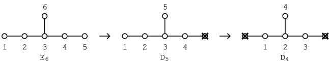
Figure 1: Dynkin diagrams

Removing a ${\bf C}$-brane induces the breaking of $SO(10)$ to $SO(8)\times U(1)$. Under $SO(8)\times U(1)$ the $SO(10)$ mass parameters are decomposed into the $SO(8)$ masses $c_{i}$ and $U(1)$ mass $M_{2}$ as follows:

$$b_{1}=M_{2},\hskip 28.45274ptb_{2}=M_{2}+c_{1},\hskip 28.45274ptb_{3}=M_{2}+c_{2},$$

$$b_{4}=M_{2}/2+c_{3},\hskip 28.45274ptb_{5}=M_{2}/2+c_{4}.$$ (6.2)

Upon sending ${\bf A}$- and ${\bf C}$-branes together to infinity we take the scaling limit [4]

$$M_{1},\;M_{2}\rightarrow\infty,\hskip 28.45274pt{M_{1}\over M_{2}}=-{\alpha+\beta\over 6(\alpha-\beta)}\quad{\rm fixed},$$ (6.3)

where the limit $M_{i}\rightarrow\infty$ decouples two $U(1)$ factors and the ratio with $\alpha,\,\beta$ defined in (2.11) gives the value of the marginal gauge coupling constant in the $D_{4}$ theory.

In order to see that the $E_{6}$ curve reduces to the $SO(8)$ SW curve (2.10) we first write the $E_{6}$ invariants $w_{q_{i}}(\phi)$ in terms of $SO(8)$ masses $c_{i}$

$$\phi_{1}=\frac{4}{3}(\alpha-2\beta)M,\hskip 19.91692pt\phi_{2}=\frac{2}{3}(\alpha-5\beta)M+c_{1},\hskip 19.91692pt\phi_{3}=-4\beta M+c_{2},$$

$$\phi_{4}=-\frac{2}{3}(\alpha+4\beta)+c_{3},\hskip 19.91692pt\phi_{5}=-\frac{4}{3}(\beta+\alpha)M,\hskip 19.91692pt\phi_{6}=-2\beta M+c_{4},$$ (6.4)

where $M=-3M_{1}/(\alpha+\beta)=M_{2}/(2(\alpha-\beta))$ and the explicit expressions of $w_{q_{i}}(\phi)$ in terms of $\phi_{i}$ are given in [32] . Then making a change of variables

$$y = -iM^{3}Y,$$

$$x = M^{2}\left(-X-\frac{1}{12}(\alpha-\beta)^{2}u_{2}+\frac{1}{3}(\alpha+\beta)Z\right),$$

$$z = \frac{2}{27}(\beta-2\alpha)(\alpha-2\beta)(\alpha+\beta)M^{3}+M\left(-\frac{1}{2}Z+\frac{1}{24}(\alpha+\beta)u_{2}\right)$$ (6.5)

in the $E_{6}$ curve and letting $M\rightarrow\infty$, we obtain the $SO(8)$ curve (2.10) where $m_{a}=m_{a}^{v}=(\lambda_{a},c)$ with $\lambda_{a}$ being a weight vector of ${\bf 8_{v}}$ in section 5.2.

We next show explicitly that, in the limit (6.3), the $E_{6}$ SW differential $\lambda_{\bf 27}^{E_{6}}$ in ${\bf 27}$ is reduced to the sum of the $D_{4}$ SW differentials in ${\bf 8_{v}},{\bf 8_{s}},{\bf 8_{c}}$ we have constructed previously. This corresponds to the fact that the fundamental representation ${\bf 27}$ of $E_{6}$ is decomposed under the $SO(8)$ subgroup into

$${\bf 27}={\bf 8_{v}}\oplus{\bf 8_{s}}\oplus{\bf 8_{c}}\oplus{\bf 1}\oplus{\bf 1}\oplus{\bf 1}.$$ (6.6)

Let us put (6.4), (6.5) in the $E_{6}$ differential (5.41)

$$\lambda^{E_{6}}_{\bf 27}=c_{2}\left(36z+\sum_{a=1}^{27}\frac{m_{a}(\phi_{i})y_{a}(z,\phi_{i})}{x-x_{a}(z,\phi_{i})}\right)\frac{dx}{y}.$$ (6.7)

and let $M\rightarrow\infty$, then we obtain

$$36z\frac{1}{i}\frac{dx}{y}=\left(-\frac{3}{8}(\alpha+\beta)(2\alpha-\beta)(2\beta-\alpha)M^{2}+18u-\frac{3}{2}(\alpha+\beta)u_{2}(c_{i})\right)\frac{dX}{Y}+O\left(\frac{1}{M}\right).$$ (6.8)

The poles in the singlets of $SO(8)$ go to infinity in this limit. Remember that the poles appear pairwise on two sheets of the Riemann surface in such a way that the sum of residues vanish. Indeed we have

$$\hskip 14.22636pt\sum_{a\in{\cal S}}\frac{1}{i}\frac{m_{a}y_{a}}{x-x_{a}}\frac{dx}{y}$$

$$=\left(\frac{3}{8}(\alpha+\beta)(2\alpha-\beta)(2\beta-\alpha)M^{2}-2Z+\frac{1}{6}(\alpha+\beta)u_{2}(c_{i})\right)\frac{dX}{Y}+O\left(\frac{1}{M}\right),$$ (6.9)

where ${\cal S}$ denotes a set of $SO(8)$ singlets, and hence the divergent pieces of (6.8) and (6.9) cancel out.

The pole terms in ${\bf 8_{v}}$ turn out to be

$$\frac{1}{i}\frac{m_{a}y_{a}}{x-x_{a}}\frac{dx}{y}=M\frac{A^{a}_{1}(Z,c_{i})+A^{a}_{2}(Z,c_{i})\frac{1}{M}+O\left(\frac{1}{M}\right)}{X-A^{a}_{3}(Z,c_{i})+A^{a}_{4}(Z,c_{i})\frac{1}{M}+O\left(\frac{1}{M}\right)}\frac{dX}{Y},$$ (6.10)

where $A^{a}_{i}$ is a polynomial of $Z$ and $c_{j}$. Although this seems to be divergent at first sight, the poles associated with weights $\lambda$ and $-\lambda$ in ${\bf 8_{v}}$ coalesce at the same point, making these contributions finite in the limit $M\rightarrow\infty$. It is verified that the sum over terms with these weights $\pm\lambda$ of ${\bf 8_{v}}$ becomes finite,

$$M\frac{A^{a}_{1}+A^{a}_{2}\frac{1}{M}+O\left(\frac{1}{M}\right)}{X-A^{a}_{3}+A^{a}_{4}\frac{1}{M}+O\left(\frac{1}{M}\right)}\frac{dX}{Y}+M\frac{-A^{a}_{1}+A^{a}_{2}\frac{1}{M}+O\left(\frac{1}{M}\right)}{X-A^{a}_{3}-A^{a}_{4}\frac{1}{M}+O\left(\frac{1}{M}\right)}\frac{dX}{Y}$$ (6.11)

$$= \frac{-2A^{a}_{1}A^{a}_{4}}{(X-A^{a}_{3})^{2}}\frac{dX}{Y}+\frac{2A^{a}_{2}}{X-A^{a}_{3}}\frac{dX}{Y}+O\left(\frac{1}{M}\right),$$

where we found that $A^{a}_{3}$ is equal to the pole position $X_{a}^{v}$ of $\lambda_{\bf 8_{v}}^{D_{4}}$. Thus we get

$$\sum_{a\in{\bf 8_{v}}}\frac{1}{i}\frac{m_{a}y_{a}}{x-x_{a}}\frac{dx}{y} \rightarrow \sum_{a=1}^{4}\left(\frac{-2A^{a}_{1}A^{a}_{4}}{(X-X^{v}_{a})^{2}}\frac{dX}{Y}+\frac{2A^{a}_{2}}{X-X^{v}_{a}}\frac{dX}{Y}\right)$$

$$= \sum_{a=1}^{4}\left(d\left(\frac{2A^{a}_{1}A^{a}_{4}}{X-X^{v}_{a}}\frac{1}{Y}\right)+\frac{A^{a}_{1}A^{a}_{4}}{X-X^{v}_{a}}\frac{1}{Y^{2}}\frac{\partial Y^{2}}{\partial X}\frac{dX}{Y}+\frac{2A^{a}_{2}}{X-X^{v}_{a}}\frac{dX}{Y}\right)$$

$$= \sum_{a=1}^{4}\left(\frac{1}{X-X^{v}_{a}}\frac{A^{a}_{1}A^{a}_{4}\frac{\partial Y^{2}}{\partial X}+2A_{2}^{a}Y^{2}}{Y^{2}}\frac{dX}{Y}+d\left(\frac{2A^{a}_{1}A^{a}_{4}}{X-X^{v}_{a}}\frac{1}{Y}\right)\right),$$

where the sum on the RHS is taken over half of the weights of ${\bf 8_{v}}$. We can proceed further by showing that

$$A^{a}_{1}(Z,c_{i})A^{a}_{4}(Z,c_{i})=-\gamma_{v}\,[Y^{2}]_{X=X^{v}_{a}}(Z,c_{i}),$$ (6.13)

and

$$\gamma_{v}\left[\frac{\partial Y^{2}}{\partial X}\right]_{X=X^{v}_{a}}-2A_{2}^{a}=2im^{v}_{a}\,\,[Y]_{X=X^{v}_{a}}(Z,c_{i}),$$ (6.14)

where $\gamma_{v}=\frac{\alpha+\beta}{3\alpha\beta}$.

Thus

$$\sum_{a\in{\bf 8_{v}}}\frac{1}{i}\frac{m_{a}y_{a}}{x-x_{a}}\frac{dx}{y}\rightarrow\sum_{a=1}^{4}\left(\frac{1}{i}\frac{2m^{v}_{a}[Y]_{X=X^{v}_{a}}}{X-X^{v}_{a}}\frac{dX}{Y}-d\left(\frac{2\gamma_{v}[Y^{2}]_{X=X^{v}_{a}}}{X-X^{v}_{a}}\frac{1}{Y}\right)-R^{v}_{a}\right),$$ (6.15)

where

$$R^{v}_{a}=\frac{\gamma_{v}}{Y^{2}}\frac{[Y^{2}]_{X=X^{v}_{a}}\frac{\partial Y^{2}}{\partial X}-Y^{2}\left[\frac{\partial Y^{2}}{\partial X}\right]_{X=X^{v}_{a}}}{X-X^{v}_{a}}\frac{dX}{Y}.$$ (6.16)

For the pole terms in ${\bf 8_{s}}$ of $SO(8)$ we obtain the result as in (6.15) except that we put $\alpha\rightarrow-\alpha$ and $\beta\rightarrow\beta-\alpha$ in $\gamma_{v}$ in (6.16) in accordance with the triality transformation and replace $X^{v}_{a}$ and $m_{a}^{v}$ by $X^{s}_{a}$ and $m^{s}_{a}$ for ${\bf 8_{s}}$ respectively. Likewise, for the pole terms in ${\bf 8_{c}}$ we let $X^{v}_{a}\rightarrow X^{v}_{c}$, $m_{a}^{v}\rightarrow m_{a}^{c}$ and $\beta\rightarrow-\beta$ and $\alpha\rightarrow\alpha-\beta$ in (6.15).

Finally we sum up the three pieces from ${\bf 8_{v}},{\bf 8_{s}},{\bf 8_{c}}$. In doing so, we observe that

$$\sum_{r=v,s,c}\sum_{a=1}^{4}R^{r}_{a}=P_{1}(Z,c_{i})\frac{dX}{Y}+2d\left(\frac{P_{1}(Z,c_{i})X-P_{2}(Z,c_{i})}{Y}\right),$$ (6.17)

where

$$P_{1} = 4Z-\frac{1}{3}(\alpha+\beta)u_{2}(c_{i}),$$

$$P_{2} = -\frac{2}{3}(\alpha+\beta)(\alpha^{2}-\alpha\beta+\beta^{2})u_{4}(c_{i})-2i(\alpha-\beta)(\alpha^{2}-\alpha\beta+\beta^{2})\widetilde{u}_{4}(c_{i})$$ (6.18)

$$\,\,+\frac{1}{12}(\alpha+\beta)^{3}{u_{2}(c_{i})}^{2}-\frac{4}{3}(\alpha^{2}-\alpha\beta+\beta^{2})u_{2}(c_{i})Z+\frac{4}{3}(\alpha+\beta)Z^{2}.$$

As a result, we find in the scaling limit that the $E_{6}$ SW differential in ${\bf 27}$ is reduced to the $SO(8)$ ones as

$$\lambda^{E_{6}}_{\bf 27} \rightarrow ic_{2}\left(12Z\frac{dX}{Y}-(\alpha+\beta)u_{2}(c_{i})\frac{dX}{Y}+2\sum_{r=v,s,c}\sum_{a=1}^{4}\frac{1}{i}\frac{m^{r}_{a}[Y]_{X=X^{r}_{a}}}{X-X^{r}_{a}}\frac{dX}{Y}\right)+d(*)$$ (6.19)

$$= 8\pi\sqrt{2}ic_{2}\left(\lambda^{\bf 8_{v}}_{SW}+\lambda^{\bf 8_{s}}_{SW}+\lambda^{\bf 8_{c}}_{SW}\right)+d(*),$$

where $\lambda^{\bf 8_{\bullet}}_{SW}$ has been normalized as in (5.38).

We encounter here a somewhat curious situation; $\lambda_{\bf 27}^{E_{6}}$ does not reduce to one of the $\lambda^{\bf 8_{\bullet}}_{SW}$, but the sum of $\lambda^{\bf 8_{\bullet}}_{SW}$. In view of (6.6) and $SO(8)$ triality, on the one hand, (6.19) seems natural. Then one would say that picking up any one of $\lambda^{\bf 8_{\bullet}}_{SW}$ is sufficient to describe the physics. Note, however, that the location of poles and their residues depend on ${\bf 8_{v}},{\bf 8_{s}},{\bf 8_{c}}$, and it is not so obvious if the irrelevance of which ${\bf 8}$ of $SO(8)$ we choose to construct the SW differential is really due to triality invariance which is inherent in $SO(8)$. In addition to this, the SW differential $\lambda_{\bf 78}^{E_{6}}$ looks totally different from $\lambda_{\bf 27}^{E_{6}}$. This is also the case in the $D_{4}$ theory. In what follows we will study if the representation chosen in constructing $\lambda$ is relevant to the physics or not.

7 Universality of Seiberg-Witten periods

Having derived (6.19), how do we fix the normalization constant $c_{2}$ for $\lambda_{\bf 27}^{E_{6}}$? Let us first point out that, under the renormalization group flows (2.2), the period integrals

$$\oint{\partial\lambda_{\cal R}^{G}\over\partial z}$$ (7.1)

exhibit the smooth limiting behavior at the generic points on the moduli space. Then we obtain from (5.42) and (6.5) that $c_{2}={\sqrt{2}\over 48\pi i}$ for $\lambda_{\bf 27}^{E_{6}}$. Eq.(6.19) is written as

$$\lambda_{\bf 27}^{E_{6}}\rightarrow{1\over 3}\left(\lambda^{\bf 8_{v}}_{SW}+\lambda^{\bf 8_{s}}_{SW}+\lambda^{\bf 8_{c}}_{SW}\right)+d(*).$$ (7.2)

We also observe that the residues of the poles of $\lambda_{\bf 27}^{E_{6}}$ turn out to be

$$2\pi i{\rm Res}_{x=x_{a}}(\lambda_{\bf 27}^{E_{6}})=\frac{1}{k_{\bf 27}}\frac{m_{a}}{2\sqrt{2}}$$ (7.3)

with $k_{\bf 27}=6$. Notice that the index of ${\bf 27}$ (or ${\bf\overline{27}}$) is equal to 6. The appearance of the index of representations is not peculiar to this case. For example, in (5.49) and (5.52) we see $12=\ell({\bf 56})$ and $36=\ell({\bf 133})$, respectively, where $\ell({\cal R})$ is the index of the representation ${\cal R}$ (see Table 3).

	index
$A_{1}$	$\ell({\bf 3})=4$	$\ell({\bf 2})=1$
$A_{2}$	$\ell({\bf 8})=6$	$\ell({\bf 3})=\ell({\bf\bar{3}})=1$
$D_{4}$	$\ell({\bf 28})=12$	$\ell({\bf 8_{v}})=\ell({\bf 8_{s}})=\ell({\bf 8_{c}})=2$
$E_{6}$	$\ell({\bf 78})=24$	$\ell({\bf 27})=\ell({\bf\overline{27}})=6$
$E_{7}$	$\ell({\bf 133})=36$	$\ell({\bf 56})=12$
$E_{8}$	$\ell({\bf 248})=60$

Table 3: Index of representations. $\ell$(adjoint)$=2h$ and $\ell({\bf 1})=0$.

Now examining the SW differentials obtained for various instances in section 5 and the renormalization group flows (see also [5, 6, 8]), we find that the residue should be normalized as

$$2\pi i{\rm Res}_{x=x_{a}}(\lambda_{\cal R}^{G})=\frac{1}{k_{\cal R}}\frac{m_{a}}{2\sqrt{2}},\hskip 28.45274ptm_{a}=(\lambda_{a},\phi),$$ (7.4)

where $k_{\cal R}=\ell({\cal R})$, or $k_{\cal R}=\ell({\cal R})/2$ if the sum of the poles is taken over half of the (non-zero) weights of ${\cal R}$, and we use $\lambda_{SW}^{\cal R}$ for the $D_{4}$ differential. Here the mass parameter $\phi$ is normalized so that we have $m_{a}^{v}=(\lambda_{a},\phi)$ in the $D_{4}$ theory along the flows (2.2). This explains why we need to be a little careful to fix a numerical constant upon relating $m_{a}$ and $v_{a}$ in section 5. With this normalization of residues, it can be checked that the two-form $\Omega$ in (4.1) is invariant under the successive flows (2.2). We also see that

$${\partial\lambda_{\cal R}^{G}\over\partial z}=\kappa_{G}{dx\over y},$$ (7.5)

where $\kappa_{G}$ is independent of ${\cal R}$ as read off from section 5.

We claim that (7.4) is the correct normalization of the residue. Taking this for granted, consider the renormalization group flow from the $G$ theory to the $G^{\prime}$ theory. In the $G$ theory, let the residues of the SW differential transform in the representation ${\cal R}$ of $G$. If the ${\cal R}$ branches to $\oplus_{i}{\cal R}^{\prime}_{i}$ under $G\supset G^{\prime}$, the pole terms of $\lambda^{G}_{\cal R}$ reduce to the sum of pole terms each of which transforms in ${\cal R}^{\prime}_{i}$ of $G^{\prime}$. As observed in the flow $E_{6}\rightarrow D_{4}$ we expect that the pole terms belonging to non-singlets of $G^{\prime}$ remain finite in the scaling limit which implements the flow $G\rightarrow G^{\prime}$. If this is assumed to be the case, we obtain

$$\lambda^{G}_{\cal R}\longrightarrow\sum_{{\cal R}^{\prime}_{i}\not={\bf 1}}{\ell({\cal R}^{\prime}_{i})\over\ell({\cal R})}\lambda^{G^{\prime}}_{{\cal R}^{\prime}_{i}}+d(*)$$ (7.6)

by matching the normalization of residues. This behavior is actually observed in (6.19).

7.1 Irrelevance of representations

For a branching ${\cal R}=\oplus_{i}{\cal R}^{\prime}_{i}$, we recall the identity $\ell({\cal R})=\sum_{i}\ell({\cal R}^{\prime}_{i})$. Then (7.6) may imply that the period integrals of $\lambda^{G^{\prime}}_{{\cal R}^{\prime}_{i}}$ are independent of ${\cal R}^{\prime}_{i}$. This may sound surprising, but we now prove that the SW differentials in any representation yield the identical physics result.

Since $\lambda^{G}_{{\cal R}}$ has the poles with nonzero residues, there is ambiguity in evaluating the periods if we specify the cycles, along which $\lambda^{G}_{{\cal R}}$ is integrated, only in terms of the homology class of the SW curve. Thus we consider the SW curve as the torus with punctures at the location of the poles of $\lambda^{G}_{{\cal R}}$. The homology class of this punctured torus has a basis $\alpha$, $\beta$ and $\gamma_{a}$. Here $\gamma_{a}$ goes around a pole at $x=x_{a}$ counterclockwise, and the cycles $\alpha$ and $\beta$ will be specified later.

Given $\lambda^{G}_{{\cal R}_{j}}$ in the representation ${\cal R}_{j}$, we define

$$a_{{\cal R}_{j}}(z,\phi)=\oint_{\alpha}\lambda^{G}_{{\cal R}_{j}},\hskip 28.45274pt{a_{D}}_{{\cal R}_{j}}(z,\phi)=\int_{\beta}\lambda^{G}_{{\cal R}_{j}}$$ (7.7)

and

$$f(z,\phi)=a_{{\cal R}_{1}}-a_{{\cal R}_{2}},\hskip 28.45274ptf_{D}(z,\phi)={a_{D}}_{{\cal R}_{1}}-{a_{D}}_{{\cal R}_{2}}.$$ (7.8)

It is an immediate consequence of (7.5) that $f(z,m)=f(m)$ and $f_{D}(z,m)=f_{D}(m)$. When we loop around a singularity at $z=z_{k}$ on the $z$-plane, $\lambda_{\cal R}^{G}$ remains invariant but the cycles undergo the monodromy

$$\alpha \rightarrow n\alpha+m\beta+\sum_{a}l_{a}\gamma_{a},$$

$$\beta \rightarrow n^{\prime}\alpha+m^{\prime}\beta+\sum_{a}l^{\prime}_{a}\gamma_{a},$$ (7.9)

where the matrix $\pmatrix{n&m\cr n^{\prime}&m^{\prime}\cr}$ is conjugate to $T=\pmatrix{1&1\cr 0&1\cr}$ and $l,\,l^{\prime}$ are some integers which are non-zero when a cycle crosses a pole under a monodromy transformation. At the singularity $z=z_{k}$, therefore, we have a linear relation among $a_{{\cal R}_{j}}$, ${a_{D}}_{{\cal R}_{j}}$ and ${\rm Res}(\lambda^{G}_{{\cal R}_{j}})$. This in turn gives rise to a linear relation for $f(m)$, $f_{D}(m)$ and the residues. A similar consideration at different singularity, say at $z=z_{k^{\prime}}$, yields another linear relation. These two relations are linearly independent when two 7-branes at $z=z_{k}$ and at $z=z_{k^{\prime}}$ are mutually non-local. Then we find

$$f(m)=\sum_{j=1}^{2}\sum_{a_{j}}c_{a_{j}}{\rm Res}_{x=x_{a_{j}}}(\lambda^{G}_{{\cal R}_{j}}),\hskip 28.45274ptf_{D}(m)=\sum_{j=1}^{2}\sum_{a_{j}}c^{\prime}_{a_{j}}{\rm Res}_{x=x_{a_{j}}}(\lambda^{G}_{{\cal R}_{j}}),$$ (7.10)

where $c_{a_{j}},\,c^{\prime}_{a_{j}}$ are some constants. Hence we have shown that $f(m)$ and $f_{D}(m)$ are linear in $m_{a}$. In fact, if $f(m)$ were not linear in $m_{a}$, then for every $z$, we could have taken $1/f(m)=0$ in the codimension one subspace of the space of bare mass parameters. For a generic value of $z$, however, $f(m)$ may not be divergent, and hence $f(m)$ should be linear in $m$.

Let us now apply a Weyl transformations $m_{a}\rightarrow\widetilde{m}_{a}$ under which $\lambda^{G}_{R_{i}}$ is left invariant. The SW periods $a(z,m)$ and $a_{D}(z,m)$, however, may exhibit a non-trivial behavior under the Weyl reflection. This occurs if the Weyl reflection moves a pole of $\lambda_{\cal R}^{G}$ on the $x$-plane across the $\alpha$ and/or $\beta$ cycles. The SW periods, on the other hand, should be Weyl invariant as gauge invariant expectation values. We thus prescribe that the positions of the cycles $\alpha$ and $\beta$ are fixed relatively to the poles in such a way that the relative positions of the cycles and the poles do not change under a Weyl transformation. Since it is always possible to take such $\alpha$ and $\beta$ in the asymptotic region $z\gg m_{a}$ of the moduli space, we henceforth specify the cycles according to this prescription. As a consequence of this, we see that $f(m)=f(\widetilde{m})$ and $f_{D}(m)=f_{D}(\widetilde{m})$. Remember here the fact that there are no Weyl invariants which are linear in $m_{a}$, and hence we obtain $f(m)=f_{D}(m)=0$. Therefore, we conclude that the SW periods $a,\,a_{D}$ are independent of the choice of a representation in constructing $\lambda_{\cal R}^{G}$ as long as the cycles $\alpha,\,\beta$ are fixed properly as described above.

7.2 Numerical check

One can numerically evaluate the period integrals and check that $a$ and $a_{D}$ are independent of the representation ${\cal R}$ of the residues of $\lambda^{G}_{\cal R}$. In the case of $A_{2}$ and $D_{4}$, we express $a_{\cal R}$ and ${a_{D}}_{\cal R}$ for ${\cal R}=f$(undamental) and $adj$(oint) in terms of standard elliptic integrals by taking two cycles $\alpha,\,\beta$ as we prescribed above. With the use of Maple, we then obtain, for example, $a_{f}=-28.99673387+16.74790178\,i$ and $a_{adj}=-28.99673386+16.74790178\,i$ in the $A_{2}$ theory at $z=10$, $m_{1}=1-0.2\,i$ and $m_{2}=-0.4+0.75\,i$. The error is indeed extremely small compared to the ratio of $z$ to $m_{i}$. Varying the values of $m_{i}$ we plot in Fig.2 the real and imaginary parts of $a_{f}$ in the $A_{2}$ theory for $z=10$ and $m_{1}=2x-0.2\,i,\;m_{2}=-0.4+1.5\,i\,x$. Computing the periods at various values of $z$ and $m_{i}$, we have observed in both $A_{2}$ and $D_{4}$ theories that

$$\frac{a_{f}-a_{adj}}{a_{f}}<10^{-8},\hskip 28.45274pt\frac{{a_{D}}_{f}-{a_{D}}_{adj}}{{a_{D}}_{f}}<10^{-8},$$ (7.11)

where the differentials (5.26), (5.31) have been utilized in the $D_{4}$ theory. Since the values of $a$ and $a_{D}$ change substantially as shown in Fig.2 upon varying parameters of the moduli space, we believe that the RHS of (7.11) are numerical errors and really mean zero.

Figure 2: The period $a=\int_{\alpha}\lambda^{A_{2}}_{f}$ in the fundamental of $SU(3)$ is plotted for $z=10,\;m_{1}=2x-0.2\,i,\;m_{2}=-0.4+1.5\,i\,x$ .

To summarize, the SW periods will jump by a constant given by the residue of $\lambda_{\cal R}^{G}$ if we continuously deform the $\alpha,\,\beta$ cycles across a pole. Namely, the dependence of the periods on the cycles cannot be absorbed by the redefinition of the periods among themselves. Furthermore, since the positions of the poles and their residues are solely determined by the representation ${\cal R}$ chosen to construct $\lambda_{\cal R}^{G}$, how to fix the location of the cycles relatively to the poles is a subtle issue. In spite of these, we have prescribed a way of specifying the cycles, based on which the irrelevance of representations to the SW periods is proved. To fix the BPS central charge, it remains to determine the constant piece of the global abelian charges as mentioned in section 3. This will be possible once we locate the cycles along which $\lambda_{\cal R}^{G}$ is integrated. It is also important to study the monodromy properties explicitly toward a full account of the BPS spectrum.

8 Flows to $N=2$ $SU(2)$ QCD with $N_{f}\leq 3$

It is well known that in $N=2$ $SU(2)$ QCD with $N_{f}$ fundamental quarks, the global symmetry is enhanced to $SO(2N_{f})$ when the quarks are massless [6]. We now analyze how the SW differentials in the $N_{f}=4$ theory reduce to those in $N_{f}<4$ theories.

8.1 Vector representation

Let us first take the $N_{f}=4$ SW differential $\lambda_{SW}^{\bf 8_{v}}$ in the vector representation of $SO(8)$. Upon taking the scaling limit $\alpha\beta\rightarrow 1,\;\alpha+\beta\rightarrow-2$ and $m_{4}\rightarrow\infty$ with $(\alpha-\beta)m_{4}=-\Lambda_{3}/4$ fixed [6], we obtain the $N_{f}=3$ theory. In this limit the $D_{4}$ curve (2.10), which can be rewritten as

$$Y^{2}=\alpha\beta X\left(Z-\frac{(\alpha-\beta)\alpha^{2}\beta^{2}\prod_{b=1}^{4}m_{b}+(\alpha+\beta)X^{2}}{2\alpha\beta X}\right)^{2}-\frac{(\alpha-\beta)^{2}}{4\alpha\beta X}\prod_{a=1}^{4}(X+\alpha\beta m_{a}^{2}),$$ (8.1)

becomes

$$Y^{2}=X\left(X+Z+\frac{m_{1}m_{2}m_{3}\Lambda_{3}}{8X}\right)^{2}-\frac{\Lambda^{2}}{64X}\prod_{a=1}^{3}(X+m_{a}^{2}).$$ (8.2)

This is shown to be equivalent to the usual $N_{f}=3$ curve by setting $X=X^{\prime}-Z$

$$Y^{2} = X^{\prime 2}(X^{\prime}-Z)-\frac{\Lambda_{3}^{2}}{64}(X^{\prime}-Z)^{2}-\frac{\Lambda_{3}^{2}}{64}(m_{1}^{2}+m_{2}^{2}+m_{3}^{2})(X^{\prime}-Z)$$ (8.3)

$$+\frac{\Lambda_{3}}{4}m_{1}m_{2}m_{3}X^{\prime}-\frac{\Lambda_{3}^{2}}{64}(m_{1}^{2}\,m_{2}^{2}+m_{2}^{2}\,m_{3}^{2}+m_{1}^{2}\,m_{3}^{2}).$$

Turning to the differential, one can verify that $\lambda_{SW}^{\bf 8_{v}}$ in (5.35) with $X_{a}^{v}=-\alpha\beta m_{a}^{2}$ and

$$Y_{a}=-i\alpha\beta m_{a}\left(Z+\frac{(\alpha-\beta)\alpha^{2}\beta^{2}\prod_{a=1}^{4}m_{a}+(\alpha+\beta)\alpha^{2}\beta^{2}m_{a}^{4}}{2\alpha^{2}\beta^{2}m_{a}^{2}}\right),$$ (8.4)

yields the $N_{f}=3$ SW differential

$$\lambda_{D_{3}}^{\bf 6_{v}}=\frac{\sqrt{2}}{8\pi}\left(2Z-X^{\prime}-(m_{1}^{2}+m_{2}^{2}+m_{3}^{2})\right)\frac{dX^{\prime}}{Y}-\frac{\sqrt{2}}{8\pi}\sum_{a=1}^{3}\frac{m_{a}^{2}Z-\frac{1}{8}m_{1}m_{2}m_{3}\Lambda_{3}-m_{a}^{4}}{X^{\prime}-Z+m_{a}^{2}}\frac{dX^{\prime}}{Y}$$ (8.5)

which corresponds to the vector representation of $SO(6)$.

Taking here the limit $m_{3}\rightarrow\infty$ with $\Lambda_{3}m_{3}=\Lambda_{2}^{2}$ fixed, we have the $N_{f}=2$ theory with the curve

$$Y^{2}=X^{\prime 2}(X^{\prime}-Z)-\frac{\Lambda_{2}^{2}}{64}(X^{\prime}-Z)+{\Lambda_{2}^{2}\over 4}m_{1}m_{2}X^{\prime}-{\Lambda_{2}^{4}\over 64}(m_{1}^{2}+m_{2}^{2}).$$ (8.6)

The SW differential obtained from (8.5) turns out to be

$$\lambda_{D_{2}}^{\bf 4_{v}}=\frac{\sqrt{2}}{8\pi}\left(2Z-2X^{\prime}-(m_{1}^{2}+m_{2}^{2})\right)\frac{dX^{\prime}}{Y}-\frac{\sqrt{2}}{8\pi}\sum_{a=1}^{2}\frac{m_{a}^{2}Z-\frac{1}{8}m_{1}m_{2}\Lambda_{2}^{2}-m_{a}^{4}}{X^{\prime}-Z+m_{a}^{2}}\frac{dX^{\prime}}{Y}.$$ (8.7)

Next, in the limit $m_{2}\rightarrow\infty$ with $\Lambda_{2}^{2}m_{2}=\Lambda_{1}^{3}$ fixed, we obtain the $N_{f}=1$ curve from (8.6)

$$Y^{2}=X^{\prime 2}(X^{\prime}-Z)+{\Lambda_{1}^{3}\over 4}m_{1}X^{\prime}-{\Lambda_{1}^{6}\over 64}$$ (8.8)

and the differential

$$\lambda_{D_{1}}^{\bf 2_{v}}=\frac{\sqrt{2}}{8\pi}\left(2Z-3X^{\prime}-m_{1}^{2}\right)\frac{dX^{\prime}}{Y}-\frac{\sqrt{2}}{8\pi}\frac{m_{1}^{2}Z-\frac{1}{8}m_{1}\Lambda_{1}^{3}-m_{1}^{4}}{X^{\prime}-Z+m_{1}^{2}}\frac{dX^{\prime}}{Y}.$$ (8.9)

Finally, letting $m_{1}\rightarrow\infty$ with $\Lambda_{1}^{3}m_{1}=\Lambda_{0}^{4}$ fixed, we arrive at the $N_{f}=0$ theory with the curve

$$Y^{2}=X^{\prime 2}(X^{\prime}-Z)+{\Lambda_{0}^{4}\over 4}X^{\prime}$$ (8.10)

and the standard form of the differential

$$\lambda_{YM}=\frac{\sqrt{2}}{8\pi}\left(2Z-4X^{\prime}\right)\frac{dX^{\prime}}{Y}.$$ (8.11)

Thus, under these renormalization group flows, we obtain the SW differentials in the vector representation of $SO(2N_{f})$.

We see from the above that the residues of $\lambda_{D_{n}}^{\bf{2n}_{v}}$ read

$$2\pi i{\rm Res}\left(\lambda_{D_{n}}^{\bf{2n}_{v}}\right)={m_{a}\over 2\sqrt{2}}$$ (8.12)

for $n\leq 4$, which agrees with (7.4) because $k_{\bf{2n}_{v}}=1$, but differs from (17.1) of [6]. The present result is the correct one since $\lambda_{YM}$ derived through the successive flows from $D_{4}$ coincides with that obtained in [33]. In order for this to hold, it is important that $\lambda_{D_{n}}^{\bf{2n}_{v}}$ obeys

$$\frac{\partial\lambda_{D_{n}}^{\bf{2n}_{v}}}{\partial Z}=\frac{\sqrt{2}}{8\pi}\frac{dX^{\prime}}{Y}.$$ (8.13)

Furthermore it is clear that the massless limit of $\lambda_{D_{n}}^{\bf 2n_{v}}$ is in agreement with the ones obtained in [33].

8.2 Spinor representation

One may notice that the differentials $\lambda_{D_{n}}^{\bf 2n_{v}}$ do not look like those obtained in [6, 34, 23]. Our next task is to show that they are indeed derived from the $N_{f}=4$ SW differentials in spinors of $SO(8)$ and their residues transform in the spinor representation of $SO(2N_{f})$ with $N_{f}\leq 3$.

First of all we note that the weights of ${\bf 8_{s}}$ of $SO(8)$ are given by

$$m_{1}^{s}=\frac{1}{2}(m_{1}+m_{2}+m_{3}+m_{4}),$$

$$m_{2}^{s}=\frac{1}{2}(m_{1}+m_{2}-m_{3}-m_{4}),$$

$$m_{3}^{s}=\frac{1}{2}(m_{1}-m_{2}+m_{3}-m_{4}),$$

$$m_{4}^{s}=\frac{1}{2}(m_{1}-m_{2}-m_{3}+m_{4})$$ (8.14)

and $m_{4+a}^{s}=-m_{a}^{s}$. Note also $u_{2}=-\sum_{a=1}^{4}m_{a}^{2}=-\sum_{a=1}^{4}(m_{a}^{s})^{2}$. In $\lambda_{SW}^{\bf 8_{s}}$ (5.27), one has $X_{a}^{s}=\alpha Z-\alpha(\alpha-\beta)(\frac{1}{4}u_{2}+(m_{a}^{s})^{2})$. Under the flow $D_{4}\rightarrow D_{3}$ generated by taking the scaling limit $m_{4}\rightarrow\infty$, ${\bf 8_{s}}$ of $SO(8)$ is reduced to ${\bf 4_{s}}+{\bf 4_{c}}$ of $SO(6)$ where the weights of ${\bf 4_{s}}$ are

$$m_{1}^{\bf 4_{s}}=(m_{1}+m_{2}+m_{3})/2,\hskip 36.98857ptm_{2}^{\bf 4_{s}}=-(m_{1}+m_{2}-m_{3})/2,$$

$$m_{3}^{\bf 4_{s}}=-(m_{1}-m_{2}+m_{3})/2,\hskip 28.45274ptm_{4}^{\bf 4_{s}}=(m_{1}-m_{2}-m_{3})/2$$ (8.15)

and the weights of ${\bf 4_{c}}$ are $m_{a}^{\bf 4_{c}}=-m_{a}^{\bf 4_{s}}$. The positions $X_{a}^{s}$ of the poles become

$$X_{a}^{s} = -Z-\frac{1}{4}m_{a}^{\bf 4_{s}}\Lambda_{3}$$

$$-\frac{1}{m_{4}}\Biggl{(}\frac{1}{32}m_{a}^{\bf 4_{s}}\Lambda_{3}^{2}+\frac{1}{8}Z\Lambda_{3}+\frac{1}{16}\Lambda_{3}\left(-\sum_{b=1}^{4}(m_{b}^{\bf 4_{s}})^{2}+4(m_{a}^{\bf 4_{s}})^{2}\right)\Biggr{)}+O\left(\frac{1}{m_{4}^{2}}\right),$$

from which we see that the poles are not sent to infinity. On the other hand, the residue is evidently divergent. This gives rise to a divergent piece in the SW periods in the scaling limit $m_{4}\rightarrow\infty$. We note that this is a necessary divergence to make certain BPS states decouple. To avoid this divergent behavior, though harmless, let us alternatively take the differential $\frac{1}{2}(\lambda_{SW}^{\bf 8_{s}}+\lambda_{SW}^{\bf 8_{c}})$. For this combination, we can evaluate the limit as performed in the flow from $E_{6}$ to $D_{4}$. The result is

$$\frac{1}{2}(\lambda_{SW}^{\bf 8_{s}}+\lambda_{SW}^{\bf 8_{c}})\rightarrow\lambda_{D_{3}}^{\bf 4_{s}}+dF(X^{\prime},Z,m_{a}^{\bf 4_{s}}),$$ (8.17)

where

$$\lambda_{D_{3}}^{\bf 4_{s}}=\frac{\sqrt{2}}{8\pi}\left(2Z-X^{\prime}\right)\frac{dX^{\prime}}{Y}-\frac{\sqrt{2}}{8\pi}\sum_{a=1}^{4}\frac{m_{a}^{\bf 4_{s}}\frac{\Lambda_{3}}{32}(4Z-2\sum_{b=1}^{4}(m_{b}^{\bf 4_{s}})^{2}+8(m_{a}^{\bf 4_{s}})^{2}+\Lambda_{3}m_{a}^{\bf 4_{s}})}{X^{\prime}+\frac{1}{4}m_{a}^{\bf 4_{s}}\Lambda_{3}}\frac{dX^{\prime}}{Y}$$ (8.18)

and

$$F=\frac{\sqrt{2}}{256\pi}\frac{1}{Y}\Biggl{(}64X^{\prime 2}-64(Z+\Lambda_{3}^{2})X^{\prime}+16m_{1}m_{2}m_{3}\Lambda_{3}$$

$$\hskip 85.35826pt+2Z\Lambda_{3}^{2}+64\sum_{a=1}^{4}\frac{[Y]_{X^{\prime}=-\frac{1}{4}m_{a}^{\bf 4_{s}}\Lambda_{3}}}{X^{\prime}+\frac{1}{4}m_{a}^{\bf 4_{s}}\Lambda_{3}}\Biggr{)}.$$ (8.19)

The differential (8.18) for the $N_{f}=3$ theory indeed agrees with [34] and has the poles with residues in the form of (7.4) since the index of ${\bf 4_{s}}$ of $SO(6)$ is 1.

Next, taking the limit $m_{3}\rightarrow\infty$ with $\Lambda_{3}m_{3}=\Lambda_{2}^{2}$ fixed to have the $N_{f}=2$ theory, it is shown that

$$\lambda_{D_{3}}^{\bf 4_{s}}\rightarrow\lambda_{D_{2}}^{{\bf 2_{L}}{\bf 2_{R}}}+d\left(\sqrt{2}\,\frac{4X^{\prime 2}-4ZX^{\prime}+m_{1}m_{2}\Lambda_{2}^{2}}{8\pi Y}+\frac{\sqrt{2}}{2\pi}\sum_{a=1}^{2}\frac{[Y]_{X^{\prime}=-\frac{1}{8}\Lambda_{2}^{2}}}{X^{\prime}+\frac{1}{8}\Lambda_{2}^{2}}\frac{1}{Y}\right),$$ (8.20)

where

$$\lambda_{D_{2}}^{{\bf 2_{L}}{\bf 2_{R}}} = \frac{\sqrt{2}}{4\pi}\left(Z-X^{\prime}\right)\frac{dX^{\prime}}{Y}-\frac{\sqrt{2}}{4\pi}\left(\frac{m^{\bf 2_{L}}\frac{\Lambda_{2}^{2}}{4}m^{\bf 2_{L}}}{X^{\prime}+\frac{1}{8}\Lambda_{2}^{2}}-\frac{m^{\bf 2_{R}}\frac{\Lambda_{2}^{2}}{4}m^{\bf 2_{R}}}{X^{\prime}-\frac{1}{8}\Lambda_{2}^{2}}\right)\frac{dX^{\prime}}{Y}$$ (8.21)

$$= \frac{-\sqrt{2}}{4\pi}\frac{YdX^{\prime}}{X^{\prime 2}-\frac{1}{64}\Lambda_{2}^{4}},$$

which is in agreement with the one obtained in [6]. Here ${\bf 4_{s}}$ of $SO(6)$ is decomposed into $({\bf 2},{\bf 1})+({\bf 1},{\bf 2})$ of $SU(2)\times SU(2)\,(=Spin(4))$ and the corresponding highest weights are given by $m^{\bf 2_{R}}=(m_{1}+m_{2})/2$ and $m^{\bf 2_{L}}=(m_{1}-m_{2})/2$. Thus the residues of $\lambda_{D_{2}}^{{\bf 2_{L}}{\bf 2_{R}}}$ read off from (8.21) become ${1\over 2\pi i}{m_{1}\pm m_{2}\over 2\sqrt{2}}$, which is the well-known result [6].

In the limit $m_{2}\rightarrow\infty$ with $\Lambda_{2}^{2}m_{2}=\Lambda_{1}^{3}$ fixed, we find the differential for the $N_{f}=1$ theory

$$\lambda_{D_{2}}^{\bf 2_{s}}\rightarrow\lambda_{D_{1}}^{\bf 1_{s}}+d\left(\sqrt{2}\,\frac{-2X^{\prime 2}+2ZX^{\prime}-m_{1}\Lambda_{1}^{3}-\Lambda_{1}^{6}/x}{8\pi Y}\right),$$ (8.22)

where

$$\lambda_{D_{1}}^{\bf 1_{s}}=\frac{\sqrt{2}}{8\pi}\left(2Z-3X^{\prime}\right)\frac{dX^{\prime}}{Y}-\frac{\sqrt{2}}{8\pi}\frac{m_{1}\Lambda_{1}^{3}}{4X^{\prime}}\frac{dX^{\prime}}{Y}$$ (8.23)

which again agrees with [34, 23].

Finally, we let $m_{1}\rightarrow\infty$ with $\Lambda_{1}^{3}m_{1}=\Lambda_{0}^{4}$ fixed to obtain the $N_{f}=0$ theory. In this limit we see that the pole at $X^{\prime}=0$ in (8.23) turns out to be a double pole. Then, using the $N_{f}=0$ curve $\frac{1}{X^{\prime}}={1\over Y^{2}}(X^{\prime 2}-ZX^{\prime}+\frac{1}{4}\Lambda_{0}^{4})$, we arrive at

$$\lambda_{D_{1}}^{\bf 1_{s}}\rightarrow\lambda_{YM}-\frac{\sqrt{2}}{8\pi}d\left(\frac{-4X^{\prime 2}+4ZX^{\prime}-\Lambda_{0}^{4}}{2Y}\right).$$ (8.24)

In this section, we have shown that the SW differentials in the $N_{f}\leq 3$ theories can be built from the vector as well as spinor representations of $SO(2N_{f})$. According to section 7 they describe the same physics in the Coulomb branch of $N=2$ $SU(2)$ QCD with massive quarks. The SW differentials for $N_{f}\leq 3$ in general take the form

$$\lambda_{D_{N_{f}}}^{\cal R}={\sqrt{2}\over 8\pi}\left(2Z-(4-N_{f})X^{\prime}\right){dX^{\prime}\over Y}+(\hbox{pole terms}).$$ (8.25)

Note here that $X^{\prime}dX^{\prime}/Y$ has double poles at infinity whose existence is characteristic of the asymptotic freedom. It is interesting that simple poles of $\lambda_{D_{N_{f}}}^{\cal R}$ due to a massive quark become congruent to the double poles at infinity in the scaling limit $N_{f}\rightarrow N_{f}-1$.

9 Conclusions

In the framework of the F-theory compactification, we have written down the elliptic curves for describing the $N=2$ theories with $ADE$ global symmetries on a D3-brane in the Type IIB 7-brane background. The SW differentials $\lambda$ have then been constructed for the fundamental and adjoint representations of the $ADE$ groups. It is shown that the physics results are independent of the representation of $\lambda$. It is interesting to compare the present result with what has been known in four-dimensional $N=2$ Yang-Mills theory with $ADE$ gauge symmetries. For $N=2$ $ADE$ Yang-Mills theory the SW curves are given by the spectral curves whose form depends explicitly on the representations ${\cal R}$ of $ADE$. However, the physics of the Coulomb branch is equally described irrespective of ${\cal R}$. In [35] this is shown in terms of the universality of the special Prym variety known in the theory of spectral curves [36]. This is seen more explicitly by analyzing the Picard-Fuchs equations for the SW periods [28]. Therefore, the universality we found here is considered as the global symmetry version of the universality in $N=2$ Yang-Mills theory with local $ADE$ gauge symmetries.

It is clear in the framework of Type II string theory that the $ADE$ global symmetries on a D3-brane and the $ADE$ gauge symmetries of four-dimensional Yang-Mills theory have the common origin in the $ADE$ singularities appearing in the degeneration of a $K3$ surface. In fact, if we replace the top Casimir $w_{h}$ by $w_{h}+\rho+\Lambda^{2h}/\rho$ in (2.4)-(2.9), our $ADE$ curves are recognized as the equations for the $ADE$ ALE space fibered over ${\bf P}^{1}$. Here $\rho$ is a complex coordinate of the base ${\bf P}^{1}$. This reflects the compactification of Type II string theory on a $K3$ fibered Calabi-Yau threefold. From this point of view, our calculation for the fundamental of $E_{6}$ in section 5.3 is indeed equivalent to that in [37] to obtain the SW curve for the $N=2$ $E_{6}$ Yang-Mills theory from the fibration of the $E_{6}$ ALE space. Hence our computations in section 5 can be viewed as the determination of the SW curves in the fundamental and adjoint representations for $N=2$ Yang-Mills theory with $ADE$ gauge symmetries.

The global sections of an elliptic fibration in higher representations than the adjoint may be found by constructing the meromorphic sections. The lattice structure hidden in our explicit computations will be related to the lattice which arises in the Mordell-Weil group. It will be interesting to formulate our present results in more precise mathematical terms in view of the relation between the Mordell-Weil lattice and the $ADE$ singularity theory.

Finally, it is very interesting to analyze the BPS spectrum of the $E_{n}$ theories using our results. One application is to construct the junction lattice explicitly to describe the BPS states. This can be done at least numerically as has been performed in $N=2$ $SU(2)$ theory [38, 39]. In the $E_{n}$ theories the BPS spectrum possesses the rich structure in comparison with the $D_{n\leq 4}$ theories [11]. For instance, BPS states in arbitrary higher representations of the $E_{n}$ groups are shown to exist on the basis of (3.2). Combining the SW description properly formulated in the present paper and the junction approach will be efficient to gain a deeper understanding of still mysterious four-dimensional $N=2$ superconformal field theories with exceptional symmetry.

Acknowledgements

We are grateful to K. Mohri, S. Sugimoto and Y. Yamada for useful discussions. One of us (SKY) would like to thank T. Eguchi, J.A. Minahan and D. Nemeschansky for interesting conversations. The research of ST is supported by JSPS Research Fellowship for Young Scientists. The research of MN and SKY was supported in part by Grant-in-Aid for Scientific Research on Priority Area 707 “Supersymmetry and Unified Theory of Elementary Particles”, Japan Ministry of Education, Science and Culture.

Appendix A

We explain in detail how to evaluate $\partial\lambda_{\cal R}/\partial z$. For an elliptic curve

$$y^{2}=W(x,z)$$ (A.1)

with

$$W(x,z)=x^{3}+f(z)x+g(z),$$ (A.2)

the SW differential is assumed to be

$$\lambda_{\cal R}=\left(c_{1}z+c_{3}B(w)\right){dx\over y}+c_{2}\sum_{a}{v_{a}y_{a}(z)\over x-x_{a}(z)}{dx\over y}.$$ (A.3)

Here $(x_{a}(z),y_{a}(z))$ are the global sections of an elliptic fibration (A.1) and $v_{a}$ stand for the generically non-vanishing zeroes of the characteristic polynomial for a representation ${\cal R}$ of $G$

$$P_{G}^{\cal R}(v_{a})=0.$$ (A.4)

Taking the derivative with respect to $z$, we obtain

$${\partial\lambda_{\cal R}\over\partial z} = c_{1}{2(q_{z}+q_{x})-h\over 2q_{z}}{dx\over\sqrt{W}}+{c_{1}\over 2q_{z}W^{3/2}}{\cal L}Wdx-{c_{3}B(w)\over 2W^{3/2}}\left(x\partial_{z}f+\partial_{z}g\right)dx$$ (A.5)

$$+{c_{2}\over 2W^{3/2}}\sum_{a}\left(v_{a}(2\partial_{z}y_{a}W-y_{a}\partial_{z}W)-v_{a}y_{a}\partial_{z}x_{a}\partial_{x}W\right){dx\over x-x_{a}}$$

$$-\partial_{x}\left({c_{1}q_{x}\over q_{z}}{x\over\sqrt{W}}+c_{2}\sum_{a}{v_{a}y_{a}\partial_{z}x_{a}\over(x-x_{a})\sqrt{W}}\right)dx,$$

where we have defined the Euler operator

$${\cal L}=\sum_{i}q_{i}w_{q_{i}}{\partial\over\partial w_{q_{i}}}$$ (A.6)

in making use of the scaling equation for $W$

$$q_{x}x\partial_{x}W+q_{z}z\partial_{z}W+{\cal L}W=hW$$ (A.7)

to rewrite the $z\partial_{z}W$ term. Notice that

$$2\partial_{z}y_{a} = \partial_{z}W(x_{a}(z),z)$$ (A.8)

$$= \partial_{z}x_{a}[\partial_{x}W]_{x=x_{a}(z)}+[\partial_{z}W]_{x=x_{a}(z)}.$$

Then the term with $dx/(x-x_{a})$ in (A.5) is expressed as

$${c_{2}\over 2W^{3/2}}\sum_{a}{v_{a}(B_{1}+B_{2})\over x-x_{a}}{dx\over\sqrt{W_{a}}},$$ (A.9)

where $W_{a}=W(x_{a}(z),z)$ and

$$B_{1}=\partial_{z}x_{a}\left(W[\partial_{x}W]_{x=x_{a}(z)}-W_{a}\partial_{x}W\right),$$

$$B_{2}=W[\partial_{z}W]_{x=x_{a}(z)}-W_{a}\partial_{z}W$$ (A.10)

which vanish for $x=x_{a}(z)$. In fact, substituting (A.2) one finds

$$B_{1}=(x-x_{a})\partial_{z}x_{a}\left((x-x_{a})^{2}f-3(x-x_{a})g+3x_{a}^{2}x^{2}-6x_{a}g+f^{2}\right),$$

$$B_{2}=(x-x_{a})\left(x_{a}x(x+x_{a})\partial_{z}f+(x^{2}+x_{a}x+x_{a}^{2})\partial_{z}g+f\partial_{z}g-g\partial_{z}f\right).$$ (A.11)

Now, after some algebra, we get

$${\partial\lambda_{\cal R}\over\partial z} = c_{1}{2(q_{z}+q_{x})-h\over 2q_{z}}{dx\over\sqrt{W}}+\partial_{x}(\cdots)dx$$

$$+\left({c_{1}\over 2q_{z}}(x{\cal L}f+{\cal L}g)-{c_{3}B(w)\over 2}(x\partial_{z}f+\partial_{z}g)+c_{2}(h_{2}x^{2}+h_{1}x+h_{0})\right){dx\over W^{3/2}},$$

where

$$h_{2}=\sum_{a}v_{a}\partial_{z}y_{a},$$

$$h_{1}=\sum_{a}v_{a}\left(x_{a}\partial_{z}y_{a}-{3\over 2}\partial_{z}x_{a}y_{a}\right),$$

$$h_{0}=\sum_{a}v_{a}\left((x_{a}^{2}+f)\partial_{z}y_{a}-{1\over 2}(\partial_{z}f+3x_{a}\partial_{z}x_{a})y_{a}\right).$$ (A.13)

Using

$${x^{2}\over W^{3/2}}={1\over 3W^{3/2}}(\partial_{x}W-f)=-{f\over 3W^{3/2}}-{2\over 3}\partial_{x}\left({1\over\sqrt{W}}\right),$$ (A.14)

we arrive at

$${\partial\lambda_{\cal R}\over\partial z}={c_{1}\over q_{z}}{dx\over y}+\left(A_{1}(z)x+A_{0}(z)\right){dx\over y^{3}}+\partial_{x}F(x,z)dx,$$ (A.15)

where we have used $q_{x}+q_{z}=q_{y}-1,\;2q_{y}=h$, and

$$A_{1}(z)={c_{1}\over 2q_{z}}{\cal L}f-{c_{3}\over 2}B(w)\partial_{z}f+c_{2}h_{1},$$

$$A_{0}(z)={c_{1}\over 2q_{z}}{\cal L}g-{c_{3}\over 2}B(w)\partial_{z}g+c_{2}\left(h_{0}-{1\over 3}h_{2}f\right),$$ (A.16)

$$F(x,z)=-\left({c_{1}q_{x}\over q_{z}}x+c_{2}\sum_{a}{v_{a}y_{a}\partial_{z}x_{a}\over x-x_{a}}+{2c_{2}h_{2}\over 3}\right){1\over y}.$$ (A.17)

At this stage one has to calculate $A_{1},\,A_{0}$ which depend on the explicit form of the section. After tedious calculations for higher rank groups, the results are expressed in terms of the deformation parameters $w_{q_{i}}$. Imposing $A_{1}=A_{0}=0$ now brings about the overdetermined system with respect to $c_{1}$, $c_{2}$ and $c_{3}$. It is quite impressive that we can nevertheless find the solution so as to determine $c_{i}$ up to an overall normalization factor.

When we deal with the section in the adjoint representation (5.8) we need one more step of integrating by parts. This step produces an extra contribution to the term proportional to $dx/y$ as observed in the explicit computations in the text.

Appendix B

In this appendix, we present the explicit form of characteristic polynomials $P_{G}^{\cal R}(t)$ for $D_{4}$, $E_{6}$, $E_{7}$ and $E_{8}$ from which one can read off the relation between the Casimir invariants and the deformation parameters.

First of all, the characteristic polynomial for ${\bf 28}$ (adjoint) of $D_{4}$ reads

$$P_{D_{4}}^{\bf 28}(t) = t^{4}\biggl{(}t^{24}-18w_{2}t^{22}+135w_{2}^{2}t^{20}+(12\tilde{w}_{4}w_{2}-24w_{6}-552w_{2}^{3})t^{18}$$ (B.2)

$$+(1359w_{2}^{4}-10\tilde{w}_{4}^{2}-114w_{2}^{2}\tilde{w}_{4}+30w_{4}^{2}+198w_{2}w_{6})t^{16}+\cdots\cdots\biggr{)}.$$

Next, we give the characteristic polynomial for ${\bf 27}$ of $E_{6}$:

$$P_{E_{6}}^{\bf 27}(t) = t^{27}+12w_{2}t^{25}+60w_{2}^{2}t^{23}-48w_{5}t^{22}+(168w_{2}^{3}+96w_{6})t^{21}$$ (B.9)

$$-336w_{5}w_{2}t^{20}+(294w_{2}^{4}+528w_{2}w_{6}+480w_{8})t^{19}$$

$$-(1008w_{2}^{2}w_{5}+1344w_{9})t^{18}$$

$$+(336w_{2}^{5}+1152w_{2}^{2}w_{6}+2304w_{2}w_{8}+144w_{5}^{2})t^{17}$$

$$-(1680w_{2}^{3}w_{5}+5568w_{2}w_{9}+768w_{5}w_{6})t^{16}$$

$$+(252w_{2}^{6}+1200w_{2}^{3}w_{6}+4768w_{2}^{2}w_{8}+608w_{2}w_{5}^{2}$$

$$-1248w_{6}^{2}+17280w_{12})t^{15}+\cdots\cdots\cdots,$$

while $P_{E_{6}}^{\bf\overline{27}}(t)$ is obtained by letting $w_{5}\rightarrow-w_{5}$ and $w_{9}\rightarrow-w_{9}$.

For ${\bf 78}$ (adjoint) of $E_{6}$ we have

$$P_{E_{6}}^{\bf 78}(t) = t^{6}\biggl{(}t^{72}+48w_{2}t^{70}+1080w_{2}^{2}t^{68}+(15152w_{2}^{3}-576w_{6})t^{66}$$ (B.14)

$$+(8640w_{8}+148764w_{2}^{4}-22752w_{6}w_{2})t^{64}$$

$$+(297216w_{8}w_{2}-418176w_{2}^{2}w_{6}+1087632w_{2}^{5}+6048w_{5}^{2})t^{62}$$

$$+(-1071360w_{12}+4749888w_{2}^{2}w_{8}+55872w_{6}^{2}-4760352w_{2}^{3}w_{6}$$

$$+187584w_{5}^{2}w_{2}+6152776w_{2}^{6})t^{60}+\cdots\cdots\cdots\biggr{)}.$$

The characteristic polynomials for ${\bf 56}$ and ${\bf 133}$ (adjoint) of $E_{7}$ are given by

$$P_{E_{7}}^{\bf 56}(t) = t^{56}-2^{2}\cdot 36w_{2}t^{54}+2^{4}\cdot 594w_{2}^{2}t^{52}+2^{6}(72w_{6}-6084w_{2}^{3})t^{50}$$ (B.28)

$$+2^{8}(-1800w_{2}w_{6}+60w_{8}+43875w_{2}^{4})t^{48}$$

$$+2^{10}(21600w_{2}^{2}w_{6}-504w_{10}-1008w_{8}w_{2}-238680w_{2}^{5})t^{46}$$

$$+2^{12}(-540w_{12}+1022580w_{2}^{6}+7008w_{2}^{2}w_{8}+10344w_{2}w_{10}$$

$$-165600w_{6}w_{2}^{3}+540w_{6}^{2})t^{44}$$

$$+2^{14}(910800w_{2}^{4}w_{6}-3552120w_{2}^{7}+7944w_{12}w_{2}-1092w_{8}w_{6}$$

$$-100824w_{2}^{2}w_{10}-20592w_{8}w_{2}^{3}+3828w_{14}-11592w_{2}w_{6}^{2})t^{42}$$

$$+2^{16}(-49284w_{2}^{2}w_{12}+630w_{8}^{2}+620424w_{10}w_{2}^{3}+22716w_{2}w_{6}w_{8}$$

$$-3825360w_{6}w_{2}^{5}-63468w_{2}w_{14}+10212345w_{2}^{8}-3528w_{10}w_{6}$$

$$-38808w_{2}^{4}w_{8}+118692w_{2}^{2}w_{6}^{2})t^{40}$$

$$+2^{18}(683760w_{2}^{5}w_{8}-12656w_{8}^{2}w_{2}-24667500w_{2}^{9}+1848w_{6}^{3}$$

$$-771120w_{2}^{3}w_{6}^{2}-29496w_{18}+489288w_{2}^{2}w_{14}-2702280w_{2}^{4}w_{10}$$

$$+8760w_{12}w_{6}-224040w_{2}^{2}w_{6}w_{8}+5024w_{10}w_{8}+12751200w_{2}^{6}w_{6}$$

$$+61824w_{2}w_{6}w_{10}+145200w_{12}w_{2}^{3})t^{38}+\cdots\cdots\cdots,$$

$$P_{E_{7}}^{\bf 133}(t) = t^{7}\biggl{(}t^{126}-2^{2}\cdot 108w_{2}t^{124}+2^{4}\cdot 5616w_{2}^{2}t^{122}+2^{6}(-144w_{6}-187200w_{2}^{3})t^{120}$$ (B.42)

$$+2^{8}(14400w_{2}w_{6}+600w_{8}+4492800w_{2}^{4})t^{118}$$

$$+2^{10}(-691200w_{2}^{2}w_{6}+1008w_{10}-54144w_{8}w_{2}-82667520w_{2}^{5})t^{116}$$

$$+2^{12}(16200w_{12}+1212456960w_{2}^{6}+2337792w_{2}^{2}w_{8}-78144w_{2}w_{10}$$

$$+21196800w_{6}w_{2}^{3}+5400w_{6}^{2})t^{114}$$

$$+2^{14}(-466329600w_{2}^{4}w_{6}-14549483520w_{2}^{7}-1345728w_{12}w_{2}-59736w_{8}w_{6}$$

$$+2809344w_{2}^{2}w_{10}-64272384w_{8}w_{2}^{3}+71544w_{14}-518976w_{2}w_{6}^{2})t^{112}$$

$$+2^{16}(7834337280w_{6}w_{2}^{5}+145494835200w_{2}^{8}+53671104w_{2}^{2}w_{12}$$

$$+4816944w_{2}w_{6}w_{8}-61360128w_{10}w_{2}^{3}+1263144960w_{2}^{4}w_{8}$$

$$-5463792w_{2}w_{14}+23770368w_{2}^{2}w_{6}^{2}+27900w_{8}^{2}-210672w_{10}w_{6})t^{110}$$

$$+2^{18}(2679792w_{18}+199042752w_{14}w_{2}^{2}-331440w_{12}w_{6}-1368980736w_{12}w_{2}^{3}$$

$$-339328w_{10}w_{8}+14852352w_{10}w_{6}w_{2}+886013952w_{10}w_{2}^{4}-1824128w_{8}^{2}w_{2}$$

$$-184786752w_{8}w_{6}w_{2}^{2}-18885672960w_{8}w_{2}^{5}+252624w_{6}^{3}-690619392w_{6}^{2}w_{2}^{3}$$

$$-104457830400w_{6}w_{2}^{6}-1228623052800w_{2}^{9})t^{108}+\cdots\cdots\cdots\biggr{)}.$$

Finally, we write the characteristic polynomial

$$P_{E_{8}}^{\bf 248}(t)=t^{8}\;\sum_{n=0}^{240}c_{n}t^{n}$$ (B.43)

for ${\bf 248}$ (adjoint) of $E_{8}$. In this case, we show only eight coefficients which are sufficient to determine the relation between the Casimirs and the deformation parameters. They are given by

$$c_{238} = 2^{2}\cdot 60w_{2},$$ (B.44)

$$c_{232} = 2^{8}(478170w_{2}^{4}+720w_{8}),$$ (B.45)

$$c_{228} = 2^{12}(47747700w_{2}^{6}+15120w_{12}+1030320w_{2}^{2}w_{8}),$$ (B.46)

$$c_{226} = 2^{14}(361791144w_{2}^{7}+79200w_{14}+17858880w_{2}^{3}w_{8}+753840w_{2}w_{12}),$$ (B.47)

$$c_{222} = 2^{18}(13257944700w_{2}^{9}+2620800w_{18}+293378400w_{2}^{3}w_{12}+5240640w_{2}w_{8}^{2}$$ (B.49)

$$+2277007200w_{2}^{5}w_{8}+96593280w_{2}^{2}w_{14}),$$

$$c_{220} = 2^{20}(11040480w_{20}+65910925080w_{2}^{10}+123173712w_{2}w_{18}+1545977808w_{2}^{3}w_{14}$$ (B.52)

$$+3431681424w_{2}^{4}w_{12}+18595558800w_{2}^{6}w_{8}+128513424w_{2}^{2}w_{8}^{2}$$

$$+2492208w_{8}w_{12}),$$

$$c_{216} = 2^{24}(419237280w_{24}+1153992168420w_{2}^{12}-35394408w_{12}^{2}+4551984w_{8}^{3}$$ (B.56)

$$+11556147624w_{2}^{2}w_{20}+42618310896w_{2}^{3}w_{18}+168171466680w_{2}^{5}w_{14}$$

$$+234127252800w_{2}^{6}w_{12}+24236204440w_{2}^{4}w_{8}^{2}+2516521104w_{2}^{2}w_{8}w_{12}$$

$$+749135368800w_{2}^{8}w_{8}+387688872w_{14}w_{8}w_{2}),$$

$$c_{210} = 2^{30}(65945880000w_{30}+39472177353840w_{2}^{15}+5508702912024w_{24}w_{2}^{3}$$ (B.65)

$$+15986969259936w{20}w_{2}^{5}-3209804640w_{20}w_{8}w_{2}$$

$$+28604105079744w_{18}w_{2}^{6}+234901945584w_{18}w_{8}w_{2}^{2}$$

$$-4971002400w_{18}w_{12}-18339605640w_{14}^{2}w_{2}+250521815304w_{14}w_{12}w_{2}^{2}$$

$$-422863200w_{14}w_{8}^{2}+1528645019808w_{14}w_{8}w_{2}^{4}$$

$$+43713099157440w_{14}w_{2}^{8}-521644115232w_{12}^{2}w_{2}^{3}$$

$$+8050693680w_{12}w_{8}^{2}w_{2}+3139744251456w_{12}w_{8}w_{2}^{5}$$

$$+36016821822240w_{12}w_{2}^{9}+71061462976w_{8}^{3}w_{2}^{3}$$

$$+10597571701120w_{8}^{2}w_{2}^{7}+68920453929600w_{8}w_{2}^{11}).$$

References

- [1] A. Sen, Nucl. Phys. B475 (1996) 562, hep-th/9605150
- [2] T. Banks, M. Douglas and N. Seiberg, Phys. Lett. B387 (1996) 278, hep-th/9605199
- [3] N. Seiberg, Phys. Lett. B388 (1996) 753, hep-th/9608111
- [4] J.A. Minahan and D. Nemeschansky, Nucl. Phys. B482 (1996) 142, hep-th/9608047
- [5] J.A. Minahan and D. Nemeschansky, Nucl. Phys. B489 (1997) 24, hep-th/9610076
- [6] N. Seiberg and E. Witten, Nucl. Phys. B431 (1994) 484, hep-th/9408099
- [7] P.C. Argyres and M.R. Douglas, Nucl. Phys. B448 (1995) 93, hep-th/9505062
- [8] P.C. Argyres, R.N. Plesser, N. Seiberg and E. Witten, Nucl. Phys. B461 (1996) 71, hep-th/9511154
- [9] T. Eguchi, K. Hori, K. Ito and S.-K. Yang, Nucl. Phys. B471 (1996) 430, hep-th/9603002
- [10] A. Mikhailov, N. Nekrasov and S. Sethi, Nucl. Phys. B531 (1998) 345, hep-th/9803142
- [11] O. DeWolfe, T. Hauer, A. Iqbal and B. Zwiebach, Nucl. Phys. B534 (1998) 261, hep-th/9805220
- [12] C. Vafa, Nucl. Phys. B469 (1996) 403, hep-th/9602022
- [13] K. Kodaira, Ann. Math. 77 (1963) 563; Ann. Math. 78 (1963) 1
- [14] K. Dasgupta and S. Mukhi, Phys. Lett. B423 (1998) 261, hep-th/9711094
- [15] A. Johansen, Phys. Lett. B395 (1997) 36, hep-th/9608186
- [16] M.R. Gaberdiel and B. Zwiebach, Nucl. Phys. B518 (1998) 151, hep-th/9709013
- [17] O. DeWolfe, T. Hauer, A. Iqbal and B. Zwiebach, Uncovering the Symmetries on [] 7-branes: Beyond the Kodaira Classification, hep-th/9812028
- [18] O. DeWolfe and B. Zwiebach, Nucl. Phys. B541 (1999) 509, hep-th/9804210
- [19] A. Sen, Phys. Rev. D55 (1997) 2501, hep-th/9608005
- [20] N. Seiberg and E. Witten, Nucl. Phys. B426 (1994) 19, hep-th/9407087
- [21] F. Ferrari, Phys. Rev. Lett. 78 (1997) 795, hep-th/9609101
- [22] A. Brandhuber and S. Stieberger, Nucl. Phys. B488 (1997) 199, hep-th/9610053
- [23] A. Bilal and F. Ferrari, Nucl. Phys. B516 (1998) 175, hep-th/9706145
-
[24]
E. Martinec, Phys. Lett. 217B (1989) 431;
C. Vafa and N.P. Warner, Phys. Lett. 218B (1989) 51;
See, for a review, N.P. Warner, Supersymmetric Integrable Models and Topological Field Theories, hep-th/9301088 -
[25]
T. Eguchi, Y. Yamada and S.-K. Yang,
Mod. Phys. Lett. A8 (1993) 1627,
hep-th/9302048 - [26] T. Eguchi and S.-K. Yang, Phys. Lett. B394 (1997) 315, hep-th/9612086
- [27] K. Ito and S.-K. Yang, Phys. Lett. B415 (1997) 45, hep-th/9708017
- [28] K. Ito and S.-K. Yang, Int. J. Mod. Phys. A13 (1998) 5373, hep-th/9712018
- [29] T. Shioda, J. Math. Soc. Japan, 43 (1991) 673 and references therein.
- [30] R. Hartshorne, Algebraic Geometry, Springer-Verlag (1977), chapter V 4
- [31] S. Terashima and S.-K. Yang, Nucl. Phys. B537 (1998) 344, hep-th/9808022
- [32] S. Terashima and S.-K. Yang, Phys. Lett. B430 (1998) 102, hep-th/9803014
- [33] K. Ito and S.-K. Yang, Phys. Lett. B366 (1996) 165, hep-th/9507144
- [34] L. Álvarez-Gaumé, M. Mariño and F. Zamora, Int. J. Mod. Phys. A13 (1998) 403, hep-th/9703072
- [35] E.J. Martinec and N.P. Warner, Nucl. Phys. B459 (1996) 97, hep-th/9509161
-
[36]
V. Kanev, Proc. Symp. Math. 49 (1989) 627;
A. McDaniel, Duke. Math. J. 56 (1988) 47 - [37] W. Lerche and N.P. Warner, Phys. Lett. B423 (1998) 79, hep-th/9608183
- [38] O. Bergman and A. Fayyazuddin, Nucl. Phys. B531 (1998) 108, hep-th/9802033; Nucl. Phys. B535 (1998) 139, hep-th/9806011
- [39] Y. Ohtake, String Junctions and the BPS Spectrum of N=2 SU(2) Theory with Massive Matters, hep-th/9812227