RPA for Light-Front Hamiltonian Field Theory

Abstract

A self-consistent random phase approximation (RPA) is proposed as an effective Hamiltonian method in Light-Front Field Theory (LFFT). We apply the general idea to the light-front massive Schwinger model to obtain a new bound state equation and solve it numerically.

I Introduction

One of the most interesting aspects of Light-Front Field Theory (LFFT)[1] is that it shares many features with non-relativistic field theory, due to the simple vacuum. It makes the Hamiltonian method sensible and thus LFFT becomes an attractive framework for bound state problems. To my knowledge, however, only very limited techniques which are common in non-relativistic many-body problems have been used in the LF context, e.g., the Tamm-Dancoff approximation[2] and a boson expansion method[3]. In order to fully exploit the advantages of LFFT, it is desirable to consider the possibility of the application of other many-body techniques to LFFT.

In this paper, we consider a kind of random phase approximation (RPA) applied to bound state equations. In the usual RPA, only one-loop vacuum polarization diagrams (rings) are summed up[4]. Here we replace the vacuum polarization with the “meson” intermediate states obtained by the bound state equation, as we did in a previous paper[5]. Thus our bound state equation is a self-consistent one.

The motivation for this approximation are two-fold: (1) The most popular method of solving the bound state problems in LFFT is Hamiltonian diagonalization based on the Fock representation. In the crudest approximation, a meson is described as a $q\bar{q}$ valence state. (In general, such a description is very good in LFFT.) However it becomes rapidly more difficult to include higher Fock states. This difficulty leads to the idea of effective Hamiltonians[6, 7] which include the effects of higher Fock states. A problem in this approach is that the effective Hamiltonians are obtained only perturbatively. In particular, it has not been considered to include infinitely many Fock states. (2) In a previous paper[5] on the theta vacuum in the massive Schwinger model, we have shown that the vacuum polarization effects are very important for the low-energy physics. It is therefore natural to consider such effects in the calculations of meson states even in the absence of theta. Another important point in the previous work is that the vacuum polarization is approximately represented as intermediate “meson” states obtained by the (two-body) bound state equation.

In order to make the idea as concrete as possible, we consider the massive Schwinger model as an example. In the next section, we review the perturbative Tamm-Dancoff transformation[6] and apply it to the massive Schwinger model. In Sec. 3, we obtain the self-consistent RPA bound state equation. In Sec. 4, we numerically solve the equation. The final section is devoted to the conclusion and discussions.

II Perturbative Tamm-Dancoff transformation

In order to make the bound state calculation tractable, it is necessary to make the Hamiltonian more diagonal in particle number space. In a previous paper[6], we eliminate the particle-number-changing interactions perturbatively by a similarity transformation. Although it was originally proposed to resolve the sector-dependent counterterm problem in LF Tamm-Dancoff approximation[2], it is also useful in the massive Schwinger model, where no ultraviolet divergence occurs.

Consider the Hamiltonian $H$ of the form,

$$H=H_{0}+\lambda W+gV$$ (1)

where $(H_{0})_{mn}=\Omega_{m}\delta_{mn}$. The interaction $W$ does not change the particle number while $V$ does. The parameters $\lambda$ and $g$ are to organize the perturbation theory. We will put $\lambda=g=1$ at the end.

We eliminate the particle-number-changing interaction perturbatively by the following similarity transformation,

$$H_{eff}=e^{iR}He^{-iR}$$ (2)

so that $H_{eff}$ is required to be diagonal in particle number. The operator $R$ is expanded in a power series of $g$ and $\lambda$,

$$R=gR_{1}+g^{2}R_{2}+g\lambda T_{1}+\cdots.$$ (3)

To the second order in $g$, we obtain the following effective Hamiltonian,

$$H_{eff} = H+g^{2}\Delta H,$$ (4)

$$(\Delta H)_{mn} = \frac{1}{2}\sum_{k}\left(\frac{1}{\Omega_{m}-\Omega_{k}}+\frac{1}{\Omega_{n}-\Omega_{k}}\right)V_{mk}V_{kn}.$$ (5)

Although this effective Hamiltonian is rather simple, it however gets very complicated beyond the second-order in perturbation theory. Furthermore, it is perturbative by construction and we do not have enough control over non-perturbative dynamics. For example, we do not know how to treat the non-perturbative divergences which occur in the diagonalization, except for the resummation by the use of the running coupling constant.

In the case of the massive Schwinger model, however, there are no ultraviolet divergences and, as is seen in the next section, we can generalize these interactions (at least partially) to include some non-perturbative effects.

For the massive Schwinger model, the effective interactions $\Delta H$ in the $q\bar{q}$ sector may be diagrammatically represented in Fig. 1.

III A self-consistent RPA bound state equation for the massive Schwinger model

Among these effective interactions, we are particularly interested in the Coulomb interaction with vacuum polarization being included. In Ref.[5], we showed that the vacuum polarization effects are very important in low-energy physics. It is therefore natural to include this effect (i.e., charge shielding) in the bound state calculations. Note that this approximation is essentially equivalent to the so-called random phase approximation (RPA) in many-body problems. Here, however, we do a bit further. As we did in Ref.[5], we replace the vacuum polarization with an approximate complete set of meson states. A simple calculation gives the following replacement,

$$-(2\pi)e^{2}\sqrt{k^{\prime}l^{\prime}kl}\delta(k^{\prime}+l^{\prime}-k-l)\frac{1}{(k-k^{\prime})^{2}}$$ (6)

$$\rightarrow -(2\pi)e^{2}\sqrt{k^{\prime}l^{\prime}kl}\delta(k^{\prime}+l^{\prime}-k-l)\frac{1}{(k-k^{\prime})^{2}}$$ (8)

$${}\times\left\{1+\frac{e^{2}}{2\pi}\frac{1}{(k-k^{\prime})^{2}}\sum_{n}|g_{V}(n)|^{2}\left(\frac{1}{\frac{m^{2}}{ll^{\prime}}+\frac{\mu_{n}^{2}}{(l-l^{\prime})^{2}}}+\frac{1}{\frac{m^{2}}{kk^{\prime}}+\frac{\mu_{n}^{2}}{(k-k^{\prime})^{2}}}\right)\right\}^{-1},$$

where $g_{V}(n)=\int_{0}^{1}dx\psi_{n}(x)$ and $\psi_{n}(x)$ is the wave function of the $n$-th “meson” with mass $\mu_{n}$. (See Ref.[5] for the convention.) $k$ and $l$ ($k^{\prime}$ and $l^{\prime}$) are longitudinal momenta of the incoming (outgoing) fermion and antifermion respectively. See Fig. 2. Note that we have summed the geometric series of the vacuum polarization[8].

With this replacement, we obtain the following bound state equation (in units of $e/\sqrt{\pi}$),

$$\mu^{2}\psi(x)=\frac{m^{2}}{x(1-x)}\psi(x)+\int_{0}^{1}dx\psi(x)+\int_{0}^{1}dy\frac{(\psi(x)-\psi(y))}{(x-y)^{2}}S(\{\psi_{n}\},\{\mu_{n}\},m,x,y),$$ (9)

where

$$S(\{\psi_{n}\},\{\mu_{n}\},m,x,y)=\left\{1+\frac{1}{2}\sum_{n}|g_{V}(n)|^{2}\left(\frac{1}{\mu_{n}^{2}+\frac{(x-y)^{2}m^{2}}{xy}}+\frac{1}{\mu_{n}^{2}+\frac{(x-y)^{2}m^{2}}{(1-x)(1-y)}}\right)\right\}^{-1}$$ (10)

is the screening factor. Eq. (9) is our extension of the ’t Hooft-Bergknoff equation[9],

$$\mu^{2}\psi(x)=\frac{m^{2}}{x(1-x)}\psi(x)+\int_{0}^{1}dx\psi(x)+\int_{0}^{1}dy\frac{(\psi(x)-\psi(y))}{(x-y)^{2}}.$$ (11)

Some remarks are in order:

1. The screening factor $S$ depends not only on the momentum transfer $(x-y)$ but on the individual momenta of the fermion and the antifermion. The $x$-dependent terms do not scale in a simple way. It makes the analysis of this equation very complicated.

2. The equation (9) is a self-consistent one, so that we should solve it iteratively as we do in the next section. It is important to note that, although we started with the two-body bound state equation (11), our bound state equation (9) contains the effects of infinitely many Fock states because of this self-consistency.

3. Although the equation (9) is a self-consistent one, it is not the usual Hartree-Fock approximation in which only the wave function of the specific state is included. Our equation requires the information on all the “meson” states. It is not the usual RPA either, in which only the perturbative vacuum polarization diagrams (rings) are summed and the self-consistency is not required.

4. $0<S<1$. Of course it physically means that the electric charge is screened due to the vacuum polarization. The effective charge reduces in a momentum dependent way.

5. The screening factor is included not only for the usual Coulomb term but also the so-called “self-induced inertia” term,

   $$\left(\int_{0}^{1}dy\frac{1}{(x-y)^{2}}\right)\psi(x).$$ (12)

   This is necessary in order to ensure the positivity of the eigenvalue $\mu^{2}$. By multiplying $\psi^{\dagger}(x)$ and integrating over $x$ from $0$ to $1$, we obtain

   $$\mu^{2}\int_{0}^{1}dx|\psi(x)|^{2} = m^{2}\int_{0}^{1}dx\frac{|\psi(x)|^{2}}{x(1-x)}+\left|\int_{0}^{1}dx\psi(x)\right|^{2}$$ (14)

   $${}+\frac{1}{2}\int_{0}^{1}dx\int_{0}^{1}dy\frac{|\psi(x)-\psi(y)|^{2}}{(x-y)^{2}}S(\{\psi_{n}\},\{\mu_{n}\},m,x,y).$$

   Since the screening factor $S$ is positive, the eigenvalue $\mu^{2}$ must be positive. If we did not include the screening factor in the self-induced inertia term, we would not have had the positivity of $\mu^{2}$.

6. In the zero-momentum-transfer limit $(x-y)\rightarrow 0$, the screening factor becomes momentum independent, i.e.,

   $$S(\{\psi_{n}\},\{\mu_{n}\},m,x,y)\rightarrow\left\{1+\sum_{n}\frac{|g_{V}(n)|^{2}}{\mu_{n}^{2}}\right\}^{-1}.$$ (15)

   The factor $\sum_{n}|g_{V}(n)|^{2}/\mu_{n}^{2}$ is the one we encountered in Ref.[5].

7. The wave function $\psi(x)$ for the ’t Hooft-Bergknoff equation (11) has a definite meaning that it is the two-body amplitude with respect to the free fermion and antifermion. The wave function $\psi(x)$ for our equation (9) does not have such a clear meaning because it contains the contribution from the higher Fock states. Roughly speaking, however, it could be considered as the two-body amplitude with respect to the dressed (constituent) fermion and antifermion.

IV Numerical solution

In this section, we numerically solve our bound state equation (9). Unfortunately, however, we are unable to find a useful set of basis functions[10] which enable us to calculate the Hamiltonian matrix elements analytically. Instead, we use a naive discretization of the equation. We do not claim that the numerical results we present in this section is accurate. Rather we emphasize that our equation gives a reasonably small correction to the corresponding solution of the ’t Hooft-Bergknoff equation and therefore our equation could be a starting point of further improvements.

The method is extremely simple. We discretize the range of $x$, $[0,1]$, into $N+1$ pieces, and impose the boundary condition on the wave function, $\psi(0)=\psi(1)=0$. Thus our equation becomes an $N\times N$ matrix eigenvalue equation. We first solve it with $S\equiv 1$, and then use the result to calculate the screening factor for the next calculation. In this way, we iteratively solve the equation until the solution becomes self-consistent.

Most of the calculations were done with $N=2000$. We stop the iteration when the difference of the subsequent wavefunctions becomes less than $\epsilon=1.0\times 10^{-12}$,

$$\int_{0}^{1}dx\left|\psi_{new}(x)-\psi_{old}(x)\right|^{2}<\epsilon.$$ (16)

A typical number of iterations is 4. In general, the convergence is slower for smaller fermion masses.

First we compare the results with those without vacuum polarization. Fig. 3 shows how the meson mass calculated iteratively with the new bound state equation deviates from the one obtained with the ’t Hooft-Bergknoff equation. We see that there is systematic improvement, which is almost independent of how fine the equations are discretized. For small fermion masses $m\lesssim 0.2$, because of the singular behavior of the wavefunction at the edges, even the result without vacuum polarization depends on $N$, and therefore the results there should not be trusted. See Fig. 4 for the copmarison with the result obtained by the basis function method[10] which is accurate for small fermion masses. We however emphasize that the modification due to vacuum polarization does not ruin the spectrum but leads to a reasonable correction. This is not so trivial because the modification is essentially nonlinear and depends all the eigenvalues as well as the eigenstates. This, together with the valence dominance in LF massive Schwinger model[11], gives a consistent picture that the modification with vacuum polarization correctly reflects the (small) effects of higher Fock states.

Next we compare the wavefunctions. As seen in Fig. 5, the meson wavefunction for the new equation is less singular at the edges ($x\sim 0$ and $x\sim 1$).

As we emphasized earlier[8], apparently we should not sum up the geometrical series of vacuum polarization. Here we did it as a regularization. In the calculations without summing up the geometrical series, we numerically found that a state whose wavefunction is odd under $x\leftrightarrow 1-x$ becomes the lightest one when the fermion mass is small. This seems to be because

$$1-\frac{1}{2}\sum_{n}|g_{V}(n)|^{2}\left(\frac{1}{\mu_{n}^{2}+\frac{(x-y)^{2}m^{2}}{xy}}+\frac{1}{\mu_{n}^{2}+\frac{(x-y)^{2}m^{2}}{(1-x)(1-y)}}\right)$$ (17)

becomes very small when $m\rightarrow 0$. We are unable to give any positive interpretation of such a lightest state with wavefunction being odd under $x\leftrightarrow 1-x$, and thus think that it is an artefact. In fact, the odd lightest state occurs for $m\lesssim 0.1$, where the results should not be trusted because, as we remarked earlier, the discretization cannot represent the correct endpoint behavior of the wave function, which is very important for the correct spectrum.

We emphasized that the new bound state equation contains the information on all the “meson” states. It is however dominated by the lowest meson state and effectively reduces to a much simpler one. Namely, we numerically find that the sum in the screening factor (10) is strongly dominated by the first term. This fact reduces the CPU time considerably. In Table I, we compare the reduced calculation with the full one.

V Summary and discussions

In this paper, we developed a self-consistent RPA as a new effective Hamiltonian method in LFFT. The method was applied to the massive Schwinger model and a generalization of the ’t Hooft-Bergknoff equation was obtained, which effectively includes the contributions from infinitely many Fock states. We numerically solved it and found that the modification, i.e., the inclusion of vacuum polarization, leads to reasonable small corrections. We hope that this new bound state equation becomes a starting point of more elaborate approximations.

In the following, we would like to discuss several aspects about the new bound state equation.

It has been shown that the first-oder coefficient $M_{1}$ of the expansion of the meson mass squared in terms of the fermion mass,

$$\mu^{2}(m)=1+M_{1}m+M_{2}m^{2}+\cdots,$$ (18)

cannot be improved even if the variational space is systematically extended[12]. Later, Dalley suggested that the endpoint behavior of the wave function may change if the effects of higher Fock states correctly. (It has been assumed that the endpoint behavior is solely determined by the two-body sector[10, 12].) Because the coefficient is closely related to the endpoint behavior, it is hoped that the so-called “2% discrepancy” will disappear when the correct endpoint behavior is taken into account. Since our new bound state equation contains the effects of higher Fock states, it is natural to ask if the Dalley’s suggestion is correct quantitatively. For small fermion masses, it looks legitimate to approximate the screening factor in the following way,

$$S(\{\psi_{n}\},\{\mu_{n}\},m,x,y)\rightarrow{\cal S}\equiv\left\{1+\frac{|g_{V}(1)|^{2}}{\mu_{1}^{2}}\right\}^{-1},$$ (19)

where $\mu_{1}=\mu$ is the meson mass and $g_{V}(1)=\int_{0}^{1}dx\psi(x)$, and the bound state equation becomes

$$\mu^{2}\psi(x)=\frac{m^{2}}{x(1-x)}\psi(x)+\int_{0}^{1}dx\psi(x)+{\cal S}\int_{0}^{1}dy\frac{(\psi(x)-\psi(y))}{(x-y)^{2}}.$$ (20)

We estimate the coefficient $M_{1}$ by using the ansatz

$$\psi(x)=x^{\beta}(1-x)^{\beta},$$ (21)

and ${\cal S}=\textstyle\frac{1}{2}(1+{\cal O}(m))$, and find that $M_{1}=2\pi/\sqrt{6}=2.56510$ which should be compared with the value for the ’t Hooft-Bergknoff equation, $2\pi/\sqrt{3}=3.62760$ and the ‘correct’ value, $2e^{\gamma}=3.56125$. Although it is considerably too small, it is important that it shifts from the value of the ’t Hooft-Bergknoff equation. It is conceivable that the approximation employed here is too naive and a more elaborate calculation would give a much better value. In fact, the above approximation (the limit (19)) is NOT legitimate, because for finite $m$, however tiny, the term with the fermion mass is not negligible for $x<1/m^{2}$. At present, we are unable to extract any useful information on the endpoint behavior because of this subtlety. The numerical results in the previous section may suggest that the effects of higher Fock states would solve the 2% discrepancy, though the present numerical method is too crude to correctly calculate the meson mass in the small fermion mass region.

Although we included the effects of vacuum polarization as an effective interaction, from the similarity transformation point of view, there are other kind of effective interactions. To ensure the invariance of the eigenvalues (“meson” masses) under the addition of effective interactions, it is necessary for the transformation to be unitary. That is, we have to add other interactions in Fig. 1 too. In this paper, we assumed that the effects of the other interactions are small. But this is a cheat: the self-energy diagram with vacuum polarization is infrared divergent. Presumably, such infrared divergences cancel in the calculation of the meson spectrum. (Some authors also assumed the cancellation[14].) We are however unable to pin point how such cancellation occurs. Note that the cancellation of infrared divergences would be different from that in scattering processes. In QED, for example, because positronium is a neutral particle and has a finite size, it cannot couple to very soft photons, which play an important role in the cancellation of infrared divergences in scattering processes.

Finally, we give some comments on the outlook.

1. It is of course interesting to extend the present formulation to realistic four-dimensional models. We are now working on this direction.

2. It is interesting to note again that the new equation is a self-consistent one from the spontaneous-symmetry-breaking point of view. We hope that a similar setting would leads to a useful framework for the vacuum problem in LFFT.

3. The vacuum polarization inside the meson is also important in the presence of theta. It solves several puzzles concerning theta. The work is now in progress.

FIG. 1.: Effective interactions in the massive Schwinger model in the $q\bar{q}$ sector, generated by a perturbative Tamm-Dancoff transformation to order $g^{2}$. Horizontal dashed lines stand for the instantaneous Coulomb interactions.

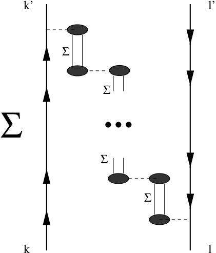
FIG. 2.: Effective Coulomb interactions with vacuum polarization being included. The geometrical sum of the vacuum polarization as an approximate complete set of “meson” states is taken. This figure is for $k^{\prime}>k$ and $l>l^{\prime}$. There is a similar (North-East) diagram for $k>k^{\prime}$ and $l^{\prime}>l$.

FIG. 3.: The deviation of the meson mass with the new bound state equation from that without vacuum polarization. Data are for $N=2000$ and for $N=3000$. The deviation is almost independent of $N$.

FIG. 4.: The limitation of the naive discretization. The results with the naive discretization are compared with those obtained by basis function calculation for the ’t Hooft-Bergknoff equation, the latter being considered to be accurate for small fermion masses. The naive discretization does not produce accurate values for small fermion masses.

FIG. 5.: The comparison of the wavefunctions obtained for the (“old”) ’t Hooft-Bergknoff equation and those for the “new” equation for $m=0.2$ and $m=1.0$. The wavefunctions for the new equation are less singular at the edges for small fermion masses.

TABLE I.: Comparison of the reduced calculation with the full one. The mass of the lowest meson state is shown. In the reduced calculation, we take only the first term in the sum in the screening factor (10). The calculations are done with the naive discretization explained in Sec. IV with $N=2000$.

fermion mass	reduced calculation	full calculation
0.1	1.07407458	1.07407437
0.5	1.84809454	1.84775659
1.0	2.82537904	1.84775659
5.0	1.06492610	1.06485924