[

A Density Matrix Renormalization Group Approach to
an Asymptotically Free Model with Bound States

Abstract

We apply the DMRG method to the 2 dimensional delta function potential which is a simple quantum mechanical model with asymptotic freedom and formation of bound states. The system block and the environment block of the DMRG contain the low energy and high energy degrees of freedom, respectively. The ground state energy and the lowest excited states are obtained with very high accuracy. We compare the DMRG method with the Similarity RG method and propose its generalization to field theoretical models in high energy physics.

]

A hallmark of an asymptotically free theory such as QCD is that it contains many degrees of freedom, with very different energy scales, which are coupled by the interaction Hamiltonian. Perturbative methods are valid for short distance physics but they fail for small momentum transfers or for energy scales where the bound states are formed. The existence of multiple energy scales suggests that the Renormalization Group approach is the correct strategy to attack these non perturbative problems. In recent years there has been several proposals to extract effective low energy Hamiltonians using RG methods. Of particular interest is the light-front Hamiltonian approach advocated in references [1, 2] which uses a similarity RG method (SRG) [3, 4]. In this method the RG flow is given by an unitary transformation which diagonalizes the Hamiltonian by succesive elimination of the off-diagonal matrix elements. The SRG-cutoff can be seen as the width of the band which contains the non vanishing off-diagonal matrix elements of the Hamiltonian. At the end of the SRG flow the width is zero and the corresponding Hamiltonian contains in its diagonal all the eigenvalues of the original one.

In this letter we shall propose an alternative RG approach to study asymptotically free models using the Density Matrix Renormalization Group (DMRG). We shall also show the relations and differences between the DMRG and the SRG methods. The DMRG was proposed by White in 1992 to solve the problems of the old real space RG methods encountered in the 70’s, which led in those days to their abandon in favour of Montecarlo techniques [5]. The DMRG has by now become a standard numerical RG method applied to many body problems in Condensed Matter and other branches of Physics ( see references [6, 7] for reviews). It is thus challenging to test how the DMRG handles the subtle dynamics of asymptotically free theories. To our knowledge this is the first paper devoted to the subject. For this reason we have choosen as a theoretical lab a simple model possesing the essential properties of asymptotic freedom and formation of bound states, which are shared by realistic theories like QCD.

The natural candidate for such a simple model is provided by a 2d quantum mechanical particle subject to a delta function potential [8]. The solution of the 2d delta function Schrödinger equation requires a regularization and renormalization schemes as in an ordinary quantum field theory. We shall use for our purposes the lattice regularization introduced by Glazek and Wilson in their SRG study of the problem [9, 10]. These authors formulated the problem in momentum space where the states are labelled by an integer $n$ that ranges between an infrared cutoff $M$ and an ultraviolet cutoff $N$ (i.e. $M\leq n\leq N$). The kinetic energy $E_{n}$ of the state $n$ increases exponentially as $E_{n}=b^{2n}$, where $b$ is an arbitrary constant greater than one. For numerical computations we shall take the value $b=\sqrt{2}$ as in references [9, 10]. The interaction Hamiltonian between the states $n$ and $m$ is given by $-g\sqrt{E_{n}E_{m}}$, where $g$ is the coupling constant of the problem. The discrete lattice Hamiltonian $H$ is defined by the matrix elements

$$H_{nm}=\delta_{n,m}b^{2n}-g\;b^{n+m},\;\;M\leq n,m\leq N$$ (1)

An overall shift of the levels by a constant term, i.e. $n\rightarrow n+n_{0}$, implies that $H_{nm}$ scales with the factor $b^{2n_{0}}$. This is a discrete version of scale invariance, which is broken by the infrared and ultraviolets cutoffs $M$ and $N$. The latter symmetry implies that all the scales contribute to the observables, which makes very hard an accurate determination of their value by methods other than the exact one.

The first step in the DMRG method is the partition of the system in two pieces called the system block and the environment block [5]. In our case we shall choose the system block $B^{L}_{\ell}$ to be given by the low energy levels $n$ which lie between the infrared cutoff $M$ and the scale $\ell$ (i.e. $M\leq n\leq\ell$), while the environment block $B^{H}_{\ell}$ will contain the high energy levels $n$ between the ultraviolet cutoff $N$ and the scale $\ell$ (i.e. $\ell\leq n\leq N$). The whole system, with energy levels ranging from $M$ to $N$, is obtained as the “superblock” $B^{L}_{\ell}\bullet\circ B^{H}_{\ell+3}$, where $\bullet$ and $\circ$ are the $n=\ell+1$ and $n=\ell+2$ energy levels respectively (see fig.1).

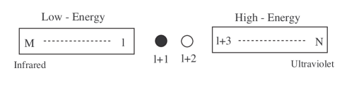
FIG. 1.: Superblock decomposition of the energy scales.

The parameter $\ell$ varies from $M$ to $N-3$ and it labels the DMRG flow. Let us supose we want to find the GS of the whole system. We shall choose a trial GS wave function $\psi_{\ell}(n)$ as follows,

$$\psi_{\ell}(n)=\left\{\begin{array}[]{lccl}a_{1}L_{\ell}(n)&&&M\leq n\leq\ell\\ a_{2}&&&n=\ell+1\\ a_{3}&&&n=\ell+2\\ a_{4}R_{\ell+3}(n)&&&\ell+3\leq n\leq N\end{array}\right.$$ (2)

where $L_{\ell}$ ( resp. $R_{\ell+3}$) is a normalized vector which describes the contribution of the low ( resp. high) energy block $B^{L}_{\ell}$ ( resp. $B^{H}_{\ell+3}$) to the GS of the superblock $B^{L}_{\ell}\bullet\circ B^{H}_{\ell+3}$. The ansatz (2) is the momentum space version of the real space DMRG applied by White to study a free particle in a box [6, 7]. Our approach is close in spirit to the momentum space DMRG method proposed by Xiang [11]. The energy of the state (2) can be conveniently written as

$$\langle\psi_{\ell}|H|\psi_{\ell}\rangle=\langle{\bf a}|H_{SB}(\ell)|{\bf a}\rangle$$ (3)

where $|{\bf a}\rangle$ is the vector $(a_{1},a_{2},a_{3},a_{4})$ and the superblock Hamiltonian $H_{SB}(\ell)$ is the $4\times 4$ matrix given by

$$H_{SB}(\ell)=\left(\begin{array}[]{cccc}h_{L}&h_{L\bullet}&h_{L\circ}&h_{LH}\\ h_{L\bullet}&h_{\bullet}&h_{\bullet\circ}&h_{H\bullet}\\ h_{L\circ}&h_{\bullet\circ}&h_{\circ}&h_{H\circ}\\ h_{LH}&h_{H\bullet}&h_{H\circ}&h_{H}\end{array}\right)$$ (4)

whose entries read

$$\begin{array}[]{ll}h_{L}=\langle L_{\ell}|H|L_{\ell}\rangle,&h_{H}=\langle R_{\ell+3}|H|R_{\ell+3}\rangle\\ h_{\bullet}=H_{\ell+1,\ell+1},&h_{\circ}=h_{\ell+2,\ell+2}\\ h_{L\bullet}=\sum_{n=M}^{\ell}H_{n,\ell+1}L_{\ell}(n),&h_{L\circ}=\sum_{n=M}^{\ell}H_{n,\ell+2}L_{\ell}(n)\\ h_{H\bullet}=\sum_{n=\ell+3}^{N}H_{n,\ell+1}R_{\ell+3}(n),&h_{LH}=\langle L_{\ell}|H|R_{\ell+3}\rangle\\ h_{H\circ}=\sum_{n=\ell+3}^{N}H_{n,\ell+2}R_{\ell+3}(n)&h_{\bullet\circ}=H_{\ell+2,\ell+3}\end{array}$$ (5)

where $H_{n,m}$ are the matrix elements given in eq. (1). Notice that eq.(3) takes the form of an eigenvalue problem in a reduced vector space with only 4 degrees of freedom. The GS of the superblock can be found by looking for the lowest eigenvalue $E_{1}(\ell)$ of the $4\times 4$ matrix $H_{SB}$. The variational nature of the construction gives an upper bound of the exact GS energy. If the vectors $L_{\ell}$ and $R_{\ell+3}$ coincide with the low energy and high energy pieces of the exact GS wave function then the DMRG algorithm presented so far would reproduce the exact result. Of course this is not in general the case but nevertheless, one can actually use the DMRG algorithm to improve in succesive steps the GS energy. The idea is to apply a continuity argument. Suppose we shift the scale $\ell$ to the next high energy level, say $\ell+1$. Then the new low energy vector $L^{\prime}_{\ell+1}$ will be related to the previous one $L_{\ell}$ by the equation

$$L^{\prime}_{\ell+1}(n)=\left\{\begin{array}[]{llll}a^{\prime}_{1}L_{\ell}(n)&&&M\leq n\leq\ell\\ a^{\prime}_{2}&&&n=\ell+1\end{array}\right.$$ (6)

where $(a^{\prime}_{1},a^{\prime}_{2})=(a_{1},a_{2})/\sqrt{a_{1}^{2}+a^{2}_{2}}$ is the normalized two component vector obtained by the projection of the lowest eigenvalue of $H_{SB}(\ell)$ into the block $B^{L}_{\ell}\bullet$. Similarly the energy $h^{\prime}_{L}(\ell+1)$ associated to the latter block is given by

$$h^{\prime}_{L}(\ell+1)=(a^{\prime}_{1},a^{\prime}_{2})\left(\begin{array}[]{ll}h_{L}(\ell)&h_{L\bullet}(\ell)\\ h_{L\bullet}(\ell)&h_{\bullet}(\ell)\end{array}\right)\left(\begin{array}[]{c}a^{\prime}_{1}\\ a^{\prime}_{2}\end{array}\right)$$ (7)

The data $L^{\prime}_{\ell+1}$ and $h^{\prime}_{L}(\ell+1)$ fully characterize the new block $B^{\prime L}_{\ell+1}$ which can be regarded as the renormalization of the block $B^{L}_{\ell}\bullet$. The next step is to construct the superblock $B^{L}_{\ell+1}\bullet\circ B^{H}_{\ell+4}$ which by the same techniques leads to the construction of a new block $B^{\prime L}_{\ell+2}$ and so on. This procedure is iterated until the scale $\ell=N-3$, where one reverses the DMRG steps in order to update the high energy blocks $B^{H}_{\ell}$ using the low energy blocks built in the previous steps. After a few sweeps from low to high energy and viceversa the lowest eigenvalue of the superblock Hamiltonian (4) converges to a fix value which gives the DMRG estimation of the GS energy. To start out the process one has to grow up the system to its actual size. This can be done by considering superblocks of the form $B^{L}_{M+p}\bullet\circ B^{H}_{N-p}$ where $p=0,\dots,(N-M-3)/2$. The last value of $p$ yields a system containing all the scales from $M$ to $N$. The low and high energy blocks constructed in the warm up are the starting point for the sweeping procedure explained above (see [6, 7] for details). The previous algorithm has been generalized in reference [12] to find out not only the GS but the low lying excitations as well.

Let us now present our DMRG results for the case considered in references [9, 10], where $M=-21,N=16$ and $g=0.06060600032108866$. The latter value of $g$ is choosen in such a way that the exact ground state energy of (1) is given exactly by $-1$. The DMRG algorithm presented above gives the exact ground state energy with an error of $10^{-14}$ (see table 1). Using the extension of the DMRG proposed in [12] we have also computed the GS and the lowest 3 excited states of the Hamiltonian (1). In table 1 we compare our DMRG results with the exact ones in terms of the relative deviation

$$\delta E_{n}=\frac{E_{n}(DMRG)-E_{n}(exact)}{E_{n}(exact)}$$ (8)

Table 1. Relative error $\delta E_{n}$ of the four lowest eigenstates of the Hamiltonian (1).

As shown in table 1 the accuracy of the excited states energies is lower than that of the GS. This feature is peculiar to the delta function Hamiltonian and it does not arise for the quantum mechanical models studied in [12]. There are several reasons for the very high accuracy of the DMRG applied to the Hamiltonian (1): i) the DMRG gives a variational upper bound to the exact GS energy which is usually improved in every DMRG step; ii) all the matrix elements of the whole Hamiltonian are used many times to feedback the superblock so that no information is lost; iii) the DMRG method focus on the determination of the GS and the low lying states.

In fig.2 we plot the DMRG wave function which after the third sweep is indistinguishable from the exact one.

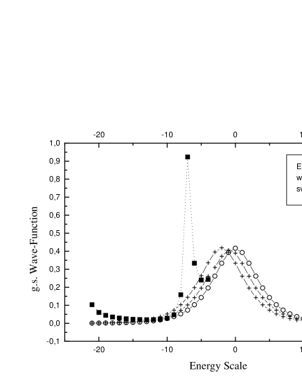
FIG. 2.: DMRG v.s. exact wave function.

It is interesting to investigate the nature of the DMRG flow as compared with the one of the similarity RG method. In the SRG the effective Hamiltonian $H(s)$ evolves as a function of $s$ according to the Wegner equation [4],

$$\frac{dH(s)}{ds}=[[H_{d}(s),H(s)],H(s)]$$ (9)

where $H_{d}(s)$ is the diagonal part of $H(s)$. The initial condition of eq.(9) is $H(0)=H$, where $H$ is the original Hamiltonian of the problem. The parameter $s$ ranges from $0$ to $\infty$ and it can be identified with the inverse square of the energy width $\lambda$, i.e. $s=1/\lambda^{2}$. Eq. (9) implies that $H(s)$ is related to $H$ by an unitary transformation and therefore they share their eigenvalues. When $s$ increases, the off diagonal matrix elements of $H(s)$, located at distances greater than the width $\lambda=1/\sqrt{s}$, become very small. When $s=\infty$ the effective Hamiltonian $H(\infty)$ is diagonal and all its entries coincide with the eigenvalues of $H$. The numerical integration of eq.(9) requires of course to follow the evolution of all the entries of $H$. One would like instead to project the effective Hamiltonians to smaller (“window”) matrices in order to reproduce the bound state eigenvalue [10]. In a sense, the superblock $4\times 4$ matrices (4) resemble the window matrices of ref. [10]. Motivated by the SRG ideas [10], we have studied the RG flow of the eigenvalues $E_{i}(\ell)(i=1,\dots,4)$ of the superblock Hamiltonian (4). In fig.3 we plot the lowest eigenvalue $E_{1}$, together with the remaining ones scaled down by a factor $b^{2\ell}$. We can clearly see from fig.3 that $E_{1}$ stays constant through all the DMRG steps while $E_{i}(i=2,3,4)$ vary with the energy scale $b^{2\ell}$ with some deviations depending on the energy region. The plateaus correspond to low energy regions while the oscillations and bumps occur for intermediate and high energies. To a first order approximation, which is almost exact for the plateaus, the superblock Hamiltonian (4) can be written as

$$H_{SB}(\ell)=O_{\ell}\left(\begin{array}[]{cccc}E_{1}&0&0&0\\ 0&E^{\prime}_{2}b^{2\ell}&0&0\\ 0&0&E^{\prime}_{3}b^{2\ell}&0\\ 0&0&0&E^{\prime}_{4}b^{2\ell}\end{array}\right)O^{\dagger}_{\ell}$$ (10)

where $O_{\ell}$ is a unitary matrix. Using eq.(10) one can show that the superblock Hamiltonians satisfy the following second order recursion relation,

$$H_{SB}(\ell)=$$ (11)

$$\frac{1}{b+b^{-1}}\left(b^{-1}U_{\ell}H_{SB}(\ell+1)U^{\dagger}_{\ell}+bU^{\dagger}_{\ell-1}H_{SB}(\ell-1)U_{\ell-1}\right)$$ (12)

where $U_{\ell}=O_{\ell}O^{\dagger}_{\ell+1}$. The continuum limit of eq.(11) gives the flow equations

$$H_{1}\equiv\frac{dH_{SB}}{d\ell}-[\eta,H_{SB}],\;\;\frac{dH_{1}}{d\ell}=[\eta,H_{1}]$$ (13)

where $\eta=\frac{dO_{\ell}}{d\ell}O^{\dagger}_{\ell}$. Eq.(14) is a second order diferential equation which is to be compared with the first order equation eq.(9). The DMRG flow is a sort of similarity transformation with some eigenvalues running with the scale. Using the standard RG terminology the lowest eigenvalue $E_{1}$ can be associated with a marginal operator while the eigenvalues $E_{i}$ for $i=2,3,4$ are associated with infrared irrelevant operators which vanish at the fixed point Hamiltonian $H_{SB}(\ell=M)$. Indeed all the entries of $H_{SB}(\ell=M)$ are very small except for the entry $h_{H}=-0.999$ whose value is close to the bound state energy. These results suggest that the exactness of the DMRG method is due to a careful treatment of the irrelevants operators, which in other RG methods are difficult to control in general.

From a conceptual point of view the DMRG offers a new way of thinking about cutoffs and RG flows in high energy physics. Traditional cutoffs remove high energy states while the lowering of the cutoff produces effective operators for lower energies [13]. In the Lagrangian formulation this strategy can be implemented perturbatively without much difficulty. However in the Hamiltonian formulation it gives rise to small denominators problems involving energy differences between the states kept and the states truncated in the RG process [14, 9]. This latter problems do not arise in the DMRG truncation for it uses a non perturbative self-consistent algorithm to find the best choice of the effective Hilbert spaces and Hamiltonians.

The next step in the application of the DMRG to high energy physics is of course to consider field theoretical models with asymptotic freedom and bound states.

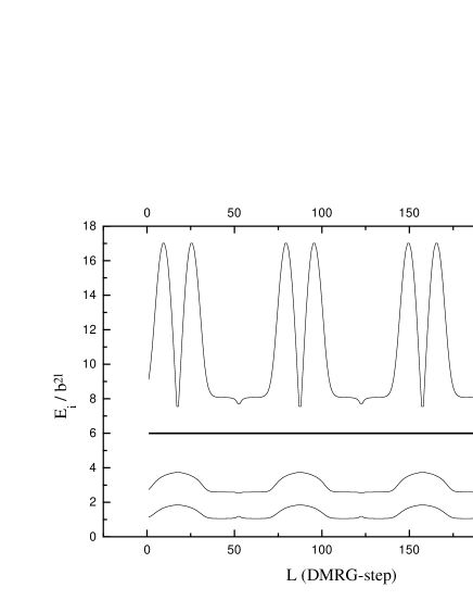
FIG. 3.: Plot of the rescaled superblock eigenvalues $E_{i}/b^{2\ell}$ ($i=2,3,4$) as a function of the DMRG step L from sweep 2 to 4.

The most appropriate formalism for this application of the DMRG is known as Discrete Light-Cone Quantization in momentum space (DLCQ) [15], [16]. In the DLCQ approach the Hilbert space is finite dimensional and the light-front Hamiltonian $H_{LC}$ acting on it is similar to that of a many-body Hamiltonian in condensed matter [16]. The search for bound states amounts to solving the Schroedinger equation

$$H_{LC}|\psi\rangle=M^{2}\;|\psi\rangle$$ (14)

where $M^{2}$ is the mass of the bound state. Thus, one can apply to (14) standard diagonalization techniques such as Lanczos. The DMRG method allows us to study larger Hilbert spaces than those achieved with the Lanczos method. This is needed in order to recover the continuum limit of $H_{LC}$.

The key to make the clever truncation of states in the RG process is given by the density matrix of the blocks. This is a systematic procedure with no wild guessing about the wave function. A given block will contain the most representative multiparticle and momentum states in order to reconstruct the lowest lying bound states. On the other hand, the DMRG is a numerical method, unlike the more analytical SRG method [17], and does not need perturbative inputs. The basic requirement for the DMRG method to work is a discretized Hamiltonian acting on finite dimensional Hilbert spaces. As a first test of this program we have solved eq.(14) for the Positronium state of the massive and massless Schwinger model in the one-fermion sector with the DMRG. These results will be reported elsewhere.

Thefore, we expect that the main ideas presented in this letter can be generalized to the DLCQ Hamiltonians. Specifically, the breaking of the system into low energy and high energy blocks which are constantly updated through the DMRG process. On the other hand the DMRG method combined with the DLCQ approach does not have the sign problems that emerge in the Montecarlo methods used in Lattice Gauge Theories [16]. In summary, we believe that the power shown in condensed matter systems by the DMRG method is worthwhile to be translated into Particle Physics.

Acknowledgements This work was supported by the DGES spanish grant PB97-1190.

REFERENCES

- [1] K.G. Wilson et al. , Phys. Rev. D 49, 6720 (1994).
- [2] R.J. Perry, nucl-th/9901080.
- [3] St. D. Glazek and K.G. Wilson, Phys. Rev. D 48, 5863 (1993); 49, 4214 (1994).
- [4] F. Wegner, Ann. Physik 3, 77 (1994).
- [5] S.R. White, Phys. Rev. Lett. 69, 2863 (1992), Phys. Rev. B 48, 10345 (1993).
- [6] S.R. White, Phys. Rep. 301, 187, (1998).
- [7] R. Noack and S.R. White, Lecture Notes in Physics, I.Peschel, X. Wand, K. Hallberg, eds. (Springer-Verlag, 1999).
- [8] R. Jackiw, in M.A.B. Beg Memorial Volume, A. Ali and P. Hoddbhoy, eds. (World Scientific, Singapore, 1991).
- [9] K.G. Wilson and St. D. Glazek, in the Procs. of the Ninth Physics Summer School at the Australian National University, H.J. Gradner and C.M. Savage, eds. (World Scientific, Singapore, 1997).
- [10] St. D. Glazek and K.G. Wilson, hep-th/9707028.
- [11] T. Xiang, Phys. Rev. B 56, 5061 (1996).
- [12] M.A. Martín-Delgado, G. Sierra and R. Noack, cond-mat/9903100.
- [13] K. G. Wilson, Phys. Rev. 140, B445 (1965).
- [14] C. Bloch and J. Horowitz, Nucl. Phys. 8, 91 (1958).
- [15] H.-C. Pauli and S. J. Brodsky, Phys. Rev. D 32, 1993, 2001 (1985).
- [16] T. Eller, H.-C.Pauli, and S. J. Brodsky, Phys. Rev. D 35, 1493 (1987). For a review, see S. Brodsky, H-C Pauli, S. Pinsky, Phys.Rept. 301 (1998) 299-486.
- [17] St. D. Glazek, Acta Phys. Pol. B29 (1998) 1979-2064, hep-th/9712188.