Renormalizability and the scalar field

Abstract

The infinite dimensional generalization of the quantum mechanics of extended objects, namely, the quantum field theory of extended objects is presented. The paradigm example studied in this paper is the Euclidean scalar field with a $\lambda{\phi^{6}}/{6!}$ interaction in four spacetime dimensions. The theory is found to be finite when the virtual particle intermediate states are characterized by fuzzy particles instead of ordinary pointlike particles. Causality, Lorentz invariance, and unitarity (verified up to fourth order in the coupling constant) are preserved in the theory. In addition, the Kallen-Lehmann spectral representation for the propagator is discussed.

I Introduction

The necessity to incorporate the finite extent or fuzziness of a quantum particle into our description of the world and the resulting quantum mechanics have been presented by the author[1]. In the extended object formulation we have noncanonical commutation relations of the form

$$\left[X_{f_{i}},P_{j}\right]=ie^{-P^{2}/m^{2}}\delta_{ij},\mbox{ and }\left[X_{f_{0}},P_{0}\right]=-ie^{-P_{0}^{2}/m^{2}},$$ (1)

where $X_{f}$ is the noncommuting position operator and $P^{2}=P_{i}P^{i}$. In terms of Euclidean momenta we can write the commutation relations as

$$\left[X_{f_{\mu}},P_{\nu}\right]=ie^{-P^{2}/m^{2}}g_{\mu\nu},$$ (2)

where $P_{\nu}$ is the Euclidean 4-momentum, and $g_{\mu\nu}=(1,1,1,1)$ is the Euclidean metric and $P^{2}$ is a Euclidean scalar. The commutation relations in Eq. (2) have a smooth limit with ordinary quantum mechanics as the Compton wavelength ${1}/{m}$ of the particle vanishes. Our goal is to understand the infinite dimensional generalization of the quantum mechanics based on these commutation relations, namely, the quantum field theory of extended objects. The characterization of intermediate states by fuzzy particles obeying the commutation relations in Eq. (2) becomes important in rendering finite, hitherto nonrenormalizable theories because the troublesome vertex which causes these divergences is effectively smeared out. In this paper we restrict ourselves to the simple case of the Euclidean scalar field with a $\lambda{\phi^{6}}/{6!}$ interaction which has been found to be nonrenormalizable when approached via the quantum field theory of point particles. We choose to construct the field theory in Euclidean space for convenience. The generalization of the commutation relations in Eq. (2) to continuous systems (fields) and the subsequent development of the theory leads to a Euclidean momentum space propagator which can render the interacting field theory finite to all orders. The theory is found to obey causality and Lorentz invariance, and unitarity is demonstrated up to fourth order in the coupling constant. In addition, the Kallen-Lehmann spectral representation for the propagator is presented. We note that Lorentz invariance of such quantities as propagation amplitudes and scattering amplitudes is ensured when we employ a Euclidean formulation by virtue of the variable transformation $p_{0}\rightarrow ip_{0}$. This cannot be viewed as a rotation of the contour in the sense of the Wick rotation (since the contour does not close), and as we shall demonstrate such a transformation recovers the Minkowski space propagation amplitude. Thus, preservation of the four dimensional rotational symmetry of Euclidean space will also preserve Lorentz invariance.

II The Scalar Field

Super-renormalizable and renormalizable quantum field theories are characterized by the dimensionality of their coupling constants which have positive mass dimension or are dimensionless. In the first case, the perturbation expansion of the N-point functions or scattering amplitudes have positive length dimension and the degree of divergence of the graphs becomes smaller as more vertices are included. In renormalizable theories, the perturbation expansions are dimensionless and only a finite number of amplitudes superficially diverge; however, divergences occur at all orders in perturbation theory and can be automatically removed by a redefinition of a finite number of physical constants. Nonrenormalizable theories are characterized by negative dimensional coupling constants. Consequently, the perturbation expansions have dimension $\frac{1}{length}$ and as we include more vertices the degree of divergence becomes larger.

A point particle renormalizable theory can be rendered finite by implementing regularization procedures; for example, by introducing a high momentum cut off $\Lambda$ in which case we renounce all interest in regions less than $\Lambda^{-1}$ and consequently, the point of interaction (the vertex) is fuzzed out. However, such procedures fail to render nonrenormalizable theories finite while preserving essential features such as gauge invariance, Lorentz invariance, and unitarity. Instead of introducing such cut offs we can take advantage of the fuzziness inherent in the particle to place an effective lower bound on the short distances. It is for this reason that we introduce fuzzy particle intermediate states in a nonrenormalizable theory.

The Euclidean space Lagrangian for the scalar field with a $\lambda\phi^{6}/6!$ interaction is written as

$${\cal L}=\frac{1}{2}(\partial_{\mu}\phi)^{2}+\frac{1}{2}m^{2}\phi^{2}+\lambda\frac{\phi^{6}}{6!},$$ (3)

where $\lambda$ is a negative dimensional coupling constant. The free scalar field is usually approached by expanding the field as a sum over 3-momenta of independent harmonic oscillators. The starting point for such a treatment is the Klein-Gordon equation and the promotion of classical fields to operators is achieved by the imposition of canonical commutation relations. If we compute the propagation amplitude from the field expansion we recover the Green’s function of the Klein-Gordon operator. This is expected since the canonical commutation relations are quantum mechanical generalizations of the Poisson brackets found in classical mechanics. Furthermore, since a point particle can be localized with arbitrary precision, we are able to characterize such particles as existing in well defined 3-momentum states at any instant in time. When we generalize the extended object formulation of quantum mechanics we are unable to retain this characterization because the particle is smeared out in a small region of spacetime. In order to incorporate the smearing in the time direction into our infinite dimensional generalization, we have to characterize a fuzzy particle by its 4-momentum or its mass (when on shell). Moreover, the commutation relations that arise in the extended object formulation cannot be viewed as simple quantum mechanical generalizations of the classical Poisson brackets since the Compton wavelength of classical particles vanishes. It is to be noted that any attempt to impose the noncanonical commutation relations in the usual approach will violate Lorentz invariance since the commutator between the field and the momentum density as a function of 3-momentum:

$$\left[\phi({\bf p}),\pi({\bf q})\right]=ie^{-p^{2}/m^{2}}\delta^{(3)}({\bf p}-{\bf q}),$$ (4)

where $p^{2}={\bf p}^{2}$ will not be a Lorentz invariant quantity and which in turn leads to acausal behavior in the theory. The reason for this behavior is because such a generalization introduces fuzziness in space but not in the time direction: for example, consider the instantaneous annihilation of a particle of finite extent. As a consequence, we adopt a unified, Lorentz invariant, spacetime generalization of the extended object formulation to fields given by

$$\left[\phi(p),\pi(q)\right]=ie^{-p^{2}/m^{2}}\delta^{(4)}(p-q),$$ (5)

where $p^{2}=p_{\mu}p^{\mu}$ is a Euclidean scalar. This generalization allows us to characterize the fuzzy particle intermediate states as well defined 4-momentum states or as a collection of masses (when on shell). We are now in a position to write down the field expansion for $\phi(x)$,

$$\phi(x)=\int\frac{d^{4}p}{(2\pi)^{4}}\frac{1}{\sqrt{p^{2}+m^{2}}}(a_{p}e^{-ipx}+a^{\dagger}_{p}e^{ipx}),$$ (6)

and the corresponding momentum density,

$$\pi(x)=\int\frac{d^{4}p}{(2\pi)^{4}}(-i)\sqrt{p^{2}+m^{2}}(a_{p}e^{-ipx}-a^{\dagger}_{p}e^{ipx}).$$ (7)

The weights in the above equations have been chosen so that, with canonical commutations underlying, $\left[a_{p},a^{\dagger}_{q}\right]=(2\pi)^{4}\delta^{(4)}(p-q)$, we obtain

$$D_{R}(x-y)=\langle 0|\phi(x)\phi(y)|0\rangle=\int\frac{d^{4}p}{(2\pi)^{4}}\frac{1}{p^{2}+m^{2}}e^{-ip(x-y)},$$ (8)

which is the retarded scalar field propagator or the Green’s function for the Klein-Gordon operator. We observe that Eq. (8) is symmetric under $x\leftrightarrow y$ (just change $p\rightarrow-p$) implying that $\left[\phi(x),\phi(y)\right]=0$ for all $x$ and $y$.The vanishing of this commutator can be explained by noting that $\phi(x)$ is a field which creates and destroys 4-momentum (or mass) states and the measurement of such a field at one spacetime point cannot affect the measurement at another spacetime point since 4-momentum states are relativistic invariants. However, there is a nonzero propagation amplitude for 4-momentum states. Let us denote by $\phi^{(3)}(x)$ the usual 3-momentum expansion of the field obtained by quantizing the classical equation of motion, that is,

$$\phi^{(3)}(x)=\int\frac{d^{3}p}{(2\pi)^{3}}\frac{1}{\sqrt{2E_{{\bf p}}}}(a_{p}e^{-ipx}+a^{\dagger}_{p}e^{ipx}),$$ (9)

where $E_{{\bf p}}=\sqrt{{\bf p}^{2}+m^{2}}$. Then from Eq. (8) it follows that

$$D_{R}(x-y)=\langle 0|\phi(x)\phi(y)|0\rangle=\theta(x^{0}-y^{0})\langle 0|[\phi^{(3)}(x),\phi^{(3)}(y)]|0\rangle.$$ (10)

Thus, the 4-momentum expansion generates the correct propagation amplitude for the scalar field which admits a representation as the vacuum expectation value of the commutator of 3-momentum field expansions. Since the ordinary scalar field is quantized by generalizing the spatial commutation relations obtained from ordinary quantum mechanics to infinite dimensions, time remains a parameter, and questions of causality arise. It is well known that this commutator vanishes over spacelike intervals and that causality is preserved in the ordinary scalar field. This is expected since the propagation amplitude for the ordinary scalar field can also be obtained from a Lorentz invariant, spacetime generalization of a causal structure, namely, ordinary quantum mechanics. When we impose noncanonical commutation relations $\left[a_{p},a^{\dagger}_{q}\right]=(2\pi)^{4}e^{-p^{2}/m^{2}}\delta^{(4)}(p-q)$ on the field and momentum density expansions we obtain the propagation amplitude describing intermediate states as:

$$D(x-y)=\langle 0|\phi(x)\phi(y)|0\rangle=\int\frac{d^{4}p}{(2\pi)^{4}}\frac{e^{-p^{2}/m^{2}}}{p^{2}+m^{2}}e^{-ip(x-y)}.$$ (11)

We once again observe the symmetry under $x\leftrightarrow y$ (by changing $p\rightarrow-p$) which reflects the fact that $\phi(x)$ creates and destroys relativistically invariant 4-momentum states. The correspondence between Euclidean space and Minkowski space propagation amplitudes is effected by means of the variable transformation $p_{0}\rightarrow ip_{0}$ which has been mentioned before. This cannot be viewed as a rotation of the contour in the sense of the Wick rotation since the contour of integration does not close in this case. We note that the corresponding $dp_{0}$ integration limits in Minkowski space go from $-i\infty$ to $i\infty$. In order to explain this feature, consider the commutation relations arising from the quantum mechanics of extended objects

$$\left[X_{f_{i}},P_{j}\right]=ie^{-P^{2}/m^{2}}\delta_{ij},\mbox{ and }\left[X_{f_{0}},P_{0}\right]=-ie^{-P_{0}^{2}/m^{2}},$$ (12)

where $P^{2}=P_{i}P^{i}$. The spacetime generalization of these commutation relations in Minkowski space can be achieved by writing them as

$$\left[X_{f_{\mu}},P_{\nu}\right]=i\eta_{\mu\nu}e^{-P^{2}/m^{2}},$$ (13)

where $P^{2}=P_{\mu}P^{\mu}$ is a Lorentz scalar and $\eta_{\mu\nu}=(-1,1,1,1)$. However, such spacetime commutation relations do not lend themselves to a Lorentz invariant generalization to fields due to the presence of the Minkowski metric. The only other possibility is to re-express the fuzzy time and energy commutation relation as

$$\left[iX_{f_{0}},iP_{0}\right]=ie^{-P_{0}^{2}/m^{2}}$$ (14)

in order to get rid of the relative negative sign in Eq. (12). This would imply that the $dp_{0}$ integration limits would now go from $-i\infty$ to $i\infty$ and it is for this reason that the Minkowski space propagation amplitude remains bounded in spite of the positive term in the exponential. If the contour of integration were to close this would be a Wick rotation as is the case in the limit of vanishing Compton wavelength. Equivalently, we can formulate the theory in Euclidean space. The Euclidean momentum space propagator is given by:

$${\tilde{D}(p)}=\frac{e^{-p^{2}/m^{2}}}{p^{2}+m^{2}},$$ (15)

which is bounded from above and below since $p^{2}$ is a Euclidean scalar. In the limit as the Compton wavelength vanishes we recover the usual scalar field propagator (Euclidean). We note that in arriving at this propagator we have employed a different quantization prescription but we have not changed the Lagrangian, that is, the classical field theory is left undisturbed. Since the quantization prescription arises from the quantum mechanics of extended objects which has no classical counterpart, we are justified in employing this procedure. A crucial feature of this propagator is the Gaussian damping which renders the theory finite; for example, insertion of an arbitrary number of vertices in the N-point function of a $\phi^{6}$ theory would no longer make the graphs divergent because the Gaussian damping eliminates the high frequency modes. Since the extended object formulation is a causal structure its infinite dimensional, Lorentz invariant, generalization will obey causality. In order to prove that causality is not violated we need to establish that the propagation amplitude for 4-momentum states given in Eq. (11) does not admit a representation as the vacuum expectation value of the commutator of two 3-momentum field expansions. This is crucial since the propagation amplitude does not vanish over spacelike intervals but this in itself does not violate causality. The correct statement of causality requires us to determine whether a measurement made at one spacetime point can affect a measurement made at another spacetime point outside the light cone. Causality is preserved if the commutator of two 3-momentum field expansions vanishes over spacelike intervals provided $\phi^{(3)}(x)$ exists. If $\phi^{(3)}(x)$ does not exist the nonvanishing of the propagation amplitude over spacelike intervals will have no implication for causality. In scalar field theory with canonical commutation relations underlying we are able to construct field expansions $\phi^{(3)}(x)$ for intermediate states which are sum over 3-momenta of independent harmonic oscillators obtained by simply quantizing the Klein-Gordon equation. We observe that with noncanonical commutation relations underlying we can no longer construct $\phi^{(3)}(x)$ because well defined 3-momentum characterizations for fuzzy particle states do not exist which we expect from considerations of Lorentz invariance and causality. In order to prove that it is impossible to construct well defined 3-momentum states for fuzzy particles, assume that there exists $\phi^{(3)}(x)$ such that

$$\theta(x^{0}-y^{0})\langle 0|[\phi^{(3)}(x),\phi^{(3)}(y)]|0\rangle=\int\frac{d^{4}p}{(2\pi)^{4}}\frac{e^{-p^{2}/m^{2}}}{p^{2}+m^{2}}e^{-ip(x-y)}.$$ (16)

In particular, for $x=y$, we require that

$$\int{d^{4}p}\frac{e^{-p^{2}/m^{2}}}{p^{2}+m^{2}}=0.$$ (17)

The Euclidean momentum space integral can be easily evaluated by employing the variable transformation $p^{2}=u$ but in order to demonstrate a method which will be useful in proving unitarity, we adopt a different approach. Due to the essential singularity at infinity the $dp_{0}$ integral cannot be evaluated by contour integration. Switching to dimensionless variables we wish to evaluate

$$\int_{-\infty}^{\infty}dx\frac{e^{-x^{2}}}{x^{2}+x_{0}^{2}}=\frac{1}{2ix_{0}}\left[\int_{-\infty}^{\infty}dx\frac{e^{-x^{2}}}{x-ix_{0}+i\epsilon}-\int_{-\infty}^{\infty}dx\frac{e^{-x^{2}}}{x+ix_{0}+i\epsilon}\right].$$ (18)

So the problem is reduced to finding

$$f(x_{0})=\int_{-\infty}^{\infty}dx\frac{e^{-x^{2}}}{x-ix_{0}+i\epsilon},$$ (19)

which defines the so called Hilbert transform. Now

$$\frac{df(x_{0})}{dx_{0}} = \int_{-\infty}^{\infty}dxe^{-x^{2}}\frac{d}{dx_{0}}\frac{1}{x-ix_{0}+i\epsilon}$$ (20)

$$= -i\int_{-\infty}^{\infty}dxe^{-x^{2}}\frac{d}{dx}\frac{1}{x-ix_{0}+i\epsilon}$$ (21)

$$= i\int_{-\infty}^{\infty}dx\frac{1}{x-ix_{0}+i\epsilon}\frac{d}{dx}e^{-x^{2}}$$ (22)

$$= -i\int_{-\infty}^{\infty}dxe^{-x^{2}}\frac{2x}{x-ix_{0}+i\epsilon}$$ (23)

$$= -2i\int_{-\infty}^{\infty}dxe^{-x^{2}}\left[1+\frac{ix_{0}}{x-ix_{0}+i\epsilon}\right]$$ (24)

$$= -2i\sqrt{\pi}+2x_{0}f(x_{0}).$$ (25)

If we multiply this differential equation by $e^{-x_{0}^{2}}$ and integrate from $0$ to $x_{0}$ using the initial value $f(0)=i\pi$ obtained by simple contour integration we get

$$e^{-x_{0}^{2}}f(x_{0})=i\pi-2i\sqrt{\pi}\int_{0}^{x_{0}}dx^{\prime}e^{-x^{\prime 2}}.$$ (26)

If we define $erf(x_{0})=\frac{2}{\sqrt{\pi}}\int_{0}^{x_{0}}dye^{-y^{2}}$ we can express the solution as

$$f(x_{0})=i\pi e^{x_{0}^{2}}[1-erf(x_{0})].$$ (27)

Using this formula we can evaluate the 4-momentum integral to obtain

$$\int d^{4}p\frac{e^{-p^{2}/m^{2}}}{p^{2}+m^{2}}=\frac{-2\pi e}{m^{2}}\int\frac{d^{3}p}{2E_{{\bf p}}}erf(E_{{\bf p}}),$$ (28)

where $E_{\bf p}=\sqrt{{\bf p}^{2}+m^{2}}$. The 3-momentum integral over the error function is a nonzero quadrature and we arrive at a contradiction to our original requirement that the integral in Eq. (17) vanish. As the Compton wavelength vanishes ($\frac{1}{m}\rightarrow 0$) the left hand side of Eq. (28) reverts to the ordinary scalar field propagator (for $x=y$) and the right hand side vanishes, a result we expect. Hence, the existence of 3-momentum characterizations for fuzzy particle states would have been an indication of acausal behavior. Similarly, we can demonstrate that there exists no $\phi^{(3)}(x)$ which can satisfy Eq. (16) for $x\neq y$. Evaluation of the propagation amplitude for $x\neq y$ leads to a sum of error functions of arguments involving $x-y$ and a functional form for $\phi^{(3)}(x)$ as a sum of creation and annihilation operators becomes impossible to obtain. Thus, the fact that we have constructed the field theory from a Lorentz invariant, spacetime generalization of a causal formulation, namely, the quantum mechanics of extended objects, combined with the fact that 3-momentum characterizations do not exist for fuzzy particle intermediate states allows us to conclude that the statement of causality is not violated in the theory.

III unitarity in the theory

The optical theorem relates the forward scattering amplitude to the total cross section for production of all final states. Since the imaginary part of the forward scattering amplitude gives the attenuation of the forward going wave as the beam passes through the target, it is natural that this quantity should be proportional to the probability of scattering[2]. In the quantum field theory of point particles each diagram contributing to an S-matrix element is purely real unless some denominators vanish so that the $i\epsilon$ prescription for treating the poles becomes relevant, that is, a Feynman diagram yields an imaginary part for the scattering amplitude ${\cal M}$ only when the virtual particles in the diagram go on mass shell. In the quantum field theory of extended objects because of the Gaussian damping term in the propagator the scattering amplitude exhibits an imaginary part even below the threshold for production of multiparticle states. However, this is the unphysical part of the scattering amplitude and does not contribute to the optical theorem since we only need to verify whether the physical scattering amplitude which lies above the threshold for the production of multiparticle states is equal to the total cross section for the production of all such states. Let us first calculate the scattering amplitude at order-$\lambda^{2}$ with a $\phi^{6}$ interaction. The order-$\lambda^{2}$ diagram is shown in figure 1 and the contribution of this diagram is given by the Lorentz invariant integral

$$i\delta{\cal M}=\frac{\lambda^{2}}{2}\int\frac{d^{4}q}{(2\pi)^{4}}\frac{e^{-(\frac{k}{2}+q)^{2}/m^{2}}}{(\frac{k}{2}+q)^{2}+m^{2}}\frac{e^{-(\frac{k}{2}-q)^{2}/m^{2}}}{(\frac{k}{2}-q)^{2}+m^{2}},$$ (29)

where $k=\sum_{i=1}^{4}k_{i}$ and we have chosen a symmetric routing of momenta. We observe that the because of the dimensional coupling (mass dimension = -2) we would need to increase the powers of momentum in the integrand in order to render the graph dimensionless, but because of the Gaussian damping factors the graphs will not diverge at any order. Due to the essential singularities in the integrand arising due to the Gaussian damping terms in the propagators, this integral cannot be evaluated by contour integration and for the same reason the Cutkosky cutting rules do not apply. Consequently, we employ the standard method of Feynman parameters to obtain

$$i\delta{\cal M}=\frac{\lambda^{2}}{16\pi^{2}}\int_{0}^{1}dxe^{-k^{2}/2m^{2}}\int_{0}^{\infty}dl\,l^{3}\frac{e^{-2l^{2}/m^{2}-2lk/m^{2}}}{(l^{2}+\Delta)^{2}},$$ (30)

where $l=q+\frac{kx}{2}-\frac{k(1-x)}{2}$ and $\Delta=k^{2}x(1-x)+m^{2}$. We note that since we are dealing with Euclidean momenta, a Wick rotation would be superfluous. The imaginary part shows up in the $dl$ integration which can be recast as

$$\left.\frac{d}{d\Delta}\frac{d^{3}}{d\alpha^{3}}e^{-\frac{k^{2}}{2m^{2}}(1-\alpha^{2})}\int_{0}^{\infty}dl\frac{e^{-\frac{2}{m^{2}}(l+\frac{\alpha k}{2})^{2}}}{(l^{2}+\Delta)}\right|_{\alpha=1}.$$ (31)

The integral can be evaluated by the formula developed in the previous section and noting that Eq. (31) contains a shifted Gaussian and that the integration limits are from $0$ to $\infty$ we obtain

$$i\delta{\cal M}=\frac{\lambda^{2}}{16\pi^{2}}(\frac{m^{2}}{2k})^{3}\int_{0}^{1}dx\frac{d}{d\Delta}\frac{d^{3}}{d\alpha^{3}}e^{-\frac{k^{2}}{2m^{2}}(1-\alpha^{2})}\times$$ (33)

$$\left.\left[\frac{1}{2i\sqrt{\Delta}}\left(h(k)-i\frac{\pi}{2}erfc(\frac{\alpha k}{m\sqrt{2}})erf(\frac{i\alpha k}{m\sqrt{2}}-\sqrt{\Delta})\right)e^{({i\alpha k}/{m\sqrt{2}}-\sqrt{\Delta})^{2}}+(\sqrt{\Delta}\,\leftrightarrow\,-\sqrt{\Delta})\right]\right|_{\alpha=1},$$

where

$$h(k)=\left(\int_{\frac{\alpha k}{m\sqrt{2}}}^{\infty}\!\!+\>e^{-\alpha^{2}k^{2}/2m^{2}}\!\int_{\frac{i\alpha k}{m\sqrt{2}}}^{\sqrt{\Delta}}\right)dx\frac{e^{-x^{2}}}{x},$$ (34)

and $erfc$ is the complementary error function. Consider the analytic structure of the scattering amplitude. The square root of $\Delta$ has a branch cut when its argument becomes negative, that is, when

$$k^{2}x(1-x)+m^{2}<0.$$ (35)

The product $x(1-x)$ is at most $\frac{1}{4}$ so ${\cal M}(k)$ has a branch cut beginning at

$$k^{2}=-4m^{2}$$ (36)

at the threshold for the creation of a multiparticle state. When $\Delta<0$ (that is, $-k^{2}>4m^{2}$) $h(k)$, and the exponential factors in Eq. (33) become purely real, and since

$$erf(ix)=\frac{i}{\sqrt{2\pi}}\int_{0}^{x}e^{x^{\prime 2}}dx^{\prime},$$ (37)

the error functions with complex arguments in Eq. (33) become purely imaginary functions. Consequently, the right hand side of Eq. (33) becomes purely real. Due to the extra factor of $i$ in the scattering amplitude we find that ${\cal M}(k)$ is purely imaginary above threshold, that is,

$$Im{\cal M}(k)={\cal M}(k)\;\mbox{when}\;\Delta<0,$$ (38)

a fact which will be important in proving unitarity. This fact implies that the forward going wave is purely attenuating as the beam passes through the target and the cross section which is proportional to the probability of scattering is at its maximum. Thus, the hitherto nonrenormalizable interaction saturates the unitarity bound. This bound is saturated whenever the scattering phase shift is an odd multiple of $\frac{\pi}{2}$. This condition implies the formation of resonances or metastable bound states. In a scattering process at a resonant energy, the incident particle has a larger probability of becoming temporarily trapped in such a metastable bound state and this possibility increases the scattering cross section. Resonances are not observed in $\phi^{4}$ theory scattering processes, at least at this order, and their appearance in $\phi^{6}$ theory may reflect the increased interaction field strength.

Below the threshold for production of multiparticle states, that is, when $\Delta>0$ we observe that the scattering amplitude has an imaginary part as we expect. This is the unphysical part of the scattering amplitude since the virtual particles cannot go on shell and it does not contribute to the scattering process. By cutting through the diagram as shown in figure 1 we can evaluate the cross section which has the value

$$\int e^{q_{1}^{2}/m^{2}}\frac{d^{4}q_{1}}{(2\pi)^{4}}e^{q_{2}^{2}/m^{2}}\frac{d^{4}q_{2}}{(2\pi)^{4}}{\cal M}^{*}(p_{1}p_{2}p_{3}p_{4}\rightarrow q_{1}q_{2})\times$$ (40)

$$\hskip 144.54pt{\cal M}(k_{1}k_{2}k_{3}k_{4}\rightarrow q_{1}q_{2})\delta^{(4)}(k_{1}+k_{2}+k_{3}+k_{4}-q_{1}-q_{2})$$

times an overall delta function $(2\pi)^{4}\delta^{(4)}(\sum_{i=1}^{4}k_{i}-\sum_{i=1}^{4}p_{i})$. The commutation relations $\left[a_{p},a^{\dagger}_{q}\right]=(2\pi)^{4}e^{-p^{2}/m^{2}}\delta^{(4)}(p-q)$ modify the completeness relation as shown. To see this, we observe that

$$\int e^{p^{2}/m^{2}}\frac{d^{4}p}{(2\pi)^{4}}\langle q|p\rangle\langle p|=\langle q|$$ (41)

since

$$\langle q|p\rangle=\langle 0|a_{q}a^{\dagger}_{p}|0\rangle=(2\pi)^{4}e^{-p^{2}/m^{2}}\delta^{(4)}(p-q)$$ (42)

implying that

$$\int e^{p^{2}/m^{2}}\frac{d^{4}p}{(2\pi)^{4}}|p\rangle\langle p|=1.$$ (43)

We note that the normalization we have chosen for fuzzy particle intermediate states is Lorentz invariant. The nontrivial contribution to the S-matrix comes from the term:

$$\langle{\bf k_{1}k_{2}k_{3}k_{4}}|\phi^{6}|q_{1}q_{2}\rangle.$$ (44)

In contracting the $\phi$ operators with the external 3-momentum states we make use of the usual expansion $\phi^{(3)}(x)$ given in Eq. (9) to obtain

$$\phi^{(3)}(x)|{\bf p}\rangle=e^{-ipx}|0\rangle.$$ (45)

In contracting the $\phi$ operators with fuzzy particle intermediate states we avail the 4-momentum expansions to obtain

$$\phi(x)|p\rangle = \int\frac{d^{4}k}{(2\pi)^{4}}\frac{1}{\sqrt{k^{2}+m^{2}}}(a_{k}e^{-ikx}a^{\dagger}_{p}|0\rangle)$$ (46)

$$= \frac{e^{p^{2}/m^{2}-ipx}}{\sqrt{p^{2}+m^{2}}}.$$ (47)

By making use of these contractions we can evaluate the matrix element given in Eq. (44). The value of the cut diagram becomes

$$6!(\frac{-i\lambda}{6!})\frac{e^{-q_{1}^{2}/m^{2}}}{\sqrt{q_{1}^{2}+m^{2}}}\frac{e^{-q_{2}^{2}/m^{2}}}{\sqrt{q_{2}^{2}+m^{2}}}(2\pi)^{4}\delta^{(4)}(k_{1}+k_{2}+k_{3}+k_{4}-q_{1}-q_{2}).$$ (48)

This is exactly of the form $i{\cal M}(2\pi)^{4}\delta^{(4)}(k_{1}+k_{2}+k_{3}+k_{4}-q_{1}-q_{2})$ with

$${\cal M}=-\lambda\frac{e^{-q_{1}^{2}/m^{2}}}{\sqrt{q_{1}^{2}+m^{2}}}\frac{e^{-q_{2}^{2}/m^{2}}}{\sqrt{q_{2}^{2}+m^{2}}}.$$ (49)

An identical computation leads to the same value for the complex conjugate and hence we obtain the cross section(without the kinematical factors) as

$$\lambda^{2}\int d^{4}q_{1}d^{4}q_{2}\,\frac{e^{-q_{1}^{2}/m^{2}}}{q_{1}^{2}+m^{2}}\frac{e^{-q_{2}^{2}/m^{2}}}{q_{2}^{2}+m^{2}}(2\pi)^{4}\delta^{(4)}(k_{1}+k_{2}+k_{3}+k_{4}-q_{1}-q_{2}).$$ (50)

This is exactly twice the scattering amplitude $2{\cal M}(k)$ for the whole process. We have already proved that above the threshold for production of multiparticle states

$$Im{\cal M}(k)={\cal M}(k),\;\mbox{when}\;\Delta<0.$$ (51)

Thus, it follows that the imaginary part of the physical scattering amplitude is equal to the total cross section for production of all final states after the requisite kinematical factors needed to build a cross section have been supplied. Therefore, the optical theorem is obeyed at order-$\lambda^{2}$ in perturbation theory and unitarity is preserved at this order.

We now proceed to evaluate the optical theorem at order-$\lambda^{4}$ in perturbation theory. Consider a typical order-$\lambda^{4}$ diagram as shown in figure 2. The value of this Feynman diagram is

$$i\delta{\cal M}=\frac{\lambda^{4}}{2(4!)^{2}}\int\,\prod_{1=1}^{4}\frac{d^{4}q_{i}}{(2\pi)^{4}}\frac{d^{4}r_{i}}{(2\pi)^{4}}\delta^{(4)}(k-\sum_{i=1}^{4}q_{i}-\sum_{i=1}^{4}r_{i})\times$$ (53)

$$\hskip 72.26999pt\left[\frac{e^{-\sum_{1=1}^{4}q_{i}^{2}/m^{2}}}{\prod_{i=1}^{4}(q_{i}^{2}+m^{2})}\frac{e^{-(k_{1}-\sum_{i=1}^{4}q_{i})^{2}/m^{2}}}{(k_{1}-\sum_{i=1}^{4}q_{i})^{2}+m^{2}}\frac{e^{-\sum_{1=1}^{4}r_{i}^{2}/m^{2}}}{\prod_{i=1}^{4}(r_{i}^{2}+m^{2})}\frac{e^{-(p_{2}-\sum_{i=1}^{4}r_{i})^{2}/m^{2}}}{(p_{2}-\sum_{i=1}^{4}r_{i})^{2}+m^{2}}\right],$$

where $k=k_{1}+k_{2}$. Suppose we express

$$q_{1} = q\sin\omega\sin\theta\cos\phi=qf_{1}(\omega,\theta,\phi)$$ (54)

$$q_{2} = q\sin\omega\sin\theta\sin\phi=qf_{2}(\omega,\theta,\phi)$$ (55)

$$q_{3} = q\sin\omega\cos\theta=qf_{3}(\omega,\theta)$$ (56)

$$q_{4} = q\cos\omega=qf_{4}(\omega)$$ (57)

and similarly for the $r_{i}$. Introducing these four dimensional spherical coordinates and evaluating the delta function we obtain

$$i\delta{\cal M}=\frac{\lambda^{4}(2\pi^{2})^{8}(m^{2})^{12}}{2(4!)^{2}(2\pi)^{32}}\frac{d^{6}}{d\alpha^{6}}\frac{d^{6}}{d\beta^{6}}\left\{\int\,d^{4}q\left(\prod_{i=1}^{4}f_{i}\right)^{6}\,\frac{e^{-\alpha q^{2}/m^{2}}}{\prod_{i=1}^{4}(q^{2}f_{i}^{2}+m^{2})}\right.\times$$ (59)

$$\hskip 72.26999pt\left.\frac{e^{-(k_{1}-qf)^{2}/m^{2}}}{(k_{1}-qf)^{2}+m^{2}}\frac{e^{-\beta(\frac{k}{f}-q)^{2}/m^{2}}}{\prod_{i=1}^{4}(\frac{k}{f}-q)^{2}f_{i}^{2}+m^{2})}\left.\frac{e^{(p_{2}-k+qf)^{2}/m^{2}}}{(p_{2}-k+qf)^{2}+m^{2}}\right|_{\alpha,\beta=1}\right\},$$

where $f=\sum_{i=1}^{4}f_{i}$. Employing the method of Feynman parameters we can re-express the denominators of Eq. (59) in terms of

$$D=q^{2}\sum_{i=1}^{4}x_{i}f_{i}^{2}+x_{5}(k-qf)^{2}+\sum_{j=6}^{9}x_{j}f_{j}^{2}(k/f-q)^{2}+x_{10}(p_{2}-k+qf)^{2}+m^{2}+i\epsilon,$$ (60)

where $f_{j}=f_{i}$. We observe that $D$ can be written as

$$D=C_{1}q^{2}+C_{2}q+C_{3}+m^{2},$$ (61)

where the $C_{i},i=1,2,3$ are angle dependent coefficients given by:

$$C_{1} = \sum_{1=1}^{4}x_{i}f_{i}^{2}+x_{5}f^{2}+\sum_{j=6}^{9}x_{j}f_{j}^{2}+x_{10}f^{2}$$ (62)

$$C_{2} = -2x_{5}kf-\frac{2k}{f}\sum_{j=6}^{9}x_{j}f_{j}^{2}+2x_{10}p_{2}f-2x_{10}kf$$ (63)

$$C_{3} = k^{2}\left(x_{5}+\frac{1}{f^{2}}\sum_{j=6}^{9}x_{j}f_{j}^{2}+x_{10}\right)+x_{10}\left(p_{2}^{2}-2p_{2}k\right).$$ (64)

For a scattering process $q^{2}>0$ implying that $m^{2}+C_{3}-\frac{C_{2}^{2}}{4C_{1}}<0$. Eq. (61) motivates us to express the denominator as

$$D=l^{2}+\Delta,$$ (65)

where $l=\sqrt{C_{1}}q+\frac{C_{2}}{2\sqrt{C_{1}}}$ and $\Delta=m^{2}+C_{3}-\frac{C_{2}^{2}}{4C_{1}}<0$ (for scattering). Therefore, the fourth order scattering amplitude can be recast as

$$i\delta{\cal M}=\frac{\lambda^{4}(2\pi^{2})^{8}(m^{2})^{12}}{2(4!)^{2}9!(2\pi)^{32}}e^{-(k_{1}^{2}+p_{2}^{2}+2p_{2}k)/m^{2}}\times$$ (67)

$$\hskip 36.135pt\int_{0}^{1}\,dx_{1}\cdots dx_{10}\delta(\sum_{i=1}^{10}x_{i}-1)\frac{d^{9}}{d\Delta^{9}}\frac{d^{6}}{d\alpha^{6}}\frac{d^{6}}{d\beta^{6}}\int d^{4}l\left(\prod_{i=1}^{4}f_{i}\right)^{6}C_{1}^{2}\left.\frac{e^{-g(l)/m^{2}}}{l^{2}+\Delta}\right|_{\alpha,\beta=1},$$

where

$$g(l)=(l/\sqrt{C_{1}}-C_{2}/2C_{1})^{2}(\alpha+2f^{2}+\beta)-(l/\sqrt{C_{1}}-C_{2}/2C_{1})(2k_{1}f+\frac{2\beta k}{f}+2kf).$$ (68)

Apart from angular coefficients $g(l)$ is a function only of $l^{2}$ and $l$. Therefore, the $dl$ integration can be brought into the same form as in Eq. (31) by collecting the angular coefficients. The results of such an integration leads to a sum of error functions of complex arguments each of which is multiplied by an exponential factor also of complex argument as in Eq. (33). Since the subsequent angular integration does not change the analytic structure of the scattering amplitude we can conclude (as before) that

$${\rm Im}{\cal M}(k)={\cal M}(k),\;\mbox{when}\;\Delta<0.$$ (69)

Thus, the physical scattering amplitude saturates the unitarity bound and resonances are found to occur at order-$\lambda^{4}$ in perturbation theory. By cutting through the diagram as shown in figure 2 and evaluating the cut diagrams we can compute the cross section. A simple calculation shows that the cross section is proportional to

$$\frac{\lambda^{4}}{(4!)^{2}}\int\,\prod_{1=1}^{4}\frac{d^{4}q_{i}}{(2\pi)^{4}}\frac{d^{4}r_{i}}{(2\pi)^{4}}\delta^{(4)}(k-\sum_{i=1}^{4}q_{i}-\sum_{i=1}^{4}r_{i})\times\frac{e^{-\sum_{1=1}^{4}q_{i}^{2}/m^{2}}}{\prod_{i=1}^{4}(q_{i}^{2}+m^{2})}\times$$ (71)

$$\hskip 28.45274pt\frac{e^{-(k_{1}-\sum_{i=1}^{4}q_{i})^{2}/m^{2}}}{(k_{1}-\sum_{i=1}^{4}q_{i})^{2}+m^{2}}\frac{e^{-\sum_{1=1}^{4}r_{i}^{2}/m^{2}}}{\prod_{i=1}^{4}(r_{i}^{2}+m^{2})}\frac{e^{-(p_{2}-\sum_{i=1}^{4}r_{i})^{2}/m^{2}}}{(p_{2}-\sum_{i=1}^{4}r_{i})^{2}+m^{2}},$$

which is exactly twice the scattering amplitude for the whole process. By making use of Eq. (69) we find that the imaginary part of the scattering amplitude is equal to the total cross section for production of all final states after the requisite kinematical factors needed to build a cross section have been supplied. Thus, the optical theorem holds at order-$\lambda^{4}$ in perturbation theory and unitarity is preserved at this order. Since the dynamical contributions to the scattering process begin at order-$\lambda^{4}$ we can expect the optical theorem to hold at every order in perturbation theory and by introducing $d$ dimensional coordinates ($d>4$) we can similarly verify the optical theorem at higher orders in perturbation theory.

IV The Kallen-Lehmann representation

The Kallen-Lehmann representation gives us a spectral representation of the propagator in the interacting picture. We wish to determine whether the Euclidean momentum space propagator given in Eq. (15) admits such a spectral representation in the interacting picture. This is important because it allows us to physically interpret the interacting propagator as a weighted sum of free propagation amplitudes. To analyze the two point function $\langle\Omega|\phi(x)\phi(y)|\Omega\rangle$ we will insert the identity operator as a sum over a complete set of states. We choose these states to be eigenstates of the 4-momentum operator P. The two point function becomes

$$\langle\Omega|\phi(x)\phi(y)|\Omega\rangle=\sum_{\lambda}\int\frac{d^{4}p}{(2\pi)^{4}}e^{p^{2}/m_{\lambda}^{2}}\langle\Omega|\phi(x)|\lambda_{p}\rangle\langle\lambda_{p}|\phi(y)|\Omega\rangle,$$ (72)

where $|\Omega\rangle$ is the interacting vacuum state, $|\lambda_{p}\rangle$ is the eigenstate of $P$, and the sum runs over all 4-momentum states. Using translational invariance we can write

$$\langle\Omega|\phi(x)|\lambda_{p}\rangle=\langle\Omega|\phi(0)|\lambda_{p}\rangle e^{-ipx},$$ (73)

and

$$|\langle\Omega|\phi(0)|\lambda_{p}\rangle|^{2}=\frac{e^{-2p^{2}/m_{\lambda}^{2}}}{p^{2}+m_{\lambda}^{2}}Z_{\lambda}.$$ (74)

The probability density to create a single particle 4-momentum state from the free vacuum can be calculated from the field expansions given in Eq. (6) and is given by

$$|\langle p|\phi(0)|0\rangle|^{2}=\frac{e^{-2p^{2}/m^{2}}}{p^{2}+m^{2}}.$$ (75)

Therefore, the probability density to create a given 4-momentum state from the interacting vacuum is given by the product of the probability density to create a one particle state from the free vacuum times a factor $Z_{\lambda}$ which represents the effect of the interaction on the vacuum. We note that in ordinary scalar field theory which is described by point interactions the probability of creating a 4-momentum state from the free vacuum is zero because

$$\int d^{4}p|\langle p|\phi(0)|0\rangle|^{2}=\int d^{4}p\frac{1}{p^{2}+m^{2}}=0.$$ (76)

This quantity is necessarily zero because a nonzero probability for creation of a 4-momentum point particle state from the vacuum would violate causality. Using the 3-momentum field expansions we observe that

$$\int d^{4}p|\langle p|\phi(0)|0\rangle|^{2}=\langle 0|\phi^{2}(0)|0\rangle=\langle 0|[\phi^{(3)}(0),\phi^{(3)}(0)]|0\rangle$$ (77)

and hence the probability must vanish. This is due to the fact that point particle mass states simply cannot exist, and for this reason 4-momentum expansions are not employed in ordinary scalar field theory even though they lead to the correct propagator. By inserting Eq. (73) and Eq. (74) in our expression for the two point function we obtain

$$\langle\Omega|\phi(x)\phi(y)|\Omega\rangle=\int_{0}^{\infty}d\mu^{2}\frac{e^{-p^{2}/\mu^{2}}}{p^{2}+\mu^{2}+i\epsilon}\rho(\mu^{2})e^{-ip(x-y)},$$ (78)

where $\rho(\mu^{2})=\sum_{\lambda}\delta(\mu^{2}-m_{\lambda}^{2})Z_{\lambda}$ is a positive definite spectral density function. Thus, our propagator admits a Kallen-Lehmann representation which satisfies the positivity postulates of quantum mechanics.

V conclusion

In this paper we have demonstrated that the hitherto nonrenormalizable scalar field with a $\lambda\phi^{6}/6!$ interaction can be rendered finite provided we characterize the intermediate states as fuzzy particle states. Such a characterization is motivated by generalizing the quantum mechanics of extended objects to infinite dimensions. We have also demonstrated that this generalization does not violate causality, Lorentz invariance and unitarity (verified up to fourth order in the coupling constant). Furthermore, we have nowhere exploited the scalar character of the field in this approach. This suggests that other nonrenormalizable quantum field theories such as quantum electrodynamics with the Pauli term or the quantum theory of gravity can be rendered finite by implementing this procedure.

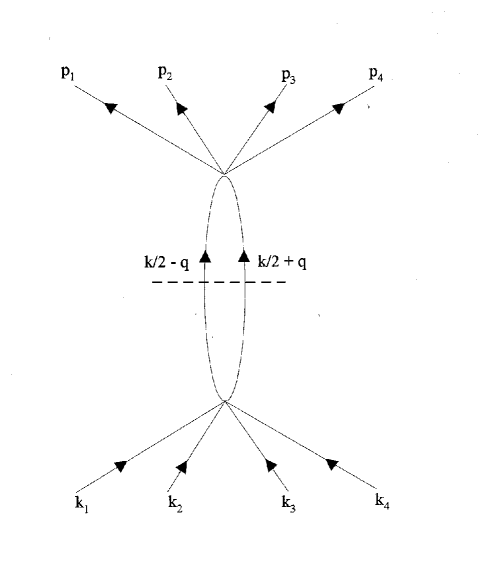
FIG. 1.: The order-$\lambda^{2}$ diagram in $\phi^{6}$ theory.

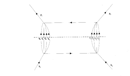
FIG. 2.: The order-$\lambda^{4}$ diagram in $\phi^{6}$ theory (the box diagram).

REFERENCES

• [1] R.Β R.Β Sastry, quant-ph/9903025.
• [2] M.Β E.Β Peskin and D.Β V.Β Schroeder, Introductory Quantum Field Theory, Addison-Wesley, 1995.
Refer to caption