A candidate for a background independent formulation of $\cal M$ theory

Lee Smolin^∗

Center for Gravitational Physics and Geometry

Department of Physics

The Pennsylvania State University

University Park, PA, USA 16802

March 10, 1999, revised Dec 26,1999

ABSTRACT

A class of background independent membrane field theories are studied, and several properties are discovered which suggest that they may play a role in a background independent form of $\cal M$ theory. The bulk kinematics of these theories are described in terms of the conformal blocks of an algebra $G_{q}$ on all oriented, finite genus, two-surfaces. The bulk dynamics is described in terms of causal histories in which time evolution is specified by giving amplitudes to certain local changes of the states. Holographic observables are defined which live in finite dimensional states spaces associated with boundaries in spacetime. We show here that the natural observables in these boundary state spaces are, when $G_{q}$ is chosen to be $Spin(D)$ or a supersymmetric extension of it, generalizations of matrix model coordinates in $D$ dimensions. In certain cases the bulk dynamics can be chosen so the matrix model dynamics is recoverd for the boundary observables. The bosonic and supersymmetric cases in $D=3$ and $D=9$ are studied, and it is shown that the latter is, in a certain limit, related to the matrix model formulation of $\cal M$ theory. This correspondence gives rise to a conjecture concerning a background independent form of $\cal M$ theory in terms of which excitations of the background independent membrane field theory that correspond to strings and $D0$ branes are identified.

^∗ smolin@phys.psu.edu

1 Introduction

In this paper a proposal is made for a background independent formulation of $\cal M$ theory[1]. This is based on a particular case of a general formulation for a background independent membrane field theory previously proposed with Markopoulou[2]. That work was, in turn, a natural extension of the spin network formalism that has been shown to characterize the exact gauge and diffeomorphism invariant states of a large class of theories of quantum gravity[3, 4, 5, 6, 7, 8], including supergravity[9, 10].

The spin network states are background independent, in the sense that they make no reference to any background metric or fields, because they result from an exact, non-perturbative quantization of the commutation relations of the gravitational fields. However, as they are constructed through a canonical quantization procedure, they do depend on the background topological and differential structure. As $S$ duality[1] and mirror manifolds[11] in string theory indicates the presence of symmetries mixing manifolds with different topology, this dependence must also be eliminated if one wants to construct a successful background independent form of $\cal M$ theory. In [2] it was shown that this can be accomplished simply by thickening the graphs which underlie the spin network states so that they become membranes. The labels on the spin networks are then replaced by the conformal blocks ${\cal V}_{g}$ of a chiral theory based on a quantum group or supergroup, $G_{q}$ for a two-manifold, ${\cal S}_{g}$ of genus $g$. The full space of states is then the conformal blocks of all compact oriented two-surfaces,

$${\cal H}=\sum_{g}{\cal V}_{g}.$$ (1)

In quantum general relativity[15, 16], in $3+1$ the level is proportional to the inverse cosmological constant,

$$k={6\pi\over G^{2}\Lambda}$$ (2)

As a consequence, the theory reduces to the spin network formalism in the limit that the cosmological constant, $\Lambda$, vanishes

Because the graphs of the spin network formalism have been thickened to two-surfaces, no embedding manifold need be assumed because there are states in $\cal H$ that carry appropriate information to construct both a manifold (of any dimension and topology) and the embedding of a two surface in it[2]. In fact, as we shall discuss below, what is naturally constructed are pseudomanifolds, whose defects may be the background independent analogues of branes[20].

In [18, 19] it was suggested that because of its resemblance to a background independent membrane theory, and the fact that such a theory may have a set of dynamically determined continuum limits which are classical spacetimes of different dimension and topology, an appropriately chosen member of this class of theories might be a background independent form of $\cal M$ theory. In [18] it was also shown that a theory of this kind can incorporate $SL(2,Z)$ string duality symmetry, leading to a non-perturbative description of string network states. In this paper a new connection between the background independent membrane theories described in [2] and string theory is reported, which leads to a proposal for a background independent form of $\cal M$ theory.

This new connection is the discovery of a certain class of observables, which are related to the coordinates of matrix model descriptions of membrane theory. As we will see, the bosonic matrix model in $D$ dimensions can be recovered when $G_{q}$ is chosen to be the quantum deformation of $Spin(D)$ and a certain choice of the dynamics is made. In certain cases this can be extended to a supersymmetric matrix model in $D$ dimensions, by exending $G_{q}$ to a superalgebra which has a $Spin(D)$ subalgebra. In the $9$ dimensional case relevant for the deWit-Hoppe-Nicolai-Banks-Fischler-Shenker-Susskind [21, 22] matrix model the appropriate superalgebra is, as we will discuss, $SU(16|1)$.

The natural physical interpretation of these observables which is suggested here is that they are the background independent versions of the coordinates of $D0$ branes. This is because we are able to argue that if the theory, in the form given below, has a semiclassical limit which is flat $11$ dimensional spacetime, those observables will indeed give the positions in the $9$ dimensional transverse space, defined by the light cone coordinates of a physical observer, of zero-dimensional objects on which strings end.

To see how this description emerges, it is necessary to understand the way in which the holographic principle is expressed in the background indepenedent theories described in [2]. In fact, the holographic principle, in a cosmological form discussed in [2, 24, 70], is a major part of the proposal made in [2]. As this theory has neither a background spacetime nor asymptotic or external regions, it is naturally cosmological. There is no place outside of the dynamical system for the observer to live. As was discussed in [23], in such a case all the observables of the quantum theory will be associated with closed surfaces that are dynamically embedded in the spacetime. These observables describe what an observer living on the surface could measure about the physics on its interior. These surfaces will play a major role in this paper, they will be referred to as holographic surfaces.

As there is no asymptotic region, the areas of these surfaces will be generally finite. By the Bekenstein bound[25], the state spaces on which these boundary observables act must have finite dimension, proportional to the exponential of of the area, in Planck units. In [16, 26, 27] it was shown that, at least in the cases of quantum general relativity and supergravity, with a non-zero cosmological constant, this condition is met.

In these theories the boundary state spaces are naturally spaces of intertwiners (or conformal blocks) for $G_{q}$ on punctured surfaces, with the punctures representing points where excitations of the quantum geometry in the interior may end. It is these punctures which are identified with $D0$ branes. To explain why, it is necessary to understood how dynamics is formulated in this theory.

The main idea is that the dynamics is given in terms of a causal histories framework, first proposed for quantum gravity in [30]. In this kind of theory, a history, $\cal M$, is constructed from a given initial state by a series of local evolution moves. These resemble the bubble evolution in general relativity and as a result, these histories have a natural analogue of the causal structure of general relativity. This makes it possible to identify the analogues of light cones, horizons, spacelike surfaces and many-fingered time precisely at the quantum level, prior to any continuum limit being taken.

The dynamics is specified by the choice of local moves and the amplitudes that are assigned to them. Thus, in this kind of theory a new kind of fusion between quantum theory and spacetime is achieved in which states are identified with quantum geometries that represent spacelike surfaces, and histories are both sequences of states in a Hilbert space and discrete analogues of the causal structures of classical spacetimes.

The connection with string theory arises because small perturbations of states are parameterized by closed loops drawn on the two surfaces ${\cal S}_{g}$ [35]. The small perturbations of a history $\cal M$ are then in one to one correspondence with the embeddings of certain time like combinatorial two dimensional surfaces in $\cal M$. As argued in [35], if the theory has a classical limit then the amplitudes for these perturbations must reproduce the actions for excitations of string worldsheets.

When such an excitation takes place within a surface associated with a holographic observer, it can end on one of that surface’s punctures. Thus, the punctures are structures on which strings end, which is to say they are $D0$ branes. The question is then to discover the observables that describe the configurations of the $D0$ branes, and to deduce their effective dynamics.

The holographic principle, in the background independent form proposed in [2, 70], plays a central role in achieving this. There is a natural correspondence between bulk and boundary states, which is suggested by topological quantum field theory[36], and confirmed in the case of quantum general relativity[16, 26] and supergravity[27], with a cosmological constant. This is that the hamiltonian constraint, which codes the spacetime diffeomorphism invariance, is satisfied by the application of recoupling identities of quantum groups on the quantum states of the theory. In a histories, rather than a canonical theory, this must be imposed in a way which is consistent with causality, so that information is not propagated from the bulk to the boundary faster than the causal structure of the quantum spacetimes allowed. Below, in section 3, we will see how to do this.

Once the map between bulk and boundary states is understood, the next step is identifying the holographic observables that describe the boundary states, and giving them a physical interpretation. A clue for how to do this comes from Penrose’s original work on what he called the spin-geometry theorem[37]. This theorem associates to generic, large, spin networks with $N$ free ends an assignment of $N$ points on an $S^{2}$. We show here that a similar result is true in any dimension, and that this implies that the observables which describe the punctures/$D0$ branes in the present theory are closely related to those of a matrix model. In the case that $G_{q}$ is $Spin(D)$ or an appropriate supersymmetric extension of it we find that the observables associated with a surface with $N$ punctures then corresponds to a matrix model in $D$ dimensions.

This paper is divided into $11$ sections. The next is devoted to an exposition of background independent membrane field theory[2, 18] in the causal histories formulation of Markopoulou[30]. Enough detail is given, and the basic concepts are stressed, so that no prior knowledge of loop quantum gravity need be assumed.

Section 3 is then devoted to certain conceptual and technical points regarding the treatment of gauge and diffeomorphism invariance in this class of theories. This is necessary preparation for the main work of the paper, which is the uncovering of the relationship to string theory. We begin this in section 4 where we review the results of [35] that show that small perturbations of the states are described by loops embedded in the quantum geometry so that small perturbations of causal histories are associated with embeddings of combinatorial time like two surfaces in the histories. This leads us in section 5 to the identification of punctures on the holographic surfaces where strings may end as $D0$ branes.

In section 6 we identify observables that code the dynamics of these punctures and show that they are closely related to those of the matrix model. We then show that in $D=3$ there is a surprising relationship between the observables that describe the $D0$ branes and Penrose’s original spin network formalism [37]. This suggests a certain simplification of the operators that represent the $D0$ brane dynamics.

Finally, in section 7-10 we show that the bulk dynamics may be chosen so that the dynamics of the punctures which is induced by the bulk-to-boundary map reduces, in the appropriate limits, that given by the matrix models. The bosonic and supersymmetric matrix models in $D=3$ are studied in sections 7 and 8; in 9 and 10 we study their counterparts in $D=9$. The main results of the paper are then summarized in the concluding section. These are the basis of three conjectures we then state, which concern the form of the background independent form of $\cal M$ theory. We also discuss there several implications of the conjecture, which should be explored in future work. The most important of these is that there are consequences for the $AdS/CFT$ conjecture[38, 39, 40]. If both that and the present conjecture are true, than we can deduce the exact form of the Hilbert spaces and operator algebras for the boundary conformal field theories in $AdS$ spacetimes. Similarly, there are consequences for counting states of black holes.

2 Background independent membrane field theory

In this section we summarize the general structure defined in [2], and the motivation coming from results in both string theory and in quantum general relativity and supergravity. For more details the reader is referred to [2, 18, 30].

2.1 The kinematics of background independent membranes

We would like to describe a class of membrane theories in which the embedding space has no prior existence, but is instead coded completely in the degrees of freedom that live on the two surfaces. As the background is not assumed to exist a priori, there are no embedding coordinates. Instead, the kinematical structure is given by the choice of a quantum group or supergroup $G_{q}$ where $q$ will be assumed to be taken at a root of unity. $G_{q}$ has a finite list of finite dimensional representations, which will be labeled $j,k,l\ldots$.

Using standard constructions from conformal field theory[41, 42, 43, 44] or representation theory[45] there is associated to each oriented closed two-surface $\cal S$ of genus $g$ a finite dimensional space ${\cal V}^{g}$, which is called the space of conformal blocks of WZW theory based on $G_{q}$. The surface may also be punctured, which means that there are a set of $N$ marked points, labeled by a set of representations, $\{j\}$ of $G_{q}$. The same construction yields a finite dimensional vector space ${\cal V}^{g,N}_{\{j\}}$. When the manifold is $S^{2}$, ${\cal V}_{\{j\}}^{S^{2}}$ is called the space of intertwiners.

These spaces may be constructed in the natural way described in [41, 43, 44] from ${\cal V}^{S^{2}}_{jkl}$, which is called the trinion. An arbitrary surface is constructed by joining three punctured spheres at labeled circles, taking the direct product of the ${\cal V}^{S^{2}}_{jkl}$ over all the three-punctured spheres and summing over labels. Every way of decomposing $\cal S$ in terms of trinions yields a basis of ${\cal V}^{\cal S}$, where the basis elements are labeled by the circles and intertwiners.

Figure 1: A trinion which represents the intertwiner of three representations of $G_{q}$.

The full state space of the theory is defined to be

$${\cal H}=\bigoplus_{g}{\cal V}^{g}$$ (3)

As this is the fundamental assumption of this theory, let us take a moment to stress it. It means that the fundamental things that the world is composed of are only systems of relations, involving nothing but the multiplication and decomposition of representations of some fundamental algebra $G_{q}$. At the fundamental level, spacetime is nothing but a coarse grained description of processes in which these systems of relations evolve. There is no background geometry or topology, nor are there fields, particles, strings or branes that move in them. These must emerge from the kinematics and dynamics of the states in $\cal H$.

2.2 How quantum geometry is coded into conformal blocks

Let us begin with geometry. It may seem that this arena is too poor to describe quantum geometry. However, this is not the case. There are in fact bases of states in $\cal H$, whose elements may be associated in an a natural way with quantum geometries of $d$ dimensions, for any $d$. The construction for $d=3$ is particularly simple[2], I discuss it in detail and then briefly mention describe the extension to larger dimension.

$d=3$ pseudomanifolds from conformal blocks

We consider, for large $g$, a decomposition of the genus $g$ surface, ${\cal S}^{g}$ into a number, $P$, of $4$-punctured spheres. We label these $B_{d}^{i}$, with $i=1,\ldots,P$. The decomposition is achieved by cutting ${\cal S}_{g}$ along a number, $N$, of circles which we will label $c_{\alpha}$, with $\alpha=1,\ldots,N$. We can represent the decomposition by a $4$-valent framed graph $\Gamma$, with $P$ nodes representing the $B_{d}^{i}$ and $N$ edges representing the circles $c_{\alpha}$ (See Figure (2).). An associated basis of states in ${\cal V}^{g}$ is given by assigning a representation $j_{a}$ of $G_{q}$ to each circle $c_{\alpha}$ (or edge of $\Gamma$) and assigning a basis in the space of $4$ intertwiners $\mu_{i}$ to each $B_{g,d}^{i}$, (or node of $\Gamma$). These basis elements may then be labeled $|\Gamma,j_{a},\mu_{i}>$. Given such a choice of basis for each $g$ yields a basis for all of $\cal H$.

Figure 2: A simple example of two surface, and its dual graph $\Gamma$.

Now to each element, $|\Gamma,j_{a},\mu_{i}>$, of this basis we may associate a dual $3$ dimensional pseudomanifold ${\cal E}|\Gamma,j_{a},\mu_{i}]$. Dual to each node of $\Gamma$ we construct a $3$ simplex, with $2$ dimensional “faces” that correspond to the $4$ edges incident on it. Tying the faces together, following the framing that follows from the orientation on the surfaces, one constructs a simplicial pseudomanifold of $3$ dimensions, whose faces are labeled by the representations $j_{a}$ and whose simplices are labeled by intertwiners. (For a simple example, see (3).)

Figure 3: A simple example of two surface, divided into four punctured spheres. The dual $3$-manifold is the boundary of the four-simplex.

The pseudomanifold ${\cal E}|\Gamma,j_{a},\mu_{i}]$ inherits the labeling from the state $|\Gamma,j_{a},\mu_{i}>$. The faces are labeled by the representations $j_{\alpha}$ and the simplices by the intertwiners $\mu_{i}$. We may give these a geometrical interpretation, which is motivated by the results of quantum general relativity in $3+1$ dimensions[7, 5, 6, 50]. To each representation $j_{\alpha}$ we may assign a quanta of $d-1$ dimensional area, given by

$$A[j_{\alpha}]=l_{Planck}^{d-1}\sqrt{C[j_{\alpha}]}$$ (4)

where $C[j_{\alpha}]$ is the quadratic Casimir of $G_{q}$. This matches the result of the computation of the area operator in quantum general relativity[5, 6] and supergravity[10] in $3+1$ dimensions. In those cases the operator for the volume of a simplex was also computed and found to be given by a finite, positive hermitian operator $\hat{Vol}$ on ${\cal V}_{j_{1},j_{2},j_{3},j_{4}}^{S^{2}}$.

For a general $G_{q}$ we must make choices of area and volume operators, the first of which are functions of the representations, $j$ the second of which are positive operators on the ${\cal V}_{j_{1},j_{2},j_{3},j_{4}}^{S^{2}}$. While these may be suggested by the results from canonical quantum gravity, there is no need they be chosen so, and they may be chosen for a general $G_{q}$. Once choices of the area and volume operators are made, the labeled pseudomanifold ${\cal E}|\Gamma,j_{a},\mu_{i}]$ has a geometrical interpretation in terms of volumes and areas.

The statement that the states in $\cal H$ are naturally associated with pseudomanifolds means that the simplicial manifold dual to a state $|\Gamma,j_{a},\mu_{i}>$ may or may not be consistent with the application of the manifold conditions on the simplices of dimension $0$ and $1$. This means that a general state $|\Gamma,j_{a},\mu_{i}>$ can be associated with a $3$ dimensional geometry, but one with defects of dimensions$0$ and $1$. In some cases these defects resemble orientifolds, in that they may arise from a combinatorial manifold by identification of lower dimensional simplices. When considered in isolation, these identified surfaces will behave as defects, inheriting dynamics from the fundamental dynamics on $\cal H$. These must be considered to be an inherent part of the theory; I will argue in the conclusion that at least in some cases the higher dimensional analogues of these may give rise to the $D$-branes.

We will also need to be able to talk about quantum geometries with boundaries. These are described by states that live in the spaces of conformal blocks associated with punctured surfaces, which we denoted ${\cal V}^{g,m}_{j_{a}}$. We may also consider the space of all states with the same boundary, given by

$${\cal H}^{m}_{j_{a}}=\bigoplus_{g}{\cal V}^{g,m}_{j_{a}}.$$ (5)

The $d=4$ case

The key point in the above construction was to associate a $3$-simplex as a region $\cal R$ of a two-surface $\Sigma$, with its connections to its $4$ neighbors across its $4$ triangles associated to a set of labeled punctures, $c_{i}$ which, when cut, separate $\cal R$ from $\Sigma$. For the case $d=3$ it is natural to take $\cal R$ to have genus $0$. The reason for this choice is that each puncture can be associated to a region of $\cal R$, each of which bounds all the others. The meaning of this is that the dual skeleton of the surface of the three simplex can be drawn on $\cal R$ in such a way that its nodes are at the punctures and the edges that connect each pair of nodes are represented as lines that join the punctures. We may note that these lines may be themselves labeled with representations to give an intertwiner or conformal block on the four-punctured sphere.

When we go up to $d=4$ we want to represent $4-$simplices by regions $\cal R$ of a two surface, with $5$ punctures, each labeling a $3$-simplex that is shared between this four simplex and its neighbors. $\cal R$ should have thus have the topology of a $5$ punctured surface, with the property that each puncture can be surrounded by a region of $\cal R$, such that each of the five regions shares a border with each of the other four. The minimal genus for $\cal R$ is then $1$ because the torus is the lowest genus on which five colors can be required for coloring a map.

We may now repeat the above construction. We need operators to represent $3$-area and $4$-volume. The former must be a positive function of the representation labels, $j$, while the latter must be a positive operator in ${\cal V}^{g=1}_{j_{1},\ldots.,j_{5}}$ symmetric in all labels, for each set $j_{1},\ldots,j_{5}$. Given $V$ we then label a basis of states in each ${\cal V}^{g=1}_{j_{1},\ldots.,j_{5}}$ by a set of eigenvalues $v^{i}$. (If these are degenerate they can be supplemented by other geometric operators.).

For $G_{q}$ related to $SO(4)$ or a supersymmetric extension of it, these operators can be derived from a canonical quantization of $4+1$ dimensional general relativity or supergravity. This has not yet been done, but there is no reason it should not exist. In any case, all that is required for the present construction is a choice of of area and volume operators for the group $g_{q}$

We now proceed to associate labeled $4$-pseudomanifolds to conformal blocks of high genus surfaces by following the construction for $d=3$. Given a very large genus surface, ${\cal S}^{g}$ with $g$ chosen so it can be decomposed into a number $P$, of $5$-punctured torus’s, which are called $T^{i}$, with $i=1,\ldots,P$. We fix such a decomposition, which is achieved by cutting ${\cal S}_{g}$ along a number, $N$, of circles which we will label $c_{\alpha}$, with $\alpha=1,\ldots,N$. The sets of eigenvalues $(v^{i},a^{\alpha})$, then label a basis of states $|(v^{i},a^{\alpha})>$, in ${\cal V}^{g}$. To each such state we associate a labeled pseudomanifold by the following construction. We construct it from $P$ $4$-simplices, $S^{i}$, each corresponding to a $T^{i}$. Each is attached to $5$ others along the circles $c_{\alpha}$. This gives us a $4$ dimensional pseudomanifold which is associated to the decomposition (and hence the choice of basis in ${\cal V}^{g}$). To each $4$-simplex we associate the four volume given by the eigenvalue $v^{i}$ and to each $3$-simplex the three area given by the eigenvalue $a_{\alpha}$. The result is a $4$ dimensional pseudomanifold, each of whose $3$ and $4$ dimensional simplices has been assigned a volume.

The construction works in reverse as well, given a $4$ dimensional pseudomanifold, whose $N$ $3$-simplices and $P$ $4$-simplices are labeled by eigenvalues in the spectra of the $3$-area and $4$-volume operators, we can construct a two surface ${\cal S}^{g}$ for some $g$, by gluing together $P$ $5$-punctured tori. The correspondence between labels on the pseudomanifolds and states in the spaces of intertwiners on the $5$-punctured tori yields a state in ${\cal V}^{g}$.

2.3 The general case

To generalize the construction to general $d$ we must choose the genus of the regions $\cal R$ such that it can be divided into $d+1$ regions, each of which shares a boundary with each of the others. These will have at least genus $d-3$. Each of the $d+1$ regions is then punctured and the punctures on neighboring regions are joined. To complete the construction one needs to find the appropriate volume and area operators, presumably from a canonical quantization of supergravity in the appropriate dimension.

Finally, we may note that different bases are associated with different geometrical decompositions of $\cal H$, of different dimension $d$. This means that the dimension as well as the topological and metric properties of the associated quantum geometry are dynamical quantities, they are determined completely by the states. Which dimension, topologies and geometries emerge in the classical limit is a dynamical problem. We may also note that superpositions of states that give rise to an interpretation in terms of a $d$ dimensional quantum geometry will in certain cases be interpretable as states associated with quantum geometries of dimensions $d^{\prime}\neq d$.

These are all features that we would expect of a truly background independent quantum theory of gravity.

2.4 Reduction to quantum general relativity and supergravity

Quantum general relativity and supergravity, with a cosmological constant, $\Lambda$, provide prototypes for the class of theories just described. In the Euclidean case, $G_{q}=SU(2)_{q}$ for general relativity and $G_{q}=SU(2|{\cal N})_{q}$ for supergravity, for $\cal N$ at least up to $2$. The quantum deformation is given by the cosmological constant, with $q=e^{2\pi\imath/k+2}$, with the level $k$ given by (2). The main results here are based on the existence of a closed form expression for the vacuum state, which is given by[12],

$$\Psi_{CS}(A)=e^{{3\over G^{2}\Lambda}\int Y(A)_{CS}}$$ (6)

where $Y(A)_{CS}$ is the Chern-Simons invariant of the Sen-Ashtekar connection[13, 14]. A lot is known about this sector of the theory[48, 49], including the fact that the semiclassical behavior is that of small fluctuations around deSitter or anti-deSitter spacetime[12, 15]. The supersymmetric extensions are also known[9]. An important fact is that the observables algebra of this theory requires that the spin networks be quantum deformed[17], as described in [45].

In the case of a spacetime with boundary, a class of boundary conditions has been studied in which Chern-Simons theory is induced on the boundary[16]. With $\Lambda\neq 0$ there is a class of exact solutions to the quantum constraints, labeled by the conformal blocks for all the possible choices of punctures on the spatial boundary; the number of these solutions is consistent with the Bekenstein bound[16].

Similar results have been found also in the Lorentzian case[26], in which case $G^{q}=SU(2)_{q}\otimes SU(2)_{q}$, where, however the representations and intertwiners are restricted by the balanced condition $j_{left}=j_{right}$, first proposed in [47].

Finally, we note that when we take $\Lambda\rightarrow 0$ this implies, by (2, that $q\rightarrow 1$ so that the states reduce to ordinary spin networks[45, 17]. Quantum general relativity in this limit has been studied in great detail [3, 4, 5, 6, 7, 8, 48, 49, 50], and the results found have been verified by rigorous theorems[51, 52, 53, 54].

2.5 Holographic observables

There are several lines of argument that point to the conclusion that in a quantum theory of gravity, all observables should be associated with boundaries, of dimension, in the continuum limit, $1$ less than the spatial dimension. These include the arguments for the holographic hypothesis of ‘t Hooft[55], whose relevance for string theory has been argued by Susskind[56]. We know from several examples that the holographic principle may be satisfied in a quantum theory of gravity, although its exact formulation, for cosmological theories, remains controversial[57, 58, 24, 69].

There are a parallel set of arguments in the literature on quantum gravity and cosmology, put forward originally by Crane[36], and continued in [23, 61, 62, 63, 64, 65, 70], to the effect that observables in a cosmological theory must be associated with a splitting of the universe into two pieces. According to this point of view, such a splitting may correspond to a situation in which a subsystem of the universe, delineated by the boundary, is studied by observers who are able to make measurements only on the boundary. One may then set up what is called a relational[61] or pluralistic[23, 62] quantum cosmology in which there is a space of states and an observable algebra associated to every possible such spatial boundary. These different state spaces are tied together by linear maps whose structure is determined by a functor from the category of cobordisms of $d-1$ dimensional surfaces[36, 23]. This is done in such a way that the Hilbert space associated to the whole universe is always one dimensional, making it impossible to construct any non-trivial observables associated to the universe as a whole. Given that no observers have access to the entire universe, this is argued in [36, 61, 23, 62, 63, 64, 65, 70] to be a necessary property of a realistic quantum theory of cosmology.

In the present setting we can realize this approach to holographic observables by associating algebras of observables with different ways of splitting the two-surfaces into two parts, each representing different halves of a quantum geometry, split along a boundary. This is done in the following way. Given a quantum state, $|\Gamma,j_{a},\mu_{i}>$ cut the surface ${\cal S}_{g[\Gamma]}$ along any subset of $N$ of its circles $c_{a}$ which results in the splitting of ${\cal S}_{g}$ into two pieces, which we will call ${\cal S}_{g}^{\pm}$. The splitting introduces an abstract surface, which may be taken to be a punctured $S^{2}$, with $N$ punctures. These punctures inherit the labels $j_{a}$ on the $N$ circles.

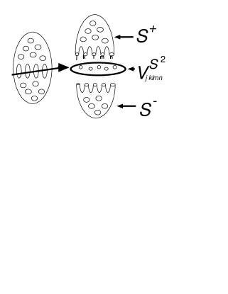
Figure 4: A quantum geometry $|\Gamma,j_{a},\mu_{i}>$ is cut along $5$ circles, yielding two bounded quantum geometries, ${\cal S}_{g}^{\pm}$, which meet on a boundary which is represented by a $5$-punctured $S^{2}$.

${\cal S}_{g}^{\pm}$ are each a quantum geometry with boundary constructed from the graph dual to ${\cal S}_{g}^{\pm}$. It is interesting to ask how the boundary is described in the picture described above, in which there are bases of states which have a dual description in terms of a labeled $d$ dimensional combinatorial pseudomanifold. In this picture, the pseudomanifold must have a $d-1$ dimensional boundary, $\partial{\cal S}_{g}^{\pm}$ which is composed of $N$ $d-1$ dimensional simplices, labeled by the $j_{a}$. In a continuum limit, this surface will correspond to a $d-1$ dimensional surface which divides space into two parts.

According to the holographic principle, the physical information that observers living on the boundary $\partial{\cal S}_{g}^{\pm}$ may gain about ${\cal S}_{g}^{+}$ must then be represented in terms of a field theory on the boundary. There is a state space naturally associated with that boundary, which is ${\cal V}_{j_{a}}^{S^{2}}$. The algebra of observables on ${\cal V}_{j_{a}}^{S^{2}}$ then contains all the information that observers may learn about the interior ${\cal S}_{g}^{+}$ by measurements made on the boundary.

This picture is realized in quantum general relativity [16, 23, 26], for the case of non-vanishing cosmological constant.

We may note that for finite numbers of punctures, the dimension of the boundary state space ${\cal V}_{j_{a}}^{S^{2}}$ is finite, even as $q\rightarrow 1$. In quantum general relativity, this is consistent with the Bekenstein bound, because the area of the boundary is given by $l^{2}_{Pl}\sum_{\alpha}\sqrt{C(j_{\alpha})}$ [16].

Note that we have defined two different surfaces that are associated with the boundary. There is the $2$ dimensional surface, which is the punctured $S^{2}$ on which the boundary state space, ${\cal V}_{j_{a}}^{S^{2}}$, lives. Then there is the $D-1$ dimensional pseudomanifold, $\partial{\cal S}_{g}^{\pm}$. For $D=3$, these surfaces coincide, the latter gives a simplicial description of the punctured $S^{2}$, with a puncture inside each triangular face. However, for $D>3$ they are different. The construction of the dual pseudomanifold will give us an embedding of the $S^{2}$ in the combinatorial pseudomanifold $\partial{\cal S}_{g}^{\pm}$. In the limit of a large number of punctures, this must go over into the embedding of a $2$-brane in the $D-1$ dimensional boundary. This $2$-brane is made of $0$-branes, which are the punctures in the surface. This is the basis of the correspondence to $\cal M$ theory we will develop below.

To develop this picture we must have a clear understanding of how the holographic principle is realized in this background independent context. The main mystery of the holographic principle may be stated in this context as follows. The state space of a finite area boundary must be finite dimensional, by the Bekenstein bound. However, there seems to be an infinite dimensional space of possible states for the fields in the interior. The problem is how the reduction from a potentially infinite number of bulk states to a finite dimensional space of states, observable on the boundary, is achieved. In the present case, the theory must provide a map $\Phi$ which reduces the infinite dimensional space of bulk states, ${\cal H}^{N}_{j_{a}}$, to the finite dimensional space of boundary states, ${\cal V}_{j_{a}}^{S^{2}}$. There is a natural proposal for this map[2, 36] which is motivated by the results of quantum general relativity and supergravity with finite $\Lambda$ [16, 26]. This is that the map is given by Chern-Simons theory. A state $|\Gamma,j_{a},\mu_{i}>\in{\cal H}^{N}_{j_{a}}$ corresponds to a framed $G_{q}$ spin network with $N$ open ends, with labels $j_{a}$. By standard constructions[42, 43, 45] it can be read as an $N$-intertwiner for $G^{q}$ and hence as an element of ${\cal V}_{j_{a}}^{S^{2}}$. We denote the resulting linear map by

$$\Phi:{\cal H}^{N}_{j_{a}}\rightarrow{\cal V}_{j_{a}}^{S^{2}}.$$ (7)

In these cases we will use the tilde to denote

$$\Phi\circ|\Psi>\equiv|\tilde{\Psi}>\in{\cal V}_{j_{a}}^{S^{2}}$$ (8)

This choice is motivated by results from quantum general relativity and supergravity in $3+1$ dimensions. In the canonical formalism of quantum gravity and supergravity, the map $\Phi$ is is realized as the loop transform [4] of the Chern-Simons state (6) in the presence of boundary states given by conformal blocks of the punctured boundary. The details of this are described in [16]. One way to say this is that there is a sector of states in which the Hamiltonian constraint of quantum general relativity (and supergravity) is equivalent to the recoupling relations of framed $SU(2)_{q}$ (or $SU(2|1)$) spin networks[16, 17, 10]. What we are going to do is use the natural extension of this result to define the relationship between the bulk and surface states in $\cal M$ theory.

In a histories formalism of the kind we will use here, the definition of the map will have to be supplemented by giving time slicings of both the boundary and the interior. We will be able to do this after we have explained how histories are constructed in this theory.

2.6 The form of the local evolution operator

We now turn to the dynamics given to these background independent membrane field theories. For reasons given in [2] we describe the dynamics in terms of a causal histories framework, first proposed for quantum general relativity in [30]. In this approach the dynamics is given by a set of local replacement moves. In each such move a specified $m$- punctured surface ${\cal S}_{past}$ is removed from the surface $\cal S$. This results in $m$ free ends, with labels $j_{\alpha}$. A new surface with matching labels, ${\cal S}_{future}$ is then inserted in its place. (See Figure (5).) This corresponds to the removal of a state $|past>$ in ${\cal H}^{m}_{j_{a}}$ and its replacement by a state $|future>$. Given a choice of operator $\hat{h}$ in each ${\cal V}_{j_{a}}^{S^{2}}$ and using $\Phi$ to associate $|past>$ and $|future>$ to states in ${\cal V}_{j_{a}}^{S^{2}}$, the amplitude for each such move is given by

$${\cal A}(move)=<\tilde{future}|\hat{h}|\tilde{past}>.$$ (9)

Figure 5: An example of a substitution move. Histories $\cal M$ are made up of successive applications of such moves.

A causal history, $\cal M$ is specified by the choice of an initial state, $|0>=|\Gamma,j_{a},\mu_{i}>\in{\cal H}$, followed by a sequence $I=1,2,3,\ldots$ of substitution moves. The result is a sequence of states, $|0>,|1>,\ldots,|I>$, each resulting from the previous one by a substitution move.

The amplitude for a history is then given by the product

$${\cal A}[{\cal M}]=\prod_{I}{\cal A}(I)$$ (10)

The dynamics is then defined conventionally by summing over all histories between given initial and final states.

As the substitution rules are local, this results in a structure which is in many ways analogous to a continuous Lorentzian spacetime[30, 2]. Just as a classical spacetime may be constructed from a given initial surface by a series of local, “bubble evolution” steps, in which the spatial hypersurface is evolved within a compact region, a causal history $\cal M$ may be seen as a spacetime structure generated by local evolution moves on a state representing a quantum spacelike surface.

The precise way to describe this is to note that $\cal M$ has the structure of a causal set $\cal C$ [30, 2]. To each of the regions removed or inserted by a substitution move, one associates an element $q\in{\cal C}$. A partial ordering may be defined on $\cal C$ as follows: $p>q$ if there is a series of substitution moves that begins with the removal of $q$ and ends with the insertion of $p$, such that in each step the set removed overlaps the set inserted in the previous move. It is then easy to see that $\cal C$ has the structure of a causal set. We call it ${\cal C}[{\cal M}]$.

The causal set ${\cal C}[{\cal M}]$ gives to $\cal M$ discrete analogues of many of the properties of Lorentzian spacetimes, such as many fingered time, light cones, and horizons[30, 2]. Various aspects of this are described in more detail in [30, 63, 2, 20]. We may note that the association of fundamental quantum histories with causal structures and quantum states with quantum geometries makes this class of theories generalizations of both general relativity and quantum theory. Each history $\cal M$, is both a sequence of states in a Hilbert space, ${\cal H}$, defined without reference to any background structure and a causal structure which shares many properties with a Lorentzian spacetime.

This ends the summary of the class of background independent membrane theories proposed in [2]. To summarize, a member of this class of theories is given by the following choices:

• 1) The algebra or superalgebra, $G_{q}$.

• 2) The choice of substitution moves used in the evolution.

• 3) The choice of the operators $h$ that give the amplitudes for the causal histories $\cal M$.

Particular choices have been suggested for the theory corresponding to quantum general relativity in the Euclidean [46, 47] and Lorentzian[30] case. (See Figure (6)). The question that we may now address is whether there are any choices that give continuum limits described by string theory.

Figure 6: Examples of past/future pairs that are used in the substitution moves in quantum general relativity. These come from cuts of the thickened four simplex.

3 Consequences of a Planck scale causal structure

There are several important issues we must clarify, before we go on to study the possible relationship with string theory.

3.1 The continuum limit

The most important physical question regarding the class of theories we have just defined is whether there exists for any of them a continuum limit which reproduces classical general relativity in some dimension, coupled to some set of quantum fields. The main conjecture we are pursuing in this line of work is that if any of these theories has a continuum limit, there must be a consistent description of small perturbations around that limit, and this in turn must reproduce a string perturbation theory, because there is strong evidence that all successful perturbative gravitational theories are string theories. The main question, to be discussed below, is then how to construct observables of the fundamental theory that will describe these string-like, perturbative degrees of freedom, when the continuum limit exists.

We will return to the problem of the continuum limit in the conclusions. This is the main question that we will not be able to solve in this paper.

3.2 Spacetime diffeomorphisms, gauge fixing and discrete causal structure

To discuss the issue of gauge invariance we need some language to describe a causal set. Given the causal set ${\cal C}[{\cal M}]$ we can define an acausal set to be a set of elements $q_{i}\in{\cal C}[{\cal M}]$ such that there are no causal relations amongst them. An antichain $A$ is a maximal acausal set, which means that no $p\in{\cal C}[{\cal M}]$ can be added to $A$ without violating the condition that it be an acausal set[63, 64].

A time slicing ${\cal T}=A(t)$ for $t=0,1,2,\ldots$ is a sequence of antichains such that every $p\in{\cal C}[{\cal M}]$ is in some $A(t)$. This is just like a time slicing in general relativity, except that the time parameter is discrete.

As in general relativity, there are many possible slicings of a history. These may be distinguished by gauge conditions. Whenever we refer to a slicing we will have to give conditions that pick it out.

This is especially important when we come to the description of physical time evolution. In general relativity the Hamiltonian on the physical, gauge invariant, state space is a function of the fields on the boundary. To give the correct interpretation of the present setting, which insures that if there is a classical limit it will go over to the correct description of evolution in the classical theory, we must ask whether the local evolution moves are physical or gauge. This is an issue because in general relativity the Hamiltonian constraint generates both changes in the time coordinate and local evolution moves.

In the kinds of theories defined in [30, 2] the local evolution moves generate physical evolution because the causal set ${\cal C}[{\cal M}]$ corresponds to the causal structure of spacetime. Thus the past set and future set in a single local evolution move must correspond to physically different sets of events, because they have different causal relations with the other events, and this corresponds in the classical theory to distinct physical spacetime events. Another way to say this is that the causal set associated to a history in general relativity is a spacetime diffeomorphism invariant. As such, the causal set ${\cal C}[{\cal M}]$ of a discrete quantum history is also a gauge invariant description that, in the classical limit, (if one exists) must correspond to the spacetime diffeomorphism invariant causal set of a Lorentzian spacetime.

One consequence of this is that, unlike the case of state sum models of topological quantum field theories, the sum over histories is NOT a projection operator. This is because there is no history where nothing happens to the states. Every history is a sequence of real changes to the states and these then correspond to a spacetime invariant description of real events.

This does not mean that states must not satisfy additional conditions, corresponding to the conditions on initial data in the classical theory. But these conditions are different from the sum over histories, as each quantum history must correspond, in the case that there is a classical limit, to a spacetime diffeomorphism invariant description of a classical history.

3.3 Slicing conditions in the bulk and on the boundary

There are special issues, in both the classical and quantum theory, when a finite boundary has been introduced. Note that to every antichain $A\in{\cal C}[{\cal M}]$ is associated a state $|A>\in{\cal H}^{N}_{j_{a}}$. Thus to a time slicing $A(t)$ is a sequence of states $|A(t)>\in{\cal H}^{N}_{j_{a}}$. By (7) this induces a sequence of states $|\tilde{t}>\in{\cal V}_{j_{a}}^{S^{2}}$.

The question is then which slicing in the bulk is to correspond to a choice of slicing on the boundary. There is a unique answer which is dictated by causality. Given a history $\cal M$ with boundary and a time slicing $\tilde{t}$ on the boundary, we define the maximally past slicing, $A(\tilde{t})$, to be one that agrees with $\tilde{t}$ on the boundary and is past inextendible in the interior. This means that for each slice $A(\tilde{t})$, which is an antichain in the interior, there is no past replacement move, which would remove a connected subset $a\subset A(\bar{t})$, disjoint from the boundary, and replace it with elements $a^{\prime}$ such that,

1) $a^{\prime}<a$ in $\cal C$, and

2) $(A(\bar{t})-a)\cup a^{\prime}$ is an antichain.

Conceptually, such a slicing is one in which each spatial slice is as close to the past lightcone of a given slice of the boundary as it can be and still be a complete spacelike slice. It is not difficult to argue that for bounded histories $\cal M$ of the kind defined here, given a slicing of the boundary, such a slicing of the interior can always be chosen.

It is interesting to note that in the continuum limit the slice approaches the past light cone of the cut of the boundary. Thus, when $\Lambda<0$ the limit that the boundary is taken to infinity should reproduce the $AdS/CFT$ correspondence. It is also intriguing to note that when $\Lambda=0$ this description must reproduce the heaven description of Newman and collaborators[59] in which solutions to Einstein’s equations are described completely in terms of data on cuts of ${\cal I}^{+}$.

Given such a slicing we then have a sequence of states $|{t}>\in{\cal H}^{N}_{j_{a}}$. By the holographic map, eq. (7) this will induce a sequence of states $|\tilde{t}>$ in the boundary state space ${\cal V}_{j_{a}}^{S^{2}}$ given by

$$|\tilde{t}>=\Phi\circ|t>$$ (11)

As a consequence, there must be a time evolution operator $\hat{U}(t,s)$ on ${\cal V}_{j_{a}}^{S^{2}}$ such that

$$|\tilde{t}>=\hat{U}(t,s)|\tilde{s}>$$ (12)

We will be concerned to identify this operator. To do so, we need to identify a set of operators in ${\cal V}_{j_{a}}^{S^{2}}$ which we may use to understand the dynamics of the induced boundary states $|\tilde{t}>$. To do this it is helpful to have a physical interpretation for the information in the boundary state space ${\cal V}_{j_{a}}^{S^{2}}$. As we now show, a very interesting interpretation is suggested by studying the properties of the small perturbations around bounded histories.

4 Small perturbations, and the identification of string world sheets

Now that we have cleared away some technical and conceptual issues, we are ready to come to the heart of the matter, which is the identification of small perturbations of a history $\cal M$ with string worldsheets embedded, in a suitable sense, in $\cal M$.

Let us begin by considering an arbitrary history and asking what small perturbations look like. A history is a sequence of states $|I>=|\Gamma^{I},j_{a}^{I},\mu_{i}^{I}>$ each generated from the previous one by a local move. Thus, a perturbed history $|I^{\prime}>=|\Gamma^{I^{\prime}},j_{a}^{I^{\prime}},\mu_{i}^{I^{\prime}}>$ will involve a series of states $|\Gamma^{I^{\prime}},j_{a}^{I^{\prime}},\mu_{i}^{I^{\prime}}>$ each differing from the original by a small change. We must then ask what are small changes of the states $|\Gamma^{I},j_{a}^{I},\mu_{i}^{I}>$.

This question was analyzed in [35]. Here I summarize the main ideas of that paper, which may be referred to for details.

Changes in the states are of two kinds, changes in the genus, $g$ and changes in the state in ${\cal V}_{g}$. We will exclude the first kind as the substitution moves generally change the genus; we then look for changes that leave the genus fixed so that they cannot be substitution moves. These are then small changes in the states that cannot be confused with evolution moves.

To see what small changes in the states are allowed that do not change the genus, let us pick a basis constructed from a trinion decomposition of the surfaces ${\cal S}^{g}$. The states $|I>$ are then parameterized as $|\Gamma^{I},j_{a}^{I},\mu_{i}^{I}>$, where the circles $c_{a}$ arise from the trinion decomposition. Note that we are not allowed to change one of the $j_{a}$ arbitrarily, as the labels on the three circles of each trinion must be such that there is at least one invariant element of $j_{1}\otimes j_{2}\otimes j_{3}$. In the case of $SU(2)$ this condition yields the triangle inequality, plus the condition that the sum of the spins is an integer. To satisfy these conditions one will in general have to change two of the three labels of the circles bounding each trinion, as well as the intertwiner. Thus we reach an important conclusion, which is that the small excitations of the states $|\Gamma^{I},j_{a}^{I},\mu_{i}^{I}>$ are not local. Instead, the small excitations of a state $|\Gamma,j_{a},\mu_{i}>$ are constructed from closed loops $\gamma$ drawn on the surface ${\cal S}^{g}[\Gamma]$.

To see this in more detail, note that given an elementary representation $l$ and a closed loop $\gamma$ on ${\cal S}^{g}$ each state $|\Psi>=|\Gamma,j_{a},\mu_{i}>$ has a consistent perturbation given by

$$D_{\gamma}^{l}\circ|\Psi>=|\Psi^{\prime}>=|\Gamma,j_{a}^{\prime},\mu_{i}^{\prime}>$$ (13)

where $j_{a}^{\prime}=j_{\alpha}\otimes l$ when $\gamma$ intersects $c_{a}$ and is unchanged otherwise, and an analogous condition holds for the intertwiners.

Given a fixed trinion decomposition, this defines the operator $D_{\gamma}^{l}$ on the space ${\cal V}^{g}$.

Now that we know what a consistent perturbation of a state is, we can ask what a consistent perturbation of a history is. Taking into account the discrete many fingered time of the causal histories, we note that a consistent perturbation of a history must give a consistent perturbation of every state that may be obtained by slicing the history to produce a maximal acausal set. As shown in [30, 2], every such slicing is associated with some state in $\cal H$. A consistent perturbation will be one that is a linear combination of perturbations of the form of (13) for every possible slice. This will be true if it gives a loop $\gamma_{\Gamma}$ for every slice of $\cal M$ that produces a state of the form of a linear combination of the basis states $|\Psi>=|\Gamma,j_{a},\mu_{i}>$ associated with some trinion decomposition.

Furthermore, we require that the perturbation be causal, which means that in any sequence of states, $|I>$ that defines a history, $\cal M$, the changed labels in $|J>$ are in the future of the changed labels in $|I>$ whenever $J>I$.

As argued in [35] the result is that consistent perturbations of a history $\cal M$ are parameterized by a choice of a fundamental representation $l$ of $G^{q}$ and an embedding of a timelike (with respect to the induced causal structure $\cal C$ of $\cal M$) surface $\Delta$ in $\cal M$. The change in amplitude of the perturbed history can then be expressed as a spin system on this surface, whose couplings are induced from the amplitudes of the fundamental histories and depend both on the choice of evolution moves and their amplitudes and the embedding. Details are given in [35].

However, even without giving any details we can make the following argument. Suppose that the history $\cal M$ is semiclassical so that it is a critical point of the path integral and represents in a suitable limit a classical manifold. Then the degrees of freedom of the perturbed histories must contain the massless modes associated with small perturbations around the classical limit. These must be carried by the induced worldsheet theory, since that codes the small perturbations around any history. This means that the effective theory defined on the worldsheet must carry the massless spin 2 degrees of freedom, as we know these must be present if the theory, as assumed, has a classical limit dominated by $\cal M$. But this means that in the continuum limit that worldsheet theory must reproduce the action for a critical string theory.

Hence, the original non-perturbative theory must be a background independent formulation of string theory, in the sense that the theory of small perturbations around the classical limit reproduces perturbative string theory. In fact, one may also argue that the leading term in the change in the amplitude of the perturbed history is proportional to the induced area of the time like two surface $\Delta$, and so matches the Nambu action[35].

5 The identification of punctures as $D0$ branes

The string world sheets we have identified must be closed, unless they end on boundaries. It is natural to identify $D0$ branes as points on boundaries where strings end. A setting that permits this is the following. Let us fix an $N$-punctured surface, ${\cal S}_{j_{a}}$, which we may for simplicity assume is an $S^{2}$. Let us consider a piece of a history consisting of a sequence of states $|I>=|0>,|1>,|2>,\ldots$, generated by local moves from an initial state $|0>$, which are chosen to live in the space ${\cal H}^{N}_{j_{a}}$ with fixed boundary, which matches ${\cal S}_{j_{a}}$. We will restrict attention to histories in which the local moves act only in the interior of the quantum geometries of the states $|I>$, so that each state in the sequence has a boundary in the same space ${\cal S}_{j_{a}}$. These may be considered to represent a piece of a causal history in which we have restricted the evolution on the boundary so as to not change the number and labels of the punctures.

Let us denote a particular such history by ${\cal M}^{+}$, where the $+$ indicates that it is half of a compact history, and so may be joined by another piece ${\cal M}^{-}$ such that each of the states in ${\cal M}^{+}$ matches one in ${\cal M}^{-}$ by being joined on ${\cal S}_{j_{a}}$. Now small perturbations of ${\cal M}^{+}$ correspond to choices of fundamental representations and loops drawn on each state, $|I>$. However, we may note that it is no longer necessary that the loops be closed, instead they may end on the punctures of the ${\cal S}_{j_{a}}$. This identifies these punctures as $D0$ branes, i.e. as zero dimensional spatial objects on which strings can end.

There are other similarities between the punctures and $D0$ branes. If a punctures label $j_{a}$ is one of the fundamental representations, than only one string may end on it. However if $j_{a}$ is a larger representation, than as many strings can end on it as there can be products of the fundamental representations that have $j_{a}$ in their decomposition. As a result, punctures can be combined according to the laws of multiplication of representations of $G^{q}$.

For example, in the case $G_{q}=SU(2)_{q}$ the smallest punctures are associated with $j=1/2$, and only one string can end on each one. The symmetry group associated with a puncture is consequently $SU(2)$. But $n$ strings can end on a puncture of spin $n/2$. The associated symmetry group is $SU(n+1)$. Thus by combining punctures one raises the symmetry from $SU(2)^{n}$ to $SU(n+1)$

To see what the effect of this should be in a semiclassical description, we must look “inside” each representation, at the behavior of the classical object represented. For example, a state in the vector representation must correspond to a vector in $D$ dimensional space. Small perturbations then correspond to small motions of the classical object. In the case of $SU(2)$, linearization around a vector gives $SO(2)$, while linearization around a spinor gives $U(1)$.

In the linearized approximation, the representation labels associated with the $D0$ branes become charges which generate the subgroup that preserves the classical object. In this approximation, the products of representations becomes the addition of abelian charges that characterize, in the semiclassical theory, the superpositions of $D0$ branes. In our example, the combination of $n$ punctures then induces, in the linearized approximation, a symmetry enhancement from $U(1)^{n}$ to $U(n)$. This is in agreement with what happens when $n$ D-branes are combined in the semiclassical picture.

We then hypothesize that in the continuum limit the punctures are associated with $D0$ branes. The rest of this paper is devoted to exploring the consequences of this identification.

6 Punctures and matrix models

The first problem is to find the operators that, acting on the boundary state space ${\cal V}_{j_{a}}^{S^{2}}$, describe the dynamics of the punctures. We begin with the observation that changes in ${\cal V}_{j_{a}}^{S^{2}}$ correspond to change in an intertwiner, with fixed puncture labels. What are the most local observables which measure these changes? A complete, in fact overcomplete, set of observables in ${\cal V}_{j_{a}}^{S^{2}}$ correspond to Wilson loops, taken in the fundamental representation of $G$:

$$T[\gamma]=Tr\left[e^{\int_{\gamma}A}\right]$$ (14)

where $\gamma$ is a non-intersecting loop in the punctured boundary ${\cal S}^{2}-\{{\alpha}\}$ and $A$ is the flat connection on the punctured surface that defines the phase space whose quantization gives ${\cal V}_{j_{a}}^{S^{2}}$

The simplest of the loops in ${\cal V}_{j_{a}}^{S^{2}}$ are those that surround a single puncture. However, these have fixed values given by $j_{a}$, so they contain information that does not vary in time. In quantum general relativity with appropriate boundary conditions, these correspond to the areas of the regions of the boundary containing the punctures, by fixing the boundary as we have we have in essence fixed the areas of the regions of the boundary.

The next simplest observables correspond to loops $\gamma_{ab}$ that surrounds two punctures, $a$ and $b$. To define these we fix a base point $p\in{\cal S}^{2}-\{{\alpha}\}$ and define loops $\gamma_{a}$ based at $p$ that sorround a single puncture $a$. We then define composite loops $\gamma_{ab}=\gamma_{b}\cdot\gamma_{a}$. We then have a matrix of operators

$$\hat{T}_{ab}\equiv\hat{T}_{\gamma_{ab}}$$ (15)

The expectation values of these operators will, in fact, contain all the observable information concerning the states in the boundary Hilbert space, ${\cal V}_{j_{a}}^{S^{2}}$. They encode all the information about the configurations of the punctures. As there is no fixed background geometry, this information must be coded, as it is here, in relational variables that give information about relationships between pairs of punctures.

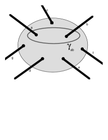
Figure 7: The $\hat{T}_{ab}$ operator. The shaded region is the punctured boundary ${\cal S}^{2}-\{{\alpha}\}$.

But if, as we have argued, the punctures correspond to $D0$ branes, then, for an appropriate choice of $G_{q}$, this matrix of operators should correspond to the matrix description of the dynamics of $D0$ branes, hypothesized by Banks, Fischler, Shenker and Susskind. In that description there is a matrix of operators $\hat{X}^{i}_{ab}$ for every transverse coordinate $i$ in light cone coordinates of flat $11$ dimensional Minkowski spacetime.

We will first establish a correspondence for any odd dimension $D$. For a $D$ dimensional matrix model we have a matrix of coordinates $\hat{X}_{ab}^{i}$, with $i=1,\ldots,D$. To establish a correspondence we have to first choose the algebra $G_{q}$ appropriately and then find out where this transverse coordinate $i$ lives. As there is no background manifold there is no transverse space, this has to emerge in the appropriate continuum limit.

In odd dimension $D$ we can represent the bosonic matrix model by choosing $G_{q}=Spin(D)$. We will take traces of holonomies in a spinor representation of $Spin(D)$ in which there are $D$ gamma matrices $\Gamma^{i}$. We may then define the classical phase space functions,

$$T^{i}[\gamma]=Tr\left[\Gamma^{i}e^{\int_{\gamma}A}\right]$$ (16)

From (16) we have a matrix of quantities given by

$$T^{i}_{ab}=Tr\left[\Gamma^{i}e^{\int_{\gamma_{ab}}A}\right]$$ (17)

We make several comments on these variables. First, note that the diagonal elements use $\gamma_{ab}=\gamma_{aa}$, the curve that wraps twice around the single puncture.

Second, note that as in the matrix model, we can consider the $N$ eigenvalues $r^{i}_{a}$ of the $D$, $N\times N$ matrixes $T^{i}_{ab}$. These give us $N$ points in $R^{D}$. In the limit $N\rightarrow\infty$ the usual arguments from the original matrix mode[21, 22] may be used to define a mapping from an $S^{2}$ into $R^{D}$. Thus, in this limit we see emerge a description of a membrane moving in $R^{D}$.

However there are some differences with the usual matrix model. First, there are constraints coming from the conditions that the trace of the holonomy around single punctures are fixed. The effect of these will depend on the dimension. Then we must notice that the $T^{i}_{ab}$ are not a commuting set, instead $\{T^{i}_{ab},T^{j}_{cd}\}\approx 1/k$ whenever $a$ or $b$ is equal to $c$ or $d$. Thus the quantities (17) cannot correspond directly to the coordinates of a matrix model. However, recall that in $2+1$ and $3+1$ dimensions the cosmological contant is inversely proportional to a power of $k$, so that $\Lambda\rightarrow 0$ when $k\rightarrow\infty$ (see (2). This suggests that we should seek to recover the standard matrix model, which corresponds to supergravity in $11D$ with vanishing cosmological constant, in the limit $k\rightarrow\infty$. We will then need to rescale the fields so as to recover the matrix model in the limit $k\rightarrow\infty$.

Finally, we must also note that the quantities (17) are not gauge invariant. They are non-vanishing when evaluated on the classical phase space, which is the flat connections on the punctured surface. If we turn them into operators in the space of intertwiners they will vanish, because only gauge invariant quantities are non-vanishing. This is because we are constructing the theory in terms of gauge invariant quantities; and any particular coordinates on a background manifold which emerges from this description will be gauge non-invariant. For this reason we will proceed to first construct formal operators that represent pieces of gauge invariant quantities, which include the $T^{i}[\gamma]$. We then combine these to form gauge invariant operators.

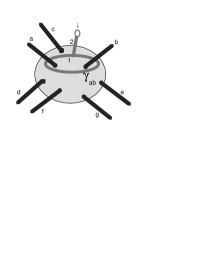
Figure 8: The $\hat{T}_{ab}^{i}$ operator. The $i$ in the circle stands in the classical theory for the trace of the phase space observable against $\Gamma^{i}$. In the quantum theory it stands for a formal operator in which the $i$ is contracted against another open $2$ line that acts somewhere else in the state.

One of the gauge invariant quanties we can construct is closely related to the hamiltonian of the $D$ dimensional matrix model. To do this first find a set of momentum functionals $P_{i}^{ab}$ so that,

$$\{T^{i}_{ab},P^{cd}_{j}\}=\delta^{i}_{j}\delta^{c}_{a}\delta^{d}_{b}$$ (18)

These must exist, but we will not construct them explicitly, instead, the appropriate quantum operators will be constructed below. We may then construct a classical hamiltonian that matches that of the bosonic sector of the matrix model, in the limit $k\rightarrow\infty$ in which the $T^{i}_{ab}$’s become commuting variables.

$$H={g^{2}\over 2}Tr\left[P_{i}P_{i}\right]+{1\over g^{2}}Tr\left([T^{i},T^{j}],[T_{i},T_{j}]\right)$$ (19)

where $g$ is a dimensionless coupling constant.

What this means is that a system which is closely related to the matrix model may be coded in the classical phase space of the boundary observables. However, this is only a step, for in the present theory the dynamics has already been given by the substitution moves in the bulk. The dynamics of the punctures will then be induced by the bulk-to-boundary map, applied as discussed in section 3. What we then want to know is whether the bulk evolution moves can be chosen so that the dynamics of the matrix model is induced as an effective quantum dynamics of the punctures. To do this we will proceed in two steps. First, we construct a quantum hamiltonian, $\hat{H}$, on the boundary, state space ${\cal V}_{j_{a}}^{S^{2}}$ which yields (19) to leading order. Second, we will find a set of substitution moves and amplitudes which reproduce the quantum dynamics generated by $\hat{H}$.

We will carry this out first for the bosonic matrix models in $D=3$, then we extend the correspondence, in turn to the supersymmetric matrix model in $D=3$ the bosonic matrix model in $D=9$, and, finally, a supersymmetric matrix model in $D=9$ that reduces in a certain limit to the dWHN-BFSS model.

7 The $D=3$ matrix model

We first study the bosonic matrix model in $D=3$ in which case we take $G_{q}=SU_{q}(2)$.

We begin by asking how the classical limit should emerge. As the punctures must correspond, in the reduction to quantum general relativity, to quanta of area, the continuum limit must be the limit of large area, in Planck units. In the cases associated with general relativity or supergravity in $3+1$ dimensions,in which $G=SU(2)$ or $Osp(1|2)$,it is known that the area of a surface with $N$ punctures with labels $j_{\alpha}$ is proportional to $\sum_{\alpha}\sqrt{C(j_{\alpha})}$ where $C(j_{\alpha})$ is the quadratic casimer operator. Furthermore, as shown in [16] the most probable way of reaching the limit of large area, in which the Bekenstein bound is saturated, is the one in which each puncture carries a minimum area, corresponding to the smallest representation, $j_{1/2}$ of $G_{q}$. In this case the dimension of the boundary state space saturates the Bekenstein bound as the area is taken to infinity. This tells us that we should expect the continuum limit to emerge in the case that all the punctures have the same value $j_{\alpha}=j_{1/2}$. For these, most probably states, the limit of large area is $N\rightarrow\infty$, where $N$ is the number of punctures.

7.1 Matrix valued operators on ${\cal V}^{{\cal S}^{2}}_{j_{\alpha}}$.

In the case of $D=3$, the the diagonal elements $T_{aa}^{i}\equiv v^{i}$ are fixed by the condition that the Wilson loops around single punctures are fixed in terms of $k$ and the representation label. Physically, this means that the vectors $v^{i}_{a}$ live in $S^{2}$. This is reminiscent of the spin geometry theorem, which was the motivation for the original introduction of the spin network formalism by Penrose in the early 1960’s[37]. There a map is found between $SU(2)$ spin networks with $N$ ends, labeled by spins $j_{\alpha}$ and $N$ points on a two sphere. This is gotten by constructing an operator $\hat{X}_{ab}$ which connects the $a$’th to the $b$’th external edge with a spin $1$ line. If $|\Gamma>$ is an ordinary $SU(2)$ spin network, with $N$ ends, then the map $\Phi$ produces in this case an $SU(2)$ intertwiner $|\tilde{\Gamma}>$. Since $\hat{X}_{ab}$ acts adjacent to the ends, its action on intertwiners $|\tilde{\Gamma}>$ is well defined. Penrose then finds that the expectation values,

$$Y_{ab}\equiv{<\tilde{\Gamma}|\hat{X}_{ab}|\tilde{\Gamma}>\over<\tilde{\Gamma}|\tilde{\Gamma}>}=\cos(\theta_{ab})$$ (20)

for $a\neq b$ define $N(N-1)/2$ angles $\theta_{ab}$ which, in the case that they do not vanish, may be interpreted consistently to give relative angles between $N$ points in a two sphere[37]. This is called the spin-geometry theorem.

In fact, it is easy to show that for $G=SU(2)_{q}$,

$$\hat{T}_{ab}={16\pi^{2}j_{a}j_{b}\over k^{2}}\hat{X}_{ab}$$ (21)

Thus, the $G=SU(2)$ case of the construction of the previous section is closely related to Penrose’s spin geometry theorem. This correspondence suggests the following construction, which we will shortly extend to general $G_{q}$. We introduce a set of formal operators $\hat{S}^{i}_{ab}$ that act on the bulk state space, ${\cal H}^{N}_{j_{a}}$. Given a state $|\Gamma,j_{a},\mu_{i}>\in{\cal H}^{N}_{j_{a}}$, these act as follows. (See Figure (9).)

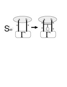
Figure 9: The definition of the operator $\hat{S}^{i}_{ab}$ in the $D=3$ cases. The added trinions are in grey, all the labels are in the adjoint representation. The remainder of the surface is indicated by $\Gamma$, other ends on the boundary are not shown.

We break the tube going to the puncture $a$ along a circle $c_{a}$ with label $j_{a}$. We then insert a new trinion as follows. Two of the three punctures of the trinion join the two sides separated at $c_{a}$, with identical labels $j_{a}$. The third we label with the adjoint representation $Adj$ of $G_{q}$ and leave open for the moment. We then do the same with the puncture $b$. We then introduce a third trinion one puncture of which is tied to the free puncture of the new trinion inserted adjacent to $a$. A second puncture is joined to the free puncture adjacent to $b$. Each of these have labels $Adj$. At the third puncture, we introduce an operator that corresponds to tracing over the gamma matrix $\Gamma^{i}$. This is a formal operation, it means that this operator stands for a family of operators where the $i$ index is contracted with another $i$ index, with a tube labeled by $Adj$. We call the resulting formal operator $\hat{S}_{ab}^{i}$.

This then induces an operator in ${\cal V}_{j_{a}}^{S^{2}}$, which we call $\tilde{S}_{ab}^{i}$, defined with the help of the holographic map (7). Given $|\Psi>\in{\cal V}_{j_{a}}^{S^{2}}$ let $|\Psi^{\&}>$ be any state in ${\cal H}^{N}_{j_{a}}$ such that

$$\Phi\circ|\Psi^{\&}>=|\Psi>$$ (22)

This is non-unique but it doesn’t matter, because we are about to act only on the edges that are adjacent to the punctures, and these are fixed. Then we define the action of $\tilde{S}_{ab}^{i}$ on $|\Psi>$ by

$$\tilde{S}_{ab}^{i}\circ|\Psi>\equiv\Phi\circ{S}_{ab}^{i}\circ|\Psi^{\&}>.$$ (23)

It is also straightforward to show that $\tilde{S}_{ab}^{i}$ is related to $T^{i}_{ab}$ in the $SU(2)_{1}$ case by

$$T^{i}_{ab}={16\pi^{2}j_{a}j_{b}\over k^{2}}\tilde{S}^{i}_{ab}$$ (24)

The spin geometry theorem then gives us some insight into the meaning of the off diagonal elements of the $T_{ab}$ and $T_{ab}^{i}$ at least for $D=3$. When treated as classical phase space variables, the combination

$$Y_{ab}^{AB}=\epsilon^{AB}T_{ab}+\imath\tau^{AB}_{i}T^{i}_{ab}$$ (25)

may be interpreted as an $SU(2)$ element that rotates the point $v^{i}_{a}$ into the point $v^{i}_{b}$ on the $S^{2}$. One can see from this that the off diagonal elements of $T^{i}_{ab}$ are proportional to the $\sin(\theta_{ab})$, thus they measure the distance on the $S^{2}$ between the the points $v^{i}_{a}$ and $v^{i}_{b}$.

However, we may also note from the definition of the operators (16) and (23) that the $ab$ elements of $<\Gamma|T^{i}_{ab}|\Gamma>$ will vanish when the edges $a$ and $b$ come from disconnected pieces of the spin network $|\Gamma>$. (As this is a formal operator it means it vanishes when the index $i$ is contracted against any operator.) This means that the off diagonal elements vanish when the ends corresponding to the points fall into disconnected clusters, corresponding to $\Gamma$ having disconnected pieces.

Thus, a potential of the form of that in (19) is minimized either by the points lying on top of each other, or falling into disconnected clusters.

7.2 Construction of the quantum matrix model Hamiltonian on the space of intertwiners

We now are ready to express the matrix model dynamics, given classically by (19), in terms of operators on ${\cal V}_{j_{a}}^{S^{2}}$. Care must be taken as $\hat{S}^{i}_{ab}$ differs from $T^{i}_{ab}$ by powers of $k$ and $k$ is taken to infinity in the limit that defines the vanishing of the cosmological constant and hence the limit in which the matrix model is recovered. We know that it is the $T^{i}_{ab}$’s that must be the basic operators that define the matrix model, as it is these that go into the commuting coordinates of the matrix theory in the limit that $k\rightarrow\infty$. But when computing it is easier to work with the $\tilde{S}_{ab}^{i}$ as they have a simple action on states.

We may use (24) to write a quantization of the potential energy term of classical matrix model hamiltonian, (19), as an operator on ${\cal V}_{j_{a}}^{S^{2}}$

$$\hat{V}={1\over g^{2}}\left({2\pi\over k}\right)^{8}Tr\left([\tilde{S}^{i},\tilde{S}^{j}][\tilde{S}_{i},\tilde{S}_{j}]\right).$$ (26)

To define the kinetic energy term we need to define the conjugate momentum operator, $\tilde{\pi}^{ab}_{i}$ such that

$$\{\tilde{S}_{ab}^{i},\tilde{\pi}^{cd}_{j}\}=\delta^{i}_{j}\delta^{c}_{a}\delta^{d}_{b}$$ (27)

This is defined diagramatically below in Figure (12). We may then write the hamiltonian corresponding to the matrix model.

$$\tilde{H}={g^{2}k^{4}\over 32\pi^{2}}Tr\left[\tilde{\pi}^{i}\tilde{\pi}^{i}\right]+{1\over g^{2}}\left({2\pi\over k}\right)^{8}Tr\left([\tilde{S}^{i},\tilde{S}^{j}][\tilde{S}_{i},\tilde{S}_{j}]\right).$$ (28)

Here we have used the fact that all the punctures are taken in the fundamental representation $j=1/2$, which is necessary to have the largest entropy per area of the holographic surface.

7.3 Realizing the $D=3$ Matrix theory hamiltonian in terms of local evolution moves

We now proceed to show that there is a choice of the fundamental dynamics that reproduce the Hamiltonian of the $D=3$ matrix model acting on the boundary state space ${\cal V}_{j_{a}}^{S^{2}}$. The potential energy term in (28), is formally given by,

$$\hat{V}=Tr\left([\tilde{S}^{i},\tilde{S}^{j}][\tilde{S}_{i},\tilde{S}_{j}]\right)$$ (29)

We may note that the $\tilde{S}_{ab}^{i}$ operators, like the $\hat{T}_{ab}^{i}$ do not have exactly the same commutation relations as those of the dWHN-BFSS model. Rather we have $[\tilde{S}_{ab}^{i},\tilde{S}_{bc}^{i}]\neq 0$, as can be easily checked explicitly. Thus, it is necessary to choose an operator ordering when realizing (29) as an operator. We make the simplest choice of symmetric ordering, which is shown in Fig. (11).

Figure 10: The action of the potential energy term, $Tr\left([\tilde{S}^{i},\tilde{S}^{j}][\tilde{S}_{i},\tilde{S}_{j}]\right)$ of the $D=3$ matrix model on the boundary. The action of the operator is to add the shaded figure. In this and the following figures, unmarked wide shaded lines are in the adjoint representation.

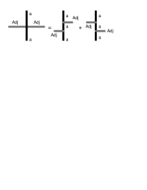
Figure 11: The definition of symmetric ordering used in the definition of the potential energy operator shown in Fig. (10).

We can then form the potential energy operator (29) by acting four times as indicated. The result is indicated in Figure (10), it is an operator that sums over all $4$-tuples of edges $a,b,c,d$ and adds adjacent to the punctures the graph indicated there. The figure added may be visualized as an $H$, with the external edges labeled by $Adj$’s going to the four edges immediately adjacent to the nodes $a,b,c,d$ and the cross-piece labeled by an $i\in Adj\times Adj$, which is summed over. The latter is the result of the antisymmetrization in (29). Finally, the overall weight is

$${1\over g^{2}}w(i)$$ (30)

where in standard notation [45]

$$w(i)={\Delta_{i}\over\Theta(2,i,2)}\left(1-\lambda^{22}_{i}\right)$$ (31)

The next step is to invent the momentum operators $\tilde{\Pi}_{i}^{ab}$ which are to be conjugate to the $\tilde{S}_{ab}^{i}$. We chose them so that, on ${\cal V}_{j_{a}}^{S^{2}}$

$$[\tilde{S}_{ab}^{i},\tilde{\Pi}_{j}^{cd}]=i\hbar\delta^{i}_{j}\delta^{c}_{a}\delta^{b}_{d}$$ (32)

$\tilde{\Pi}_{j}^{cd}$ can then be defined on a basis of states in ${\cal V}_{j_{a}}^{S^{2}}$ given by intertwiners of $G_{q}$, decomposed so that there are two framed edge of spin $r$ and $s$ linking the edges that go to $c$ and $d$ to a trinion, which has a third edge of spin $u$ going outward(See Figure (12).) For every $c$ and $d$ such a basis can be constructed. The action of $\tilde{\Pi}_{j}^{cd}$ on this state is to remove the component where $r=s=u=Adj$ and replace it with the state in which the now opened edge $u$ is traced with $\gamma^{i}$.

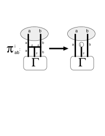
Figure 12: The action of the momentum operator $\tilde{\Pi}_{i}^{ab}$. $2$ denotes the adjoint representation.

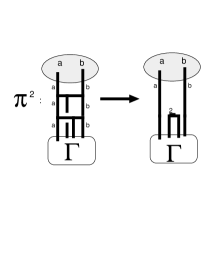
Figure 13: The action of the kinetic energy term, $Tr\left(\tilde{\Pi}_{i}\tilde{\Pi}_{i}\right)$ of the $D=3$ matrix model on the boundary.

We then compute the square of $\tilde{\Pi}_{i}^{ab}$. The action $\sum_{i}\tilde{\Pi}_{i}^{ab}\tilde{\Pi}_{i}^{ab}$ in the basis described is indicated in Figure (13).

By adding the kinetic and potential energy together with the weights given by (28), we have the matrix Hamiltonian for the evolution of the state in ${\cal V}_{j_{a}}^{S^{2}}$,

$$\hat{H}={g^{2}k^{4}\over 32\pi^{2}}Tr\left(\tilde{\Pi}_{i}\tilde{\Pi}_{i}\right)+{1\over g^{2}}\left({2\pi\over k}\right)^{8}Tr\left([\tilde{S}^{i},\tilde{S}^{j}][\tilde{S}_{i},\tilde{S}_{j}]\right)$$ (33)

We can then form the evolution operator on ${\cal V}_{j_{a}}^{S^{2}}$ as

$$\hat{U}(s,t)=e^{i(t-s)\hat{H}}.$$ (34)

With this hamiltonian in hand, we are prepared to ask whether there is a choice of evolution move and amplitude that reproduces its effect in appropriate circumstances. Let us begin with the simplest possible circumstance, which is where the holographic surface bounds a small region, containing only the parts of the surfaces ${\cal S}^{g}$ on which the replacement operator acts. In this case the map $\Phi$ is trivial, and we can in the right limits, establish an exact correspondence between the replacement moves and their amplitudes and the hamiltonian (33).

It is harder to establish the correspondence for evolution moves that act far from the holographic surface, and this has not yet been done. It is likely that this will be where supersymmetry plays a crucial role, to enforce a non-perturbative version of a non-renormalization theorem, that will imply that one can move the evolution move from close to the boundary to deep inside the bulk without changing the form of the Hamiltonian that describes the dynamics induced on the punctures in the boundary.

For the present we restrict ourselves to the simplest case, which is where the bulk contains the simplest possible states on which the different terms of the matrix model hamiltonian may act. Because of the existence of the free coupling constant $g$, the case where the evolution move acts just inside the holographic surface is sufficient to pick out a set of evolution moves that match for both large and small $g$.

We are looking for a replacement move ${\cal R}_{matrix}$ of the form discussed in section 5 and an operator $\hat{h}$ in the space ${\cal V}_{j_{a}}^{S^{2}}$ that bounds the region where the replacement occurs. In the simplest case, we may identify that surface with the holographic surface on which the hamiltonian (33) acts.

We will consider first the limit $g^{2}\rightarrow 0$ and then the limit $g^{2}\rightarrow\infty$.

In the first case we are interested to match the potential energy in (33) to a single action of a replacement move. The simplest case to study is that where $N=4$. We take the initial state in ${\cal H}^{4}_{j_{a}}$ to be the simplest possible one, indicated in Figure (10) in which the four edges are tied together by a four punctured sphere. This state is labeled by an intertwiner on the four punctured sphere, which we may indicate simply as $|\mu>$. In this case the map (7) commutes with the action of $\hat{H}$ because the region cut out by the evolution move is the whole interior. The effect of the evolution move may be arrived at by simply lifting the effect of $\hat{H}$ from ${\cal V}_{j_{a}}^{S^{2}}$ to ${\cal H}^{N}_{j_{a}}$. The kinetic energy term does not act, while the potential energy term (29) increases the genus by $\Delta g=8$, as shown in Figure (14). If the final state after the replacement move is indicated by $|Final>$ then in this case the amplitude is given by

$${\cal A}[\mbox{Figure (\ref{[][]bulkfig}) }]=<\tilde{Final}|e^{\imath\hat{H}}|\tilde{\mu}>\approx{i\over g^{2}}\left({2\pi\over k}\right)^{8}<\tilde{Final}|\hat{V}|\tilde{\mu}>$$ (35)

Here we have taken the time interval to be one because the initial state has been completely replaced in the interior, corresponding to one time step in any slicing.

Figure 14: The replacement move, $R_{V}$, in the bulk that induces the potential energy term, $Tr\left([\tilde{S}^{i},\tilde{S}^{j}][\tilde{S}_{i},\tilde{S}_{j}]\right)$ of the matrix model on the boundary in the simplest case.

To see the effects of the kinetic energy dominate we consider instead the limit where $g^{2}$ is large, in which case the leading order term is its action on states in ${\cal H}^{N}_{j_{a}}$ where the interior surface has genus $4$. The action is shown in Figure (15). The change in genus is $\Delta g=-3$. Indicating the initial and final states in ${\cal H}^{4}_{j_{a}}$ by $|in>$ and $|out>$ the amplitude is

$${\cal A}[\mbox{Figure (\ref{bulkpi2fig})}]=<\tilde{future}|e^{i\hat{H}}|\tilde{past}>\approx{ig^{2}k^{4}\over 32\pi^{2}}<\tilde{future}|Tr\left(\tilde{\Pi}_{i}^{ab}\tilde{\Pi}_{i}^{ab}\right)|\tilde{past}>$$ (36)

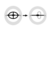
Figure 15: The replacement move, $R_{K}$, in the bulk that induces the kinetic energy term, $Tr\left(\tilde{\Pi}_{i}\tilde{\Pi}_{i}\right)$ in the simplest case in which it acts.

The replacement operator $\cal R$ must reduce to these two limits. The simplest choice that does this is to take the sum of two operators

$${\cal R}={\cal R}_{K}+{\cal R}_{V}$$ (37)

To summarize, the first of these moves is a genus $\Delta g=-3$ move shown in Figure (15). The amplitude for it is given by

$${\cal A}[{\cal R}_{K}]={ig^{2}k^{4}\over 32\pi^{2}}<\tilde{future}|Tr\left(\tilde{\Pi}_{i}^{ab}\tilde{\Pi}_{i}^{ab}\right)|\tilde{past}>$$ (38)

The second move is the genus $\Delta g=+8$ indicated in Figure (14), to which we assign an amplitude

$${\cal A}[{\cal R}_{V}]={i\over g^{2}}\left({2\pi\over k}\right)^{8}<\tilde{future}|\hat{V}|\tilde{past}>$$ (39)

These choices complete the definition of the theory for the case $G_{q}=SU(2)_{q}$.

8 Extension to $Osp(1|2)$

We now extend the matrix model to include fermions, keeping for this section still to the $D=3$ case. This can be done by extending the algebra to $G_{q}=Osp(1|2)$. It is easy to see that the two moves ${\cal R}_{1}$ and ${\cal R}_{2}$ we have just defined correspond to the bosonic part of the $D=3$ matrix model Hamiltonian. The only adjustment that needs to be made is that the spin $1$ and spin $1/2$ edges are replaced, respectively, by the adjoint and fundamental representations of $Osp(1|2)$.

We must then add a third replacement move to correspond to the fermionic term in the matrix model. As we did with the bosonic part we first construct the hamiltonian on the boundary state space, ${\cal V}_{j_{a}}^{S^{2}}$, and then pick an evolution move and amplitude that reproduces it.

The algebra $Osp(1|2)$ has five generators, which are the three angular momenta, $J^{ij}$ and the supersymmetry generators $\hat{Q}^{A}$, where $A=1,2$. The algebra includes,

$$[J^{ij},Q^{A}]=\sigma^{ij\ A}_{\ \ B}Q^{B}$$ (40)

where $J^{ij}$ are the generators of $Spin(3)$ and $\sigma^{ij\ A}_{B}$ are its usual representation via Pauli matrices. The fundamental representation of $Osp(1|2)$ is three dimensional, and comprises the spin $0$ and $1/2$ representations of $SU(2)$. We write its components as $\bar{A}=(0,1,2)=(0,A)$. The adjoint representation is generated by the graded symmetric generators $J^{(\bar{A}\bar{B})}$, where

$$J^{(\bar{A}\bar{B})}={1\over 2}\left[J^{\bar{A}\bar{B}}+(-1)^{g(\bar{A})g(\bar{B})}J^{\bar{B}\bar{A}}\right]$$ (41)

where $g(0)=1,g(A)=0$. The embedding of the generators in the fundamental representation is

$$\Gamma^{\bar{A}\bar{B}}=\left(\begin{array}[]{cc}\sigma^{AB}&Q^{B}\\ Q^{A}&0\end{array}\right)$$ (42)

Thus, $\sigma^{A}_{B}$ is imbedded in the $2\times 2$ block $\bar{A},\bar{B}=A,B$ of $\Gamma^{\bar{A}\bar{B}}$ and $[Q^{A}]_{\bar{A}}^{\bar{B}}$ is represented by $[Q^{A}]_{B}^{0}=[Q^{A}]_{0}^{B}=\delta_{B}^{A}$ and $[Q^{A}]_{0}^{0}=0$.

We may construct the superconnection one-form

$${\cal A}^{\bar{A}}_{\bar{B}}=A^{AB}\sigma^{AB\ \ \bar{B}}_{\ \bar{A}}+\lambda^{D}Q_{D\ \ \bar{B}}^{\ \bar{A}}.$$ (43)

The phase space of the boundary theory is then given by the flat superconnections on the punctured $S^{2}$ representing the boundary. We then define the supersymmetric extensions of the $D0$ brane coordinates on the phase space of the boundary theory to be

$$\hat{T}^{AB}_{ab}=Tr\left(\sigma^{AB}e^{\int_{\gamma_{ab}}{\cal A}}\right)$$ (44)

$$\hat{T}^{A}_{ab}=Tr\left(Q^{A}e^{\int_{\gamma_{ab}}{\cal A}}\right)$$ (45)

Quantum operators corresponding to these may be constructed as we did in the last section, using instead of $Spin(3)$ the fusion algebra of $Osp(1|2)_{q}$.

The Hamiltonian is constructed from two sets of operators, corresponding to the fundamental and the adjoint representation, respectively. To see how these correspond to the usual coordinates of the matrix model we write the adjoint rep. operators as

$$S^{\bar{A}\bar{B}}_{ab}=S^{\bar{B}\bar{A}}_{ab}=\left(\begin{array}[]{cc}S^{AB}_{ab}&\lambda^{B}_{ab}\\ \lambda^{A}_{ab}&0\end{array}\right)$$ (46)

and the fundamental representation fields as

$$\Psi^{\bar{A}}_{ab}=\left(\begin{array}[]{c}\psi^{A}_{ab}\\ \phi_{ab}\end{array}\right)$$ (47)

We see that we have auxillary fields $\phi_{ab}$ and $\lambda^{A}_{ab}$ which are, in terms of $SU(2)$ reperesentations, a matrix-valued scalar and spinor.

Conjugate to $S^{\bar{A}\bar{B}}_{ab}$ we have canonical momenta $\Pi^{\bar{A}\bar{B}}_{ab}$, satisfying

$$\{S^{\bar{A}\bar{B}}_{ab},\Pi_{\bar{C}\bar{D}}^{cd}\}=\delta^{(\bar{A}\bar{B})}_{\bar{C}\bar{D}}\delta^{c}_{a}\delta^{d}_{b}$$ (48)

while the fermions satisfy

$$\{\Psi^{\bar{A}}_{ab},\Psi_{\bar{B}}^{cd}\}_{+}=\delta^{\bar{A}}_{\bar{B}}\delta^{c}_{a}\delta^{d}_{b}$$ (49)

In terms of these $Osp(1|2)$ representations the supersymmetric $D=3$ matrix model is

$$H^{susy,D=3}={g^{2}\over 2}Tr\left[\Pi^{\bar{A}\bar{B}}\Pi_{\bar{A}\bar{B}}\right]+{1\over g^{2}}Tr\left([S^{\bar{A}\bar{B}},S^{\bar{C}\bar{D}}][S_{\bar{A}\bar{B}},S_{\bar{C}\bar{D}}]\right)+Tr\left(\bar{\Psi}_{\bar{A}}\left[\tilde{S}^{\bar{A}\bar{B}},{\Psi}_{\bar{B}}\right]\right)$$ (50)

If one expands it is not difficult to see that the auxilary fields $\phi_{ab}$ and $\lambda^{A}_{ab}$ decouple, leading to the $N=1$, $D=3$ matrix model,

$$H^{susy,D=3}={g^{2}\over 2}Tr\left[\Pi^{i}\Pi_{i}\right]+{1\over g^{2}}Tr\left([S^{i},S^{j}][S_{i},S_{j}]\right)+Tr\left(\bar{\Psi}_{A}\sigma_{i}^{AB}\left[\tilde{S}^{i},\tilde{\Psi}_{B}\right]\right)$$ (51)

We then proceed as before to represent these as operators in the space of intertwinors for the quantum deformation of $Osp(1|2)$, which may be constructed as the space of states of the $Osp(1|2)$ Chern-Simons theory corresponding to the flat superconnections on the punctured surface. The operators that corresponds to $S^{\bar{A}\bar{B}}_{ab}$ and its momenta $\Psi^{\bar{A}}_{ab}$ are exactly those shown in Figures (9) and (12) where the adjoint representation of $Osp(1|2)$ is now used. For the fermionic variables we use the operator shown in Figure (16)

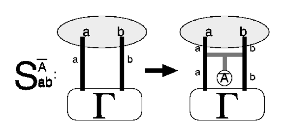
Figure 16: The action of the fermionic operator corresponding to the fundamental representation of $Osp(1|2)$. Note that the intertwinor shown is allowed in the representation theory of $Osp(1|2)$ as the condition that the spins must add up to be even is not satisfied[68].

The fermionic part of the matrix model hamiltonian is then expressed as an operator on ${\cal V}_{j_{a}}^{S^{2}}$ by translating the expression

$$H^{f}={4\pi^{2}\over k^{2}}Tr\left(\bar{\Psi}_{\bar{A}}\left[\tilde{S}^{\bar{A}\bar{B}},\tilde{\Psi}_{\bar{B}}\right]\right)$$ (52)

into the action shown in Figure (17).

Figure 17: One of two terms of the fermionic term of the matrix model, (52). This is the simplest state in which it can act. In the $D=3$ theory grey tubes are in the $3$-dimensional fundamental representation of $Osp(1|2)$ and thicker grey tubes are in the $5$-dimensional adjoint representation. In the other term the order of the two thick grey tubes is reversed.

The fermionic momentum variable $\tilde{\Pi}_{\bar{A}}=\bar{\Psi}_{\bar{A}}$ is constructed by following the same procedure we used for the bosonic momenta. It yields the operator shown in Figure (18).

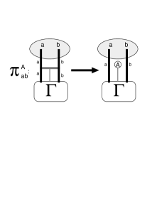
Figure 18: The action of the fermionic momentum operator.

We then find a replacement operator which in the simplest case reproduces (52). The change of genus in this case is $\Delta g=+1$. It is given in Figure (19). The corresponding amplitude is given by,

$${\cal A}[(\mbox{Figure }\ref{Hfbulkfig})]=i<\tilde{future}|H^{f}|\tilde{past}>$$ (53)

Figure 19: The replacement move in the bulk that induces the fermionic term of the matrix model, (52).

The full replacement operator for $G_{q}=Osp(1|2)$ is then given by the $Osp(1|2)$ replacement operators

$${\cal R}={\cal R}_{K}+{\cal R}_{V}+{\cal R}_{f}$$ (54)

9 The bosonic matrix model in $D=9$

The procedure we have just used in $D=3$ can be used to construct a background indepedent membrane theory associated with a matrix model in any dimension $D$. The basic idea in each case is that the matrix coordinates are given by operators defined like the $S_{ab}^{i}$ in the space of intertwiners of the punctured sphere for some group $G_{q}$. In the bosonic case $G_{q}$ will generally be the quantum deformation of $SO(D)$ gotten by quantizing Chern-Simons theory on a three manifold which is the punctured sphere cross the interval. In the supersymmetric case the construction may be considerably more complicated, as we saw in the $D=3$ case, where auxiliary fields entered the construction. In this case they decoupled but this is not gauranteed to happen in the general case.

We now briefly sketch the $D=9$ case which is appropriate for the dWHN-BFSS matrix model. Full details will appear elsewhere[71].

It is straightforward to extend the definition of the $D=3$ bosonic matrix model to a bosonic matrix model in $9$ dimensions, by choosing for $G_{q}$ the quantum deformation of $SO_{q}(9)$. The classical phase space of the holographic observables will be given by the conformal blocks constructed from the quantization of a $Spin(9)$ Chern-Simons theory. The classical matrix model coordinates will be given by (17) with the traces and the $\Gamma^{i}$ taken in the $16$ dimensional spinor representation of $SO(9)$, which we denote by $\Delta$. The corresponding quantum operators $S^{i}_{ab}$ is shown in Fig. (20), it is similar to the $D=3$ case, but a bit more complicated. The reason is that the calculation of the quantum operator involves the decomposition of the product of spinor representations, and above $D=3$ this includes more than the adjoint and a scalar. In $D=9$ we have, $\Delta\otimes\Delta=C\oplus V\oplus V^{2}\oplus V^{3}\oplus V^{4}$ where $V=R^{9}$ and $V^{p}$ stands for the $p$-fold antisymmetric product. With the trace part proportional to $C$ removed, this replaces the adjoint representation when we extend from the $SU(2)$ case to the $Spin(9)$ case.

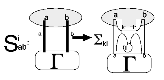
Figure 20: The definition of the operator $\hat{S}^{i}_{ab}$ in the $D=9$ case. The sums are $k,l=V\oplus V^{2}\oplus V^{3}\oplus V^{4}=\Delta\otimes\Delta-C$. The $i$ stands for the projection of the vector representation $V$. The remainder of the surface is indicated by $\Gamma$, other ends on the boundary are not shown.

The momentum operator is defined in Fig. (21), which works just as in the $D=3$ case.

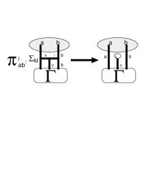
Figure 21: The action of the momentum operator in the $D=9$ case. $\tilde{\Pi}_{i}^{ab}$.

The potential energy and kinetic energy terms are modified appropriately, so that the adjoint representation of $SU(2)$ is everywhere replaced by the sum over the decomposition of $\Delta\otimes\Delta-C$. The matrix model hamiltonian is then represented in ${\cal V}^{{\cal S}^{2}}_{j_{\alpha}}$ by the hamiltonian (33) and the simplest operator in the bulk which induces it is again given by the two replacement operators ${\cal R}_{K}$ and ${\cal R}_{V}$ as in (37), where in each case the adjoint representation is replaced by the tracefree sum $\Delta\otimes\Delta-C$.

10 The supersymmetric extension in $D=9$

What remains to arrive at a theory that includes the full dWHN-BFSS matrix model is then only to include the fermionic degrees of freedom. To do this one must pick an appropriate superalgebra $G_{q}$ so that one can write a superconnection of the form (43) corresponding to the supersymmetric extension of the matrix model. The spinor representation of $SO(9)$ is $16$ dimensional, to incorporate one spinor degree of freedom what is required is a superalgebra with a $17$ dimensional fundamental representation whose bosonic subalgebra has a $Spin(9)$ subalgebra.

There are several choices for $G_{q}$ which each give rise to a theory whose degrees of freedom include those of the dWHN-BFSS matrix model. One of the simplest, which involves only one fermionic matrix variable, is $SU(16|1)$. Given that the norm in the spinor representation of $Spin(9)$ is symmetric we have the inclusions, $Spin(9)\subset SO(16)\subset SU(16)$. This has a fundamental $17$ dimensional representation, which is the smallest supermultiplet of $Spin(9)$ comprising the scalar and the spinor. This is the analogue of the $3$ dimensional representation of $Osp(1|2)$ used in the supersymmetric $D=3$ matrix model and in supersymmetric spin networks in $D=3+1$[68].

A consequence of the unification in a larger group, however is the inclusion of additional bosonic degrees of freedom. This is seen by the fact that the symmetric product of spinor representations of $Spin(9)$ involves

$$16\otimes_{sym}16=R\oplus V\oplus V^{4}=1\oplus 9\oplus 126$$ (55)

The $126$ is the four index antisymmetric tensor in $D=9$. In terms of indices this corresponds to

$$S^{A}\otimes_{sym}S^{B}=\delta^{AB}\phi\oplus\Gamma^{AB}_{i}V^{i}\oplus\Gamma^{AB}_{ijkl}V^{ijkl}$$ (56)

where $\Gamma^{AB}_{abcd}$ is the antisymmetric product of $9$ dimensional Gamma matrices $\Gamma^{AB}_{a}$. This means that the matrix model degrees of freedom have been extended from $X^{i}_{ab}$ to $X^{(AB)}_{ab}$, so as to include naturally the four (or, by duality, five) index antisymmetric tensor fields and a scalar:

$$X^{(AB)}_{ab}=\delta^{AB}S_{ab}+\Gamma^{AB}_{i}X^{i}_{ab}+\Gamma^{AB}_{ijkl}V^{ijkl}_{ab}$$ (57)

The resulting theory involves then the addition of central charges to the $D=9$ superalgebra,

$$\{Q^{A},Q^{B}\}=\delta^{AB}+H\Gamma^{AB}_{i}P^{i}+\Gamma^{AB}_{ijkl}Z^{ijkl}$$ (58)

This is, of course, not surprising as the usual matrix model superalgebra closes on shell, and we are working in a formalism in which the supersymmetry should be manifest. It is possible that these additional degrees of freedom provide an alternative way for the transverse five-brane to be represented in the matrix model; this will be discussed elsewhere[71].

One can then define the theory in terms of the same three replacement moves as the $Osp(1|2)$ case, indicated in (54), with the appropriate replacements of $Osp(1|2)$ representations with $SU(16|1)$ representations. The adjoint representation of $Osp(1|2)$ is replaced the tracefree symmetric tenor representation of $SU(16|1)$ (which contains the vector and $4$-form of $SO(9)$) and the $3$-dimensional fundamental representation of $Osp(1|2)$ is replaced by the $17$-dimensional fundmamental representation of $SU(16|1)$.

An alternative supersymmetric extension of the bosonic $9$ dimensional theory arises from choosing $G_{q}=Osp(16|2)$. This has a bosonic subalgebra $SO(16)\oplus Sp(2)$. This doubles the supersymmetry to an $SU(2)=Sp(2)$ doublet of supersymmetry charges $Q^{A}_{I}$, $I=1,2$.

In either case it is then natural to consider extending the theory by choosing for $G_{q}$ the algebra $Osp(1|32)$, which has been suggested is the full supersymmetry algebra of $\cal M$ theory[72]. It is possible that this gives rise to a covariant formulation of the matrix model, this will also be discussed in [71].

11 Conclusions

We conclude by summarizing the main results and conjectures, after which we indicate some directions for future work.

11.1 Summary of results

W began this paper with a summary of the construction of a class of background independent quantum theories of gravity described in [2, 18]. These theories are found by extending the spaces of states and histories of quantum general relativity and supergravity so that the algebra of observables are based on an arbitrary quantum group, $G_{q}$. The space of states is constructed from the spaces of conformal blocks on all finite genus two-surfaces, which gives rise to their interpretation as background independent membrane field theories. The dynamics is expressed in the causal histories framework[63] which describes dynamics in terms of a sum over histories, each of which is endowed with a discrete causal structure.

The main results of this paper concern a class of observables, which are defined on boundaries. The boundary state spaces are spaces of conformal blocks, or intertwiners, on punctured surfaces. As these observables are known in $3+1$ quantum general relativity and supergravity, in the presence of certain boundary conditions, to coordinatize a certain, perhaps complete, subspace of physical states, we call them holographic observables. In these cases these boundary state spaces have dimensions which grow exponentially as the area of the boundary, as required by the Bekenstein bound. We found that a complete set of observables on these boundaries may be used to construct a generalization of the matrix models, in which there are non-trivial commutators, proportional to $1/k$ between the matrix coordinates. We argued that the cosmological constant vanishes in the limit $k\rightarrow\infty$, as has been shown quantum general relativity and supergravity in $2+1$ and $3+1$ dimensions. This led to the suggestion that the standard matrix models may be reproduced in the limit $k\rightarrow\infty$. For $G_{q}=Spin(D)$ the holographic observables $\hat{S}^{i}_{ab}$ provide a representation of a matrix-like system in the boundary state space ${\cal V}^{{\cal S}^{2}}_{j_{\alpha}}$ that in the limit $k\rightarrow\infty$ and large $N$ will reproduce the degrees of freedom and dynamics of the matrix models (19). We have seen that in $D=3$ the choice $G_{q}=Osp(1|2)$ leads naturally to its supersymmetric extension and that in $D=9$ the choice $G_{q}=SU(16|1)$leads to a theory which includes the dWHN-BFSS matrix, model, with some additional degrees of freedom.

There were additional results concerning the relationship between the bulk theory and the boundary theory. The dynamics of the bulk theory is expressed in the causal histories framework in terms of a set of local moves, to which the theory assigns amplitudes. We posited a particular bulk to boundary map between the infinite dimensional space of bulk states and the finite dimensional space of boundary states. In quantum general relativity and supergravity in $3+1$ this map is known to express the hamiltonian constraint, we posited here that it holds generally. Given this map the question arises as to whether the dynamics of the bulk theory can be chosen so that the matrix dynamics is induced for the boundary observables. We showed that this is true in both the bosonic and supersymmetric cases we studied in $D=3$ and $D=9$.

These were the main results of this paper. We made in addition several conjectures concerning the relationsip of these results to $\cal M$ theory.

11.2 Conjectures

In sections 3-5 we argued that the holographic observables defined on ${\cal V}^{{\cal S}^{2}}_{j_{\alpha}}$ may be interpreted as holographic observables in the sense of [70]. This means that they receive information about the information on the maximal past slicing. In the continuum limit, if there is one, this maximal past slicing becomes the past lightcone of the boundary $\cal S$ on which the holographic observables are defined.

The key problem in any background independent approach to quantum gravity is to show that there is a continuum limit which reproduces the semiclassical description of general relativity coupled to some set of quantum fields or strings. While there are promising results so far in $1+1$ dimensions[32] we do not yet have the tools to show this in the present case. It must then be our first conjecture:

• C1 The background independent membrane theory described above with $G_{q}$ taken to be the quantum deformation of $SU(16|1)$ and dynamics given by the three replacement moves ${\cal R}_{K}+{\cal R}_{V}+{\cal R}_{f}$ has a set of continuum limits, corresponding to consistent backgrounds of $\cal M$ theory including flat $11$ dimensional spacetime.

In this case, the argument in section $3$ then tells us that the holographic surfaces ${\cal V}^{{\cal S}^{2}}_{j_{\alpha}}$ should represent a screen in flat $11$ dimensional spacetime, which recieves information from the past light cone. Given that the matrix coordinates $\hat{S}^{i}_{ab}$ can be interpreted in the limit $k\rightarrow\infty$ and $N\rightarrow\infty$ to reproduce the matrix model we may deduce the second conjecture.

• C2 In that continuum limit, and in the limits $k,N\rightarrow\infty$, the matrix observables $\hat{S}^{i}_{ab}$ describe the embedding of the punctured two surface on which the holographic observables are defined in the $R^{9}$ which represents the transverse directions in the lightcone coordinates of an observer in $10+1$ spacetime.

We have also made a third conjecture

• C3 The theory with $G_{q}=SU(16|1)$ is a broken phase of a theory with $G_{q}=Osp(1|32)$ which will be a background independent form of $\cal M$ theory. Its holographic observables will provide a covariant extension of the matrix model in $D=11$ and it will contain other phases corresponding to the consistent perturbative string theories.

11.3 Directions for future work

Much needs to be done in order to develop the theory described here so that the conjectures just made can be refuted or confirmed. I close with a description of some of the questions that may be attacked.

11.4 The existence of the continuum limit

The main dynamical problem yet to be attacked is the existence of the continuum limit. A fundamental point is that, if there is a continuum limit, the causal structure induced on $\cal M$ will corresponds directly to that of the actual spacetime geometry. This makes the problem of the continuum limit very different from that of a Euclidean theory. One consequence is that the continuum limit in such a theory cannot be described in terms of the conventional second order critical phenomena[31, 20]. This is because the causal structure is a degree of freedom, so there is no fixed metric to define a Euclidean continuation. Instead it is analogous to non-equilibrium critical phenomena such as directed percolation or the growth of soap bubbles[31, 20].

Detailed studies such lorentzian critical phenomena for quantum theories of gravity are in progress in $1+1$[32, 33] and $2+1$ dimensions[34]. One result is the discovery of a universality class for $1+1$ quantum gravity that is not Liouville theory[32]. Of great importance would be the extension of these methods to the study of supersymmetric theories. In this regard it is interesting to note that there exists a possible connection between supersymmetry and causality in $1+1$ dimensional matrix models of evolving causal histories.

These studies are necessary preliminaries for an attack on the continuum limit of the full theory. In particular, control over the continuum limit of $1+1$ dimensional theories of this kind may be sufficient to discover those choices of algebras $G_{q}$ and evolution laws for which the continuum limit exists. This is because, according to the argument of [35], summarized above, a causally evolving spin network (or spin foam) cannot have a continuum limit unless the $1+1$ dimensional spin system that describe its small perturbations itself has a continuum limit which reproduces a critical string theory.

It is also intriguing that non-equilibrium critical phenomena of the kind we expect to find in these theories, can be self-organized, in the sense of Bak et al[66], leading to the possibility of self-tuning critical phenomena. It is intriguing to speculate that the self-tuning may extend to the selection of algebras (or more properly, subalgebras) such that continuum limits exist. If this is the case than the existence of the classical world may be a self-organized critical phenomena.

One thing which is unusual about the continuum limit in this theory is that it will have to pick out the dimension of space. At the quantum level generic states can be decomposed in different ways as superpositions of states that correspond to pseudomanifolds of definite dimension. It is interesting to speculate on the mechanisms whereby the different bases which are dual to pseudomanifolds of different dimensions may decohere in the case of very high genus, perhaps leading to a statistical theory of compactification.

11.5 Extensions of the matrix model

The results described above suggest that there ought to be an extension of the dWHN-BFSS matrix model which incorporates four form degrees of freedom and a central extension of the supersymmetry algebra. This is under investigation[71]. This may also lead to a supercovariant formulation of the matrix model.

11.6 Uniqueness of the evolution moves

In the present paper we were interested just to show that there exist choices of evolution moves and amplitudes such that the matrix model was recovered for the description of the holographic degrees of freedom. The form of the laws we have found here is neither beautiful nor unique. It is then interesting to investigate whether there are more elegant forms for the evolution laws.

Of great importance is the question of whether the bulk moves still induce the matrix hamiltonian when they act deep inside a very high genus surface. One may conjecture that supersymmetry will protect the form of the induced boundary action, due to a non-perturbative renormalization theorem.

11.7 Defects and branes

As mentioned in section 2, the correspondence between quantum geometries in $D$ dimensions and states in $\cal H$ reproduces pseudomanifolds. These have defects which are identified surfaces of codimension $2$ or greater. Given the fundamental dynamics on $\cal H$ these defects will evolve. These may then be something like the branes of string theory. These are not $D$-branes because the excitations which we have identified as strings do not end on them, rather they must be magnetically charged. Thus, the theory predicts that there are $D0$ branes associated with the holographic surfaces on which strings end, and dual magnetic branes, associated with defects that arise in the dual transformation between conformal blocks and combinatorial pseudomanifolds.

11.8 Symmetry breaking and algebraic compactification

There is a natural mechanism for symmetry breaking in this class of theories, which is the following. Let us consider a basis state $|\Gamma,j_{\alpha},\mu_{i}>$ for an open tube network, with all the representations chosen to be in the representation associated with $\wedge^{r}V$, where $V$ is the fundamental spinor representation of $Spin(D)\in G_{q}$. Then small perturbations live in the $D-r$ dimensional subspace of $V$. The result is that the algebra that describes the small perturbations is reduced from $Spin(D)$ to $Spin(D-r)$.

The simplest example is in the case that $j$ is in the fundamental representation, in which case as we saw above, small perturbations live in the $D-1$ dimensional subspace associated with the tangent space to $S^{D-1}$. The symmetry group is then reduced to $Spin(D-1)$. For the case $D=3$, $Spin(3)=SU(2)$ and the small perturbations in the presence of $j=1/2$ are associated with $U(1)$. In the general case $G_{q}$ will be reduced to a subalgebra, $H_{q}$.

This means that the theory may have in principle many continuum limits, associated with different reductions of $G_{q}$. This may lead to a theory of “compactifications” of the theory that is entirely algebraic.

11.9 Relationship to the AdS/CFT conjecture

The basic picture which has emerged is that of an algebraic description of a membrane whose dynamics, given the map $\Phi$, may be described in a dual picture given by the embedding of $N$ points in $S^{D-1}$. This sphere is understood to be the transverse surface associated with the past light cone of some observer. In the limit $N\rightarrow\infty$ this surface may be pictured itself as a two dimensional membrane embedded in $S^{D-1}$. In the presence of a symmetry breaking state of the kind just defined, this will reduce to the embedding of a membrane in $S^{D-r-1}$.

We also note that the whole picture is well defined when the algebra $G_{q}$ has been quantum deformed and $q$ is taken at a root of unity. This is because in this case the list of representations is finite, which means that the sum over histories that defines the amplitudes of observable processes (observable with respect to observers inside the universe) is finite. Thus, the level $k$ defines a kind of infrared cutoff.

It is then not surprising that in $2+1$ and $3+1$ dimensions, where the correspondence between the quantum theories and the classical theories are well understood, the level $k$ is associated with the cosmological constant. In $3+1$ dimensions the exact relation is given by (2) [16, 26]. We may also note that in this case the area of the $S^{2}$ grows proportionally to $N$. As discussed in section 2, we may choose the area operator in higher dimensions so that this is true as well for the $S^{D-r-1}$ that the membrane embeds in, in that limit.

Let us then consider the limit $N\rightarrow\infty$, in which we keep the cosmological constant, and hence $k$, fixed. Let us also assume that we have picked the sign of the cosmological constant, as well as the pattern of symmetry breaking, so that if there is a continuum limit, it may be a $D-r+1$ dimensional AdS spacetime. It then follows that in the limit $N\rightarrow\infty$ the $S^{D-r-1}$ in which the holographic surface embeds must become the boundary of a spatial slice of the AdS spacetime. This is because its area will go to infinity and, by the symmetry of the classical limit, it will be a metric sphere of that area. The only such embedded metric spheres with infinite area are in the boundary.

If the AdS/CFT conjecture is also true then we reach the following conclusion. There is a inclusion,

$${\cal F}:H_{AdS}\rightarrow{\cal V}_{\infty}^{S^{2}}$$ (59)

where $H_{AdS}$ is the physical Hilbert space of the conformal field theory that describes the degrees of freedom at the boundary of $D-r+1$ dimensional $AdS$ spacetime and ${\cal V}_{\infty}^{S^{2}}$ is the $N\rightarrow\infty$ limit of the space of conformal blocks ${\cal V}_{j_{a}}^{S^{2}}$ of the $N$ punctured $S^{2}$ for the reduced algebra $H_{q}$.

In the $3+1$ dimensional case, this implies that the boundary states for quantum general relativity and supergravity with a cosmological constant should be constructible in terms of conformal blocks on a punctured $S^{2}$, in the limit that the number of punctures is taken to infinity. This is confirmed in detail, for the reduction down to general relativity and ${\cal N}=1,2$ supergravity[16, 26, 27] For the full ${\cal N}=8$ case, the conjecture is that the state space of the boundary theory lives in the $N\rightarrow\infty$ limit of the space of intertwiners of $Osp(2|4)\oplus Osp(2|4)$. This will be discussed in more detail in [67].

11.10 Black hole state counting

An important problem that this framework should open up a solution for is the entropy of black holes far from extremality, where the specific heat is negative. These are non-BPS states, however, the present framework suggests that black hole boundary states should still be expressible in terms of $D0$ branes on an appropriate boundary. Evidence for this is given by the black hole state countings in [60] which use a modification of the Chern-Simons boundary conditions in [16, 26]. To study this one writes a path integral formula for the thermal partition function of the theory. This will define the statistical mechanics of the $D0$ branes. This will be discussed in more detail elsewhere.

11.11 Quantum cosmology from the inside

The class of theories we have discussed here are examples of a new kind of quantum theory of cosmology in which there is no observables that acts directly on the “wavefunction of the universe”. This is good, because were there, we would have to worry about who could observe them. Instead, given a quantum history $\cal M$, or a class of such histories, there are a large number of Hilbert spaces that describe what observers inside the universe may observe. This is of course closely related to the holographic principle, as discussed here and in [2, 24, 70]. The general form of such theories is discussed in [63, 64, 73] and interpretational issues are discussed in [65].

What is most gratifying about this class of theories is the manner in which those structures which seem necessary to solve foundational issues, such as how to describe what observers inside the universe may measure in a quantum cosmology, turn out to coincide precisely with those structures which are necessary to solve technical problems concerning the existence of background independent quantum theories of gravity with good continuum limits.

References

- [1] C. M. Hull and P. K. Townsend, Unity of superstring dualities, Nucl. Phys. B348 (1995) 109; E. Witten, String theory in various dimensions, Nucl. Phys. B443 (1995) 85.
- [2] F. Markopoulou and L. Smolin Quantum geometry with intrinsic local causality preprint, Dec. 1997, gr-qc/9712067, Phys.Rev. D58 (1998) 084032.
- [3] T. Jacobson and L. Smolin, Nonperturbative quantum geometries Nuclear Physics B299 (1988) 295-345.
- [4] C. Rovelli and L. Smolin, Phys Rev Lett 61 (1988) 1155; Nucl Phys B133, 80 (1990);The physical hamiltonian in nonperturbative quantum gravity,Phys.Rev.Lett.72(1994)446
- [5] C. Rovelli and L. Smolin Discreteness of area and volume in quantum gravity Nuclear Physics B 442 (1995) 593. Erratum: Nucl. Phys. B 456 (1995) 734.
- [6] C. Rovelli and L. Smolin, “Spin networks and quantum gravity” gr-qc/9505006, Physical Review D 52 (1995) 5743-5759.
- [7] L Smolin: in Quantum Gravity and Cosmology, eds J Pérez-Mercader et al, World Scientific, Singapore 1992; The future of spin networks gr-qc/9702030 in the Penrose Feshscrift.
- [8] C. Rovelli, gr-qc/9710008.
- [9] T. Jaocobson, New variables for canonical supergravity Class. Quant. Grav. 5 (1988) 923; D. Armand-Ugon, R. Gambini, O. Obregon, J. Pullin, Towards a loop representation for quantum canonical supergravity, hep-th/9508036, Nucl.Phys. B460 (1996) 615; H. Kunitomo and T. Sano The Ashtekar formulation for canonical N=2 supergravity, Prog. Theor. Phys. suppl. (1993) 31; Takashi Sano and J. Shiraishi, The Non-perturbative Canonical Quantization of the N=1 Supergravity, Nucl. Phys. B410 (1993) 423, hep-th/9211104; The Ashtekar Formalism and WKB Wave Functions of N=1,2 Supergravities, hep-th/9211103; K. Ezawa, ASHTEKAR’S FORMULATION FOR N=1, N=2 SUPERGRAVITIES AS CONSTRAINED BF THEORIES, Prog.Theor.Phys.95:863-882,1996, hep-th/9511047.T. Kadoyoshi and S. Nojiri, N=3 AND N=4 TWO FORM SUPERGRAVITIES, Mod.Phys.Lett.A12:1165-1174,1997, hep-th/9703149; L. F. Urrutia Towards a loop representation of connection theories defined over a super-lie algebra hep-th/9609010.
- [10] Yi Li and L. Smolin, Supersymmetric Spin Networks and Quantum Supergravity, hep-th/9904016, to appear in Physical Review D
- [11] See, for example, P. S. Aspinwall, B. R. Greene, D. R. Morrison Multiple Mirror Manifolds and Topology Change in String Theory, hep-th/9301043, Phys. Lett. B303 (1993) 249-259; Calabi-Yau Moduli Space, Mirror Manifolds and Spacetime Topology Change in String Theory, hep-th/9309097, Nucl. Phys. B420 (1994) 184-242; Brian R. Greene, David R. Morrison, Andrew Strominger, Nucl.Phys. B451 (1995) 109-120, hep-th/9504145.
- [12] H. Kodama, Prog.Theor.Phys.80:1024,1988.
- [13] A. Sen, Gravity as a spin system Phys. Lett. B119 (1982) 89; Quantum theory of a spin 3/2 system in Einstein spaces, Int. J. of Theor. Phys. 21 (1982) 1.
- [14] A Ashtekar, Phys. Rev. Lett., 57 (1986) 2244; Phys. Rev. D36 (1987) 1587.
- [15] L. Smolin and C. Soo, The Chern-Simons invariant as the natural time variable for classical and quantum cosmology Nucl. Phys. B449 (1995) 289, gr-qc/9405015
- [16] L. Smolin, Linking topological quantum field theory and nonperturbative quantum gravity gr-qc/9505028, J. Math. Phys. 36 (1995) 6417.
- [17] S. Major and L. Smolin, Quantum deformation of quantum gravity gr-qc/9512020, Nucl. Phys. B 473 (1996) 267; R. Borissov, S. Major and L. Smolin, The geometry of quantum spin networks gr-qc/9512043, Class. and Quant. Grav. 12 (1996) 3183.
- [18] F. Markopoulou and L. Smolin Non-perturbative dynamics of algebraic (p,q) string networks preprint, December 1997, hep-th/9712148, Phys.Rev. D58 (1998) 084033
- [19] L. Smolin, Towards a background independent approach to M theory, hep-th/9808192, To appear in a special issue of Chaos, Solitons and Fractals on ” Superstrings, M,F,S….Theory” (1998).
- [20] S. Kauffman and L. Smolin, Combinatorial dynamics in quantum gravity
- [21] B. DeWitt, J. Hoppe, H. Nicolai, Nuclear Physics B305 (1988) 545.
- [22] T. Banks, W. Fishler, S. H. Shenker, L. Susskind, M theory as a matrix model: a conjecture hep-th/9610043; Phys. Rev. D55 (1997) 5112; Lubos Motl, Proposals on nonperturbative superstring interactions, hep-th/9701025; Tom Banks, Nathan Seiberg, Strings from Matrices, Nucl.Phys. B497 (1997) 41-55,h ep-th/9702187 ; R. Dijkgraaf, E. Verlinde, H. Verlinde, Matrix String Theory, Nucl.Phys. B500 (1997) 43-61, hep-th/9703030.
- [23] L. Smolin, The Bekenstein bound, topological quantum field theory and pluralistic quantum cosmology, gr-qc/9508064
- [24] L. Smolin, Holography, inflation and causality preprint in preparation (1999).
- [25] J. D. Bekenstein, Lett. Nuovo Cim 11 (1974).
- [26] L. Smolin, Holographic formulation of quantum general relativity. , hep-th/9808191.
- [27] Yi Ling and L. Smolin, Holographic formulation of =2 supergravity, preprint in preparation.
- [28] L. Bombelli, J. Lee, D. Meyer and R. D. Sorkin, Spacetime as a causal set Phys. Rev. Lett. 59 (1987) 521.
- [29] G. ’t Hooft, Quantum gravity: a fundamental problem and some radical ideas. Cargèse Summer School Lectures 1978. Publ. “Recent Developments in Gravitation”. Cargèse 1978. Ed. by M. Lévy and S. Deser. Plenum, New York/London, 323; Quantization of Space and Time in 3 and in 4 Space-time Dimensions, Lectures held at the NATO Advanced Study Institute on “Quantum Fields and Quantum Space Time”, Cargèse, July 22 – August 3, 1996. gr-qc/9608037; The scattering matrix approach for the quantum black hole: an overview. J. Mod. Phys. A11 (1996) pp. 4623-4688. gr-qc/9607022.
- [30] F. Markopoulou, Dual formulation of spin network evolution preprint, March 1997, gr-qc/9704013.
- [31] F. Markopoulou and L. Smolin Causal evolution of spin networks gr-qc/9702025. CGPG preprint (1997), Nuclear Physics B, Nucl.Phys. B508 (1997) 409-430.
- [32] J. Ambjorn and R. Loll, Non-perturbative Lorentzian Quantum Gravity, Causality and Topology Change,Nucl.Phys. B536 (1998) 407-434, hep-th/9805108; J. Ambjorn, J.L. Nielsen, J. Rolf, R. Loll, Euclidean and Lorentzian Quantum Gravity - Lessons from Two Dimensions, hep-th/9806241.
- [33] S, Gupta, in preparation.
- [34] R. Borissov and S. Gupta, Propagating spin modes in canonical quantum gravity, gr-qc/9810024.
- [35] L. Smolin, Strings as perturbations of evolving spin-networks, hep-th/9801022
- [36] L. Crane, Clocks and Categories, is quantum gravity algebraic? J.Math.Phys. 36 (1995) 6180-6193, gr-qc/9504038; Topological field theory as the key to quantum gravity, hep-th/9308126, in Knot theory and quantum gravity ed. J. Baez, —(Oxford University Press); Categorical Physics, hep-th/9301061.
- [37] R. Penrose, Theory of quantized directions unpublished manuscript.; in Quantum theory and beyond ed T Bastin, Cambridge U Press 1971; in Advances in Twistor Theory, ed. L. P. Hughston and R. S. Ward, (Pitman,1979) p. 301; in Combinatorial Mathematics and its Application (ed. D. J. A. Welsh) (Academic Press,1971); Theory of quantized directions unpublished manuscript.
- [38] Juan M. Maldacena, hep-th/9711200, hep-th/9803002.
- [39] E. Witten, hep-th/9802150, hep-th/9803131.
- [40] S.S. Gubser, I.R. Klebanov, A.M. Polyakov, Phys.Lett. B428 (1998) 105-114, hep-th/9802109.
- [41] G. Moore and N. Seiberg, Classical and quantum conformal field theories Comun. Math. Phys. 123 (1988) 177.
- [42] E. Witten, Quantum field theory and the Jones Polynomial Commun. Math. Phys. 121 (1989) 351
- [43] L. Crane, Commun. Math. Phys. 135 (1991) 615; Phys. Lett. B 259 (1991) 243.
- [44] E. Verlinde, Fusion rules and modular transformations in 2D conformal field theory Nucl. Phys. B 300 (1988) 360; G. Moore and N. Yu. Reshetikhin, A comment on quantum group symmetry in conformal field theory, Nucl. Phys. B 328 (1989) 557; N. Yu. Reshetikhin and V. G. Turaev, Ribbon graphs and their invariants derived from quantum groups, Commun. Math. Phys. 127 (1990) 1; Invariants of 3-manifolds via link polynomials and quantum groups, Invent. Math. 103 (1991) 547; V Turaev O Viro: Topology 31 (1992) 865.
- [45] L.Kauffman,S.L.Lins, Temperley-Lieb Recoupling Theory and Invariants of 3-Manifolds,Princeton U Press, 1994.
- [46] M. Reisenberger, A lattice worldsheet sum for 4-d Euclidean general relativity , gr-qc/9711052; M. Reisenberger and C. Rovelli, “Sum over Surfaces” form of Loop Quantum Gravity, gr-qc/9612035
- [47] J. Barrett and L. Crane, Relativistic spin networks and quantum gravity, gr-qc/9709028 ; L. Crane, On the interpretation of relativistic spin networks and the balanced state sum, gr-qc/9710108; J. Baez, Spin foam models, gr-qc/9709052; A. Barbieri Quantum tetrahedra and simplicial spin networks gr-qc/9707010.
- [48] B. Bruegmann, R. Gambini and J. Pullin, Phys. Rev. Lett. 68, 431 (1992); Gen. Rel. and Grav. 251 (1993);
- [49] R. Gambini and J. Pullin, Loops, knots, gauge theories and quantum gravity Cambridge University Press, 1996.
- [50] R. Loll, Nucl. Phys. B444 (1995) 619; B460 (1996) 143; R. DePietri and C. Rovelli, Geometry eigenvalues and scalar product from recoupling theory in loop quantum gravity, gr-qc/9602023, Phys.Rev. D54 (1996) 2664; Simonetta Frittelli, Luis Lehner, Carlo Rovelli, The complete spectrum of the area from recoupling theory in loop quantum gravity gr-qc/9608043; R. Borissov, Ph.D. thesis, Temple, (1996).
- [51] D. Rayner, Class. Quan. Grav. 7 (1990)111; 7 (1990) 651.
- [52] A. Ashtekar and C. J. Isham, Class and Quant Grav 9 (1992) 1069
- [53] A Ashtekar J Lewandowski D Marlof J Mourãu T Thiemann: “Quantization of diffeomorphism invariant theories of connections with local degrees of freedom”, gr-qc/9504018, JMP 36 (1995) 519; A. Ashtekar and J. Lewandowski, ”Quantum Geometry I: area operator” gr-qc/9602046; J. Lewandowski, ”Volume and quantization” gr-qc/9602035.
- [54] T. Thiemann, Quantum Spin Dynamics I-V, Class.Quant.Grav. 15 (1998) 839-905, 1207-1512. gr-qc/9606092, gr-qc/9606089, gr-qc/9606090, gr-qc/9705020, gr-qc/9705021, gr-qc/9705019, gr-qc/9705018, gr-qc/9705017
- [55] G. ’tHooft, Dimensional reduction in quantum gravity gr-qc/9310006.
- [56] L. Susskind, The world as a hologram, hep-th/9409089, J. Math. Phys. (1995) ; Strings, black holes and Lorentz contractions hep-th/9308139; Phys. Rev. Lett. 71 (1993) 2367; Phys. Rev. D 49 (1994) 6606; D 50 (1994) 2700; L. Susskind and P. Griffin, Partons and black holes hep-th/9410306
- [57] W. Fischler, L. Susskind, Holography and Cosmology, hep-th/9806039.
- [58] Gary T. Horowitz, Donald Marolf, A New Approach to String Cosmology, JHEP 9807 (1998) 014, hep-th/9805207.
- [59] Simonetta Frittelli, Carlos N. Kozameh, Ezra T. Newman, Carlo Rovelli, Ranjeet S. Tate, Fuzzy spacetime from a null-surface version of GR, Class.Quant.Grav. 14 (1997) A143-A154, gr-qc/9603061; On the quantization of the Null-Surface formulation of GR Phys.Rev. D56 (1997) 889-907, gr-qc/9612010; Savitri V. Iyer, Carlos N. Kozameh, Ezra T. Newman, The Vacuum Einstein Equations via Holonomy around Closed Loops on Characteristic Surfaces., gr-qc/9502020; Simonetta Frittelli, Carlos Kozameh, Ted Newman, Lorentzian Metrics from Characteristic Surfaces, J. Math. Phys. 36 (1995) 4975-4983, gr-qc/9502025.
- [60] K. Krasnov, gr-qc/9603025, Phys.Rev. D55 (1997) 3505-3513; gr-qc/9605047, Gen.Rel.Grav. 30 (1998) 53-68; A. Ashtekar, J. Baez, A. Corichi, K. Krasnov, Phys.Rev.Lett. 80 (1998) 904-907, gr-qc/9710007; gr-qc/9902015.
- [61] C. Rovelli,Int. J. of Theor. Phys. 35 (1996) 1637, quant-ph/9609002.
- [62] L. Smolin The Life of the Cosmos Oxford and Wiedenfeld and Nicolson, 1997.
- [63] F. Markopoulou, The internal description of a causal set: What the universe looks like from the inside, gr-qc/9811053.
- [64] F. Markopoulou, Quantum causal histories, hep-th/9904009.
- [65] F. Markopoulou and L. Smolin, Causal quantum cosmology, preprint in preparation.
- [66] P. Bak, C. Tang and K. Wiesenfeld, Phys. Rev. Lett. 59 (1987) 381; Phys. Rev. A 38 (1988) 364; Per Bak How Nature Works Oxford: Oxford University Press, 1997.
- [67] Y. Ling and L. Smolin, preprint in preparation.
- [68] Y. Ling and L. Smolin, Supersymmetric Spin Networks and Quantum Supergravity, hep-th/9904016, to appear in Physical Review D.
- [69] R. Bousso A covariant entropy conjecture hep-th/9905177; Holography in general space-times hep-th/9906022.
- [70] F. Markopoulou and L. Smolin, Holography in a quantum spacetime, hep-th/9910146.
- [71] L. Smolin, preprint in preparation.
- [72] P. Townsend, (M)embrane theory on , Nucl. Phys. (Proc. Suppl) 68 (1998) 11-16; hep-th/9507048, in Particles, Strings and Cosmology, ed. J. Bagger et al (World Scientific,1996); hep/9612121; I. Bars, hep-th/9608061; hep-th/9607122; Petr Horava, M-Theory as a Holographic Field Theory, hep-th/9712130, Phys.Rev. D59 (1999) 046004
- [73] F. Markopoulou, An insiders guide to quantum causal histories, hep-th/9912137, to appear in the proceedings of Quantum Gravity 99 meeting, held in Sardinia, Italy, on Sept. 1999