Hidden Relation between Reflection Amplitudes

and Thermodynamic Bethe Ansatz

Changrim Ahn, Chanju Kim, and Chaiho Rim

¹Department of Physics, Ewha Womans University

Seoul 120-750, Korea

² School of Physics, Korea Institute for Advanced Study

Seoul, 130-012, Korea

³ Department of Physics, Chonbuk National University

Chonju 561-756, Korea

PACS: 11.25.Hf, 11.55.Ds

Abstract

In this paper we compute the scaling functions of the effective central charges for various quantum integrable models in a deep ultraviolet region $R\to 0$ using two independent methods. One is based on the “reflection amplitudes” of the (super-)Liouville field theory where the scaling functions are given by the conjugate momentum to the zero-modes. The conjugate momentum is quantized for the sinh-Gordon, the Bullough-Dodd, and the super sinh-Gordon models where the quantization conditions depend on the size $R$ of the system and the reflection amplitudes. The other method is to solve the standard thermodynamic Bethe ansatz (TBA) equations for the integrable models in a perturbative series of $1/({\rm const.}-\ln R)$. The constant factor which is not fixed in the lowest order computations can be identified only when we compare the higher order corrections with the quantization conditions. Numerical TBA analysis shows a perfect match for the scaling functions obtained by the first method. Our results show that these two methods are complementary to each other. While the reflection amplitudes are confirmed by the numerical TBA analysis, the analytic structures of the TBA equations become clear only when the reflection amplitudes are introduced.

1 Introduction

In the study of the two-dimensional quantum field theories near critical points, perturbed conformal field theory (CFT) approach has been quite successful [1]. Certain perturbations maintain the integrability structures for the models so that one can use the exact $S$-matrices and the thermodynamic Bethe ansatz (TBA) methods to compute various physical quantities, in particular, the scaling function of the effective central charge as a function of the size of a system $R$ [2]. In the vicinity of the ultraviolet (UV) fixed point, the scaling functions of various models behave in different ways. While most common behaviour is the power law corrections of $R$, slow flows due to the $1/(a-\ln R)^{2}$ corrections have been found for various affine Toda field theories with an unknown constant $a$. We show in this paper that to determine the UV behaviour completely one needs an independent method to compute the scaling function.

The independent method we need has been first constructed in a remarkable paper by A. Zamolodchikov and Al. Zamolodchikov [3] where they introduce the “reflection amplitude” of the Liouville field theory (LFT) in terms of the correlation functions of the exponential operators and their dual fields. With the reflection amplitudes explicitly constructed from the structure constants of the LFT, they derived the scaling function of the ShG model as a function of a momentum which is conjugate to the bosonic zero-mode. Considered as an integrable perturbation of the LFT, the ShG model provides a confining potential well for the zero-mode so that the conjugate momentum should satisfy certain “quantization condition” which relates the momentum with $R$ depending on the details of the reflection amplitudes. Numerical analysis shows a perfect agreement between the two scaling functions, confirming the new method.

Our objectives in this paper is to compare the two methods both analytically and numerically in a deep UV region for the Bullough-Dodd (BD) model, another integrable perturbation of the LFT and to extend whole formalism to the supersymmetric case. Formalism to study TBA equations analytically in the UV region has been first presented in [4] for the ShG model by changing the nonlinear integral equation into infinite order differential equation and has been extended to affine Toda theories in [5, 6]. However, these works have considered only leading corrections of order $1/(a-\ln R)^{2}$. According to our analysis, the real interesting feature arises only when one takes into account higher order corrections where the quantization conditions found in the reflection amplitudes approach appear in the analysis of the TBA equations as a hidden structure.

Comparison of these two methods can be used as a tool to check nonperturbative relations between masses of on-shell particles and dimensional parameters appearing in the actions. This is because the reflection amplitudes defined as off-shell quantities depend on the dimensional parameters while the TBA concerns only the on-shell quantities like the particle masses. The relation for the ShG model in [7] and generalizations to (fractionally) supersymmetric theories in [8] can be tested against the TBA equations.

Another interesting point happens when we analyze the supersymmetric sinh-Gordon (SShG) model using the two methods. As a perturbed super-LFT, there are two reflection amplitudes corresponding to the Neveu-Schwarz (NS) and Ramond (R) sectors, respectively. Being different, they generate different scaling behaviours. Interestingly, the scaling function for the (R) sector has at most the power law corrections only. While we have well-defined TBA equation for the (NS) sector, that for the (R) sector is not estabilished. We suggest the TBA of the (R) sector and provide the justifications based on the behaviour of the reflection amplitude.

This paper is organized as follows. We introduce in sect. 2 the reflection amplitudes for the LFT and super-LFT and show that one can interpret the amplitudes as the quantum mechanical reflection amplitudes of the wave function. As an independent check, we solve the zero-mode quantum mechanical problem for the super-LFT to derive the reflection amplitudes showing that they are consistent with the quoted results. In sect.3 we consider the off-critical integrable models of the ShG, the BD and the SShG models and compute the scaling functions using the reflection amplitudes methods along with the quantization conditions. We perform the analytic computations in sect. 4 for the various TBA equations generalizing the leading order computation upto several higher orders enough for us to conclude that we can find nonperturbative equations identical to the quantization conditions. Numerical confirmations of our results are presented in sect.5 and some relevent discussions are made in sect.6.

2 Reflection Amplitudes

In this section, we introduce the reflection amplitudes for the LFT and super-LFT by quoting references. We interpret the reflection amplitudes as a reflection of quantum mechanical wave functional of zero-modes.

2.1 Liouville Field Theory

The LFT has been studied actively due to its relations to 2D quantum gravity and string theory and been shown that it enjoys all the properties as a CFT. The LFT action defined on a large disk $\Gamma$ of radius $R\to\infty$ is

$${\cal A}_{L}={1\over 4\pi}\int_{\Gamma}\left[(\partial_{a}\phi)^{2}+4\pi\mu e^{2b\phi}\right]d^{2}x+{Q\over\pi R}\int_{\partial\Gamma}\phi dl+2Q^{2}\ln R$$

where $b$ is the dimensionless Liouville coupling constant and the scale parameter $\mu$ is usually called the cosmological constant and the background charge $-Q$ at infinity is

$$Q=b+1/b.$$

The LFT is a CFT with central charge

$$c_{L}=1+6Q^{2}$$

and the dimensions of exponential operators

$$V_{\alpha}(x)=e^{2\alpha\phi(x)}$$

given by

$$\Delta_{\alpha}=\alpha(Q-\alpha).$$

Since $V_{Q-\alpha}$ and $V_{\alpha}$ have the same dimension, $V_{Q-\alpha}$ is called “the reflection image” of $V_{\alpha}$ and vice versa. These two operators are dual to each other.

The $n$-point correlation function of the exponential fields defined as a functional integral

$${\cal G}_{\alpha_{1},\ldots,\alpha_{n}}(x_{1},\ldots,x_{n})=\int V_{\alpha_{1}}(x_{1})\ldots V_{\alpha_{n}}(x_{n})e^{-A_{L}[\phi]}D\phi$$

can be determined as a formal expansion of the cosmological constant and computed exactly. The result shows an interesting relation between the correlation functions ${\cal G}_{\alpha_{1},\ldots,\alpha_{n}}$ and ${\cal G}_{Q-\alpha_{1},\ldots,\alpha_{n}}$. As an example, consider the three-point function which can be written as

$${\cal G}_{\alpha_{1},\alpha_{2},\alpha_{3}}(x_{1},x_{2},x_{3})=|x_{12}|^{2\gamma_{3}}|x_{23}|^{2\gamma_{1}}|x_{31}|^{2\gamma_{2}}C(\alpha_{1},\alpha_{2},\alpha_{3})$$

where $C(\alpha_{1},\alpha_{2},\alpha_{3})$ is the structure constant and $\gamma_{1}=\Delta_{\alpha_{1}}-\Delta_{\alpha_{2}}-\Delta_{\alpha_{3}}$ and so on. There are several independent methods to compute the correlation functions; functional integral [9, 10], the canonical treatment [11], and on-mass-shell condition[3].

The reflection $\alpha\to Q-\alpha$ of each of the three operators introduces the Liouville reflection amplitude $S_{L}(P)$

$$C(Q-\alpha_{1},\alpha_{2},\alpha_{3})=C(\alpha_{1},\alpha_{2},\alpha_{3})S_{L}(i\alpha_{1}-iQ/2)$$ (1)

where

$$S_{L}(P)=-\left(\pi\mu\gamma(b^{2})\right)^{-2iP/b}{\Gamma(1+2iP/b)\Gamma(1+2iPb)\over\Gamma(1-2iP/b)\Gamma(1-2iPb)}$$ (2)

with

$$\gamma(x)=\Gamma(x)/\Gamma(1-x).$$

By construction, the reflection amplitudes can be also defined from a two-point function

$$\langle V_{\alpha}(z,{\bar{z}})V_{\alpha}(0,0)\rangle={S_{L}(i\alpha-iQ/2)\over{|z|^{2\Delta_{\alpha}}}}\quad{\rm with}\quad\langle V_{\alpha}(z,{\bar{z}})V_{Q-\alpha}(0,0)\rangle={1\over{|z|^{2\Delta_{\alpha}}}}.$$

Consider LFT on a cylinder of circumference $2\pi$ with the cartesian coordinates $x_{1}$, $x_{2}$ where $x_{2}$ along the cylinder is defined as the imaginary time and $x_{1}\sim x_{1}+2\pi$ is the space coordinate. The Hamiltonian acting in the space of states ${\cal A}$ of LFT

$$H=-{c_{L}\over 12}+L_{0}+\bar{L}_{0}$$

generates translations along the time $x_{2}$. The space of states ${\cal A}$ is classified in the highest weight representations of $Vir\otimes\bar{Vir}$

$${\cal A}=\oplus_{P}{\cal A}_{P}$$

where a conformal class ${\cal A}_{P}$ contains a primary state $v_{P}\equiv V_{\alpha}$ with

$$\alpha={Q\over{2}}+iP$$

and satisfies

$$L_{n}v_{P} = \bar{L}_{n}v_{P}=0\qquad\qquad\qquad{\rm at}\qquad n>0$$

$$L_{0}v_{P} = \bar{L}_{0}v_{P}=(Q^{2}/4+P^{2})v_{P}.$$

The primary state $v_{P}$ corresponding to the exponential operator $V_{\alpha}$ becomes the lowest energy state and its descendants are generated by the action of $L_{n}$ and $\bar{L}_{n}$ with $n<0$ on $v_{P}$. Also the terminology of the “reflection image” becomes clear since the operator $V_{Q-\alpha}$ is represented by the primary state $v_{-P}$. Right and left generators $L_{n}$ and $\bar{L}_{n}$ commute and therefore ${\cal A}_{P}$ has the structure of a direct product of right and left modules.

In the LFT, one can reformulate the conformal structure in terms of the “zero-mode” of the Liouville field $\phi(x)$ defined by

$$\phi_{0}=\int_{0}^{2\pi}\phi(x){dx_{1}\over 2\pi}.$$

As $\phi_{0}\to-\infty$ in the configuration space, one can neglect the exponential interaction term in the LFT action so that one can expand $\phi(x)$ as a free massless field ($z=x_{1}+ix_{2}$)

$$\phi(x)=\phi_{0}-{\cal P}(z-\bar{z})+\sum_{n\neq 0}\left({ia_{n}\over n}e^{inz}+{i\bar{a}_{n}\over n}e^{-in\bar{z}}\right),$$

where we defined the momentum conjugate to the zero-mode $\phi_{0}$ as

$${\cal P}=-{i\over 2}{\partial\over\partial\phi_{0}}$$

and the oscillators satisfy

$$\left[a_{m},a_{n}\right]={m\over 2}\delta_{m+n},\quad\left[\bar{a}_{m},\bar{a}_{n}\right]={m\over 2}\delta_{m+n}.$$

The Virasoro generators are given by

$$L_{n} = \sum_{k\neq 0,n}a_{k}a_{n-k}+(2{\cal P}+inQ)a_{n},\qquad n\neq 0$$

$$L_{0} = 2\sum_{k>0}a_{-k}a_{k}+Q^{2}/4+{\cal P}^{2},$$ (3)

and similarly for ${\bar{L}}_{n}$’s. The space of states is now represented as

$${\cal A}_{0}={\cal L}_{2}(-\infty<\phi_{0}<\infty)\otimes{\cal F}$$ (4)

where ${\cal L}_{2}$ is the two-dimensional phase space spanned by $\phi_{0}$ and its conjugate momentum ${\cal P}$ and ${\cal F}$ is the Fock space of the oscillators.

Any state $s\in{\cal A}$ can be represented by a wave functional $\Psi_{s}[\phi(x_{1})]$ in the $\phi_{0}\to-\infty$ asymptotic limit. In particular, the wave functional for the primary state $v_{P}$ corresponds to

$$\Psi_{v_{P}}[\phi(x_{1})]=\left(e^{2iP\phi_{0}}+S(P)e^{-2iP\phi_{0}}\right)\left|0\right>\ \ \ \ {\rm as}\ \ \ \phi_{0}\to-\infty$$ (5)

where $S(P)$ is the reflection coefficient of the asymptotic wave functional. One can check that the wave functional of asymptotic form Eq.(5) has correct conformal dimension by acting $L_{0}$ in Eq.(3). The coefficient $S(P)$ should be the reflection amplitude $S_{L}(P)$ introduced earlier since the wave functional $\Psi_{v_{-P}}$ for the primary state $v_{-P}$ should be $S_{L}(-P)\Psi_{v_{P}}$ to be consistent with Eq.(1) along with

$$S_{L}(P)S_{L}(-P)=1.$$

In this framework, one can check the validity of the reflection amplitude by taking semiclassical limit $b\to 0$ and using duality. Since $P$ is of the order of ${\cal O}(b)$, one can neglect the oscillators and keep only the zero-mode $\phi_{0}$ so that the Hamiltonian is approximated as

$$H_{0}=-{1\over 12}-{1\over 2}{\partial^{2}\over\partial\phi_{0}^{2}}+2\pi\mu e^{2b\phi_{0}}.$$

The exact wave function of $\phi_{0}$ for the Hamiltonian is well-known whose asymptotic form as $\phi_{0}\to-\infty$ is given by Eq.(5) with

$$S(P)=-\left({\pi\mu\over b^{2}}\right)^{-2iP/b}{\Gamma\left(1+2iP/b\right)\over\Gamma\left(1-2iP/b\right)}.$$

It is straightforward to check this result is consistent with the non-perturbative reflection amplitude Eq.(2) perturbatively.

2.2 super-Liouville Field Theory

Now we extend above formalism to the $N=1$ super-LFT whose lagrangian is given by

$${\cal L}_{\rm SL}={1\over{8\pi}}(\partial_{a}\phi)^{2}-\frac{1}{2\pi}(\bar{\psi}\partial\bar{\psi}+\psi\bar{\partial}\psi)+i\mu b^{2}\psi\bar{\psi}e^{b\phi}+{\pi\mu^{2}b^{2}\over{2}}e^{2b\phi}$$

With the background charge $Q$

$$Q=b+1/b$$

the central charge of the super-LFT is

$$c_{SL}={3\over{2}}(1+2Q^{2}).$$

The (NS) primary fields of the super-LFT are given by

$$V_{\alpha}(z,\bar{z},\theta,\bar{\theta})=\phi_{\alpha}(z,\bar{z})+\theta\psi_{\alpha}(z,\bar{z})+\bar{\theta}\bar{\psi}_{\alpha}(z,\bar{z})-\theta\bar{\theta}\tilde{\phi}_{\alpha}(z,\bar{z})$$

with dimensions

$$\Delta_{\alpha}={1\over{2}}\alpha(Q-\alpha),$$

and the (R) fields by

$$\sigma^{(\epsilon)}V_{\alpha}$$

where $\sigma^{(\epsilon)}$ is the ‘twist field’ with dimension $1/16$ so that the dimension of the (R) fields are

$$\Delta_{\alpha}=\frac{1}{16}+{1\over{2}}\alpha(Q-\alpha).$$

The reflection amplitudes of the super-LFT defined from the structure constants have been derived from the structure constants in [13, 14]. The reflection amplitudes for the (NS) fields are

$$S_{NS}(P)=-\left(\frac{\pi\mu}{2}\gamma\left(\frac{1+b^{2}}{2}\right)\right)^{-\frac{2iP}{b}}\frac{\Gamma(1+iPb)\Gamma\left(1+\frac{iP}{b}\right)}{\Gamma(1-iPb)\Gamma\left(1-\frac{iP}{b}\right)},$$ (6)

and for the (R) fields

$$S_{R}(P)=\left(\frac{\pi\mu}{2}\gamma\left(\frac{1+b^{2}}{2}\right)\right)^{-\frac{2iP}{b}}\frac{\Gamma\left(\frac{1}{2}+iPb\right)\Gamma\left(\frac{1}{2}+\frac{iP}{b}\right)}{\Gamma\left(\frac{1}{2}-iPb\right)\Gamma\left(\frac{1}{2}-\frac{iP}{b}\right)}.$$ (7)

The super-LFT is a super-CFT which satisfies the usual super-Virasoro algebra. The space of states for the super-LFT can be expressed by

$${\cal A}_{0}={\cal L}_{2}(-\infty<\phi_{0}<\infty,\psi_{0})\otimes{\cal F}$$ (8)

where the fermionic zero-mode appears only for the (R) sector and ${\cal F}$ is the Fock space of bosonic and fermionic oscillators. The zero modes appear in the super-Virasora generator $L_{0}$ and $S_{0}$ of the (R) sector in such a way that $L_{0}$ contains the square of the conjugate momentum ${\cal P}$ like Eq.(3) and $S_{0}$ acts non-trivially only on the twist field.

The primary state $v_{P}$ can be also expressed by a wave functional $\Psi_{v_{P}}[\phi(x_{1})]$ whose asymptotic form is given similarly as Eq.(5). The amplitude $S(P)$ is either $S_{NS}(P)$ or $S_{R}(P)$ depending on the sector so that the wave functional $\Psi_{v_{-P}}$ is given by $S(-P)\Psi_{v_{P}}$.

One can also check the validity of this expression by taking the classical limit of $b\to 0$. Since $P$ is small of order of ${\cal O}(b)$, one can neglect the oscillator part in Eq.(8) and study only the dynamics of zero-modes. In the (NS) sector, only bosonic zero-mode appears so that the Hamiltonian becomes

$$H_{0}^{\rm NS}=-\frac{1}{8}-\left(\frac{\partial}{\partial\phi_{0}}\right)^{2}+\pi^{2}\mu^{2}b^{2}e^{2b\phi_{0}},$$

which is essentially the same as that of the LFT, hence the reflection amplitude becomes

$$S_{\rm NS}(P)=-\left(\frac{\pi\mu}{2}\right)^{-\frac{2i}{b}P}\frac{\Gamma(1+iP/b)}{\Gamma(1-iP/b)}.$$

On the other hand, in the (R) sector, additional fermionic zero-mode is introduced in the hamiltonian by [15]

$$H_{0}^{\rm R}=-\left(\frac{\partial}{\partial\phi_{0}}\right)^{2}+\pi^{2}\mu^{2}b^{2}e^{2b\phi_{0}}+2\pi i\mu b^{2}\psi_{0}\bar{\psi}_{0}e^{b\phi_{0}}.$$

Since the fermionic zero-mode satisfies

$$\{\psi_{0},\bar{\psi}_{0}\}=0,\qquad\psi_{0}^{2}=\bar{\psi}_{0}^{2}={1\over{2}},$$

we can represent it by

$$\psi_{0}={1\over{\sqrt{2}}}\sigma_{1},\quad\bar{\psi}_{0}={1\over{\sqrt{2}}}\sigma_{2},\quad\psi_{0}\bar{\psi}_{0}={i\over{2}}\sigma_{3},$$

and the Hamiltonian becomes

$$H_{0}^{\rm R}={\cal P}^{2}+\pi^{2}\mu^{2}b^{2}e^{2b\phi_{0}}-\pi\mu b^{2}e^{b\phi_{0}}\sigma_{3}=\left(\begin{array}[]{cc}H_{+}&0\\ 0&H_{-}\end{array}\right).$$

Among two eigen-spinors, the lower energy-state can be obtained as

$$\Psi_{+}(\phi_{0})=\left(\begin{array}[]{c}\sqrt{x}\left[K_{1/2-iP/b}(x)+K_{1/2+iP/b}(x)\right]\\ 0\end{array}\right),\quad x=\pi\mu e^{b\phi_{0}}$$

where $K_{\nu}(x)$ is the modified Bessel function. By taking the asymptotic limit $\phi_{0}\to-\infty$, one can find the non-vanishing component is given by

$$\Psi\sim e^{iP\phi_{0}}+S_{R}(P)e^{-iP\phi_{0}}$$

with

$$S_{\rm R}(P)=\left(\frac{\pi\mu}{2}\right)^{-\frac{2i}{b}P}\frac{\Gamma(\frac{1}{2}+iP/b)}{\Gamma(\frac{1}{2}-iP/b)}.$$

These are consistent with the exact result Eq.(7) in the $b\to 0$ limit.

3 Scaling Functions from Quantization Conditions

We consider the ShG, the BD and the SShG models as integrable perturbations of the LFT and the super-LFT and compute the scaling functions by introducing the quantization conditions for the conjugate momentum in such a way that one can relate the momentum to the scaling parameter $R$ through the reflection amplitudes.

3.1 Perturbations of the LFT

the ShG model

We start by reviewing the analysis of [3] for the ShG model or $A_{1}$ affine Toda field theory defined first on a circle of circumference $R$ with periodic boundary condition. By rescaling the size to $2\pi$, one can write the action as

$${\cal A}_{\rm ShG}=\int dx_{2}\int_{0}^{2\pi}dx_{1}\left[{1\over 4\pi}\left(\partial_{a}\phi\right)^{2}+\mu\left({R\over 2\pi}\right)^{2+2b^{2}}\left(e^{2b\phi}+e^{-2b\phi}\right)\right].$$ (9)

where $\mu\sim[{\rm mass}]^{2+2b^{2}}$ is the dimensional coupling constant with $b$ the coupling constant.

We are interested in the ground state energy $E(R)$ or, more conveniently, the finite-size effective central charge

$$c_{\rm eff}(R)=-{6R\over\pi}E(R)$$ (10)

in the ultraviolet limit $R\to 0$. Since we are interested in the ground-state energy, only the zero-mode contribution counts. So the corresponding effective central charge at $R\to 0$ is determined mainly by $P$

$$c_{\rm eff}(R)=1-24P^{2}+{\cal O}(R)$$ (11)

up to power corrections in $R$.

For the ground state energy, one can consider only the zero-mode dynamics where the wave functional of $\phi_{0}$ is confined in the potential barrier due to the ShG interaction term. The ShG potential introduces a quantization condition for the momentum $P$ which depends on the finite size $R$. As $R\to 0$, in particular, the wave functional is confined in the potential well where the potential vanishes in the most of the region and becomes nontrivial at $2b\phi_{0}\sim\pm\ln\mu(R/2\pi)^{2+2b^{2}}$ near the left and right edges. Near these edges of the potential well, the potential becomes that of the LFT and the wave functional will be reflected with the reflection amplitude of the LFT introduced earlier. Therefore, the quantization condition is given by

$$\left(R/2\pi\right)^{-8iPQ}S_{L}^{2}(P)=1.$$

In terms of the reflection phase $\delta_{L}(P)$ defined by

$$S_{L}(P)=-e^{i\delta_{L}(P)},$$

the ground state momentum is qunatized as

$$\delta_{L}(P)=\pi+4PQ\ln{R\over{2\pi}}.$$ (12)

Thus determined quantized momentum will give the scaling function $c_{\rm eff}(R)$ in the UV region by Eq.(11). To see this explcitly, one can expand the reflection phase in the odd powers of $P$,

$$\delta_{L}(P)=\delta_{1}(b)P+\delta_{3}(b)P^{3}+\delta_{5}(b)P^{5}+\ldots$$ (13)

where the coefficients can be obtained from the reflection amplitude Eq. (2) as follows:

$$\delta_{1}(b) = {4\over b}\ln b^{2}-4Q\ln{\Gamma\left({1\over 2+2b^{2}}\right)\Gamma\left(1+{b^{2}\over 2+2b^{2}}\right)\over 4\sqrt{\pi}}+\gamma_{\rm E}$$

$$\delta_{3}(b) = {16\over 3}\zeta(3)(b^{3}+b^{-3})$$

$$\delta_{5}(b) = {64\over 5}\zeta(5)(b^{5}+b^{-5})$$

with Euler constant $\gamma_{\rm E}$. Now solving Eq.(13) iteratively, we get

$$c_{\rm eff}(R)=1+{c_{1}\over{l^{2}}}+{c_{2}\over{l^{5}}}+{c_{3}\over{l^{7}}}+\ldots$$ (14)

where

$$l = \delta_{1}(b)-4Q\ln(R/2\pi)$$ (15)

$$c_{1} = -24\pi^{2}$$

$$c_{2} = -48\pi^{4}\delta_{3}(b)$$

$$c_{3} = -48\pi^{5}(2\delta_{3}(b)^{2}-\pi\delta_{5}(b)).$$

The Gamma functions appear in $\delta_{1}$ due to the relation between the mass of the physical particle and the coupling constant $\mu$ in the action [7]

$$-{\pi\mu\over\gamma(-b^{2})}=\left[{m\over 4\sqrt{\pi}}\Gamma\left({1\over 2+2b^{2}}\right)\Gamma\left(1+{b^{2}\over 2+2b^{2}}\right)\right]^{2+2b^{2}}.$$

the BD model

The BD model is an integrable field theory associated with $A_{2}^{(2)}$ affine Toda theory and can be regarded as an integrable perturbation of the LFT [12]. The action is given on a circle of circumference $2\pi$ with periodic boundary condition;

$${\cal A}_{BD}=\int dx_{2}\int^{2\pi}_{0}dx_{1}\left[{1\over{4\pi}}(\partial_{a}\phi)^{2}+\mu\left({R\over{2\pi}}\right)^{2+2b^{2}}e^{2b\phi}+\mu^{\prime}\left({R\over{2\pi}}\right)^{2+b^{2}/2}e^{-b\phi}\right]$$

where $\mu\sim[{\rm mass}]^{2+2b^{2}}$ and $\mu^{\prime}\sim[{\rm mass}]^{2+b^{2}/2}$ are related to the mass of on-shell particle by

$$m={2\sqrt{3}\Gamma\left({1\over 3}\right)\over{\Gamma\left(1+{b^{2}\over 6+3b^{2}}\right)\Gamma\left({2\over 6+3b^{2}}\right)}}\left[-{\mu\pi\Gamma\left(1+b^{2}\right)\over{\Gamma\left(-b^{2}\right)}}\right]^{{1\over 6+3b^{2}}}\left[-{2{\mu^{\prime}}\pi\Gamma\left(1+{b^{2}\over 4}\right)\over{\Gamma\left(-{b^{2}\over 4}\right)}}\right]^{{2\over 6+3b^{2}}}.$$

This model possesses asymmetrical exponential potential terms compared with the ShG model. In the UV limit, the exponential potential becomes negligibly small except in the region where $\phi_{0}$ goes to $\pm\infty$. This means that the BD model is again effectively described by the LFT. The scaling function of the central charge is given by the same Eqs.(10) and (11) in the ShG model. It is the quantization condition that makes the difference from the ShG model, due to the asymmetry of the potential well in the left and right edges. The conjugate momentum $P$ is now quantized by the condition

$$\left({R\over{2\pi}}\right)^{-4iP(Q+Q^{\prime})}S_{L}(P)S_{L}^{\prime}(P)=1,$$

where $S_{L}^{\prime}(P)$ is obtained by substituting $b\to b/2$ for $S_{L}(P)$ given in Eq.(2) and

$$Q=b+1/b,\quad Q^{\prime}=b/2+2/b.$$

Using the phase shifts defined as

$$S_{L}(P)=-e^{i\delta_{L}(P)},\qquad S_{L}^{\prime}(P)=-e^{i\delta_{L}^{\prime}(P)},$$

the quantization condition becomes

$$\bar{\delta}(P)=\pi+4\bar{Q}P\ln{R\over{2\pi}}$$ (16)

where

$$\bar{\delta}(P)=\frac{1}{2}(\delta_{L}(P)+\delta^{\prime}_{L}(P)),\quad\bar{Q}=\frac{1}{2}(Q+Q^{\prime}).$$

The relation between $P$ and $R$ in Eq.(16) gives the scaling function $c_{\rm eff}$ as a continuous function of $R$, Eq.(14), with $Q$ replaced by $\bar{Q}$ and $\delta$’s with $\bar{\delta}$’s defined by power series expansion of the phase shift in $P$

$$\bar{\delta}(P) = \bar{\delta}_{1}P+\bar{\delta}_{3}P^{3}+\bar{\delta}_{5}P^{5}+\ldots$$

$$\bar{\delta}_{1} = {6\over{b}}\ln{b^{2}\over{2}}-2(Q+Q^{\prime})\left[\ln{m\Gamma\left(1+{b^{2}\over 6+3b^{2}}\right)\Gamma\left({2\over 6+3b^{2}}\right)\over{2\sqrt{3}\Gamma\left({1\over 3}\right)}}+\gamma_{\rm E}\right]$$

$$\bar{\delta}_{3} = 3\zeta(3)\left(b^{3}+{8\over{b^{3}}}\right)$$

$$\bar{\delta}_{5} = -{33\over{5}}\zeta(5)\left(b^{5}+{32\over{b^{5}}}\right).$$ (17)

3.2 the SShG model

Now we consider an integrable model obtained as a perturbation of the super-LFT, the SShG model. By rescaling the size to $2\pi$, one can express the action of the SShG model by

$${\cal A}_{\rm SShG} = \int dx_{2}\int_{0}^{2\pi}dx_{1}\left[{1\over{8\pi}}(\partial_{a}\phi)^{2}-\frac{1}{2\pi}(\bar{\psi}\partial\bar{\psi}+\psi\bar{\partial}\psi)\right.$$

$$+ \left.2i\mu b^{2}\left({R\over{2\pi}}\right)^{1+b^{2}}\psi\bar{\psi}\cosh(b\phi)+{\pi\mu^{2}b^{2}}\left({R\over{2\pi}}\right)^{2+2b^{2}}\left[\cosh(2b\phi)-1\right]\right].$$

In the UV limit, the exponential potential becomes negligible except in the region where $\phi_{0}$ goes to $\pm\infty$. This means that the SShG model is effectively described by the super-LFT as $R\to 0$. From the ground state energy for the primary state labelled by $P$, the effective central charge can be obtained by

$$c_{\rm eff}(R) = {3\over{2}}-12P^{2}+{\cal O}(R)\qquad{\rm(NS)}$$

$$= -12P^{2}+{\cal O}(R)\qquad{\rm(R)}.$$

For the (NS) sector, $P$ corresponding to the ground state is determined again by the quantization condition coming from the super-LFT reflection amplitudes:

$$\delta_{\rm NS}(P)=\pi+2QP\ln{R\over{2\pi}},$$ (18)

where $\delta_{\rm NS}(P)$ is the phase factor of (NS) reflection amplitudes. This quantization condition can be solved iteratively by expanding $\delta_{\rm NS}(P)$ in powers of $P$,

$$\delta_{\rm NS}(P) = \delta_{1}^{\rm NS}P+\delta_{3}^{\rm NS}P^{3}+\delta_{5}^{\rm NS}P^{5}+\cdots$$

$$\delta_{1}^{\rm NS} = -2\left\{\frac{1}{b}\ln\left[{\frac{\pi\mu}{2}}\gamma\left(\frac{1+b^{2}}{2}\right)\right]+\gamma_{\rm E}Q\right\}$$

$$\delta_{3}^{\rm NS} = \frac{2}{3}\zeta(3)\left(b^{3}+\frac{1}{b^{3}}\right)$$

$$\delta_{5}^{\rm NS} = -\frac{2}{5}\zeta(5)\left(b^{5}+\frac{1}{b^{5}}\right).$$ (19)

To decide the phases completely, one needs a relation between $\mu$ and $m$ for the SShG model. This is given in [8] by

$${\pi\over{2}}\mu b^{2}\gamma\left({1+b^{2}\over{2}}\right)=\left[{m\over{8}}{{\pi b^{2}\over{1+b^{2}}}\over{\sin{\pi b^{2}\over{1+b^{2}}}}}\right]^{1+b^{2}}.$$ (20)

In terms of these coefficients, one can find the scaling function in a similar way as Eq.(14).

We will consider the (R) sector in the next section since there is a fundamental difference from the (NS).

4 Perturbative TBA analysis in the UV region

We compute the scaling functions analytically in the deep UV region by extending the methods developed in [4, 5, 6] to higher orders. We find a hidden connection between the TBA and the quantization conditions arising from the reflection amplitudes.

4.1 the ShG and the BD models

The TBA equations for the ShG and the BD models are given by ($r\equiv mR$)

$$r\cosh\theta=\epsilon(\theta)+\int\varphi(\theta-\theta^{\prime})\ln\left(1+e^{-\epsilon(\theta^{\prime})}\right){d\theta^{\prime}\over 2\pi},$$ (21)

where the scaling function is expressed with the ‘pseudo-energy’ $\epsilon(\theta)$ by

$$c_{\rm eff}(R)={3r\over\pi^{2}}\int\cosh\theta\ln\left(1+e^{-\epsilon(\theta)}\right)d\theta\,.$$ (22)

The model dependence comes from the kernel. The kernel of the ShG model is given by

$$\varphi(\theta)=-\Phi_{B}(\theta),$$

where

$$\Phi_{x}(\theta)\equiv{4\sin\pi x\cosh\theta\over{\cos 2\pi x-\cosh 2\theta}},\quad{\rm with}\quad B={b^{2}\over{1+b^{2}}}$$

and for the BD model

$$\varphi(\theta)=\Phi_{2/3}(\theta)+\Phi_{-B/3}(\theta)+\Phi_{(B-2)/3}(\theta),\qquad{\rm with}\quad B={b^{2}\over{1+b^{2}/2}}.$$

Following [4], we express the effective central charge as

$$c_{\rm eff}(r)={6\over{\pi^{2}}}\int_{0}^{\infty}r\cosh\theta L(\theta,r)d\theta.$$

by defining

$$L(\theta,r)=\ln(1+e^{-\epsilon(\theta,r)}).$$

Fourier transform of the kernel $\varphi(\theta)$

$${\tilde{\varphi}}(k)=\int_{-\infty}^{\infty}d\theta\varphi(\theta)e^{ik\theta}=2\pi\left\{1+\sum_{n=0}^{\infty}(-i)^{n}{\tilde{\varphi}}_{n}k^{n}\right\}$$

rewrites Eq.(21) as an infinite order differential equation

$$r\cosh\theta+\ln\left(1-e^{-L(\theta,r)}\right)=\sum_{n=0}^{\infty}{\tilde{\varphi}}_{n}L^{(n)}(\theta,r),$$

where

$$L^{(n)}(\theta,r)=(d/d\theta)^{n}L(\theta,r).$$

We are going to concentrate on positive rapidity ($\theta>0$) since the TBA is even in $\theta$. One can extend the solution to negative $\theta$ using this symmetry. In the UV limit ($r\to 0$), since $r\cosh\theta$ can be approximated as $re^{\theta}/2$, it is convenient to rescale $\theta$ and define a new function

$${\hat{L}}(\theta)\equiv L(\theta-\ln(r/2),r)$$

so that the TBA equation becomes

$$e^{\theta}+\ln\left(1-e^{-{\hat{L}}(\theta)}\right)=\sum_{n=0}^{\infty}{\tilde{\varphi}}_{n}{\hat{L}}^{(n)}(\theta).$$ (23)

The central charge

$$c_{\rm eff}(r)={6\over{\pi^{2}}}\int_{\ln(r/2)}^{\infty}e^{\theta}{\hat{L}}(\theta)d\theta$$

becomes, after integrating by parts using $\frac{d}{d\theta}e^{\theta}=e^{\theta}$,

$$c_{\rm eff}(r) = {3\over{\pi^{2}}}\left(\sum_{n=1}^{\infty}{\tilde{\varphi}}_{2n}\sum_{k=1}^{2n-1}(-1)^{k+1}{\hat{L}}^{(k)}(r^{\prime}){\hat{L}}^{(2n-k)}(r^{\prime})+{\tilde{\varphi}}_{0}{\hat{L}}(r^{\prime}){\hat{L}}(r^{\prime})\right)$$

$$- {6\over{\pi^{2}}}\left(-{\cal L}(1-e^{-{\hat{L}}(r^{\prime})})+{1\over{2}}{\hat{L}}(r^{\prime})\ln(1-e^{-{\hat{L}}(r^{\prime})})+e^{r^{\prime}}{\hat{L}}(r^{\prime})\right),$$

where $r^{\prime}\equiv\ln{(r/2)}$ and ${\cal L}$ is the Rogers dilogarithm function.

To solve the rescaled TBA, Eq. (23), we neglect the driving term $e^{\theta}$ and regard $e^{-\hat{L}(\theta)}$ as the same order of $\hat{L}^{(n)}$. (We are solving $\hat{L}(\theta)$ around the plateau region since $c_{\rm eff}$ is given in terms of $\hat{L}^{(k)}(r^{\prime})$’s). The leading order of the TBA becomes the Liouville equation,

$${\tilde{\varphi}}_{2}{\hat{L}}_{0}^{(2)}(\theta)+e^{-{\hat{L}}_{0}(\theta)}=0\,,$$

whose solution is given by

$${\hat{L}}_{0}(\theta)=\ln\left({\sin^{2}(\alpha(\theta-\beta))\over{2\alpha^{2}{\tilde{\varphi}}_{2}}}\right)$$ (24)

and the lowest order of the effective central charge is given by

$$c_{\rm eff}(r)=1+{3\over{\pi^{2}}}\left({\tilde{\varphi}}_{2}{\hat{L}}^{(1)}(r^{\prime})^{2}-2e^{-{\hat{L}}(r^{\prime})}\right)+\cdots=1-{12\over{\pi^{2}}}{\tilde{\varphi}}_{2}\alpha^{2}+\cdots\,.$$

$\alpha$ and $\beta$ are integration constants, which are to be fixed by additional input. We first note that due to the symmetry property $L(\theta,r)=L(-\theta,r)$ or

$${\hat{L}}(\theta)={\hat{L}}(2\ln(r/2)-\theta)\,,$$ (25)

an important relation appears between $\alpha$ and $\beta$

$$2\alpha(\beta-\ln{(r/2)})=n\pi,$$ (26)

where $n$ is an arbitrary odd integer and is fixed as $n=1$. Using this relation, we can reexpress Eq.(24) as

$${\hat{L}}_{0}(\theta)=\ln\left[{\cos^{2}(\alpha(\theta-\ln(r/2)))\over{2\alpha^{2}{\tilde{\varphi}}_{2}}}\right].$$ (27)

As $r\to 0$, $\beta$ remains finite while $\alpha\to 0$. In addition, $\alpha$ should be small, $\alpha^{2}{\tilde{\varphi}}_{2}<<1$ to make $\hat{L}_{0}>0$. Still, $\alpha$ and $\beta$ are not completely fixed at this stage. We need the correct solution which vanishes as $\theta\to\infty$ (tail part of $\hat{L}$) to fix the integration constant. The lowest solution $\hat{L}_{0}(\theta)$ does not satisfy the correct condition, since we restrict the solution on the plateau: $\theta$ may be restricted in the region

$$0<\alpha(\theta-\ln{(r/2)})<{\pi\over{2}}-\sqrt{2\alpha^{2}{\tilde{\varphi}}_{2}}$$

such that $\hat{L}_{0}(\theta)$ is positive and decreases as $\theta$ increases. The restriction of the rapidity domain does not introduce much errors in the $c_{\rm eff}$: the error is the order of ${\cal O}(r)$,

$$c_{\rm eff}\sim{6r\over\pi^{2}}\int_{{\pi\over 2\alpha}-\sqrt{2{\tilde{\varphi}}_{2}}}^{\infty}e^{\theta}L(\theta)d\theta\sim{\cal O}(r).$$

Since it is hard to get the complete analytic solution on the whole rapidity, we may resort to other physical solution to fix $\alpha$ and $\beta$. Before doing this, we solve TBA on the plateau perturbatively.

The rescaled TBA equation (23) can be solved by expanding in a series

$${\hat{L}}=\sum_{n=0}^{\infty}{\hat{L}}_{n}.$$

Since ${\hat{L}}_{0}^{(n)}(\theta)$ and $e^{-n{\hat{L}}_{0}(\theta)}$ are of the same order, the expansion can be regarded as the expansion in $\alpha$. We give the explicit solution of the TBA up to the order of $\alpha^{8}$. The differential equations for $\hat{L}_{2}$, $\hat{L}_{4}$, and $\hat{L}_{6}$ are given as

$${\tilde{\varphi}}_{2}\hat{L}_{2}^{(2)}+{\tilde{\varphi}}_{4}\hat{L}_{0}^{(4)}=e^{-\hat{L}_{0}}\hat{L}_{2}-{1\over 2}e^{-2\hat{L}_{0}}$$

$${\tilde{\varphi}}_{2}\hat{L}_{4}^{(2)}+{\tilde{\varphi}}_{4}\hat{L}_{2}^{(4)}+{\tilde{\varphi}}_{6}\hat{L}_{0}^{(6)}=e^{-\hat{L}_{0}}\left(\hat{L}_{4}-{1\over 2}\hat{L}_{2}^{2}\right)+\hat{L}_{2}e^{-2\hat{L}_{0}}-{1\over 3}e^{-3\hat{L}_{0}}$$

$${\tilde{\varphi}}_{2}\hat{L}_{6}^{(2)}+{\tilde{\varphi}}_{4}\hat{L}_{4}^{(4)}+{\tilde{\varphi}}_{6}\hat{L}_{2}^{(6)}+{\tilde{\varphi}}_{8}\hat{L}_{0}^{(6)}=e^{-\hat{L}_{0}}\left(\hat{L}_{6}-\hat{L}_{2}\hat{L}_{4}+\frac{1}{6}\hat{L}_{2}^{3}\right)$$

$$\hskip 190.63345pt+\frac{1}{2}e^{-2\hat{L}_{0}}\left(\hat{L}_{4}-{1\over 2}\hat{L}_{2}^{2}\right)+\frac{1}{3}\hat{L}_{2}e^{-3\hat{L}_{0}}-{1\over 4}e^{-4\hat{L}_{0}}\,.$$

These equations are iterative in the sense that one can find the solution for $\hat{L}_{2n}$ by inserting the solutions of previous differential equations, $\hat{L}_{2k}$, $k=1,\ldots n-1$. Since these equations are inhomogenious, the solutions are linear combinations of special solutions and solutions to the homogeneous equations

$${\tilde{\varphi}}_{2}\hat{L}^{\prime\prime}_{2n}=e^{-\hat{L}_{0}}\hat{L}_{2n}.$$

The solutions to the homogeneous equation are given by

$$\hat{L}_{2n}=c_{0}(1+x\tan x)+c_{1}\tan x,\quad x=\alpha(\theta-\ln(r/2)).$$

The second term $c_{1}$ should vanish due to the symmetric property of $\hat{L}$ and the first term can be absorbed into $\hat{L}_{0}$ by redefining constant $\alpha$. Therefore, it is enough to consider only special solutions.

The special solutions are surprisingly simple and given in terms of derviatives of $\hat{L}_{0}$,

$$\hat{L}_{2}=a_{(2,2)}\hat{L}_{0}^{(2)}+\alpha^{2}a_{(2,0)}$$

$$\hat{L}_{4}=a_{(4,4)}\hat{L}_{0}^{(4)}+\alpha^{2}a_{(4,2)}\hat{L}_{0}^{(2)}+\alpha^{4}a_{(4,0)}$$

$$\hat{L}_{6}=a_{(6,6)}\hat{L}_{0}^{(6)}+\alpha^{2}a_{(6,4)}\hat{L}_{0}^{(4)}+\alpha^{4}a_{(6,2)}\hat{L}_{0}^{(2)}+\alpha^{6}a_{(6,0)}$$

where $a_{(ij)}$’s are constants fixed by ${\tilde{\varphi}}_{2n}$’s.

$$a_{(2,2)}={{\tilde{\varphi}}_{2}\over 4}-{3{\tilde{\varphi}}_{4}\over 2{\tilde{\varphi}}_{2}}$$

$$a_{(2,0)}={{\tilde{\varphi}}_{2}}-{2{\tilde{\varphi}}_{4}\over{\tilde{\varphi}}_{2}}$$

$$a_{(4,4)}={1\over{2592{\tilde{\varphi}}_{2}^{2}}}\left[{59{\tilde{\varphi}}_{2}^{4}}-900{\tilde{\varphi}}_{4}{\tilde{\varphi}}_{2}^{2}+4428{\tilde{\varphi}}_{4}^{2}-2880{\tilde{\varphi}}_{6}{\tilde{\varphi}}_{2}\right]$$

$$a_{(4,2)}={1\over{81{\tilde{\varphi}}_{2}^{2}}}\left[{\tilde{\varphi}}_{2}^{4}-18{\tilde{\varphi}}_{4}{\tilde{\varphi}}_{2}^{2}+108{\tilde{\varphi}}_{4}^{2}-90{\tilde{\varphi}}_{6}{\tilde{\varphi}}_{2}\right]$$

$$a_{(4,0)}={5\over 27}{{\tilde{\varphi}}_{2}^{2}}-{4\over 3}{\tilde{\varphi}}_{4}+4\left({{\tilde{\varphi}}_{4}\over{\tilde{\varphi}}_{2}}\right)^{2}-{8\over 3}{{\tilde{\varphi}}_{6}\over{\tilde{\varphi}}_{2}}$$

$$a_{(6,6)}=\frac{1}{259200{\tilde{\varphi}}_{2}^{3}}\left[281{\tilde{\varphi}}_{2}^{6}-7794{\tilde{\varphi}}_{2}^{4}{\tilde{\varphi}}_{4}-468504{\tilde{\varphi}}_{4}^{3}-69840{\tilde{\varphi}}_{2}^{3}{\tilde{\varphi}}_{6}\right.$$

$$\hskip 113.81102pt\left.+712800{\tilde{\varphi}}_{2}{\tilde{\varphi}}_{4}{\tilde{\varphi}}_{6}+756{\tilde{\varphi}}_{2}^{2}(131{\tilde{\varphi}}_{4}^{2}-360{\tilde{\varphi}}_{8})\right]$$

$$a_{(6,4)}=\frac{1}{3240{\tilde{\varphi}}_{2}^{3}}\left[7{\tilde{\varphi}}_{2}^{6}-198{\tilde{\varphi}}_{2}^{4}{\tilde{\varphi}}_{4}-9288{\tilde{\varphi}}_{4}^{3}\right.$$

$$\hskip 113.81102pt\left.-1080{\tilde{\varphi}}_{2}^{3}{\tilde{\varphi}}_{6}+10800{\tilde{\varphi}}_{2}{\tilde{\varphi}}_{4}{\tilde{\varphi}}_{6}+72{\tilde{\varphi}}_{2}^{2}(31{\tilde{\varphi}}_{4}^{2}-35{\tilde{\varphi}}_{8})\right]$$

$$a_{(6,2)}=\frac{2}{225{\tilde{\varphi}}_{2}^{3}}\left[{\tilde{\varphi}}_{2}^{6}-24{\tilde{\varphi}}_{2}^{4}{\tilde{\varphi}}_{4}-984{\tilde{\varphi}}_{4}^{3}-190{\tilde{\varphi}}_{2}^{3}{\tilde{\varphi}}_{6}\right.$$

$$\hskip 113.81102pt\left.+1500{\tilde{\varphi}}_{2}{\tilde{\varphi}}_{4}{\tilde{\varphi}}_{6}+16{\tilde{\varphi}}_{2}^{2}(16{\tilde{\varphi}}_{4}^{2}-35{\tilde{\varphi}}_{8})\right]$$

$$a_{(6,0)}=\frac{4}{45{\tilde{\varphi}}_{2}^{3}}\left[{\tilde{\varphi}}_{2}^{6}-14{\tilde{\varphi}}_{2}^{4}{\tilde{\varphi}}_{4}-264{\tilde{\varphi}}_{4}^{3}-60{\tilde{\varphi}}_{2}^{3}{\tilde{\varphi}}_{6}\right.$$

$$\hskip 113.81102pt\left.+360{\tilde{\varphi}}_{2}{\tilde{\varphi}}_{4}{\tilde{\varphi}}_{6}+24{\tilde{\varphi}}_{2}^{2}(4{\tilde{\varphi}}_{4}^{2}-5{\tilde{\varphi}}_{8})\right]\,.$$

This solution shows some remarkable properties in connection with reflection amplitude. First, the relation between $\alpha$ and $\beta$ in Eq. (26) is not changed after this higher order correction, since it is due to the reflection-symmetry property of the solution Eq. (25) and the higher order solutions are given in terms of derivatives of $\hat{L}_{0}$. This symmetry relation has the exact same analogue in the reflection amplitude, namely, the quantization condition Eq.(12). Indeed, Eq. (26) turns out to be the quantization condition once the integration constants $\alpha$ and $\beta$ are identified with $P$ and $\delta$ by

$$2PQ = \alpha\,,$$

$$\delta(P) = 2\alpha\beta+2\alpha\ln\pi=\pi+2\alpha\ln{(r/2\pi)}\,.$$

By setting the mass $m=1$, we will identify $r$ with $R$.

Now one immediately notices that $\alpha$ has the role of $P$ and $\beta$ the phase of the reflection amplitude and $\alpha$ and $\beta$ have a new nonlinear relation in addition to the symmetry condition Eq. (26),

$$\beta=-\ln\pi+{\delta(P)\over 2\alpha}=-\ln\pi+{1\over 2\alpha}\left[\left({\alpha\over 2Q}\right)\delta_{1}+\left({\alpha\over 2Q}\right)^{3}\delta_{3}+\cdots\right].$$ (28)

Second, the higher order solution gives null contribution to $c_{\rm eff}(r)$ up to this order,

$$c_{\rm eff}(r)=1-{12\over{\pi^{2}}}{\tilde{\varphi}}_{2}\alpha^{2}+{\cal O}(\alpha^{10})$$ (29)

independent of the details of the kernel $\varphi$. We need only ${\tilde{\varphi}}_{0}={\tilde{\varphi}}_{2n+1}=0$ and explicit values of $\hat{L}^{(2n)}$’s at $\theta=r^{\prime}$: $\hat{L}_{0}^{(2)}(r^{\prime})=-2\alpha^{2}$, $\hat{L}_{0}^{(4)}(r^{\prime})=-4\alpha^{4}$, $\hat{L}_{0}^{(6)}(r^{\prime})=-32\alpha^{6}$. So, Eq.(29) becomes exactly Eq.(14) since ${\tilde{\varphi}}_{2}=\pi^{2}/2Q^{2}$ in the ShG model. The same holds for the BD model by replacing $Q$ with $\bar{Q}$ since ${\tilde{\varphi}}_{2}=\pi^{2}/2\bar{Q}^{2}$.

The fact that higher order corrections vanish upto these orders makes it very plausible to conjecture that all the corrections indeed vanish so that $c_{\rm eff}$ has only the lowest order contribution:

$$c_{\rm eff}(r)=1-{12\over{\pi^{2}}}{\tilde{\varphi}}_{2}\alpha^{2}$$

and consistent with the quantization condition arising in the reflection amplitudes. The scaling comes in through the relations between $\alpha$ and $\beta$ only, Eqs. (26) and (28). This is consistent with the reflection amplitude consideration.

4.2 the SShG model

The particle specturm of the SShG model is a doublet of mass degenerate which form a supermultiplet. Their $S$-matrix has been obtained from the Yang-Baxter equation [17] which includes one unknown parameter. This parameter has been related to the coupling constant of the SShG model by interpreting the supermultiplet as bound states (‘breathers’) of the solitons of the supersymmetric sine-Gordon model [18].

Since the conventional TBA analysis gives the effective central charge in which only the lowest conformal dimension of the theory enter, the TBA equation will give only the (NS) result. Explicit derivation of the (NS) TBA based on the non-diagonal $S$-matrix has been done in [19] by diagonalizing the transfer matrix using the inversion relation. The scaling function can be expressed by

$$c_{\rm eff}(r)={3r\over\pi^{2}}\int\cosh\theta\ln\left(1+e^{-\epsilon_{1}(\theta)}\right)d\theta$$ (30)

where the pseudo-energies are the solution of the TBA equation,

$$\epsilon_{1}(\theta) = r\cosh\theta-\int{d\theta^{\prime}\over 2\pi}\varphi(\theta-\theta^{\prime})\ln[1+e^{-\epsilon_{2}(\theta^{\prime})}],$$

$$\epsilon_{2}(\theta) = -\int{d\theta^{\prime}\over 2\pi}\varphi(\theta-\theta^{\prime})\ln[1+e^{-\epsilon_{1}(\theta^{\prime})}]$$ (31)

where $\gamma=b^{2}/(1+b^{2})$ and the kernel is that of the ShG model.

Analytic computations in the deep UV region can be done similarly. A little complication arises due to the coupled TBA Eq. (4.2). Defining

$$\hat{L}\equiv\ln\left[1+e^{-\epsilon_{1}(\theta-\ln{(r/2)},r)}\right]\quad{\rm and}\quad\hat{M}\equiv\ln\left[1+e^{-\epsilon_{2}(\theta-\ln{(r/2)},r)}\right]$$

we have

$$e^{\theta} = -\ln\left[1-e^{-{\hat{L}}(\theta)}\right]+\hat{M}-\hat{L}+\sum_{n=1}^{\infty}{\tilde{\varphi}}_{2n}{\hat{M}}^{(2n)}(\theta)$$

$$0 = -\ln\left[1-e^{-{\hat{M}}(\theta)}\right]+\hat{L}-\hat{M}+\sum_{n=1}^{\infty}{\tilde{\varphi}}_{2n}{\hat{L}}^{(2n)}(\theta)\,.$$

At plateau ($\theta\to-\infty$)

$$\hat{L}(r^{\prime})=\hat{M}(r^{\prime})\,,$$

and at the edge ($\theta\to\infty$)

$$\hat{L}(\infty)=0\,,\quad\quad\hat{M}(\infty)=\ln 2\,.$$

The effective central charge is given as

$$c_{NS}(r)=c_{0}(r)+c_{k}(r)$$

where

$$c_{0}(r) = {6\over\pi^{2}}\int_{r^{\prime}}^{\infty}\left[\ln(1-e^{-\hat{L}})-\sum{\tilde{\varphi}}_{2n}\hat{L}^{(2n)}\right]\hat{L}^{(1)}d\theta$$

$$c_{k}(r) = {6\over\pi^{2}}\int_{r^{\prime}}^{\infty}\left[\hat{L}-\hat{M}-\sum{\tilde{\varphi}}_{2n}(\hat{L}^{(2n)}-\hat{M}^{(2n)})\right]\hat{L}^{(1)}d\theta$$ (32)

$c_{0}(r)$ turns out to be the same as the central charge of the ShG model. This is because $\hat{L}$ vanishes at the edge and $\hat{L}(r^{\prime})$ is described by the same TBA of the ShG model Eq. (23).

$c_{k}(r)$ has the dominant contribution from the kink side of $\hat{L}(\theta)$ (non-vanishing part of $\hat{L}^{(1)}$). To express $c_{k}$ in terms of $\hat{L}(r^{\prime})$ we need two identities. One is given by integrating by part and substituting $\hat{M}$ with $\hat{L}$ using Eq. (4.2)

$$\int_{r^{\prime}}^{\infty}\sum{\tilde{\varphi}}_{2n}\hat{M}^{(2n)}\hat{L}^{(1)}d\theta = \int_{r^{\prime}}^{\infty}\ln(1-e^{-\hat{M}})\hat{M}^{(1)}d\theta$$

$$+ \sum{\tilde{\varphi}}_{2n}\left[\sum_{k}^{2n-1}(-1)^{(k+1)}\hat{M}^{(2n-k)}(r^{\prime})\hat{L}^{(k)}(r^{\prime})\right].$$

The other is given in terms of Rogers dilogarithmic function

$$\int_{r^{\prime}}^{\infty}\ln(1-e^{-\hat{M}})\hat{M}^{(1)}d\theta-{1\over 2}\hat{M}(\infty)^{2}={\cal L}\left({1\over 2}\right)-\sum_{n=1}^{\infty}{e^{-n\hat{M}(r^{\prime})}\over n^{2}}\,.$$

Plugging these two identities into Eq. (32) we have

$$c_{k}(r)={1\over 2}-{3\over\pi^{2}}\left[\sum_{n,k}{\tilde{\varphi}}_{2n}(-1)^{k}\hat{L}^{(2n-k)}(r^{\prime})\hat{L}^{(k)}(r^{\prime})+\sum_{n}{2\over n^{2}}e^{-n\hat{L}(r^{\prime})}\right]\,.$$

Combining $c_{k}$ with $c_{0}$ we have the scaling function of the SShG model,

$$c(r)={3\over 2}-{24{\tilde{\varphi}}_{2}\alpha_{NS}^{2}\over\pi^{2}}+{\cal O}(\alpha_{NS}^{10},r)$$

where we used the perturbative series results in the ShG model. $\alpha_{NS}$ is the integration constant corresponding to $\alpha$ and $\beta_{NS}$ to $\beta$. Now recalling the reflection symmetry Eq. (25) and quantization condition of the reflection amplitude Eq. (18),

$$2\alpha_{NS}(\beta_{NS}-\ln{(r/2)}) = \pi$$

$$\delta_{NS}(p)-2QP\ln{r\over 2\pi} = \pi$$

we have the relation between the integration constants

$$\alpha_{NS} = QP$$

$$2\alpha_{NS}\beta_{NS} = \delta_{NS}(P)+2QP\ln\pi\,.$$

With the help of ${\tilde{\varphi}}_{2}=\pi^{2}/(2Q^{2})$ for the SShG model, the effective central charge is given by

$$c_{NS}={3\over 2}-12P^{2}+{\cal O}(\alpha_{NS}^{10}).$$

It is not clear how to derive the (R) sector TBA directly. Instead we can conjecture the TBA equation by considering slightly different version of the SShG model. By replacing the $\cosh$ super-potential with $\sinh$ one, we can still maintain the supersymmetry and integrability and can still consider the model as an integrable perturbation of the super-LFT. The particle spectrum, however, completely changes. Instead of mass degenerate of a boson and a fermion, we have only left- and right-moving massless fermionic modes where the boson becomes unstable and decays into two fermions. The $S$-matrix between the two modes is the same as the ShG model. It is straightforward to write down the TBA equations since the scattering is diagonal. Now consider the (R) sector by imposing anti-periodic boundary condition. Following [16] for the Ising model, we can find the TBA of the (R) sector as

$$\epsilon_{1}(\theta) = r\cosh\theta-\varphi*\ln\left(1-e^{-\epsilon_{2}}\right)(\theta)$$

$$\epsilon_{2}(\theta) = -\varphi*\ln\left(1-e^{-\epsilon_{1}}\right)(\theta)\,.$$

The effective central charge becomes

$$c_{\rm eff}(r)={3r\over{\pi^{2}}}\int\cosh\theta\ln\left(1-e^{-\epsilon_{1}(\theta)}\right).$$

At the UV fixed point, one can express it in terms of Rogers dilogarithmic functions as

$$c_{\rm eff}={6\over{\pi^{2}}}\sum_{a=1,2}\int_{\epsilon_{a}(0)}^{\epsilon_{a}(\infty)}d\epsilon_{a}\left[\ln\left(1-e^{-\epsilon_{a}}\right)-{\epsilon_{a}e^{-\epsilon_{a}}\over{1-e^{-\epsilon_{a}}}}\right]={6\over{\pi^{2}}}\sum_{a=1,2}\left[{\cal L}(y_{a})-{\cal L}(x_{a})\right]$$

where variables

$$x_{a}=e^{-\epsilon_{a}(0)},\qquad y_{a}=e^{-\epsilon_{a}(\infty)}$$

are solutions of simple algebraic equations

$$x_{1} = 1-x_{2},\qquad x_{2}=1-x_{1}$$

$$y_{1} = 0,\qquad y_{2}=1.$$

One can easily check

$$c_{\rm eff}={6\over{\pi^{2}}}\left[-{\cal L}(x_{1})+{\cal L}(y_{2})-{\cal L}(x_{2})\right]=0$$

using a well-known identity

$${\cal L}(x)+{\cal L}(1-x)={\cal L}(1).$$

In the UV region, there are only power corrections ${\cal O}(R)$. To see this, we rewrite the TBA in terms of $H=\ln{(1-e^{-\epsilon})}$ at the plateau ($\theta\sim r^{\prime}$) by

$$\ln{(1-e^{H_{1}})} = H_{2}+\sum_{n=1}^{\infty}{\tilde{\varphi}}_{2n}H_{2}^{(2n)}$$

$$\ln{(1-e^{H_{2}})} = H_{1}+\sum_{n=1}^{\infty}{\tilde{\varphi}}_{2n}H_{1}^{(2n)}.$$

For simplicity let us consider above equations with the assumption that $H_{1}=H_{2}=H$. By solving the leading order equation $\ln(1-e^{H})=H$ ($e^{H}=1/2$), we can find higher order corrections around this. The next order correction satisfies the Hook’s equation, ${\tilde{\varphi}}_{2}\Delta H^{(2)}=-2\Delta H$, whose general solution is given by $\Delta H=A\sin\omega(\theta-\beta)$ with $\omega^{2}=2/{\tilde{\varphi}}_{2}$. Now this solution should satisfy the symmetry Eq. (25),

$$2\omega(\beta-\ln{(r/2)})={\rm(integer)}\times\pi,$$

It is impossible to satisfy this condition with finte $\omega$ as $r\to 0$. Therefore, the correction $\Delta H$ should vanish and $c_{\rm eff}=0+{\cal O}(R)$. The same conclusion goes with the general case $H_{1}\neq H_{2}$.

This result is equivalent to fixing the integer $n$ appearing in the quantization condition to zero. The physical meaning becomes clear if one considers the $P\to 0$ limit where $S_{R}(P)\to 1$ comparing with $S_{NS}(P)\to-1$. While for the (NS) sector $\Psi_{P}\sim 2iP\phi_{0}$ so that the quantum number $n$ should be $1$ as in Eq.(18), the wave functional for the (R) sector becomes constant corresponding to $n=0$. Therefore, the quantization condition becomes

$$\delta_{\rm R}(P)=2QP\ln{R\over{2\pi}}.$$

Obvious solution is $P=0$ so that

$$c_{\rm eff}(R)=0+{\cal O}(R).$$

In the $b\rightarrow 0$ limit, one can verify this from the (R) sector zero-mode dynamics of the SShG model which is governed by the Hamiltonain

$$H_{0}^{\rm R}=-\left(\frac{\partial}{\partial\phi_{0}}\right)^{2}+4\pi^{2}\mu^{2}b^{2}\sinh^{2}{b\phi_{0}}+4\pi i\mu b^{2}\psi_{0}\bar{\psi}_{0}\cosh{b\phi_{0}}.$$

This is a typical supersymmetric quantum mechanics problem and in general there exists a zero-energy ground-state [20] if the supersymmetry is not broken. Explicitly, the wavefunction of the state is found to be

$$\Psi_{0}(\phi_{0})=\left(\begin{array}[]{c}e^{-2\pi\mu\cosh{b\phi_{0}}}\\ 0\end{array}\right).$$

This state is normalizable and its energy is exactly zero. Thus at least in $b\rightarrow 0$ limit, $c_{\rm eff}$ is exactly zero regardless of $r$ without any power correction.

5 Numerical Analysis

In this section, we solve TBA equations numerically and confirm the results in the previous sections.

First we obtain the scaling function $c_{\rm eff}(r)$ of the BD model by solving numerically the TBA equation. Then, this result can be used to produce the reflection amplitude of LFT through the quantization condition which relates $R(=r)$ and $P$ in the following way. In $r\rightarrow 0$ limit, one can neglect the ${\cal O}(r)$ power correction in Eq. (11) and define $P(r)$ in the TBA framework as

$$P=\sqrt{\frac{1-c_{\rm eff}(r)}{24}}.$$ (33)

The reflection phase $\bar{\delta}^{\rm(TBA)}(P)$ from TBA is now defined as the quantization condition, namely,

$$\bar{\delta}^{\rm(TBA)}=\pi+4\bar{Q}P\ln{\frac{r}{2\pi}}.$$ (34)

According to Eq.(11), $\bar{\delta}^{\rm(TBA)}(P)$ should reproduce the Liouville phase $\bar{\delta}(P)$ Eq.(16) up to exponentially small corrections in $1/P$,

$$\bar{\delta}(P)=\bar{\delta}^{\rm(TBA)}+{\cal O}(e^{-\frac{\pi}{2P\bar{Q}}}).$$

In Table 1, we show the first three coefficients of $\bar{\delta}^{\rm(TBA)}$ in the expansion in powers of $P$ obtained by numerical analysis of the BD model and compare with the corresponding $\bar{\delta}^{\rm(LFT)}$ given by Eq. (3.1). We see an excellent agreement which confirms the validity of our approach.

B	$\bar{\delta}^{\rm(TBA)}_{1}$	$\bar{\delta}^{\rm(LFT)}$	$\bar{\delta}^{\rm(TBA)}_{3}$	$\bar{\delta}^{\rm(LFT)}$	$\bar{\delta}^{\rm(TBA)}_{5}$	$\bar{\delta}^{\rm(LFT)}$
0.3	–11.2	–11.321358		138.3448		–2959.790
0.4	–6.823	–6.8231877	81.	82.87330		–1240.056
0.5	–4.102542	–4.1025435	54.95	54.96262	–580	–605.9742
0.6	–2.3474296	–2.3474296	39.2161	39.21607	–327.	–326.6206
0.7	–1.1951176	–1.1951176	29.8445	29.84440	–190.	–190.1987
0.8	–0.46308101	–0.46308101	24.2903	24.29028	–121.	–120.7318
0.9	–0.05521109	–0.05521108	21.3308	21.33073	–87.6	–87.37743
1.0	0.07595095	0.07595096	20.3996	20.39958	–77.6	–77.42789

Table 1: First three coefficients of $\bar{\delta}^{\rm(TBA)}$ in the expansion in powers of $P$ obtained by numerical analysis of the BD model in comparison with the corresponding $\bar{\delta}^{\rm(LFT)}$ given by Eq.(3.1).

We have also plotted in Fig.1 the scaling function $c_{\rm eff}(r)$ obtained from numerical analysis of TBA equations and that from LFT reflection amplitudes (11), or equivalently, the full analytic evaluation of TBA equation (29) with ${\cal O}(r)$ power corrections neglected. we find that they agree for $r\simeq 0.1$ beyond which ${\cal O}(r)$ power correction becomes important.

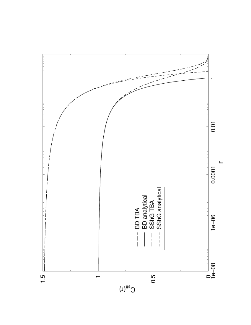
Figure 1: Plot of $c_{\rm eff}$ for the BD and the SShG models. $B=0.5$ for the BD model and $B=0.3$ for the SShG model.

We can do the similar analysis for the (NS) sector of the SShG model. We define the momentum $P$ in TBA framework as

$$P=\sqrt{\frac{1}{12}\left(\frac{3}{2}-c_{\rm eff}(r)\right)}\,,$$

and $\delta^{\rm(TBA)}$ as

$$\delta^{\rm(TBA)}(P)=\pi+2QP\ln{r\over{2\pi}}.$$

B	$\delta^{\rm(TBA)}_{1}$	$\delta^{\rm(SLFT)}_{1}$	$\delta^{\rm(TBA)}_{3}$	$\delta^{\rm(SLFT)}_{3}$	$\delta^{\rm(TBA)}_{5}$	$\delta^{\rm(SLFT)}_{5}$
0.1		–3.2785336087		21.66670467		–100.7910846
0.18	1.0670	1.06690190762	7.8	7.874361330		–18.38159324
0.2	1.63253	1.63252399743	6.50	6.511141559		–13.28563686
0.22	2.095776	2.09577590830	5.469	5.469890529	–9.6	–9.834738657
0.24	2.4799767	2.47997667482	4.65801	4.658037011	–7.41	–7.424651930
0.26	2.801552016	2.80155201512	4.014772	4.014774388	–5.697	–5.698671053
0.28	3.0723945744	3.07239457437	3.498766	3.498766117	–4.437	–4.437010555
0.3	3.3013090796	3.30130907959	3.0811053	3.081105362	–3.4992	–3.499327881
0.32	3.4949316196	3.49493161957	2.7411016	2.741101692	–2.7932	–2.793281686
0.34	3.6583334039	3.65833340390	2.4636642	2.463664336	–2.2565	–2.256567975
0.36	3.7954280414	3.79542804138	2.2376252	2.237625215	–1.8462	–1.846269137
0.38	3.9092523897	3.90925238965	2.0546356	2.054635580	–1.5323	–1.532335806
0.4	4.0021635972	4.00216359715	1.9084242	1.908424295	–1.29347	–1.293489949
0.42	4.07597900793	4.07597900793	1.7942911	1.794291077	–1.11458	–1.114593485
0.44	4.13207600398	4.13207600398	1.70875696	1.708756972	–0.98492	–0.984931878
0.46	4.17146289710	4.17146289710	1.64932333	1.649323338	–0.89708	–0.897087371
0.48	4.19482815387	4.19482815387	1.61430848	1.614308492	–0.84620	–0.846206262
0.5	4.20257268596	4.20257268596	1.60274253	1.602742538	–0.82954	–0.829542204

Table 2: First three coefficients of $\delta^{\rm(TBA)}$ in the expansion in powers of $P$ obtained by numerical analysis of the SShG model in comparison with the corresponding $\delta^{\rm(SLFT)}$ given by Eq.(3.2).

Table 2 shows the first three coefficients of $\delta^{\rm(TBA)}$ in the power expansion in $P$ obtained by numerical analysis of the SShG model and the corresponding $\delta^{\rm(SLFT)}$ given by Eq. (3.2) supplemented with the $\mu-m$ relation (20). Here again we see excellent agreements between the numerical and the analytical results. This result shows that the method based on the reflection amplitudes works perfectly in the presence of fermions like the SShG model. Especially the quantization condition for $P$ holds perfectly even for $b$ not small for which fermions interact nontrivially with bosons and the validity of the quantization condition may not be entirely clear at the first look. Thus our numerical result fully supports the analysis of TBA equations in sect. 4 and also the identification of undetermined constant $\beta$ as that coming from SLFT reflection amplitude. Actually, from the plot of $c_{\rm eff}(r)$ in Fig. 1, the approximation $c_{\rm eff}=3/2-12P^{2}$ is seen to work for larger region of $r$ than that in the BD case. The supression of ${\cal O}(r)$ correction might be related with the supersymmetric nature of the model.

6 Conclusion

In this paper we have analyzed the scaling functions of the ShG, the BD and the SShG models considered as integrable perturbations of the LFT and super-LFT using the reflection amplitudes and conventional TBA analysis. Our main result is that the new method based on the reflection amplitudes is not only consistent with the TBA but also necessary to completely understand the UV behaviour of the TBA. As our perturbative computations of the TBA show, there are no higher order corrections in the scaling functions except the leading correction which includes an unknown constant. To fix this constant, one should compare the scaling function obtained by the reflection amplitude, in particular the quantization conditions with the condition that the $L$ function in the TBA analysis be symmetric. Indeed, we identified the hidden condition in the TBA which are equivalent to the quantization condition. Our analytic results are fully supported by numerical studies where we have correctly reconstructed the reflection amplitudes from the TBA.

In addition, we find that the UV behaviours of the (NS) and (R) sectors in the SShG model are quite different. The scaling function of the (R) sector has only the power law perturbative corrections which vanish as $b\to 0$.

There are some interesting open problems which can be answered in a similar method used in this paper. First, our analysis of the ShG model, the $A^{(1)}_{1}$ affine Toda field theory, can be extended to those with higher rank by generalizing the one-dimensional quantum mechanical quantization condition to the higher-dimensional one [21].

Second, the new method to compute the scaling functions in terms of the reflection amplitudes can be extended to give the scaling behviour of the central charge of non-integrable models which can be expressed as perturbations of the LFT and super LFT. Previously, the scaling functions of the central charges can be computed only when the models are integrable so that one can use the TBA methods.

Another problem is to generalize the quantization condition and corresponding quantum mechanical interpretation so that the scaling function obtained in this way makes sense for the whole range of the scale $R$. To do this, one may need non-perturbative expression for the power corrections.

So far we have considered only the bulk integrable models. There has been much progress recently in the integrable models with boundaries. The main physical quantity which can be computed using boundary TBA is the boundary entropy which can also flow as the boundary scale varies. Using a similar logic presented in this paper, one may compute the scaling function of the boundary entropy using the reflection amplitudes of the boundary correlation functions for the boundary LFT [22].

We hope our approach made in this paper can provide an alternative approach to compute the scaling functions in the two dimensional quantum field theories.

References

• [1] A. B. Zamolodchikov, Int. J. Mod. Phys. A4 (1989) 4235.
• [2] Al. B. Zamolodchikov, Nucl. Phys. B342 (1990) 695.
• [3] A. B. Zamolodchikov and Al. B. Zamolodchikov, Nucl. Phys. B477 (1996) 577.
• [4] Al. B. Zamolodchikov, β€œResonance factorized scattering and roaming trajectories”, prepreint ENS-LPS-335, 1991.
• [5] M. J. Martins, Nucl. Phys. B394 (1993) 339.
• [6] A. Fring, C. Korff and B.J. Schulz, β€œThe ultraviolet Behaviour of Integrable Quantum Field Theories, Affine Toda Field Theory”, hep-th/9902011.
• [7] Al. B. Zamolodchikov, Int. J. Mod. Phys. A10 (1995) 1125.
• [8] P. Baseilhac and V. A. Fateev, Nucl. Phys. B532 (1998) 567; Al. B. Zamolodchikov, in private communications.
• [9] M. Goulian and M. Li, Phys. Rev. Lett. 66 (1991), 2051.
• [10] H. Dorn and H.-J. Otto, Phys. Lett. B291 (1992) 39; Nucl. Phys. B429 (1994) 375.
• [11] J. L. Gervais, Nucl. Phys. B391 (1993) 287.
• [12] V. A. Fateev, S. Lukyanov, A. B. Zamolodchikov, and Al. B. Zamolodchikov, Nucl.Phys. B516 (1998) 65.
• [13] R. C. Rashkov and M. Stanishkov, Phys. Lett. B380 (1996) 49.
• [14] R. H. Poghossian, Nucl.Phys. B496 (1997) 451.
• [15] T. Curtright and G. Ghandour, Phys. Lett. B136 (1984) 50.
• [16] P. Fendley, Nucl. Phys. B374 (1992) 667.
• [17] R. Shankar and E. Witten, Phys. Rev. D17 (1978) 2134.
• [18] C. Ahn, Nucl. Phys. B354 (1991) 57.
• [19] C. Ahn, Nucl. Phys. B422 (1994) 449; C. Ahn and C. Rim, to appear in J. Phys. A.
• [20] E. Witten, Nucl. Phys. B185 (1981) 513.
• [21] C. Ahn, C. Kim, C. Rim, and B. Yang, in preparation.
• [22] V. Fateev, S. Lukyanov, A. Zamolodchikov, and Al. Zamolodchikov, β€œExpectation values of boundary fields in the boundary sine-Gordon model”, hep-th/9807236.