Thermodynamic Stability and Phases of General Spinning Branes

Abstract

We determine the thermodynamic stability conditions for near-extreme rotating D3, M5, and M2-branes with multiple angular momenta. Critical exponents near the boundary of stability are discussed and compared with a naive field theory model. From a partially numerical computation we conclude that outside the boundary of stability, the angular momentum density tends to become spatially inhomogeneous.

Periodic Euclidean spinning brane solutions have been studied as models of QCD. We explain how supersymmetry is restored in the world-volume field theory in a limit where spin becomes large compared to total energy. We discuss the hierarchy of energy scales that develops as this limit is approached.

I Introduction

Mathematically, thermodynamic stability is equated with the subadditivity of the entropy function. More precisely, suppose the entropy $S$ is known in the microcanonical ensemble as a function of the other extensive thermodynamic variables (like energy and charge), which we will collectively denote $x_{i}$. Subadditivity of the function $S(\{x_{i}\})$ is the condition

$$S(\{\lambda x_{i}+(1-\lambda)\tilde{x}_{i}\})\geq\lambda S(\{x_{i}\})+(1-\lambda)S(\{\tilde{x}_{i}\})\ .$$ (1)

If the inequality went the other way, then the system could gain entropy by dividing into two parts, one with a fraction $\lambda$ of the energy, charge, etc., and the other with a fraction $1-\lambda$. When the system satisfies (1), no such process is allowed by the Second Law of Thermodynamics, and it is in this sense that the system is thermodynamically stable.

For black holes, perhaps a better way to think of (1) (though a more heuristic one) is as follows: (1) is satisfied for all $x_{i}$ and $\tilde{x}_{i}$ in a sufficiently small neighborhood of a given point in phase space if and only if it is possible for a black hole at that point to exist in thermal equilibrium with a heat bath much larger than itself. A simple example would be the Reissner-Nordström black hole in four-dimensional Einstein-Maxwell theory with no electrically charged particles. Near extremality, the specific heat is positive, but far from extremality the specific heat is negative. If one starts with the black hole in a state with positive specific heat and a temperature close to the temperature of some thermal gas of gravitons and photons, then the black hole will equilibrate with the thermal gas. On the other hand, if the black hole was in a state of negative specific heat, then even if its temperature is arbitrarily close to that of the thermal gas, the black hole will either emit faster than it absorbs or absorb faster than it emits, and correspondingly get smaller and hotter or bigger and colder. There is no bound on the runaway phenomenon except for the black hole to make the transition to positive specific heat or else to absorb most of the matter in the universe (assuming the universe is finite). That is what one means by instability of the initial configuration.

For spinning D- or M-branes, the heat bath line of reasoning is questionable because it is not clear whether one can construct an appropriate heat bath. One could perform the following gedanken experiment. Start with an array of nearly identical parallel spinning branes distributed through space, and ask whether, as they trade Hawking radiation among themselves, there is a process of equilibration or disequilibration among them. This is the standard trick of constructing an ensemble out of replicas of a given system. The branes should equilibrate precisely when (1) is satisfied. However, there is a difficulty: one has to estimate whether the time scale of equilibration or disequilibration is faster or slower than the time scale on which the gravitational forces between the replicas appreciably distort the array. Near the phase transition of [1], one expects the equilibration time scale to diverge, so the gedanken experiment will become impractical (even by the standards of gedanken experiments) close enough to the transition.

As a first step we can think of a single cluster of near-extreme coincident branes in a decoupling limit of the theory, where Hawking radiation to the asymptotically flat region of spacetime is very slow. Once we have analyzed the criterion (1) and established the existence of unstable solutions (even in this near-extreme decoupling limit), we can ask what form the instability takes. Because the branes have spatial extent, perhaps the most natural assumption is that the solutions which spin too fast are unstable against distributing their angular momentum unevenly across their worldvolume, somewhat analogous to the Gregory-Laflamme transition [2]. We will have more to say on this possibility in section III.

The work of [1] illustrates that the thermodynamics of the D3-brane world-volume theory, as read off from the Bekenstein-Hawking formula from the supergravity geometry, is stable only on a restricted region of phase space. That is, (1) is guaranteed to be satisfied only if the $x_{i}$ and the $\tilde{x}_{i}$ lie within the specified region. Our first goal, which we pursue in section II A, is to extend the stability analysis of [1] from one independent angular momentum to three, and to the case of near-extreme M5-branes and M2-branes with two and four angular momenta, respectively. (The maximum number of independent angular momenta is the rank of the rotation group perpendicular to the brane).

We will restrict ourselves to the near-extreme limit of spinning branes. For D3-branes, the string theory account of the microstates of the brane in terms of strongly coupled ${\cal N}=4$ super-Yang-Mills theory is thought to apply in this limit. The near-extremal spinning geometries have a near-horizon limit which is asymptotic to $AdS_{5}\times S^{5}$, so if we employ the philosophy of the AdS/CFT correspondence [3, 4, 5], we would say that the supergravity thermodynamics translates directly into a characterization of thermal states of the gauge theory. Instability is more of a surprise in this context, since statistical mechanical derivations of thermodynamics as a rule imply subadditivity of the entropy. The difficulty of treating the strongly coupled ${\cal N}=4$ gauge theory at finite temperature prevents us from deriving or disproving the instability from first principles. In section II C we do however extend the simplified field theory treatment introduced in [1] to the case of several angular momenta, and we show that the results are qualitatively similar to the supergravity predictions.

In section II B we discuss the supergravity predictions for critical exponents at the boundary of stability. The maximal number of fractional critical exponents at a given point on the boundary is the number of non-zero angular momenta. We show in section II C that similar critical exponents arise from the naive regulated field theory treatment for the D3-brane. Our analysis is not detailed on this point.

In section IV we analyze the supergravity solutions Wick-rotated to Euclidean time. We observe that the angular momentum amounts in field theory to a twist imposed on the $R$-charged fields in the field theory: the field theory partition function is altered from $\mathop{\rm tr}\nolimits e^{-\beta H}$ to $\mathop{\rm tr}\nolimits Re^{-\beta H}$ where $R$ is an element of the $R$-symmetry group. It describes the angle through which the brane spins during one period of the Euclidean time. In the limit discussed in [6] where angular momentum becomes large with energy held fixed, $R\to(-1)^{F}$, so we wind up with almost supersymmetric boundary conditions. For M5-branes compactified down to four dimensions, this leads to ${\cal N}=4$ super-Yang-Mills theory with supersymmetry slightly broken by boundary conditions in the Kaluza-Klein reduction. We review how the near-supersymmetry affects the proposals to use spinning branes as holographic approaches to QCD, and we note a puzzle regarding the energy scale of supersymmetry breaking and confinement.

II Thermodynamics of spinning branes

A Supergravity analysis

The supergravity solutions for spinning branes were constructed in [7]. The metric for the general spinning D3-brane and M5-brane can also be found in [9, 10] and [11], respectively. We are interested primarily in the thermodynamics, and this follows directly from the general formulas of [8].

Some parameters that enter into the thermodynamics of D3-, M2-, and M5-branes are shown in the following table:

brane $${p} {D} {T_{p}} {\alpha_{p}} {c_{p}} {3} {7} {{\sqrt{\pi}\over\kappa}} {2} {{1\over 8\pi^{2}}} {5} {6} {\left({\pi\over 2\kappa^{4}}\right)^{1/3}} {3} {{1\over 96\pi^{3}}} {2} {9} {\left({2\pi^{2}\over\kappa^{2}}\right)^{1/3}} {{\textstyle{3\over 2}}} {{1\over 3\sqrt{2}\pi}}$$ D3: M5: M2: (2)

In (2), $\kappa$ is the ten-dimensional gravitational coupling for the D3-brane, and the eleven-dimensional gravitational coupling for the M2-brane and the M5-brane. Using formulas (14) and (15) of [8], one finds the following expressions for the mass, charge, and spins of the branes:

$${M}$$

(3)

Our variables are defined in terms of those of [8] by

$$r_{0}^{D-3}=2m\qquad y_{i}={\ell_{i}\over r_{0}}\qquad y_{H}={r_{H}\over r_{0}}\ .$$ (4)

The location of the horizon, $y_{H}$, is the largest positive root of a cubic or quartic equation (obtained from (16) of [8]):

D3: $${{}(y^{2}+y_{1}^{2})(y^{2}+y_{2}^{2})(y^{2}+y_{3}^{2})-y^{2}=0} {{}(y^{2}+y_{1}^{2})(y^{2}+y_{2}^{2})-y=0} {{}(y^{2}+y_{1}^{2})(y^{2}+y_{2}^{2})(y^{2}+y_{3}^{2})(y^{2}+y_{4}^{2})-y^{2}=0}$$ M5: M2: (5)

It is useful to introduce one more combination of the parameters:

$$R^{D-3}\equiv r_{0}^{D-3}\cosh\alpha\sinh\alpha\ .$$ (6)

The constants $\alpha_{p}$ and $c_{p}$ were defined so that

$${\Omega_{D-2}\over N^{\alpha_{p}}2\kappa^{2}}=\left\{\vbox{\openup 3.0pt\halign{\strut\hfil$\displaystyle{#}$& $\displaystyle{{}#}$\hfil\cr&{c_{3}\over R^{8}}\qquad\hbox{for D3}\cr&{c_{p}\over R^{9}}\qquad\hbox{for M2 and M5.}\cr}}\right.$$ (7)

We can now define $E=M-Q$ and rewrite

$${e={E\over N^{\alpha_{p}}V}}$$

(8)

The approximate expressions are for the near-extreme limit, $\alpha\to\infty$ with $R$ held fixed. Scaling out the power $N^{\alpha_{p}}V$ from $E$, $J_{i}$, and $S$ allows us to write all subsequent expression in terms of $e$, $j_{i}$, and $s$ alone. That all powers of $V$ can be absorbed in this way is dictated by the absence of any scale in the theory; that all powers of $N$ can also be absorbed seems to be telling us that the effective number of degrees of freedom is on the order $N^{\alpha_{p}}$, as first conjectured in [12]. We can form dimensionless ratios

$${{s^{p+1}\over e^{p}}}$$

(9)

1 Grand-canonical ensemble

Now we wish to ask in what region of phase space $s$ is a sub-additive function of the energy density $e$ and the angular momentum densities $j_{i}$. We regard the $j_{i}$ as thermodynamic variables rather than fixed parameters, and the requirement of sub-additivity means that Legendre transforms with respect to the $j_{i}$ as well as with respect to $e$ are invertible. Thus, in the sense described in section III A of [13], we are investigating stability in the grand canonical ensemble. Stability in the canonical ensemble, where only the Legendre transform with respect to $e$ is required to be invertible, amounts to positivity of the specific heat, with the $j_{i}$ regarded as fixed parameters. We will treat stability in the canonical ensemble in section II A 2. We will exhibit evidence in section III that the grand-canonical ensemble is the relevant one when the world-volume is large. All of our actual calculations will be done in the microcanonical ensemble, that is writing $s=s(e,j_{i})$.

The function $y_{H}=y_{H}(y_{i})$ is complicated to express in closed form, since it is the solution of a cubic or a quartic equation, cf. (5). Using (9), we can write

$$s=2\pi\gamma e^{p/(p+1)}y_{H}\left({j_{i}\over\gamma e^{p/(p+1)}}\right)\ ,$$ (10)

where $\gamma^{p+1}=c_{p}2^{2p+1}/(D-1)^{p}$, and the arguments $y_{i}$ of $y_{H}$ have been written out explicitly in terms of the $j_{i}$. Fortunately, there is a more convenient way to judge the subadditivity of (10) than brute force. For instance, one can require that $e$ is concave up as a function of $s$ and the $j_{i}$. Or, most usefully, one can show that the domain of stability is the maximal region including the points where all $j_{i}=0$ where the temperature $T=\partial e/\partial s$ and the angular velocities $\Omega_{i}=\partial e/\partial j_{i}$ are one-to-one functions of $s$ and the $j_{i}$. This is the criterion we will actually use.

By differentiating the explicit expression (10) with respect to $j_{i}$, one can show that

$${\Omega_{i}\over T}=-2\pi{\partial y_{H}\over\partial y_{i}}\ .$$ (11)

It is useful to define the dimensionless ratios

$$x_{i}={y_{i}\over y_{H}}=2\pi{j_{i}\over s}\ .$$ (12)

Because of the scaling which follows from conformal invariance, any dimensionless thermodynamic quantity (like $e^{p}/s^{p+1}$) can be expressed in terms of the $x_{i}$. This is true in particular of $\Omega_{i}/T$: we have

$${\partial y_{H}\over\partial y_{i}}={x_{i}\over 1+x_{i}^{2}}W\qquad\hbox{where}\quad W={2\over 3-D+2\sum_{j=1}^{\left\lfloor{D-1\over 2}\right\rfloor}{x_{j}^{2}\over 1+x_{j}^{2}}}\ .$$ (13)

The sum over $j$ in $W$ is over all the independent angular momenta, of which there are $\lfloor(D-1)/2\rfloor$. The most straightforward way to prove (13) is to use the relations

$${y_{H}^{3-D}}$$

(14)

The first of these is a rephrasing of (5); the second follows from the first by logarithmic differentiation; and the third follows from (12) also by logarithmic differentiation. Again because of the various scaling laws, the relations $T=\partial e/\partial s$ and $\Omega_{i}=\partial e/\partial j_{i}$ are one-to-one if and only if (13) can be inverted to express the $x_{i}$ in terms of the $\partial y_{H}/\partial y_{i}$. At the boundary of a region of $x_{i}$-space on which (13) can be inverted, at least one of the eigenvalues of the matrix $\left[{\partial\over\partial x_{i}}{\partial y_{H}\over\partial y_{j}}\right]$ goes to zero or infinity. Provided we can show that $W$ is finite on the entire region of stability, its boundary will be given by the solution of $\det\left[{\partial\over\partial x_{i}}{\partial y_{H}\over\partial y_{j}}\right]=0$ closest to the origin, $x_{i}=0$. Extracting an overall factor of $W^{\lfloor(D-1)/2\rfloor}\prod_{k}{1\over 1+x_{k}^{2}}$, the determinant equation becomes

$$D(x_{i})\equiv\det\left[x_{i}{\partial\log W\over\partial x_{j}}+\delta_{ij}{1-x_{i}^{2}\over 1+x_{i}^{2}}\right]=0\ .$$ (15)

This determinant has a simple closed form:

$$D(x_{i})={(D-3)P(-1)+2P^{\prime}(-1)\over(D-3)P(1)-2P^{\prime}(1)}$$ (16)

where $P(\lambda)$ is defined by

$$P(\lambda)=\prod_{k}(1+\lambda x_{k}^{2})=1+\sum_{\ell=1}^{\left\lfloor{D-1\over 2}\right\rfloor}\lambda^{\ell}\sum_{i_{1}>i_{2}>\ldots>i_{\ell}}\prod_{j=1}^{\ell}x_{i_{j}}^{2}\ .$$ (17)

Note that $D(x_{i})=1$ when all the $x_{i}$ vanish. Thus the region of stability is the domain including $x_{i}=0$ where $D(x_{i})\geq 0$. If all but one angular momentum is zero, then

$$D(x)={(D-3)-(D-5)x^{2}\over(D-3)+(D-5)x^{2}}$$ (18)

Which indicates that the region of stability for a single angular momentum is $x^{2}\leq{D-3\over D-5}$. Apparently by coincidence, $\alpha_{p}={D-3\over D-5}$ as well. The bound $x^{2}\leq\alpha_{p}$ is in agreement with equation (17) of [1] in the case $p=3$, and with the bounds derived in [14] for $p=2$ and $p=5$.

It is straightforward to verify that the denominators of $W$ in (13) and $D(x_{i})$ in (15) differ only by a factor $-P(1)$, and that both these denominators are nonzero and finite throughout the domain including $x_{i}=0$ where the numerator of $D(x_{i})$ is positive. Thus an equivalent condition of stability to $D(x_{i})\geq 0$ is

$$(D-3)P(-1)+2P^{\prime}(-1)=(D-3)+\sum_{\ell=1}^{\left\lfloor{D-1\over 2}\right\rfloor}(-1)^{\ell}(D-3-2\ell)\sum_{i_{1}>i_{2}\cdots>i_{\ell}}\prod_{j=1}^{\ell}x_{i_{j}}^{2}\geq 0\ .$$ (19)

For the three types of branes we are considering, (19) specializes to

D3: $${{}2-x_{1}^{2}-x_{2}^{2}-x_{3}^{2}+x_{1}^{2}x_{2}^{2}x_{3}^{2}\geq 0} {{}3-x_{1}^{2}-x_{2}^{2}-x_{1}^{2}x_{2}^{2}\geq 0} {{}3-2(x_{1}^{2}+x_{2}^{2}+x_{3}^{2}+x_{4}^{2})} {{}\quad{}+(x_{1}^{2}x_{2}^{2}+x_{1}^{2}x_{3}^{2}+x_{1}^{2}x_{4}^{2}+x_{2}^{2}x_{3}^{2}+x_{2}^{2}x_{4}^{2}+x_{3}^{2}x_{4}^{2})} {{}\quad{}-x_{1}^{2}x_{2}^{2}x_{3}^{2}x_{4}^{2}\geq 0\ .}$$ M5: M2: (20)

Our methods can also be used to judge the stability of rotating black strings in five and six dimensions arising from intersections of spinning M-branes: $M5\perp M5\perp M5$ for five dimensions, and $M5\perp M2$ for six dimensions. Because the world-volume is effectively two-dimensional, one does not expect any phase transition at finite temperature, on account of the Mermin-Wagner theorem [15]. Indeed, it is straightforward to verify by direct computation that the entropy function is subadditive. It is also possible to trace through an analysis like the one in section II A, introducing a combination of parameters $R_{i}^{D-3}=r_{0}^{D-3}\cosh\alpha_{i}\sinh\alpha_{i}$ for each constituent family of branes, and verifying that (16) is always satisfied. (We note however that (19) is not always satisfied for the six-dimensional case: a zero in the denominator of (16) cancels a zero in the numerator.)

2 Canonical Ensemble

For the sake of completeness we also derive the subadditivity constraints for the canonical ensemble. This is the case where the angular momenta (“charges”) of rotating branes are kept fixed, so that subadditivity of the entropy is exactly equivalent to positivity of the specific heat at constant $j_{i}$. As we will demonstrate, it may be difficult to keep the $j_{i}$ uniform over the entire world-volume outside of the grand-canonical region of stability. However, uniform $j_{i}$ will be our working assumption in this section. It is a general result, demonstrated in section III A of [13] and verifiable directly from comparing (LABEL:canonical) to (20), that the region of stability in the canonical ensemble is larger than in the grand canonical ensemble. The canonical stability constraints for spinning branes with one angular momentum were first studied by Cai and Soh in [14].

Using (8), (9), (10), (13), and (14), it is fairly straightforward to reduce the inequality $\partial^{2}s/\partial e^{2}\leq 0$ to

$${\rm D3:}\ 2+5\sum_{i=1}^{3}x_{i}^{2}-\sum_{i=1}^{3}x_{i}^{4}+10\sum_{i<j}^{3}x_{i}^{2}x_{j}^{2}+16x_{1}^{2}x_{2}^{2}x_{3}^{2}+2\sum_{\{i<j\}\neq k}^{3}x_{i}^{2}x_{j}^{2}x_{k}^{4}$$ (22)

$$+3\sum_{\{i<j\}\neq k}^{3}x_{i}^{4}x_{j}^{4}x_{k}^{2}+5x_{1}^{4}x_{2}^{4}x_{3}^{4}\geq 0\ ,$$

$${\rm M5:}\ 9+36(x_{1}^{2}+x_{2}^{2})-9(x_{1}^{4}+x_{2}^{4})+76x_{1}^{2}x_{2}^{2}+8(x_{1}^{4}x_{2}^{2}+x_{2}^{4}x_{1}^{2})+21x_{1}^{4}x_{2}^{4}\geq 0\ ,$$ (23)

$${\rm M2:}\ 9+18\sum_{i=1}^{4}x_{i}^{2}+34\sum_{i<j}^{4}x_{i}^{2}x_{j}^{2}+60\sum_{i<j<k}^{4}x_{i}^{2}x_{j}^{2}x_{k}^{2}+2\sum_{i\neq j}^{4}x_{i}^{2}x_{j}^{4}-3\sum_{i<j}^{4}x_{i}^{4}x_{j}^{4}+6\sum_{\{i<j\}\neq k}^{4}x_{i}^{2}x_{j}^{2}x_{k}^{4}$$ (26)

$$+96x_{1}^{2}x_{2}^{2}x_{3}^{2}x_{4}^{2}\ -2\sum_{\{i<j\}\neq k}^{4}x_{i}^{4}x_{j}^{4}x_{k}^{2}+12\sum_{\{i<j<k\}\neq\ell}^{4}x_{i}^{2}x_{j}^{2}x_{k}^{2}x_{\ell}^{4}$$

$$+2\sum_{\{i<j\}\neq\{k<\ell\}}^{4}x_{i}^{4}x_{j}^{4}x_{k}^{2}x_{\ell}^{2}+6\sum_{\{i<j<k\}\neq\ell}^{4}x_{i}^{4}x_{j}^{4}x_{k}^{4}x_{\ell}^{2}+9x_{1}^{4}x_{2}^{4}x_{3}^{4}x_{4}^{4}\geq 0\ ,$$

where the $x_{i}$ are defined in (12).

A special case a single angular momentum turned on, say, $x_{1}=x\neq 0$, these stability constraints reduce to:

$${\rm D3}: \ 2+5x^{2}-x^{4}\geq 0\ ,$$ (28)

$${\rm M5}: \ 1+4x^{2}-x^{4}\geq 0\ ,$$ (29)

$${\rm M2}: \ 1+2x^{2}\geq 0\ .\,$$ (30)

which are identical to the constraints derived in [14]. Note that the M2-brane with a single angular momentum is always stable, but that with two angular momenta or more an instability is possible. (For example, when one approaches criticality along a special directions of $n$ equal non-zero angular momenta the critical values become $x_{c}\approx 2.118431$ and $x_{c}\approx 2.193567$ for $n=2$ and $n=3$, respectively.)

B Critical Exponents

We will focus on the grand canonical ensemble. Critical exponents characterize the behavior near a critical point of the grand potential, also called the Gibbs potential, and defined as $\Xi=E-ST-\sum_{i}\Omega_{i}J_{i}$. Conformal invariance implies $\Xi=-\textstyle{1\over p}E$. Using (8) and (9), one derives

$${\xi\equiv{\Xi\over{VN^{\alpha_{p}}}}=}$$

(31)

where $C={p^{p}\over{(p+1)^{p+1}}}(2\pi\gamma)^{p+1}$. One can also show that the inverse temperature of the solution is

$$\beta\equiv{1\over T}={{8\pi p}\over{(D-1)(p+1)}}R\left({R\over r_{0}}\right)^{{D-3}\over{p+1}}\prod_{i}(1+x_{i}^{2})^{1\over{3-D}}\left({{3-D}\over{3-D+2\sum_{j}{{x_{j}^{2}}\over{1+x_{j}^{2}}}}}\right)\ .$$ (32)

The expression (31) for $\xi$ is in terms of the $x_{i}$, and it is straightforward to make a Taylor expansion around a point $x_{ic}$ on the boundary of stability. There is no singular behavior in this expansion. However, if $\xi$ is expanded around the chosen point $x_{ic}$ in powers of $\Omega_{i}-\Omega_{ci}$, there are in general fractional critical exponents, $\gamma_{ci}$. This is possible when in the expansion

$${\omega_{i}-\omega_{ic}}$$

(33)

the first term on the right hand side vanishes. There will always be directions of approach in $x_{i}$-space where this term does vanish: $A_{ij}$ has vanishing determinant at the boundary of stability, and if we set $x_{i}=x_{ic}-\eta v_{i}$ where $A_{ij}v_{j}=0$, then

$$\omega_{i}-\omega_{ic} \sim c_{2}\eta^{2}+c_{3}\eta^{3}+\ldots$$ (34)

$$\xi-\xi_{c} \sim \tilde{c}_{2}\eta^{2}+\tilde{c}_{3}\eta^{3}+\ldots\ ,$$ (35)

for some coefficients $c_{i}$ and $\tilde{c}_{i}$. There is no linear term in $\eta$ in (34) by construction of $v_{i}$. There is also no linear term in (35) because such a term would cause some component of the angular momentum to become infinite as $\eta\to 0$, and this we can rule out with calculations in the microcanonical ensemble. Eliminating $\eta$ one can obtain an expansion for $\xi$ of the form

$$\xi\sim\hbox{(analytic)}+|\omega_{i}-\omega_{ic}|^{2-\gamma}+\ldots\ ,$$ (36)

where the term shown explicitly is the leading non-analytic term. In the absence of numerical coincidences such as the $\eta^{2}$ term vanishing in (34), or the relative coefficients between $\eta^{2}$ and $\eta^{3}$ being identical in (34) and (35), we will have $\gamma=1/2$. It is important to keep in mind that the exponent $\gamma$ is a function both of the particular point on the boundary of stability one is approaching and of the direction of approach. In the cases we have examined, generically $\gamma=1/2$ with some isolated exceptions which we will now describe.

Let us take set $n$ angular momenta equal, so that $x_{1}=\ldots=x_{n}=x$, and send $x$ to its critical value $x_{c}$ with the other $x_{i}$ vanishing. In this case the expression for the common value $\omega$ of $\omega_{i}\equiv{\Omega_{i}\over T}$ in terms of $x$ can be inverted explicitly, and it takes the form:

$$x=\textstyle{1\over{2n+3-D}}\left(-\textstyle{{2\pi}\over{\omega}}\pm[\left(\textstyle{{2\pi}\over{\omega}}\right)^{2}+(2n+3-D)(D-3)]^{1/2}\right),\ \$$ (37)

Half integer powers appear in the expansion of $x$ around $\Omega-\Omega_{c}$ when $(2n+3-D)(D-3)<0$, and this leads to $\gamma=1/2$. This situation obtains when $n=1$ for all $D$, and also for $n=2$ in the case of the M2-brane. In fact $n=1$ is essentially the generic case: approach to the boundary along a normal direction away from any special point. When $n>1$ for the D3-brane or the M5-brane, and when $n>2$ for the M2-brane, (37) leads to an expansion of $\xi$ which involves only integer powers of $\omega-\omega_{c}$.

On account of (33), there can be as many independent directions where $\gamma$ is fractional as there are independent vectors annihilated by $A_{ij}$. In order to determine when $A_{ij}$ in (33) has multiple zero eigenvalues, an efficient method is to determine the entire locus of points where the polynomials in (20) vanish. Let us call one of these polynomials $p(x_{i})$, and note that $p=\lambda_{1}\ldots\lambda_{n}$ up to a factor which is never $0$, where $\lambda_{i}$ are the eigenvalues of $A_{ij}|_{x_{k}=x_{kc}}$. The locus $p=0$ is the union of the vanishing sets of the $\lambda_{i}$. At a generic point on $p=0$, only one $\lambda_{i}=0$. Near a point of $p=0$ where the vanishing set of one eigenvalue crosses the vanishing set of another, the equation $p=0$ does not define a manifold; rather, it defines two or more manifolds crossing. We can find these points by solving $p=0$ and $dp\equiv\sum_{i=1}^{\left\lfloor{D-1\over 2}\right\rfloor}{{\partial p}\over{\partial x_{i}}}dx_{i}=0$ simultaneously. For the M5-brane, there is no solution: $f=0$ truly defines a manifold, and the two eigenvalues of $A_{ij}$ never simultaneously vanish. For the D3-brane and the M2-brane, the only solutions are where all $x_{i}^{2}=1$. For the D3-brane, this is a branch point where two sheets of $p=0$ cross, and correspondingly two eigenvalues of $A_{ij}$ vanish. For the M2-brane, three sheets of $f=0$ cross, so three eigenvalues of $A_{ij}$ vanish. In general, the number of eigenvalues vanishing at a branch point is indicated by the lowest degree term in the Taylor expansion of $p$ around the branch point: that is, the order of the branch point.

C Field theory analysis

In [1] a field theory analysis of spinning D3-branes was attempted, using the fact that transverse angular momentum on the brane amounted to R-charge. In this section we will extend the analysis from one angular momentum to three. We will also briefly consider the M2-brane and the M5-brane.

The on-shell degrees of freedom in a single D3-brane’s world-volume theory are two vector boson states (counting positive and negative helicity separately), six scalar states, and eight fermion states. The R-charges of these states are specified by vectors in the weight lattice of $SO(6)$. The on-shell degrees of freedom for a single M2-brane are eight scalar states and eight fermion states, with R-charges specified by weight vectors of $SO(8)$. The on-shell degrees of freedom for a single M5-brane are three self-dual two-form states, five scalar states, and eight fermion states, with R-charges specified by weight vectors of $SO(5)$. All these states are tabulated in equation (38):

on-shell D3-brane states,

$$SO(6)$$ quantum numbers

on-shell M2-brane states,

$$SO(8)$$ quantum numbers

For $p=2$, $3$, or $5$, let $\vec{\alpha}$ be a vector which runs over the sixteen $p$-brane weights given above, and set $s_{\vec{\alpha}}=1$ when the corresponding particle is a boson and $s_{\vec{\alpha}}=-1$ when it is a fermion. We will calculate in the grand canonical ensemble with “voltages” $\Omega_{1}$, $\Omega_{2}$, …, $\Omega_{\lfloor(D-1)/2\rfloor}$ corresponding to the elements of the Cartan subalgebra of the R-symmetry group (for instance, in the case of D3-branes, we have $\Omega_{1}$, $\Omega_{2}$, and $\Omega_{3}$ for the three elements of the Cartan subalgebra of $SO(6)$). Denoting $\vec{\omega}=(\omega_{1},\omega_{2},\ldots,\omega_{\lfloor(D-1)/2\rfloor})$ where $\omega_{i}=\Omega_{i}/T$, we have in analogy to (26) of [1] an expression

$$\xi=T\int{d^{p}k\over(2\pi)^{p}}\sum_{\vec{\alpha}}s_{\vec{\alpha}}\log(1-s_{\vec{\alpha}}e^{-\beta|\vec{k}|+\vec{\alpha}\cdot\vec{\omega}})=-{T^{p+1}\Gamma(p)\over 2^{p-1}\pi^{p/2}\Gamma(p/2)}\sum_{\vec{\alpha}}s_{\vec{\alpha}}\mathop{\rm Li}\nolimits_{p+1}(s_{\vec{\alpha}}e^{\vec{\alpha}\cdot\vec{\omega}})$$ (39)

for the grand potential per unit volume, $\xi$, which is also the pressure. As in the case of only one angular momentum, the integrals diverge for any real nonzero $\vec{\omega}$ because there are charged massless bosons. The integrals in (39) are all special cases of

$$\int_{0}^{\infty}dk\,k^{n-1}\log(1-e^{\mu-k})=-\Gamma(n)\mathop{\rm Li}\nolimits_{n+1}(e^{\mu})\ ,$$ (40)

which is carried out assuming complex $\mu$ and using analytic continuation. The difficulty in defining the integrals for real $\vec{\omega}$ is apparent from the branch cuts across the positive real $\mu$ axis of $\mathop{\rm Li}\nolimits_{p+1}(e^{\mu})$. In [1] it was proposed to define the integrals using the principle value prescription, which in this case amounted to replacing the polylogarithms by their real parts. This prescription together with the identity

$$\mathop{\rm Li}\nolimits_{n}(e^{\mu})+(-1)^{n}\mathop{\rm Li}\nolimits_{n}(e^{-\mu})=\sum_{j=0}^{\lfloor n/2\rfloor}{2\zeta(2j)\over(n-2j)!}\mu^{n-2j}\pm{i\pi\over(n-1)!}\mu^{n-1}\ .$$ (41)

leads to

$$-{\xi\over T^{4}}\equiv g(\vec{\omega})={\pi^{2}\over 6}+{1\over 4}\sum_{i}\omega_{i}^{2}+{1\over 32\pi^{2}}\left(\sum_{i}\omega_{i}^{2}\right)^{2}-{1\over 16\pi^{2}}\sum_{i}\omega_{i}^{4}$$ (42)

for the D3-brane, and to

$${-{\xi\over T^{6}}}$$

(43)

for the M5-brane. For the M2-brane, the grand potential is transcendental, and cannot be simplified substantially beyond (39). At small $\omega_{i}$ one has the expansion

$$-{\xi\over T^{3}}={7\zeta(3)\over\pi}-\sum_{i}{\omega_{i}^{2}\over 4\pi}\left(\log{\omega_{i}^{2}\over 4}-3\right)+\ldots\ .$$ (44)

For $N$ coincident D3-branes branes in the supergravity limit, the world-volume theory is strongly interacting. We nevertheless suggest (42) as a first approximation to the grand potential of $3+1$-dimensional ${\cal N}=4$ $SU(N)$ gauge theory at high temperature, where now we have scaled a factor of $N^{2}$ out of $\xi$ as in section II A. The speculation is that even though the fundamental excitations are strongly interacting, for the purposes of thermodynamics we can think of $O(N^{2})$ quasi-particle excitations which have the same multiplet structure as the fundamental degrees of freedom. For the M2-brane, agreement with supergravity requires $O(N^{3/2})$ quasi-particles, whereas for the M5-brane, $O(N^{3})$ are required. These peculiar scalings are borne out by absorption calculations [16], but are otherwise poorly understood.

For the rest of this section we will focus on the D3-brane.

Thermodynamic stability requires that $\xi$ be a subadditive function of $T$ and the $\Omega_{i}$. Because of the scaling laws due to conformal invariance, this amounts to being able to express the $\omega_{i}$ as single-valued functions of the ratios $j_{i}/s$. It is straightforward to check that this is possible on the region of $\omega$ space containing the origin where

$$\det\left(4g{\partial^{2}g\over\partial\omega_{k}\partial\omega_{\ell}}-3{\partial g\over\partial\omega_{k}}{\partial g\over\partial\omega_{\ell}}+\omega_{i}{\partial g\over\partial\omega_{k}}{\partial^{2}g\over\partial\omega_{i}\partial\omega_{\ell}}-\omega_{i}{\partial g\over\partial\omega_{i}}{\partial^{2}g\over\partial\omega_{k}\partial\omega_{\ell}}\right)\geq 0\ .$$ (45)

In (45), which generalizes (42) of [1], the index $i$ is summed over in the last two terms, and $k$ and $\ell$ are the indices of the $3\times 3$ matrix whose determinant is taken.

The mean field theory analysis of [1] also generalizes in a simple way. We will omit some details which do not depend on the number of angular momenta. The basic idea is that there is some “self-field” contribution to the voltage, which we express as

$$\varphi=\omega+f(j/T^{3})\ .$$ (46)

Here $\varphi$ is the total voltage, $\omega$ is the applied voltage, and $f(j/T^{3})$ is the self-field contribution, given in terms of an unknown function $f$, and in terms of an R-charge density $j$ obtained by integrating over the thermal occupation factors (using the principle value prescription) in the presence of the total voltage $\varphi$. For notational simplicity we have dropped the arrows from $\varphi$, $\omega$, and $j$, but they are indeed three-dimensional vectors, and derivatives with respect to them are also three-dimensional vectors. Thus the permeability $\mu=\partial\varphi/\partial\omega$ is a $3\times 3$ matrix which can depend on $\omega$. The simplest extension of [1] is to assume $f(x)=-x$, which implies that the permeability at zero voltage is $\mu={\textstyle{2\over 3}}{\bf 1}$. That is, the D3-brane responds diamagnetically to an applied voltage. We will show how this ansatz reproduces the critical behavior found in supergravity.

Mean field theory leads to a parametric expression for the free energy:

$${-{\xi\over T^{4}}}$$

(47)

The first line in (47) uses (39) with $\omega$ replaced by $\varphi$. The second line is a rephrasing of (46) using the ansatz $f(x)=-x$. The function $g(\varphi)$ is the same as appeared in (42). Since $g(\varphi)$ is analytic, the only way nonanalyticity can arise is through inverting the relation between $\omega$ and $\varphi$. Nonanalyticity can arise in this context only if the inverse permeability,

$$\mu^{-1}={\partial\omega\over\partial\varphi}={\bf 1}+{\partial^{2}g\over\partial\varphi^{2}}\ ,$$ (48)

acquires a zero eigenvalue. Thus the boundary of stability is determined by $\det\mu^{-1}=0$, which is equivalent to

$${{}576\pi^{6}-48\pi^{4}(\varphi_{1}^{2}+\varphi_{2}^{2}+\varphi_{3}^{2})-20\pi^{2}(\varphi_{1}^{4}+\varphi_{2}^{4}+\varphi_{3}^{4})}$$

(49)

This complicated expression reduces to $|\varphi_{1}|\leq 2\pi$ when $\varphi_{2}=\varphi_{3}=0$. It exhibits the same qualitative behavior as (20), in that the boundary of stability is a generically a single zero of the left hand side, with the sole exception of all $\varphi_{i}^{2}$ equal, when the boundary of stability becomes a double zero. As before, this indicates that generically only one eigenvalue crosses through $0$ at the boundary, but for all angular momenta equal two eigenvalues vanish at the same time. We obtain the same critical behavior from the mean field theory analysis as from the supergravity, and for basically the same reasons: making the expansions

$${\omega-\omega_{c}}$$

(50)

we see that $\gamma=1/2$ for variations of $\omega$ in the directions in which $\mu^{-1}$ has a zero eigenvalue, while $\gamma=0$ in the other directions. The algebra is the same as in (34) and (35), except that there $\eta$ represented a deviation parametrized in terms of $x-x_{c}$, whereas in (50) it would be a deviation parametrized in terms of $\varphi-\varphi_{c}$.

III Phase mixing

So far our goal has been to demonstrate that spinning branes with a sufficiently high angular momentum become thermodynamically unstable. We have not answered the obvious question: what form does the instability take? In this section we will entertain two possibilities: 1) the branes fragment and fly apart in the transverse dimensions; and 2) the angular momentum density localizes on the branes. For the sake of specificity, we will focus exclusively on $N$ coincident D3-branes with only one angular momentum. In the notation of [1],

$$\chi={27\pi^{2}\over 8N^{2}}{(J/V)^{4}\over(E/V)^{3}}>{1\over 3}$$ (51)

puts us outside the region of stability as calculated in the grand canonical ensemble.

The naive expectation is that D3-branes with $\chi>1/3$ vigorously shed their angular momentum by radiating either closed strings or individual D3-branes. In an examination of the radial potentials for closed string emission and for equatorial motion of a test D3-brane in the background of $N$ spinning D3-branes, we found no evidence for a special unstable mode developing at $\chi=1/3$. This is not necessarily a problem: as commented upon in the introduction, the nature of the instability is not so much that there is some runaway mode of the system by itself, but rather that it is impossible to establish equilibrium between it and a heat bath.

The following simple estimate suggests that for $\chi>1/8$ D-brane fragmentation is thermodynamically allowed. Suppose the the $N$ D3-branes split into $k$ equal fragments. As the fragments fly apart, they can acquire orbital angular momentum. As an idealization of this complicated dynamical fission process, let us suppose that most of the angular momentum winds up in the orbital motion of the fragments, and that most of the energy winds up in their non-extremality. As a further idealization, we will assume that the process occurs uniformly across the D3-brane world-volume. By compactifying the world-volume on a small $T^{3}$ one could ensure such uniformity. From [1] we take the formula

$$s(e,j;N)={2^{5/4}3^{-3/4}\sqrt{\pi N}e^{3/4}\over\sqrt{\sqrt{1+\chi}+\sqrt{\chi}}}$$ (52)

for the entropy per unit world-volume in terms of the energy and angular momentum per unit world-volume. Since we will be considering different values of $N$, we have reverted to the conventions of [1]: $e=E/V$, $j=J/V$, and $s=S/V$, without the factors of $N^{2}$ in the denominator which we used in section II A. The ratio of the entropy of the final state ($k$ identical non-spinning fragments) to the initial state (a single cluster with spin) is

$${s_{f}\over s_{i}}={ks\left({e\over k},0;{N\over k}\right)\over s(e,j;N)}=\sqrt{{\sqrt{1+\chi}+\sqrt{\chi}\over\sqrt{k}}}\ .$$ (53)

The process is entropically favored if $s_{f}>s_{i}$, which is equivalent to $\sqrt{k}\leq\sqrt{1+\chi}+\sqrt{\chi}$. Kinematics forbids the $k=1$ process, so we get the lowest critical $\chi$ from $k=2$ (two fragments): $\chi>1/8$, as advertised. With $k=3$ (three fragments) we get $\chi>1/3$, which coincidentally corresponds exactly to the boundary of the domain where $s(e,j)$ is subadditive. Making the fragments unequal only increases the bound. For very large $\chi$, large values of $k$ will be accessible, and we interpret the fragmentation as a Jeans instability of the disk of D3-branes described in [9].

The above estimate does not convince us that brane fragmentation is the dominant instability for $\chi$ slightly larger than $1/3$. We would be more optimistic if an instability of the horizon could be identified. In any case, brane fragmentation would violate singularity theorems, so we may expect it to have a very long time-scale in the classical limit of many coincident branes.

We now turn to the second possibility: that for $\chi>1/3$ the angular momentum density $j$ tends to localize on the world-volume. If they are thermodynamically permitted, inhomogeneities in $j$ might nucleate locally on a shorter time-scale than brane fragmentation. In fact, the time scale should be on the order of the inverse temperature since there is no other scale in the problem.

Let us regard (52) as an approximate expression for the entropy density in terms of energy density $e$ and angular momentum density $j$ which are allowed to vary over the world-volume. Diffusion and interactions will tend to keep the temperature $T$ and the “voltage” $\Omega$ (properly the angular velocity at the black hole horizon) spatially constant. However, for a given $(T,\Omega)$, there are two possible values for energy density and angular momentum density. (That there are two and only two possible values can be seen from the fact that the equation of state, (20) of [1], is double-valued). One of them, call it $(e,j)$, will lie in the stable region where $s$ is subadditive; the other, call it $(\tilde{e},\tilde{j})$, will lie in the unstable region. Thus we are led to consider mixed states of the two phases $(e,j)$ and $(\tilde{e},\tilde{j})$. We will argue that such states are entropically favored over states with uniform $(e,j)$ for $\chi\mathrel{\mathstrut\smash{\ooalign{\raise 2.5pt\hbox{$>$}\cr\lower 2.5pt\hbox{$\sim$}}}}0.325$, although only for $\chi>1/3$ can a uniform state evolve smoothly into such a mixed state. The mixed states are only saddle points of the entropy functions, not maxima, because they involve an unstable component.

We emphasize that the following calculation is not on the same footing as the usual analysis of phase coexistence, because one “phase” in the current context is unstable. Rather, it is intended as a preliminary probe of how inhomogeneous $e$ and $j$ may arise near $\chi=1/3$, based on the idea that $T$ and $\Omega$ should remain at least approximately uniform while these inhomogeneities are first forming. Because we are relying on the known supergravity solutions as our guide to the thermodynamics, we are not equipped to address the questions of coherence length, surface tension, and stability of phase boundaries. Ideally, one would like to establish the existence of a second stable phase, perhaps one where the branes are separated in the transverse dimensions. Then a more standard equilibrium analysis would become possible.

Assume that a fraction $\lambda$ of the spatial volume is filled by the unstable phase $(\tilde{e},\tilde{j})$, and the remaining fraction $1-\lambda$ is filled by the stable phase, $(e,j)$. Then the average energy density, angular momentum density, and entropy density are

$${e_{av}}$$

(54)

where $s(e,j;N)$ is the function (52). With $e_{av}$ and $j_{av}$ fixed we want to extremize $s_{av}$ by varying $\lambda$. That is, in an isolated system where the total energy and angular momentum are fixed, we extremize the total entropy by distributing energy and angular momentum optimally between the two phases. This problem is mathematically well-posed because $\tilde{e}$ and $\tilde{j}$ can be determined as functions of $e$ and $j$, and then the first two lines of (54) amount to two (non-linear) constraints on three variables, leaving $\lambda$ as the only free variable.

More explicitly, for given $(T,\Omega)$, there are two solutions to the equations

$${\left(\partial s\over\partial j\right)_{e}}$$

(55)

and if one of them is $(e,j)$, then the other, $(\tilde{e},\tilde{j})$, can be expressed as

$${{}\tilde{e}=e\left({1+\chi\over 1+\tilde{\chi}}\right)^{4}{\tilde{\chi}\over\chi}\ ,\quad\tilde{j}=j\left({1+\chi\over 1+\tilde{\chi}}\right)^{3}{\tilde{\chi}\over\chi}}$$

(56)

With the help of (56) one can show that

$$s(\tilde{e},\tilde{j};N)=s(e,j;N)\left({1+\chi\over 1+\tilde{\chi}}\right)^{5/2}\left({\tilde{\chi}\over\chi}\right)^{1/2}\ .$$ (57)

Because of the overall scale invariance of the theory, it is equivalent to extremize

$$\sigma_{av}={s_{av}^{4}\over e_{av}^{3}}$$ (58)

with fixed

$$\chi_{av}={27\pi^{2}\over 8N^{2}}{j_{av}^{4}\over e_{av}^{3}}\ .$$ (59)

Using (54), (56), and (57), one can obtain $\sigma_{av}$ and $\chi_{av}$ explicitly as functions of $\chi$ and $\lambda$. The domain of $\chi$ is $[0,1/3]$ because it is by assumption the ratio pertaining to the stable component, and the domain of $\lambda$ is $[0,1]$. We have verified numerically that the contours of constant $\chi_{av}$ can be written as single-valued functions, $\lambda=\lambda_{\chi_{av}}(\chi)$. Thus the entropy along a given contour is extremized when

$$\left({\partial\sigma_{av}\over\partial\chi}\right)_{\chi_{av}}=\left({\partial\sigma_{av}\over\partial\chi}\right)_{\lambda}-\left({\partial\sigma_{av}\over\partial\lambda}\right)_{\chi}{\left({\partial\chi_{av}/\partial\chi}\right)_{\lambda}\over\left({\partial\chi_{av}/\partial\lambda}\right)_{\chi}}=0\ .$$ (60)

In figure 1 we show contours of constant $\chi_{av}$ cut by a dashed line indicating the solution set of (60).

From figure 1 one can conclude that for $\chi_{av}>1/3$ the entropically preferred state, among states with uniform temperature and voltage, is a mix of the stable and unstable phases, with $\lambda\mathrel{\mathstrut\smash{\ooalign{\raise 2.5pt\hbox{$>$}\cr\lower 2.5pt\hbox{$\sim$}}}}0.46$ and $\lambda\to 1$ as $\chi_{av}\to\infty$. The $\chi_{av}\mathrel{\mathstrut\smash{\ooalign{\raise 2.5pt\hbox{$<$}\cr\lower 2.5pt\hbox{$\sim$}}}}0.322$ mixtures are always entropically disfavored: for such $\chi_{av}$ the preferred state has $\lambda=0$. There is a narrow band of values, $0.322\mathrel{\mathstrut\smash{\ooalign{\raise 2.5pt\hbox{$<$}\cr\lower 2.5pt\hbox{$\sim$}}}}\chi_{av}<1/3$, where there are two far-separated competing states (see figure 2): one has $\lambda=0$ and one has $\lambda\approx 0.46$. At $\chi_{av}\approx 0.325$ there is a “transition” where $\lambda$ jumps from $0$ to $0.46$. The temperature and voltage also jump at this transition.

We regard this as preliminary evidence that there is a first order phase transition at a value of $\chi_{av}$ strictly less than $1/3$. The critical behavior associated with the boundary of stability would be cut off finitely below the critical angular momentum by phase separation. A more definitive treatment would be possible if one could identify a thermodynamically stable phase into which the system falls when the angular momentum density is sufficiently high. Our treatment has assumed that this new stable phase is very slow to form compared to the time-scale on which small inhomogeneities in $j$ can nucleate. This is reasonable if the new stable phase is some version of a multi-center solution, because passing to such a phase would violate classical singularity theorems.

In [14] it was proposed that in the canonical ensemble, stability persisted up to $\chi\approx 1.26$. As a general rule we agree that thermodynamic stability of a system depends on its environment. However the results of this section indicate that the instability of spinning D3-branes at $\chi=1/3$ is not easily avoided by changing ensembles. Consider a state with total $e$ and $j$ arranged so that $\chi_{av}$ is just slightly larger than $1/3$. The pure phase state would correspond to where one of the grey lines in figure 1 intersects the top of the frame. At this point, $\tilde{\chi}=\chi_{av}$. This is the sort of state that the authors of [14] regard as stable in the canonical ensemble (though not in the grand canonical ensemble). However, the system may increase its entropy continuously by flowing down along one of the grey lines, until it reaches the dashed black line, where entropy is a maximum at least among two-component mixed phase states of the prescribed $\chi_{av}$. In other words, the putatively stable state represents only a saddle point of the entropy, not even a local maximum. This is in contrast with states with $0.325\mathrel{\mathstrut\smash{\ooalign{\raise 2.5pt\hbox{$<$}\cr\lower 2.5pt\hbox{$\sim$}}}}\chi_{av}<1/3$, where a system in a pure phase state can increase its entropy only by making a big leap, all the way along one of the fine black lines from the bottom of the frame to the

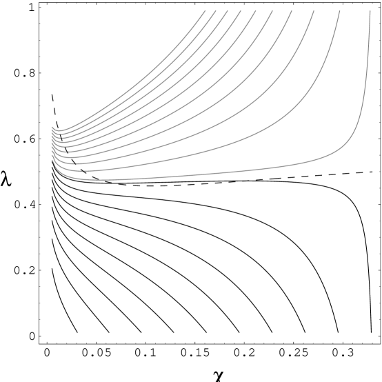
FIG. 1.: The solid black lines are contours of constant $\chi_{av}$ with $\chi_{av}<1/3$. The grey lines are contours of constant $\chi_{av}$ with $\chi_{av}>1/3$. The dashed line is the solution set of (60). The region below the dashed line is where entropy along a contour increases as one moves to larger $\chi$. If a contour intersects the dashed line, then the maximum of the entropy function along that contour is at the first intersection with the dashed line; otherwise the maximum is at the lower border $\lambda=0$.

FIG. 2.: The dimensionless ratio $\sigma_{av}=s_{av}^{4}/e_{av}^{3}$ is plotted against $\chi$ for two values of $\chi_{av}$ on either side of the phase transition: in a) $\chi_{av}=0.324$ while in b) $\chi_{av}=0.326$. In a) we see that the $\chi=0.324$, $\lambda=1$ solid phase wins out entropically; in b) the mixed phase with $\chi\approx 0.075$ and $\lambda\approx 0.46$ is entropically favored.

leftmost intersection of the fine black line with the dashed black line. In a nutshell, the pure phase states represented by the bottom of the frame in figure 1 are metastable against separation into a two-component mixture, but the pure phase states represented by the top of the frame are not even metastable. These statements are independent of the environment because we are talking only about shifting energy around within the world-volume of the D3-branes. The key point is that D3-branes have spatial extent, so any little bit of it can be regarded as a “system” in thermal contact with a “heat bath” consisting of the rest of the brane. That is what makes the grand canonical ensemble relevant. With black holes the story is different: because there is no spatial extent, it is doubtful that one can regard one part of the black hole as a heat bath for another part. If the D3-brane world-volume were compactified on a scale smaller than the thickness of a domain wall between phases, then the situation would be physically indistinguishable from a black hole, and calculations in the canonical ensemble might become relevant.

IV Euclidean Spinning Branes

A Spin and thermal boundary conditions

Euclidean black brane solutions can be obtained from the Minkowskian ones by sending $t\to-it$ and $\ell_{j}\to i\ell_{j}$, where the $\ell_{j}$ are the angular momentum parameters that enter into the solutions of [8]. Complexifying them is necessary in order to keep the $dtd\phi$ parts of the metric real. The consequences for the thermodynamics can all be reasoned out from the fact that the angular momentum becomes complex. In brief, one can retain equations (3) through (14) with the replacements $y_{j}\to iy_{j}$ and $x_{j}\to ix_{j}$, but $y_{H}\to y_{H}$ with no factor of $i$. These replacements have a profound effect on the physics: as we shall now argue, the phase space is $|x_{j}|<1$, and points on the boundary correspond to supersymmetric periodicity conditions in the Euclidean path integral.

The new version of the first equation in (14) is

$$y_{H,E}^{3-D}=\prod_{j}(1-x_{j}^{2})\ .$$ (61)

This relation becomes singular when any of the $x_{i}$ reaches $1$ in absolute value, so the phase space is indeed the cube $|x_{i}|<1$. The new version of (11) and (13) is

$${\Omega_{j}\over T}=2\pi i{\partial y_{H}\over\partial y_{j}}=-2\pi i{x_{j}\over 1-x_{j}^{2}}{2\over 3-D-\sum_{k}{2x_{k}^{2}\over 1-x_{k}^{2}}}\ .$$ (62)

We now want to study the limits of (62) as we approach the boundary of the cube. Consider fixing some number of the $x_{j}$ at values finitely far from the horizon and then letting all the others approach the horizon at the same rate: for these others, say $x_{j}=s_{j}(1-\epsilon)$ where $s_{j}=\pm 1$ and $\epsilon\to 0$. For convenience define $s_{j}=0$ for all the $x_{j}$ whose values are fixed in the interior. Let the number of $x_{j}$’s which are approaching the boundary be $n$. Approaching a generic point on the boundary corresponds to $n=1$; $n>1$ means one is approaching a point on an edge or a corner of the cube rather than a face. It is simple to see from (62) that

$${\Omega_{j}\over T}\to{2\pi i\over n}s_{j}\ .$$ (63)

For example, if we send $x_{1}\to 1$ and hold all the other $x_{i}$ fixed, then $\Omega_{1}/T\to 2\pi i$ and all other $\Omega_{j}/T\to 0$.

To understand what is happening in the world-volume theory, let us first recall that in the absence of rotation, the usual thermal partition function, $Z=\mathop{\rm tr}\nolimits e^{-\beta H}$, can be computed by a Euclidean path integral with period $1/T$ for Euclidean time. Boundary conditions on fermions are anti-periodic. To add real angular momentum—the kind that we have studied in all the previous sections—one would introduce a chemical potential $\vec{\Omega}$ for particles with R-charge: acting on a state $|\vec{\alpha}\rangle$ whose R-charge is specified by the vector $\vec{\alpha}$ in the weight space of the R-symmetry group, the hamiltonian $H$ would be replaced by $H-\vec{\alpha}\cdot\vec{\Omega}$ (cf. (39)). But in this section we are studying Euclidean angular momentum, which corresponds to pure imaginary $\vec{\Omega}$. Thus

$$e^{\vec{\alpha}\cdot\vec{\Omega}/T}|\vec{\alpha}\rangle=e^{\vec{H}\cdot\vec{\Omega}/T}|\vec{\alpha}\rangle=R|\vec{\alpha}\rangle\ ,$$ (64)

where $\vec{H}=(H_{1},H_{2},\ldots,H_{\lfloor(D-1)/2\rfloor})$ is a basis of generators for the Cartan subalgebra. $R=e^{\vec{H}\cdot\vec{\Omega}/T}$ is an element of the compact R-symmetry group $SO(D-1)$ (or more precisely its covering group) when $\vec{\Omega}$ is pure imaginary. The net effect of turning on $\vec{\Omega}$, as we see from (64), is to insert $R$ into the partition function: instead of $Z=\mathop{\rm tr}\nolimits e^{-\beta H}$, now we have $Z=\mathop{\rm tr}\nolimits Re^{-\beta H}$. In the Euclidean path integral, $R$ just specifies a twist in $SO(D-1)$ which one performs on all the fields before identifying from $t_{E}=1/T$ to $t_{E}=0$. This twist modifies the usual (thermal) boundary conditions according to the R-charge of each field.

If we set $\Omega_{1}/T=2\pi i$ and all other $\Omega_{j}/T=0$, then $R=(-1)^{F}$, where $F=0$ for bosons and $1$ for fermions. That is, we recover supersymmetric boundary conditions. Maximal Poincaré supersymmetry is recovered in this case because $R\eta=-\eta$ for any spinor $\eta$ of $SO(D-1)$. This does not mean that conformal invariance is recovered. In fact it is not: the near-horizon geometry is not anti-de Sitter for Euclidean spinning branes, even in the large spin limit we are considering. We are led to conclude that the geometry must be describing a physical state analogous to those considered in [9], where Higgs VEV’s break conformal invariance.

For $n>1$, we can judge whether any part of supersymmetry is restored by determining whether there are any spinors $\eta$ of $SO(D-1)$ which satisfy $R\eta=-\eta$, where $R$ is the element of the covering group of $SO(D-1)$ specified by $\Omega_{j}/T=2\pi i/n$ for $1\leq j\leq n$. It is straightforward to verify in this way that a fraction $(1/2)^{n-1}$ of supersymmetry is preserved in all cases except $n=4$ for the M2-brane, where $1/4$ of supersymmetry is preserved.

By studying Killing spinor equations in the spinning brane supergravity geometries one can confirm the presence of unbroken supersymmetry. This was essentially done in [18] for the M2-brane. To be more precise, [18] includes an investigation of the Killing spinor equations for BPS-saturated R-charged black holes of $N=8$ $D=4$ gauged supergravity. The results of [19, 13] indicate that Kaluza-Klein reduction of spinning M2-branes leads precisely to large R-charged black holes of the type studied by the authors of [18]. They found that $2^{5-n}$ supersymmetries are preserved by black holes with $n=1$, $2$, or $3$ charges, while adding a fourth charge does not break any additional supersymmetry. This counting is in agreement with the previous paragraph: for example $n=1$ corresponds to $16$ supersymmetries, which is the maximum when conformal symmetry is broken by the physical state.

The weight vectors listed in (38) can be used to determine the allowed momenta $k_{E}$ around the Euclidean $S^{1}$. These momenta determine tree-level masses in the dimensionally reduced theory. For $n<4$ there is Bose-Fermi degeneracy in all cases (M2, D3, and M5). (See also figure 3.) The M2-brane with $n=4$ exhibits no Bose-Fermi degeneracy. This may be an indication that our description of the world-volume theory of many M2-branes in terms of excitations with the same $SO(8)$ quantum numbers as for a single M2-brane is too simplistic to capture even the rough outlines of the field theory.

In order to further shed light on the nature of supersymmetry restoration in field theory and to make comparison with the supergravity results, let us turn to the study of the thermodynamic quantities.

We obtain $\Omega_{j}/T=(2\pi i)/n$ exactly when $x_{i}=\pm 1$ ($i=1,\cdots,n$), but other thermodynamic relations become singular in this limit. So we choose $\omega_{i}=(\pm){2\pi i}/[n(1-\epsilon)]$ ($x_{i}=\pm(1-\epsilon)$) ($i=1,...,n$, $\epsilon\ll 1$), and for the sake of simplicity we set other $\omega_{j}$’s to zero. This is still not the most general way one could imagine approaching the boundary of phase space: for instance, one could set $x_{i}=\pm(1-r_{i}\epsilon)$ with arbitrary but fixed $r_{i}$. This does not lead to any more general scaling behavior than what we will observe, but the coefficients in equations (65) through (74) and (80) would change.

First we compute the grand potential for the field theory obtained from (39) with the supersymmetric particle content given in (38). The field theory results in the $\epsilon\to 0$ limit are as follows:

$${\rm D3:} \ \ \ {\xi\over T^{4}}=-\pi^{2}\left(\textstyle{2\over 3}\epsilon^{3}\ ,\textstyle{1\over 2}\epsilon^{2}\ ,\textstyle{4\over{27}}\epsilon\ \right),\ \ n=(1,2,3)\ ,$$ (65)

$${\rm M5:} \ \ \ {\xi\over T^{6}}=-\pi^{3}\left(\textstyle{1\over 3}\epsilon^{4}\ ,\textstyle{1\over{12}}\epsilon^{2}\,\right)\ ,\ \ \ n=(1,2)\ ,$$ (66)

$${\rm M2:} \ \ \ {\xi\over T^{3}}=-\left(\pi\ln{2}\ \epsilon^{2}\ ,\pi(\textstyle{3\over 2}+\ln{2\over{\pi\epsilon}})\epsilon^{2}\ ,2.0988\epsilon\ ,0.33480\,\right)\ ,\ \ \ n=(1,2,3,4)\ .$$ (67)

For a single M5-brane, or D3-brane this field theory analysis is sound: it amounts simply to counting states in a free field theory. (It is not even plagued by the divergences that we used the principle value prescription to solve in section II C: those divergences were for $\omega_{i}$ real, and are completely avoided by pure imaginary $\omega_{i}$.) For $N>1$ our understanding of the field theory at finite temperature is limited. The naive approach is to hope that it has some properties in common with $O(N^{3})$ copies [$O(N^{2})$ copies] of the $N=1$ theory in the M5- [D3-] brane. This approach is not well motivated physically, but it does give the correct scalings with $N$ and $\epsilon$ as predicted by supergravity. The field theory on multiple M2-branes not very well understood. It is based on a particular infrared limit of the D2-brane gauge theory where $SO(8)$ symmetry is thought to be recovered (see for example [20, 21]). For a single brane, a simple Hodge dualization of a vector field into a scalar field suffices to show this, but for multiple branes there does not seem to be a simple argument directly from field theory.

The positive powers of $\epsilon$ in (65)-(66) appear because of the Bose-Fermi degeneracy in the spectrum of allowed $k_{E}$. This is substantially the only indicator of supersymmetry in this free field theory computation.

Let us now compare the field theory results to those obtained in supergravity. There the grand potential $\xi$ is given by (31). In the $\epsilon\to 0$ limit, $\xi$ has the following scaling behavior:

$$\xi\sim T^{p+1}\epsilon^{{{n(p+1)}\over{3-D}}+p+1}\ .$$ (68)

The specific results are:

$${\rm D3:} \ \ \ {\xi\over T^{4}}=-\pi^{2}\left(16\epsilon^{3}\ ,\textstyle{1\over 2}\epsilon^{2}\ ,\textstyle{4\over{81}}\epsilon\ \right)\ ,\ n=(1,2,3)\ ,$$ (69)

$${\rm M5:} \ \ \ {\xi\over T^{6}}=-\pi^{3}\left(\textstyle{16\over 3}\epsilon^{4}\ ,\textstyle{1\over{48}}\epsilon^{2}\ \right)\ ,\ \ \ n=(1,2)\ ,$$ (70)

$${\rm M2:} \ \ \ {\xi\over T^{3}}=-\pi^{2}\left(\textstyle{64\over{3}}\epsilon^{5/2}\ ,\textstyle{{4\sqrt{2}}\over{3}}\epsilon^{2}\ ,\textstyle{32\over 81}\epsilon^{3/2}\ ,\textstyle{1\over{6\sqrt{2}}}\epsilon\ \right)\ ,\ n=(1,2,3,4)\ .$$ (71)

It is instructive to trace the behavior the inverse temperature in this limit. Using the expression (32) one obtains:

$${\rm D3:} \ \ \ \beta\equiv{1\over T}={{2\pi}\over n}{R^{2}\over r_{0}}(2\epsilon)^{1-{n\over 4}}\ ,\ n=(1,2,3)\ ,$$ (72)

$${\rm M5:} \ \ \ \beta\equiv{1\over T}={{2\pi}\over n}\left({R^{3}\over r_{0}}\right)^{1\over 2}(2\epsilon)^{1-{n\over 3}}\ ,\ \ \ n=(1,2)\ ,$$ (73)

$${\rm M2:} \ \ \ \beta\equiv{1\over T}={{2\pi}\over n}{R^{3}\over r_{0}^{2}}(2\epsilon)^{1-{n\over 6}}\ ,\ n=(1,2,3,4)\ .$$ (74)

Note that for finite temperature to remain finite $r_{0}\sim(\epsilon^{1-{n\over 4}}\ ,\epsilon^{{6-2n}\over 3}\ ,\epsilon^{{6-n}\over{12}})$ for D3-, M5- and M2-brane, respectively.

Comparing the supergravity results (69) through (71) with those the field theory analysis ((65) through (67)) reveals that except for rational prefactors the supergravity and field theory results are in good qualitative agreement for both D3- and M5-brane, as expected since a single D3- and M5-brane field theory analysis is believed to be sound. On the other hand there is a qualitative discrepancy between the two approaches for the M2-brane case, again indicating that the field theory of M2-brane is poorly understood.

Most importantly, we see that the energy density $e=-p\xi$ scales in all cases with a positive power of $\epsilon$. Recall that $e$ is the energy density over and above the energy density of a BPS-saturated brane configuration. By the same argument that zero energy states in a supersymmetric theory are supersymmetric states, we conclude that a state with $e=0$ preserves at least some of the original supersymmetries of the brane.

We would like to conclude this subsection by commenting on the supergravity analysis of the spectrum of the theory. This will become relevant in our discussion in the next subsection of models of confinement based on spinning branes. Let us concentrate on a minimally coupled scalar $\phi$, that is a scalar whose linearized equation of motion is the Laplace equation in the background of the Euclidean spinning brane:

$${1\over{\sqrt{-g}}}\partial_{\mu}(\sqrt{-g}g^{\mu\nu})\partial_{\nu}\phi=0.$$ (75)

With the ansatz $\phi=e^{ikx}\chi(r)$, where $x$ is a world-volume direction, and (for the sake of simplicity) $\chi(r)$ depends only on the radial coordinate $r$, one obtains a radial equation of the following form:

$$D\ \ {\rm odd}: \ \ \ {1\over rR^{D-3}}\partial_{r}\left[r^{-1}\prod_{i=1}^{\left\lfloor{{D-1}\over 2}\right\rfloor}(r^{2}-\ell_{i}^{2})-2mr\right]\partial_{r}\chi(r)=k^{2}\chi(r)\ ,$$ (76)

$$D\ \ {\rm even}: \ \ \ {1\over rR^{D-3}}\partial_{r}\left[\prod_{i=1}^{\left\lfloor{{D-1}\over 2}\right\rfloor}(r^{2}-\ell_{i}^{2})-2mr\right]\partial_{r}\chi(r)=k^{2}\chi(r)\ .$$ (77)

These wave equations were derived in [10] and [11] for the D3-brane and the M5-brane, respectively. In the field theory, the values of $|k|$ will be masses of $O^{++}$ glueballs.

In terms of the notation introduced in this paper these wave equations assume the form:

$$D\ \ {\rm odd}: \ \ \ {x}^{-1}\partial_{x}\left[y_{H}^{D-3}x^{-1}\prod_{i=1}^{\left\lfloor{{D-1}\over 2}\right\rfloor}(x^{2}-x_{i}^{2})-x\right]\partial_{x}\chi=y_{H}^{2}(kr_{0})^{2}\left({R\over r_{0}}\right)^{D-3}\chi\ ,$$ (78)

$$D\ \ {\rm even}: \ \ \ x^{-1}\partial_{x}\left[y_{H}^{D-3}\prod_{i=1}^{\left\lfloor{{D-1}\over 2}\right\rfloor}(x^{2}-x_{i}^{2})-x\right]\partial_{x}\chi=y_{H}^{2}(kr_{0})^{2}\left({R\over r_{0}}\right)^{D-3}\chi\ .$$ (79)

Our radial variable is $x={r\over r_{0}y_{H}}$. The quantities $x_{i}$, $y_{i}$, $y_{H}$, $r_{0}$, and $R$ were introduced at the beginning of section II A, but because we are now operating in Euclidean space we must recall the replacements $x_{j}\to ix_{j}$ and $y_{j}\to iy_{j}$. When $n$ equal Euclidean angular momenta becoming large at fixed energy (that is, $x_{i}\to\pm(1-\epsilon)$ for $i=1\ldots,n$), the limiting behavior for $k$ is

$$k\equiv M_{\rm glueball}={\textstyle{{2\pi}\over n}}{\cal Q}(2\epsilon)^{1-{n\over 2}}T\ ,\ \ (n=1,\cdots,{\textstyle{{[D-1]}\over 2}})\ ,$$ (80)

where $T$ is the Hawking temperature (32)  (which at the boundary takes the values (72)-(74)), and ${\cal Q}$ is a pure number determined by the following eigenvalue equation:

$$D\ \ {\rm odd}: \ \ \ {x}^{-1}\partial_{x}\left[x^{-1}\prod_{i=1}^{\left\lfloor{{D-1}\over 2}\right\rfloor}(x^{2}-x_{i}^{2})\right]\partial_{x}\chi=-{\cal Q}^{2}\chi,$$ (81)

$$D\ \ {\rm even}: \ \ \ x^{-1}\partial_{x}\left[\prod_{i=1}^{\left\lfloor{{D-1}\over 2}\right\rfloor}(x^{2}-x_{i}^{2})\right]\partial_{x}\chi=-{\cal Q}^{2}\chi\ ,$$ (82)

where now $x_{i}^{2}=1$ $(i=1,\ldots,n)$ and other $x_{j}$’s are set to zero. (As before, with non-zero $x_{j}^{2}\neq 1$’s and $x_{i}=\pm(1-r_{i}\epsilon)$, the equations (82) are of the same form, and the mass gap (80) has the same scaling behavior with $\epsilon$, but the actual numerical prefactors in (80) change.) Discrete eigenvalues ${\cal Q}$ arise from demanding that $\chi$ is normalizable.

Thus $M_{gap}\sim\sqrt{\epsilon}T$ for $n=1$, $M_{gap}\sim T$ for $n=2$, and $M_{gap}$ diverges for $n>2$. For $n>2$ it is possible that there is actually no discrete spectrum in the $\epsilon\to 0$ limit. This point is under investigation.

The mass gap can also be quantified in terms of the ratios of the angular momentum densities at the boundary, $j_{i}$, ($i=1,\cdots,n$) and $e$. It is straightforward to obtain the following scaling behavior: $j_{i}\sim T^{p}\epsilon^{{{n(p+1)}\over{3-D}}+p}$. One can easily show that

$$M_{gap}\sim\left({j_{i}^{2}\over e}\right)^{1/(p-1)}\sim T\epsilon^{1-{n(p+1)\over(D-3)(p-1)}}=T\epsilon^{1-{n\over 2}}\ .$$ (83)

Some of the observations we have made about the scaling of the mass gap and about supersymmetry restoration also follow easily from the results of [22, 6, 10, 11]. The connection that does not seem to have been made there is that the field theory itself recovers supersymmetry in the limit of small $\epsilon$ because of the insertion of an element of the R-symmetry group into the partition function.

B Models of confinement

The usual route to $\hbox{QCD}_{4}$ [23] is to compactify the M5-brane worldvolume on a circle twice. The first time, one uses supersymmetric boundary conditions on a circle of circumference $2\pi R_{1}$, and by the M-IIA duality the result is a D4-brane which, like the M5-brane, is near-extreme. The second compactification is applied to the Euclidean time coordinate of the D4-brane: it has period $1/T$, and we impose thermal rather than supersymmetric boundary conditions. This second compactification is the important step. The five-dimensional theory one is starting with on the D4-brane is the Euclidean version of the $SU(N)$ gauge theory with maximal supersymmetry which descends from the ten-dimensional ${\cal N}=1$ supersymmetric Yang-Mills theory. The resulting theory in four dimensions will also have $SU(N)$ gauge fields, but no supersymmetry, and it is the candidate for $\hbox{QCD}_{4}$. Tracing through the M-IIA relationship determining the string coupling in terms of the compactification radius $R_{1}$, and then the relationships between the string coupling, the D4-brane gauge coupling, and the four-dimensional $\hbox{QCD}_{4}$ coupling $g_{YM}^{2}$, one finds $g_{YM}^{2}=2\pi R_{1}T$. The relevant points for our analysis are: 1) the compactification process is unchanged when there is angular momentum in the directions orthogonal to the M5-brane; 2) the ’t Hooft coupling $\lambda=g_{YM}^{2}N$ needs to be large for the supergravity to be valid.

When there is no angular momentum, the fermions are anti-periodic in the Euclidean time used in the $\hbox{D4}\to\hbox{QCD}_{4}$ compactification, so in the four-dimensional lagrangian they have masses $\pi T$. It is usually assumed that at large ’t Hooft coupling, the scalars pick up comparable masses. From supergravity one learns that the mass gap is also of order $T$. This is sensible from a field theory point of view: in the renormalization group flow of a gauge theory in which the ’t Hooft coupling is large at energies comparable to the masses of the matter fields, one expects confinement at only lower energies. This is to be contrasted with a gauge theory where the ’t Hooft coupling is weak at energies comparable to the masses of the lightest matter fields. There we have the standard one-loop relation $M_{\rm gap}\sim\exp\left({-{8\pi^{2}\over b_{0}g_{YM}^{2}}}\right)m_{\rm matter}$, and $b_{0}={11\over 3}N$.

When there is a large angular momentum, or, in the parlance of section IV A, small $\epsilon$, the story is rather different. The fermion masses are not all on the order of the temperature: as indicated in figure 3, some of them are on the order of $\epsilon T$.

FIG. 3.: The spectrum of momenta in the compactified $S^{1}$ direction of the D4-brane world volume. The larger ticks indicate bosons; the smaller ticks indicate fermions. The first line follows from standard thermal boundary conditions. The second and third lines show what happens when one approaches the boundary of the phase space (large angular momentum for fixed energy), either at an edge ($n=1$) or a corner ($n=2$). The splittings in these cases are on the order $\epsilon T$. In the close groupings of ticks in the second and third lines, the degeneracies follow the ratios $1:4:6:4:1$ and $1:2:1$, respectively.

Supersymmetry is restored in the limit $\epsilon\to 0$. In the $n=1$ case, for energies much smaller than $T$, only the center grouping of modes is available, and the theory is four-dimensional ${\cal N}=4$ super-Yang-Mills. In the $n=2$ case, the center group of states fills out the ${\cal N}=2$ super-Yang-Mills multiplet.

Supergravity calculations which we summarized in the previous subsection indicate that the scaling of the mass gap is $M_{\rm gap}\sim\sqrt{\epsilon}T$ for $n=1$ and $M_{\rm gap}\sim T$ for $n=2$. Near the end of this section we explain why this scaling is rather at odds with our field theory expectations. For now we will regard the scaling of $M_{\rm gap}$ as a non-trivial prediction of supergravity.

In view of the existence of matter fields comparable to or much lighter than the scale of confinement, it is no surprise that large angular momenta did not suffice to decouple the “glueballs” charged under the global symmetry group which rotates these quarks among themselves [6]. The existence of such “Kaluza-Klein cousins” has been a persistent feature of all supergravity models of $\hbox{QCD}_{4}$, but it need not be regarded as an artifact of the construction which must disappear in a full string theory treatment. In any confining gauge theory (including real-world QCD) in which there are fundamental matter fields with some flavor symmetry and with masses comparable to or lighter than the confinement scale, one expects to have flavored hadrons as well as flavor-neutral glueballs. It may not be reasonable to hope that a full string theory treatment of these backgrounds will decouple all matter fields and leave us with pure glue. It seems more likely that it will leave us with confining glue coupled to light matter.

It makes sense that glueball mass ratios should be roughly the same [11] when one makes one angular momentum large as when one makes two large in any ratio except unity. In terms of the $x_{i}$ variables discussed in the section IV A and defined in (12), an M5-brane with one angular momentum large with the other zero corresponds to $x_{1}\to 1$ while $x_{2}=0$, whereas two large angular momenta with fixed ratio corresponds to $x_{1}\to 1$ with $x_{2}/x_{1}=\eta$. As long as $\eta\neq 1$, one is approaching the edge rather than the corner of the square which represents the phase space of the spinning brane, and the pattern of tree-level masses shown in figure 3 obtains. Glueball mass ratios should be and are approximately independent of $\eta$ because the matter fields whose tree-level masses are small in comparison with the confinement scale. When $\eta=1$, the pattern of tree-level masses is as shown in the $n=2$ line of figure 3. We expect that glueball mass ratios will change at this point because the relevant matter fields have changed their tree-level masses.

One difficulty with the original proposal of [23] is that the scale of the fifth dimension is the same as the scale of confinement. Thus any process whose energy is high enough to probe the gauge dynamics non-trivially—in the sense that colored states, not just an effective theory like soft pions, would be needed to analyze the process—would also probe the fifth dimension. One might therefore ask in what sense one has defined a four-dimensional gauge theory at any scale. The spinning branes construction is better in this regard because for $n=1$ there is a large range of energies, $\sqrt{\epsilon}T\ll E\ll T$, where the theory is four-dimensional and unconfined. The decoupling [6] of “glueballs” with Kaluza-Klein momentum in the fifth dimension is the tangible evidence that the length of the fifth dimension is much smaller than the inverse QCD scale.

Other approaches to confinement avoid a fifth dimension altogether by using only D3-branes, either in type 0 theory [24] or with a varying dilaton in type IIB theory [25] (see also [26]. These models have their own difficulties: in the former the gravity description breaks down in the ultraviolet, and there is a tachyon whose mass is on the string scale; while in the latter one seems to need some excited string state to start the dilaton flowing, and asymptotic freedom cannot be achieved. Both approaches involve naked singularities in the bulk.

We summarize the taxonomy of holographic approaches to confining gauge theories in figure 4. The basic features of confinement are not expected to depend on the existence of matter fields or on their masses, provided that the beta function remains negative. All the gravity models have a string tension which is much larger than the square of the mass gap. This leads to some behaviors very unlike real QCD [27], in particular nearly flat Regge trajectories. In figure 4, we have indicated only the mass gap—that is, the mass scale seen by closed string probes. In all cases except 3), the QCD string tension would be located between this mass scale and the next highest scale; in 3) the relation of the QCD string tension and the temperature can only be determined given the relative sizes of $\epsilon$ and the ’t Hooft coupling $g_{YM}^{2}N$.

Since only one large angular momentum is needed to make the scalings we have discussed, it should be possible to construct variants of the spinning M5-brane approach by putting the branes at some spacetime singularity. Orbifold backgrounds would be expected to lead to bifundamental quarks rather than adjoints. There might even be chiral models analogous to those discussed in [28]. A model with bona-fide light fundamental quarks could be difficult to construct, since the fundamental representation is the charge carried by one end of a string ending on a D-brane, and not typically by an open string with both its ends on the brane.

There is one outstanding difficulty: why for $n=1$ is the confinement scale much higher than the tree-level masses of the light matter fields ($\sqrt{\epsilon}T\gg\epsilon T$)? The most obvious resolution would be for at least some of the light masses to receive radiative corrections on the order $\sqrt{\epsilon}T$ from diagrams where heavy fields run around loops.

FIG. 4.: Energies scales in various attempts to find a supergravity dual to confining gauge theories. Also included for purposes of comparison is a cartoon sketch of real-world QCD and a generic lattice model. The quark masses shown are the parameters that enter into the lagrangian: constituent masses.

If this were to happen, then superconformal invariance would be broken at a scale on the order of $\sqrt{\epsilon}T$, and confinement would follow at an energy scale only slightly lower. But the following simple estimate suggests that perturbative effects cannot generate a sufficiently large radiative correction. Scalar mass renormalizations at one loop typically arise from integrals of the form

$$F(M)=\int{d^{4}q\over(2\pi)^{4}}{1\over q^{2}+M^{2}}={M^{2}\over 8\pi^{2}}\log{M\over\mu}\ ,$$ (84)

where we have used dimensional regularization and the minimal subtraction scheme. $M$ is the mass of the heavy fields running around the loop. Typically, in a theory with supersymmetry broken by mass splittings for the heavy fields on the order $\Delta M$, we have $\delta m^{2}\sim(\Delta M)F^{\prime}(M)\sim(\Delta M)M\log{M\over\mu}$ on account of the near-cancellation of bosonic and fermionic contributions. With mass breakings such as the ones indicated in figure 3, the cancellation is even better: $\delta m^{2}\sim(\Delta M)^{\cal N}F^{({\cal N})}(M)$ where ${\cal N}$ is the degree of supersymmetry restored when $\Delta M=0$. In particular, $\delta m^{2}\sim\epsilon^{4}T$ for $n=1$, where ${\cal N}=4$ supersymmetry is restored in the $\epsilon\to 0$ limit.

Although perturbation theory seems to have failed, we find it plausible that the heavy fields should play a role in setting the scale of supersymmetry breaking at $\sqrt{\epsilon}T$. This scale is just the geometric mean of the tree-level masses of the light and heavy fields, but its relevance to the dynamics may emerge in field theory only through features peculiar to strong coupling gauge interactions.

To summarize our discussion: In no sense should spinning M5-brane solutions with a large angular momentum be regarded as the analog of improved lattice actions for pure $\hbox{QCD}_{4}$. The fermions’ tree level masses are not all far above the confinement scale. In fact, some of them are far smaller than this scale. We do not understand the field theory mechanism that sets the scale of supersymmetry breaking and confinement at $O(\sqrt{\epsilon}T)$ for the case of one large angular momentum. However, if we take this scaling as a given, we do understand why glueball mass ratios should be universal for two large unequal angular momenta and somewhat different when they are equal: it is because the pattern of supersymmetry breaking is universal in the first case, but different in the second. It would be delightful if the near-restoration of supersymmetry could be exploited to make more definite predictions about the confining dynamics than is possible for pure $\hbox{QCD}_{4}$.

The D3-brane with periodic Euclidean time has been proposed as a model for pure $\hbox{QCD}_{3}$ [23]. Without angular momentum, the bare three-dimensional fermion masses and also the mass gap are on the order of $T$. With $n$ equal large Euclidean angular momentum, the light fermion masses are $m_{\rm bare}\sim\epsilon T$, whereas the mass gap is $M_{\rm gap}\sim\epsilon^{1-{n\over 2}}T$ for $n=1$ or $2$. Again it is not easy to see what in field theory sets this confinement scale. Universality of glueball mass ratios can be understood in a similar way to the four-dimensional case, but we regard it as a more pressing problem to understand the overall scaling of the mass gap from a field theory perspective.

The supergravity analysis of the previous subsection applies to Euclidean spinning M2-branes as well. However, in view of the poor understanding of the large $N$ field theory we refrain from drawing any further comparisons.

V Conclusion

The purpose of this paper was to provide a comprehensive study of the thermodynamics of spinning D3-, M5-, and M2-branes. Our results address the following aspects:

• Thermodynamic Stability and Critical Behavior

  We derived general stability constraints for near-extreme D3-, M5- and M2-branes, all with the maximum number of independent spins. The region where the entropy is subadditive as a function of both the energy and the angular momenta is strictly smaller than the region where the specific heat is positive. To illustrate one of the possible instabilities that develops when the entropy is not subadditive, we studied states where the angular momentum is unevenly distributed over the world volume, and found them to be entropically preferred over the uniform distribution despite the fact that they are not themselves stable configurations.

• Field Theory

  We generalized the field theory model of [1] to the case of multiple R-charges; the dynamics is proposed to be described effectively by a collection of weakly interacting massless “quasi-particles” whose R-charges and spins are those of the abelian theory on a single brane. If one assumes in a addition that there is a nonzero “permeability” for applied “voltages” dual to the various R-charges, then this model reproduces the critical behavior of the supergravity analysis.

• Euclidean spinning branes

  Euclidean branes with at least one angular momentum density which is large compared to the energy density restore some fraction of supersymmetry. We showed how this supersymmetry restoration arises in the field theory: an element of the R-symmetry group is inserted in the partition function, which for one large spin approaches $(-1)^{F}$. The spectrum is nearly supersymmetric, with the Bose-Fermi degeneracy broken by $\Delta M\sim\epsilon T$, where $\epsilon$ is a dimensionless parameter that goes to zero in the limit of large angular momentum. The supergravity analysis reveals that if there is confinement, it occurs on a scale $M_{gap}\sim T\epsilon^{1-n/2}$ when $n$ equal Euclidean angular momenta are made large. We have explained how this picture elucidates some of the results of previous papers [6, 11]. We have left open the problem of identifying the field theory mechanism that sets the scale of supersymmetry breaking.

REFERENCES

- [1] S. S. Gubser, “Thermodynamics of spinning D3-branes,” hep-th/9810225.
- [2] R. Gregory and R. Laflamme, “Black strings and p-branes are unstable,” Phys. Rev. Lett. 70 (1993) 2837, hep-th/9301052.
- [3] J. Maldacena, “The Large N limit of superconformal field theories and supergravity,” Adv. Theor. Math. Phys. 2 (1998) 231, hep-th/9711200.
- [4] S. S. Gubser, I. R. Klebanov, and A. M. Polyakov, “Gauge theory correlators from noncritical string theory,” Phys. Lett. B428 (1998) 105, hep-th/9802109.
- [5] E. Witten, “Anti-de Sitter space and holography,” Adv. Theor. Math. Phys. 2 (1998) 253, hep-th/9802150.
- [6] C. Csaki, Y. Oz, J. Russo, and J. Terning, “Large N QCD from rotating branes,” hep-th/9810186.
- [7] M. Cvetič and D. Youm, “Rotating intersecting M-branes,” Nucl. Phys. B499 (1997) 253, hep-th/9612229.
- [8] M. Cvetič and D. Youm, “Near BPS saturated rotating electrically charged black holes as string states,” Nucl. Phys. B477 (1996) 449–464, hep-th/9605051.
- [9] P. Kraus, F. Larsen, and S. P. Trivedi, “The Coulomb branch of gauge theory from rotating branes,” hep-th/9811120.
- [10] J. Russo and K. Sfetsos, “Rotating D3 branes and QCD in three dimensions,” hep-th/9901056.
- [11] C. Csaki, J. Russo, K. Sfetsos, and J. Terning, “Supergravity models for (3+1)-dimensional QCD,” hep-th/9902067.
- [12] I. R. Klebanov and A. A. Tseytlin, “Entropy of near extremal black p-branes,” Nucl. Phys. B475 (1996) 164–178, hep-th/9604089.
- [13] M. Cvetič and S. S. Gubser, “Phases of R charged black holes, spinning branes and strongly coupled gauge theories,” hep-th/9902195.
- [14] R.-G. Cai and K.-S. Soh, “Critical behavior in the rotating D-branes,” hep-th/9812121.
- [15] N. D. Mermin and H. Wagner, “Absence of ferromagnetism or antiferromagnetism in one- dimensional or two-dimensional isotropic Heisenberg models,” Phys. Rev. Lett. 17 (1966) 1133–1136.
- [16] S. S. Gubser and I. R. Klebanov, “Absorption by branes and Schwinger terms in the world volume theory,” Phys. Lett. B413 (1997) 41–48, hep-th/9708005.
- [17] D. Z. Freedman, S. S. Gubser, K. Pilch, and N. P. Warner, “Continuous distributions of d3-branes and gauged supergravity,” hep-th/9906194.
- [18] M. J. Duff and J. T. Liu, “Anti-de Sitter black holes in gauged N = 8 supergravity,” hep-th/9901149.
- [19] A. Chamblin, R. Emparan, C. V. Johnson, and R. C. Myers, “Charged AdS black holes and catastrophic holography,” hep-th/9902170.
- [20] S. Sethi and L. Susskind, “Rotational invariance in the M(atrix) formulation of type IIB theory,” Phys. Lett. B400 (1997) 265–268, hep-th/9702101.
- [21] N. Seiberg, “Notes on theories with 16 supercharges,” Nucl. Phys. Proc. Suppl. 67 (1998) 158, hep-th/9705117.
- [22] J. G. Russo, “New compactifications of supergravities and large N QCD,” hep-th/9808117.
- [23] E. Witten, “Anti-de Sitter space, thermal phase transition, and confinement in gauge theories,” Adv. Theor. Math. Phys. 2 (1998) 505, hep-th/9803131.
- [24] J. A. Minahan, “Asymptotic freedom and confinement from type 0 string theory,” hep-th/9902074.
- [25] S. S. Gubser, “Dilaton driven confinement,” hep-th/9902155.
- [26] A. Kehagias and K. Sfetsos, “On running couplings in gauge theories from type IIB supergravity,” hep-th/9902125.
- [27] D. J. Gross and H. Ooguri, “Aspects of large N gauge theory dynamics as seen by string theory,” Phys. Rev. D58 (1998) 106002, hep-th/9805129.
- [28] A. M. Uranga, “Brane configurations for branes at conifolds,” hep-th/9811004.