hep-th/9903108

IPM/P-99/012

March 1999

Branes at Angles from DBI Action
R. Abbaspur

Institute for Studies in Theoretical Physics and Mathematics,
P.O. Box 19395-5531, Tehran, Iran.
Department of Physics, Sharif University of Technology,
P. O. Box 19365-9161, Tehran, Iran.

In this paper we investigate about several configurations of two intersecting branes at arbitrary angles. We choose the viewpoint of a brane source and a brane probe and use the low-energy dynamics of p-branes. For each p-brane this dynamics is governed by a generic DBI action including a WZ term, which couples to the SUGRA background of the other brane. The analysis naturally reveals two types of configurations: the “marginal” and the “non-marginal” ones. We specify possible configurations for a pair of similar or non-similar branes in either of these two categories. In particular, for two similar branes at angles, this analysis reveals that all the marginal configurations are specified by $SU(2)$ angles while the non-marginal configurations are specified by $Sp(2)$ angles. On the other hand, we find that no other configuration of two intersecting branes at non-trivial angles can be constructed out of flat p-branes. So in particular, two non-similar branes can only be found in an orthogonal configuration. In this case the intersection rules for either of the marginal or non-marginal configurations are derived, which thereby provide interpretations for the known results from supergravity.

1 Introduction

Intersecting branes at arbitrary angles have been studied both in view of their SUSY properties in supergravity [3, 2, 1, 4, 5] and their short-range interactions in string and M(atrix) theory [4, 5, 6]. Despite the variety of the information on SUSY properties of branes at angles, less has been known about the structure of the supergravity solutions that describe this type of configurations. The well known examples of these solutions include the 2-angle (marginal) configuration of two D2-branes at $SU(2)$ angles [7], and the 4-angle (non-marginal) configuration of two NS5-branes at $Sp(2)$ angles [8] and their generalizations to $n$ such branes [7, 8, 10, 11] (For some other works in this respect see also [9, 12, 13]). The solution for the (marginal) configuration at $SU(2)$ angles of two arbitrary similar branes has been recently found in [14]. Nevertheless, there has been no solutions that describe, for example, marginal intersections of similar branes at three or more angles, or those for the non-similar branes at other than the right angles. A systematic approach to the solution of this problem can be found in the works of [14, 15], where such solutions for a distributed system of branes at angles are considered. The analysis of these solutions, in the light of a general formulation in [15], reveals that, as far as we deal with flat p-branes, such solutions can not be realized in terms of the harmonic functions. That is, in general, one can not find configurations of branes at angles constructed from parallel distributions of flat p-branes. The physics underlying this property can be better understood, if one takes into account the role of the brane(s) interactions and dynamics in forming a configuration at several angles. In fact, determining the stability conditions for any configuration of p-branes, based on the worldvolume dynamics of the branes, is logically prior to any effort for finding a supergravity background that describes the configuration. The interactions of D-branes at angles have been studied by calculating the amplitudes in the scattering processes, both in string and M(atrix) theory, which determine the static potentials between pairs of these objects [5, 6]. That such a potential identically vanishes determines the necessary condition for the stability of the configuration. One of the basic ingredients in such calculations, which makes them at all possible, is the assumption of flatness for the worldvolume geometries of the individual branes as well as their spacetime background. However, there may exist configurations for which the the two branes are not flat and so all features of their motion can not be described by a single potential. For example, they may tend to rotate relative to each other due to the ‘twisting forces’ (or the relative ‘torques’) between themselves. So one has to add the conditions that guaranty the balancing of such forces as well. In fact, the full set of the stability conditions for a configuration of two interacting branes are those that satisfy the equations of motion for both of the branes when they are in flat states. Doing this, in general, involves extra complexities because of the need for determining the supergravity background for an arbitrarily curved p-brane. For flat BPS branes, however, this problem is considerably simplified by the fact that a BPS brane in this state does not suffer from ‘self-interaction’ forces. Indeed, in such a case the forces on each individual brane, due to coupling to its own supergravity background, are balanced against each other and hence, it can be studied as a probe scattered from another brane, which is the source of a well known supergravity background [18]. The aim of this paper is to study and classify possible configurations of branes at angles, assuming the DBI+WZ worldvolume action as the branes dynamics. To this end, we first determine the general necessary and sufficient conditions that specify a stable configuration of two arbitrary flat branes in section 2. Then, in sections 3,4,5, we use these general conditions for categorizing several configurations of two branes at angles for the cases of similar, non-similar and electromagnetic dual branes. We will consider both the marginal and non-marginal bound states in these sections. Multi-angle marginal intersections are discussed in section 5, and at the end, we derive physical interpretations for our stability conditions in section 7. We end the paper by a summary and some remarks.

2 General set up for the stability conditions

As the discussion in the introduction implies, in all cases with flat worldvolume geometries, one can describe a two brane system, equivalently, by the worldvolume action for each of its constituent branes. For simplicity, we assume that $d_{1}\leq d_{2}$ and we take the $(d_{1}-1)$-brane as a probe moving in the background fields produced by a $(d_{2}-1)$-brane source. To describe this configuration, we shall use an orthogonal coordinate system whose axes are defined using the tangent and normal directions of the two branes as indicared in table (1). In this table $d:=d_{1}+d_{2}-\delta$ stands for the dimension of the hyperplane spanned by the world directions of the two branes, and $D$ denotes the spacetime dimension. The situation is schematically displayed in figure (1).

$$\begin{array}[]{|c|c|l|}\hline\cr coordinates&dimensions&\ \ \ \ definitions\\ \hline\cr x^{\rho}&\delta&x^{\rho}\parallel d_{1}\ ,\ x^{\rho}\parallel d_{2}\\ \hline\cr x^{r}&(d_{1}-\delta)&x^{r}\perp\delta\ ,\ x^{r}\perp y^{i}\ ,\ x^{r}\parallel d_{2}\\ \hline\cr y^{i}&(d_{2}-d_{1})&y^{i}\perp d_{1}\ ,\ y^{i}\parallel d_{2}\\ \hline\cr y^{r}&(d_{1}-\delta)&y^{r}\parallel d\ ,\ y^{r}\perp d_{2}\\ \hline\cr z^{a}&(D-d)&z^{a}\perp d_{1}\ ,\ z^{a}\perp d_{2}\\ \hline\cr\end{array}$$

Table (1): decomposition of the spacetime coordinates

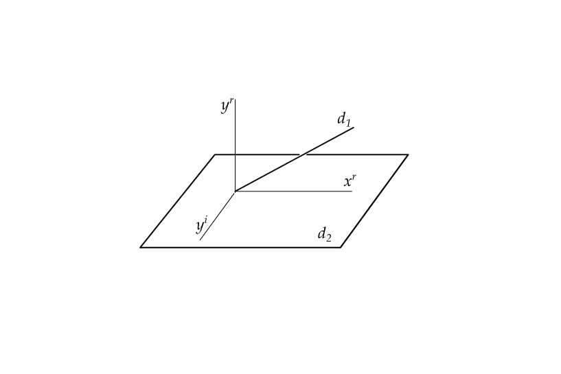
Figure 1: representation of the branes worldvolumes and the spacetime coordinates (note that coordinates $x^{\rho}$ and $z^{a}$ can not be displayed in this figure)

We choose $x^{\alpha}:=(x^{\rho},x^{r})$ as the parameterizing coordinates of the probe and $y^{A}:=(y^{i},y^{r},z^{a})$ as its embedding coordinates. According to the count of coordinates in table (1), there are cases for which some of the coordinates in our decompoition are not present. For example, when $d_{1}=d_{2}$, we have no $y^{i}$ coordinates. Similarly, when $d_{1}=\delta$ (i.e., the two branes are parallel), there are no $x^{r}$ and $y^{r}$ coordinates. However, this has no effect on our general equations as they are formulated in terms of the coordinates $x^{\alpha}$ and $y^{A}$ regardless their numbers.

Thus, the embedding coordinates for a probe rotated/boosted relative to a fixed source are represented as

$$Y^{A}(x)={\omega}^{A}_{\alpha}x^{\alpha}+y^{A}_{0}$$ (1)

with $\omega$’s and $y_{0}$’s representing constant slopes/velocities and shifts. It is clear from the definitions in table (1) that

$${\omega}^{A}_{\rho}={\omega}^{i}_{\alpha}={\omega}^{a}_{\alpha}=0$$ (2)

That is, $(Y^{i},Z^{a})$ are constants and none of $Y^{A}$’s depend on $(x^{\rho})$. Evidently, the remaining ${\omega}$’s can not have arbitrary values. In fact, they have to be chosen in a way that eq.(1) solves the $(d_{1}-1)$-brane equations of motion:

$${\partial}_{\alpha}\left({{\partial{\cal L}}\over{\partial Y^{A}_{,\alpha}}}\right)-{{\partial{\cal L}}\over{\partial Y^{A}}}=0$$ (3)

where ${\cal L}(Y^{A},{\partial}_{\alpha}Y^{A})$ denotes the relevant worldvolume Lagrangian. That is, $\omega$’s must be such the identities

$${{\partial}\over{\partial Y^{B}}}\left({\omega}^{B}_{\alpha}{{\partial{\cal L}}\over{\partial{\omega}^{A}_{\alpha}}}-{\delta}^{B}_{A}{\cal L}\right)\equiv 0$$ (4)

hold for all values of $(x^{r})$. Here, ${\cal L}$ have to be considered as the function ${\cal L}(Y^{A};{\omega}^{A}_{\alpha})$, whose $Y^{A}$-dependences turn to appear in the form

$${\cal L}(Y^{A};{\omega}^{A}_{\alpha})={\cal L}\left(H(\sqrt{(Y^{r})^{2}+(Z^{a})^{2}})\ ;\ {\omega}^{A}_{\alpha}\right)$$ (5)

where $H$ represents a harmonic function in the $(y^{r},z^{a})$-directions [16]. Taking this into account, and that $Y^{r}$’s are independent coordinates as far as $x^{r}$’s are so, one can see that eq.(4) leads to

$${{\partial{\cal L}}\over{\partial H}}Z^{a}=0$$ (6)

$${{\partial}\over{\partial H}}\left({\omega}^{r}_{\alpha}{{\partial{\cal L}}\over{\partial{\omega}^{s}_{\alpha}}}-{\delta}^{r}_{s}{\cal L}\right)=0$$ (7)

We will refer to eqs.(6),(7) as the ‘no-force’ and ‘no-torque’ conditions, respectively, since they are indeed the conditions for the vanishing of the oscillations along the transverse directions of the two branes, as well as their (relative) rotations along the relative transverse directions (see section 7).

2.1 The marginal and non-marginal configurations

By definition, a ‘marginal’ configuration of two branes is the one which is stable at any arbitrary separations of the two branes, i.e., for any constant values of $Z^{a}$’s. This, according to eq.(6), implies

$${\cal L}(H;\omega)\equiv{{\cal L}}_{0}(\omega)$$ (8)

showing that the total potential energy between the two branes has a constant value. It is obvious that eq.(7) in this case is automatic and hence the above equation is the unique description of the ‘marginal’ configurations.

There exist other configurations, however, that can be formed only at zero separations of the two participating branes, i.e., when the centers of the two branes in their transverse space are coincident and they actually intersect each other. We refer to these as the non-marginal configurations [17]. For such solutions, with $Z^{a}=0$, eq.(6) is automatic and hence eq.(7) or its equivalent as

$${\omega}^{r}_{\alpha}{{\partial{\cal L}}\over{\partial{\omega}^{s}_{\alpha}}}-{\delta}^{r}_{s}{\cal L}\equiv{{\cal C}}^{r}_{s}(\omega)$$ (9)

provides a unique description for the non-marginal configurations. In the following three sections, we analyze the eqs.(8),(9) for classifying several marginal and non-marginal configurations that may occur in cases with a pair of similar $(d_{1}=d_{2})$, non-similar $(d_{1}\neq d_{2})$ and electromagnetic dual $(d_{1}={{\tilde{d}}}_{2})$ branes. The notations will be mainly identical to those introduced in [14, 16].

3 Configurations with similar branes

Using the general expression of the Lagrangian for a $(d-1)$-probe in a $(d-1)$-source background [16], the function ${\cal L}(H;\omega)$ is found to be

$${\cal L}=H^{-1}[det^{1/2}({\bf 1}+H{\bf\Theta})-1]$$ (10)

where the angular information is encoded in the matrix ${\bf\Theta}$ having the components

$${\Theta}^{\alpha}_{\beta}:={\omega}^{r\alpha}{\omega}^{r}_{\beta}$$ (11)

and the indices of the type of $\alpha$ are raised and lowered by ${\eta}_{\alpha\beta}:=diag(-1,+1,\cdot\cdot\cdot,+1)$. The matrix ${\bf\Theta}$ can be diagonalized by choosing the coordinates $(x^{r},y^{r})$ so that the two branes to be related by a set of ‘commuting’ rotations and a boost. In such coordinates, ${\bf\Theta}$ has the components

$${\Theta}^{\alpha}_{\beta}=diag(-v^{2},tan^{2}{\theta}_{1},\cdot\cdot\cdot,tan^{2}{\theta}_{d-1})=:{\delta}^{\alpha}_{\beta}{\Theta}_{\alpha}$$ (12)

Here, $v$ represents the magnitude of the velocity vector in the directions transverse to the $(d-1)$-source and $\theta$’s are the angles of the $(d-1)$ commuting rotations (obviously, a number $\delta$ of these angles are vanishing by assumption).

3.1 Marginal intersections

Inserting the expression (10) for ${\cal L}$ into the ‘marginality’ condition, eq.(8), one obtains

$$det({\bf 1}+H{\bf\Theta})\equiv(1+{{\cal L}}_{0}H)^{2}\ \ \ \ \ (\forall H>0)$$ (13)

In the basis that ${\bf\Theta}$ has the form of eq.(12), this identity reads

$$(1-v^{2}H)(1+tan^{2}{\theta}_{1}H)\cdot\cdot\cdot(1+tan^{2}{\theta}_{d-1}H)\equiv(1+{{\cal L}}_{0}H)^{2}$$ (14)

Thus the only possibility for the rotation and boost parameters is

$${\theta}_{1}=\pm{\theta}_{2}=:\theta$$

$$v={\theta}_{3}=\cdot\cdot\cdot={\theta}_{d-1}=0$$ (15)

That is:
the only marginal configuration of two similar branes are the static configurations with two non-vanishing angles obtained by an abelian subgroup of the $SU(2)$ rotations.
This is the same as the 1/4 SUSY configuration whose supergravity solution had been found earlier in [14] as a generalization to the solution of 2-branes at angles [7]. The constant value of ${\cal L}$ in this case is ${{\cal L}}_{0}=tan^{2}\theta$.
Another possibility, which one might consider for two similar branes, was the brane-anti-brane system. In this case the constant term $(-1)$ in brackets in eq.(10) would be flipped to (+1) which is equivalent to flipping ${{\cal L}}_{0}$ to $-{{\cal L}}_{0}$ in eq.(13) or (14). However, because ${{\cal L}}_{0}\geq 1$ in this case, eq.(14) could not be satisfied for any real values of $v$ and $\theta$’s. In other words, a brane-anti-brane pair with any combination of a boost and several rotations is unstable and can not form a marginal configuration.

3.2 Non-marginal configurations

It is easy to see that the ‘non-marginality’ condition, eq.(9), after some algebra reduces to

$$\sqrt{\Omega}({\bf\Omega}^{-1})^{\alpha\beta}{\omega}^{r}_{\alpha}{\omega}^{s}_{\beta}-{\delta}^{rs}H^{-1}(\sqrt{\Omega}-1)={{\cal C}}^{rs}$$ (16)

where ${\bf\Omega}:={{\bf 1}}+H{\bf\Theta}$ , $\Omega:=det\bf\Omega$ and $({{\cal C}}^{rs})$ are a set of angle-dependent constants. In the basis that makes ${\bf\Theta}$ diagonal (eq.(12)), the above equation is also diagonal and after some manipulations yields

$$\prod_{\alpha}(1+H{\Theta}_{\alpha})\equiv(1+H{\Theta}_{r})^{2}(1+H{{\cal C}}_{r})^{2}\ \ \ \ \ \ (\forall H>0)$$ (17)

where ${{\cal C}}^{rs}=:{\delta}^{rs}{{\cal C}}_{r}$. For this equation to be satisfied identically, one needs

$${\theta}_{1}=\pm{\theta}_{3}\ ,\ {\theta}_{2}=\pm{\theta}_{4}$$

$$v={\theta}_{5}=\cdot\cdot\cdot={\theta}_{d-1}=0$$ (18)

That is:
the only ‘non-marginal’ configurations of two ‘similar’ branes are the static configurations with four angles obtained by two independent abelian subgroup of the $SU(2)$ rotations.

It is easy to check that, unless one of the $({\theta}_{1},{\theta}_{2})$ vanishes, in this case ${\cal L}$ is not a constant, but it is a linear function of $H$. Orthogonal configurations of the 4-angle intersections have been found previously in the literature of the supergravity composite brane solutions [21]. The most famous examples in this category consist of the $NS5\cap NS5=1$ in $D=10$ II A,B , $D5\cap D5=1$ in $D=10$ II B and $M5\cap M5=1$ in D=11 [21]. In a recent paper [8], a 4-angle configuration of this type for the II A NS5-branes at Sp(2) angles has been found, by directly solving the supergravity and Killing spinor equations, showing that it preserves at least 3/32 of the SUSY (see however [9, 2, 1, 5]).

4 Configurations of two non-similar branes

The general worldvolume Lagrangian for a $(d_{1}-1)$-probe in a $(d_{2}-1)$-source background, with $d_{1}<d_{2}$ [16], gives rise to an expression for ${\cal L}(H;\omega)$ as

$${\cal L}=H^{-m/2}det^{1/2}({\bf 1}+H{\bf\Theta})$$ (19)

where ${\bf\Theta}$ is given by eq.(11) and $m$ is a function of dimensions defined as

$$m(d_{1},d_{2}):=2\alpha(d_{1})\alpha(d_{2})+{{d_{1}{{\tilde{d}}}_{2}}\over{D-2}}$$ (20)

For marginal configurations, $m$ specifies the number of (non-vanishing) angles (see [14] and below). Here, $\alpha(d)$ represents the dilaton-d-form coupling constant satisfying [18]

$${\alpha}^{2}(d)=1-{{d{\tilde{d}}}\over{2(D-2)}}$$ (21)

4.1 Marginal intersections

The marginality condition, eq.(8), in this case gives

$$\prod_{\alpha}(1+H{\Theta}_{\alpha})\equiv{{\cal L}}_{0}^{2}H^{m}\ \ \ \ \ \ \ (\forall H>0)$$ (22)

Obviously, such an identity can be true whenever $m\in{\bf Z}^{+}$, and a number $m$ of ${\Theta}_{\alpha}$’s to be $+\infty$, while the remaining are vanishing. This implies that

$${\theta}_{1}=\cdot\cdot\cdot={\theta}_{m}=\pi/2$$

$${\theta}_{m+1}=\cdot\cdot\cdot={\theta}_{d_{1}-1}=v=0$$ (23)

The number of common directions then is $\delta=d_{1}-m$. Therefore:
the only ‘marginal’ bound state of a pair of ‘non-similar’ $(d_{1}-1,d_{2}-1)$-branes are the ‘static orthogonal’ configurations in which the two branes share $(\delta-1)$ of their directions, where $\delta$ must satisfy

$$\delta=-2\alpha(d_{1})\alpha(d_{2})+{{d_{1}d_{2}}\over{D-2}}$$ (24)

This is, in fact, the so called ‘intersection rule’ of the intersecting brane systems, which was originally found in the study of their supergravity solutions [19, 20], and then re-appeared in the reduced Lagrangian approach to the distributed brane systems in [14] and was interpreted there as an algebraic constraint required by the no-force conditions [23].

4.2 Non-marginal Intersections

The ‘non-marginality’ condition, eq.(9), in this case gives the counterpart of eq.(16) as

$$H^{-m/2}\sqrt{\Omega}\{H({\bf\Omega}^{-1})^{\alpha\beta}{\omega}^{r}_{\alpha}{\omega}^{s}_{\beta}-{\delta}^{rs}\}={{\cal C}}^{rs}$$ (25)

which in the ${\bf\Theta}$-diagonalizing basis (eq.(12)) takes the form of the identity

$$\prod_{\alpha}(1+H{\Theta}_{a})\equiv{{\cal C}}_{r}^{2}H^{m}(1+H{\Theta}_{r})^{2}\ \ \ \ \ \ \ \ \ (\forall H>0)$$ (26)

which is the analogue of eq.(17). Obviously, such an identity holds (for each $r$), if and only if $m\in{\bf Z}^{+}$, and further $(m+2)$ of ${\Theta}_{\alpha}$’s are infinity while the others are vanishing. Therefore,

$${\theta}_{1}=\cdot\cdot\cdot={\theta}_{m+2}=\pi/2$$

$${\theta}_{m+3}=\cdot\cdot\cdot={\theta}_{d_{1}-1}=v=0$$ (27)

These are just the conditions (23) in which $m$ has been replaced by $(m+2)$. So we have the result:
the only ‘non-marginal’ bound state of a pair of ‘non-similar’ $(d_{1}-1,d_{2}-1)$-branes are the ‘static orthogonal’ configurations in which the two branes share $(\delta-1)$ of their directions, with $\delta$ satisfying

$$\delta+2=-2\alpha(d_{1})\alpha(d_{2})+{{d_{1}d_{2}}\over{D-2}}$$ (28)

which shifts $\delta$ by a $-2$ relative to the one given by the rule (24). This is just the same equation identified as the intersection rule of the ‘localized intersections’ in [21]. By the above derivation, however, it has to be identified as a rule for the ‘non-marginal’ intersections.

5 Configurations with an electromagnetic dual pair of branes

An ‘electromagnetic’ dual pair of branes, a priori, can not be placed in either of the two categories studied in sections 3,4. This is due to the fact that an electromagnetic dual pair with $(d-1,{\tilde{d}}-1)$-branes is the source of a single $d$-form potential ${{\cal A}}_{(d)}$, which couples to the two branes through ${{\cal F}}_{(d+1)}=d{{\cal A}}_{(d)}$ and its dual ${}^{*}{{\cal F}}_{(d+1)}$ respectively [18]. Taking this point into account, and assuming $d\leq{\tilde{d}}$ to adapt with the conventions of section 2, one obtains the modified version of eq.(4) as

$${{\partial}\over{\partial Y^{n}}}\left({\omega}^{n}_{\alpha}{{\partial{\cal L}}\over{\partial{\omega}^{m}_{\alpha}}}-{\delta}_{mn}{\cal L}-{\gamma}_{mn}H\right)\equiv 0$$ (29)

where ${\cal L}$ is defined in eq.(19) in which $m=d-2$, and the constants ${\gamma}_{mn}$ are defined as

$${\gamma}_{mn}:={\epsilon}_{mnl_{1}\cdot\cdot\cdot l_{d}}{\epsilon}^{{\alpha}_{1}\cdot\cdot\cdot{\alpha}_{d}}{\omega}^{l_{1}}_{{\alpha}_{1}}\cdot\cdot\cdot{\omega}^{l_{d}}_{{\alpha}_{d}}/(d!)^{2}$$ (30)

Here, the two epsilons stand for the Levi-Civita symbols in the subspaces of $(y^{m}):=(y^{r},z^{a})$ and $(x^{\alpha})$, respectively. The modifying term ${\gamma}_{mn}H$ in eq.(29), however, does not modify the results of section 4 for the branes at angles with $(d_{1},d_{2})=(d,{\tilde{d}})$. The reason, as can be checked using eq.(12), is that in all $\delta\geq 1$ cases one obtains ${\gamma}_{mn}=0$. Thus the rule (24) (with $\alpha(d)=-\alpha({\tilde{d}})$) and eq.(21) imply $\delta=2$. Hence:
the only marginal configuration of an electromagnetic dual pair of $(d-1,{\tilde{d}}-1)$-branes is a ‘static’ configuration in which the two branes ‘orthogonally’ intersect (overlap) on a string.

On the other hand, a non-marginal configuration should obey the rule (28), which in this case implies that $\delta=0$. This is in obvious contradiction with the static-ness property asserted above the rule (28) which means that such configurations of $(d,{\tilde{d}})$ can not be realized.

5.1 Non-marginal configuration of parallel branes

The results of the previous sections regarding the non-marginal configurations , in particular their intersection rule (eq.(28)), are based on the no-torque condition (eq.(7)) which severly relies on the existence of at least one pair of coordinates $(x^{r},y^{r})$ in table (1). Since for a pair of parallel branes (i.e. a configuration of the form $d_{1}\subseteq d_{2}$) there are no such coordinates, hence the stability condition for such configurations should have a different form. Whatever the form of these conditons, they should guarantee that the equations of motion (eq.(4)) are satisfied. In the case at hand all ${\omega}^{A}_{\alpha}$’s are zero and this equation reduces to: $\partial{\cal L}/\partial Y^{A}=0$, where ${\cal L}(Y^{A})$ is the same as ${\cal L}\left(H(Y^{A});{\omega}^{A}_{\alpha}=0\right)$. Noting that $H$ in this case depends only on $Z^{a}$ through $r:=\sqrt{Z^{a}Z^{a}}$, and further that $Z^{a}=0$ in the non-marginal case, the above equation yields:

$${{\partial V(r)}\over{\partial r}}\large|_{r=0}=0$$ (31)

where $V(r):={\cal L}\left(H(r);{\omega}^{A}_{\alpha}=0\right)$. For a pair of non-similar branes we find from eq.(19) that

$$V(r)=(H(r))^{-m/2}=\left(1+{{Q_{2}}\over{r^{M-2}}}\right)^{-m/2}$$ (32)

Here $M:=\tilde{d}_{2}+2$ is the transverse dimension and $Q_{2}$ is (proportional to) the charge of $(d_{2}-1)$-brane and $m$ is defined as in eq.(20). (We have assumed that $d_{1}\leq d_{2}$ and $\tilde{d}_{2}>0$.) It is obvious that $V(r)$ is proportional to the potential energy between the two branes at a separation $r$ and eq.(31) indicates that their mutual forces tend to balance each other as $r\rightarrow 0$. Now, since in this limit $V(r)\sim r^{m(M-2)/2}$, the above condition means that the function $V(r)$ should be regular near $r=0$ at least to the first order in its derivatives, requiring that

$$m(M-2)>2$$ (33)

or equivalently

$${\alpha}_{1}{\alpha}_{2}>{{2(D-2)-d_{1}\tilde{d}_{2}^{2}}\over{2\tilde{d}_{2}(D-2)}}$$ (34)

This inequality together with $d_{1}\leq d_{2}$ and $\tilde{d}_{2}>0$ in turn specifies all the non-marginal bound states of the form of branes within branes. Special cases of such configurations are those with a self dual pair, i.e. with $d_{1}=d\ ,\ d_{2}=\tilde{d}$. Since in this case $M=d+2$ , $m=d-2$, the above condition (assuming $d\leq\tilde{d}$) yields: $3\leq d\leq(D-2)/2$ showing that such configurations are possible only in $D\geq 8$ dimensions. Famous examples of such configurations are $M2\subset M5$ in $D=11$ and the dyonic membrane (bound state of an electric and a magnetic 2-brane) in $D=8$ dimensions, which were known through their supergravity solutions [22].

6 Multi-angle marginal intersections

The results of the previous sections indicate that, except for the 2-angle static configuration of similar branes at $SU(2)$ angles, no other configuration of two flat branes with several angles and boost can be marginally stable. While, both the scattering amplitude and superalgebra computations [5, 2] indicate that multi-angle intersections, under certain conditions among their angles, can form a marginal configuration, it is amazing that the worldvolume solutions appropriate to a pair of flat branes are not realizable. This apparent contradiction is resolved by recalling that all the scattering amplitude and superalgebra computations rely heavily on the basic assumption for the existence of an ‘asymptotic state’ in which the branes behave like flat hypersurfaces in a Minkowski space. In the string theory language, the perturbative calculation of the scattering amplitudes are reliable only in the weak coupling region of the theory where one deals with weak (linearized) gravitational interactions. This restricts such calculations to the ‘far’ or ‘asymptotic’ region of the two branes where they look like flat hypersurfaces in a flat spacetime. On the SUSY side, also, one does not need to solve a Killing spinor equation in all of the space to determine SUSY fraction preserved by a brane configuration. To do this, it suffices to solve only the asymptotic (algebraic) Killing spinor equation [3, 2, 1], which encodes only the asymptotic form of the spacetime metric and of the geometry of branes. As a result, there may be BPS states of curved p-branes which look like asymptotically as multi-angle configurations of flat p-branes. In the asymptotic region, we will see that the no-force condition to first order will require a certain angular constraint which is just the same that characterizes these BPS states [5, 6]. However, the same no-force condition to higher orders, as well as the no-torque condition, are not satisfied except for the marginal configurations which were categorized in sections 3,4. This means, firstly, that the marginal multi-angle configurations, generally, can not consist of flat p-branes. Secondly, even in the case of an asymptotically force-free configuration, the relative angular position of the two branes is influenced by a non-vanishing torque which eventually brings them together by counterbalancing the forces that act between themselves. In general, the force and torque conditions, eq.(8),(9), are equivalent to a set of algebraic constraints relating ${\Theta}^{\alpha}_{\beta}$’s together. This can be seen easily by putting $H:=1+h$ and expanding ${\cal L}(H;\omega)$ as

$${\cal L}(1+h;\omega)=\sum_{n=0}^{\infty}{{1}\over{n!}}{{\cal L}}_{n}(\omega)h^{n}$$ (35)

Upon this expansion, eqs.(8),(9) give respectively

$${{\cal L}}_{n}(\omega)=0$$ (36)

$${\omega}^{r}_{\alpha}{{\partial{{\cal L}}_{n}}\over{\partial{\omega}^{s}_{\alpha}}}-{\delta}^{r}_{s}{{\cal L}}_{n}=0$$ (37)

where $n=1,2,\cdot\cdot\cdot$ . For a ‘real’ marginal bound state of flat p-branes, these two sets of equations for all $n$ restrict possible configurations to those of sections 3,4. However, for a configuration of curved p-branes with asymptotic flat geometries, we may continue to define the marginality property by demanding that ${\cal L}(H;\omega)$ to be constant only to first order in $(H-1)$ in the asymptotic region $H(y)\rightarrow 1$. Such ‘asymptotic marginal’ configurations, thus, are distinguished by a condition on the angles as ${{\cal L}}_{1}(\omega)=0$. This condition, though provides a mean of translational stability, does not insure rotational stability of the two brane system, which to be guaranteed by the eq.(37) for $n=1$. These two conditions together, will be seen that, restrict the possible marginal configurations to those obtained in sections 3,4. We now examine the explicit expressions of these conditions in the previous cases.

6.1 Similar branes

It is easy to see, by expanding eq.(10) to ${\cal O}(h)$, that in this case

$${{\cal L}}_{0}(\Theta)=det^{1/2}({\bf 1}+{\bf\Theta})-1$$

$${{\cal L}}_{1}(\Theta)=det^{1/2}({\bf 1}+{\bf\Theta})\left\{{1\over 2}Tr\left({{{\bf\Theta}}\over{{\bf 1}+{\bf\Theta}}}\right)-1\right\}+1$$ (38)

where $\omega$ dependences are encoded in ${\bf\Theta}$ as is defined in eq.(11). (The expression for ${{\cal L}}_{0}$ is given only for later reference.) Diagonalizing ${\bf\Theta}$ as in eq.(12), the ${{\cal L}}_{1}=0$ equation becomes

$$F(\theta):=\prod_{\alpha=0}^{d-1}cos{\theta}_{\alpha}+{1\over 2}\sum_{\alpha=0}^{d-1}sin^{2}{\theta}_{\alpha}-1=0$$ (39)

where, for convenience, we have included the velocity $v$ in $\theta$’s by defining ${\theta}_{0}:=tan^{-1}(iv)$. Solving eq.(39) for $v$, however, shows that combinations of boost and rotations for less than three non-vanishing angles do not define allowable configurations. Indeed, one can see using eq.(39), that the one- and two-angle configurations are limited only to the parallel and $SU(2)$-rotated static configurations respectively. If, in addition to the above condition, one requires rotational stability of the configuration, eq.(37) for $n=1$ gives

$${{\partial F}\over{\partial{\theta}_{\alpha}}}=sin{\theta}_{\alpha}\left(\prod_{\beta\neq\alpha}cos{\theta}_{\beta}-cos{\theta}_{\alpha}\right)=0$$ (40)

The only simultaneous solutions of eqs.(39),(40), when more than two ${\theta}_{\alpha}$’s exist, are the one with

$${\theta}_{1}={\theta}_{2}\ \ ,\ \ {\theta}_{0}={\theta}_{3}=\cdot\cdot\cdot={\theta}_{d-1}=0$$ (41)

and its permutations for ${\theta}_{\alpha}$’s ($\alpha\neq 0$). That is, the only rotationally stable marginal configurations are those with $SU(2)$ angles.

6.2 Non-similar branes

In this case eq.(19) gives

$${{\cal L}}_{0}(\Theta)=det^{1/2}({\bf 1}+{\bf\Theta})$$

$${{\cal L}}_{1}(\Theta)={1\over 2}det^{1/2}({\bf 1}+{\bf\Theta})\left\{Tr\left({{{\bf\Theta}}\over{{\bf 1}+{\bf\Theta}}}\right)-m\right\}$$ (42)

So, in the basis of eq.(12), the ${{\cal L}}_{1}=0$ condition becomes

$$F(\theta):=\sum_{\alpha=0}^{d_{1}-1}sin^{2}{\theta}_{\alpha}-m=0\ \ \ \Rightarrow$$

$$-2\alpha(d_{1})\alpha(d_{2})+{{d_{1}d_{2}}\over{D-2}}=\sum_{\alpha=0}^{d_{1}-1}cos^{2}{\theta}_{\alpha}$$ (43)

This gives, in fact, a modification of the usual intersection rule, eq.(24), to the general case involving arbitrary boost and angles between the two branes. Obviously, an ‘orthogonal static’ limit, with ${\theta}_{\alpha}$’s equal to $0,\pi/2$, exists only in cases with $m\in{\bf Z}^{+}$. That is, for an orthogonal intersection, the rule (24) must hold and in such a case $m$ counts the number of ${\theta}_{\alpha}=\pi/2$ angles. Despite eq.(39), the eq.(43) allows for the possibility of the combinations of a boost with any number of angles. Specially, when $m\leq 0$, one can find (asymptotically) boosted configurations of two parallel branes having a relative velocity $v=\sqrt{{m\over{m-1}}}$. However, configurations defined by eq.(43) are not rotationally stable, unless we have

$${{\partial F}\over{\partial{\theta}_{\alpha}}}=2sin{\theta}_{\alpha}cos{\theta}_{\alpha}=0$$ (44)

which means that ${\theta}_{\alpha}$’s must be $0,\pi/2$. Therefore, the rotationally stable marginal configurations are the static ones with orthogonal branes obeying the rule (24).

7 Small perturbations on the worldvolume

So far, we have stressed on the fact that every ‘equilibrium’ configuration of two flat p-branes is specified by the two requirements, eqs.(6),(7), which we have interpreted as the no-force and no-torque conditions respectively. In this section, we try to make this correspondences explicit by perturbing the worldvolume of one of the branes (the probe) with respect to its flat state, while the other brane (the source) is kept flat and fixed. This type of description is similar to the one which is used in [16]. To be concrete, we first present a perturbative formulation of the classical solutions for a general field theory with one expansion parameter, and then consider its application to the worldvolume field theory of the probe.

7.1 General field theory formulation

Assume that a field theory, for the variable(s) $\phi(x)$, is defined by means of the perturbative Lagrangian

$${\cal L}[\phi;\varepsilon]={{\cal L}}_{0}[\phi]+\varepsilon{{\cal L}}_{1}[\phi]+{{{\varepsilon}^{2}}\over 2}{{\cal L}}_{2}[\phi]+\cdot\cdot\cdot$$ (45)

with $\varepsilon$ being the perturbation parameter. Now, take ${\phi}_{0}(x)$ to represent a classical solution of the unperturbed Lagrangian ${{\cal L}}_{0}[\phi]$, i.e., it satisfies the equation of motion: ${{\delta{{\cal L}}_{0}}\over{\delta\phi}}=0$. The question, which we like to answer, is that how can we specify a solution of the perturbed Lagrangian which tends to ${\phi}_{0}(x)$ when $\varepsilon\rightarrow 0$. Obviously, such a solution must obey the expansion

$$\phi(x;\varepsilon)={\phi}_{0}(x)+\varepsilon{\phi}_{1}(x)+{{{\varepsilon}^{2}}\over 2}{\phi}_{2}(x)+\cdot\cdot\cdot$$ (46)

Putting this expansion in eq.(45), and using the functional Taylor series expansion of ${{\cal L}}_{n}$’s, the overall expansion of ${\cal L}[\phi(x;\varepsilon);\varepsilon]$ in powers of $\varepsilon$ takes the form

$${\cal L}[{\phi}_{0},{\phi}_{1},\cdot\cdot\cdot;\varepsilon]={{\cal L}}_{0}[{\phi}_{0}]+\varepsilon\left({{\delta{{\cal L}}_{0}}\over{\delta\phi}}{\phi}_{1}+{{\cal L}}_{1}\right)+{{{\varepsilon}^{2}}\over 2}\left({{\delta{{\cal L}}_{0}}\over{\delta\phi}}{\phi}_{2}+{{{\delta}^{2}{{\cal L}}_{0}}\over{\delta{\phi}^{2}}}{\phi}_{1}^{2}+2{{\delta{{\cal L}}_{1}}\over{\delta\phi}}{\phi}_{1}+{{\cal L}}_{2}\right)+\cdot\cdot\cdot$$ (47)

where all ${{\cal L}}_{n}$’s and their functional derivatives are evaluated at $\phi={\phi}_{0}$. Treating $\{{\phi}_{n}\}$ as a set of independent variables, and varying ${\cal L}$ with respect to these variables, one picks the set of equations

$${{\delta{{\cal L}}_{0}}\over{\delta\phi}}=0$$

$${{{\delta}^{2}{{\cal L}}_{0}}\over{\delta{\phi}^{2}}}{\phi}_{1}+{{\delta{{\cal L}}_{1}}\over{\delta\phi}}=0$$

$${{{\delta}^{2}{{\cal L}}_{0}}\over{\delta{\phi}^{2}}}{\phi}_{2}+{{{\delta}^{3}{{\cal L}}_{0}}\over{\delta{\phi}^{3}}}{\phi}_{1}^{2}+2{{{\delta}^{2}{{\cal L}}_{1}}\over{\delta{\phi}^{2}}}{\phi}_{1}+{{\delta{{\cal L}}_{2}}\over{\delta\phi}}=0\ ,\ etc.$$ (48)

These equations, in principle , determine the solutions for ${\phi}_{0}(x),\ {\phi}_{1}(x),\ etc.$ in the successive order. It is worth-pointing that, except for ${\phi}_{0}(x)$ which is assumed to be a given solution of ${{\cal L}}_{0}$, all other ${\phi}_{n}$’s are determined by solving a linear inhomogeneous PDE of the form

$${{{\delta}^{2}{{\cal L}}_{0}}\over{\delta{\phi}^{2}}}{\phi}_{n}={{\cal J}}_{n}$$ (49)

where the source term ${{\cal J}}_{n}(x)$ in the $n$-th stage is a known function of $x$, constructed from ${\phi}_{0}(x),\cdot\cdot\cdot,{\phi}_{n-1}(x)$. For vanishing boundary conditions on ${\phi}_{n}$’s, one solves eq.(49) symbolically as ${\phi}_{n}=G{{\cal J}}_{n}$, with $G$ representing the Green’s function of the linear operator ${{{\delta}^{2}{{\cal L}}_{0}}\over{\delta{\phi}^{2}}}$ at $\phi={\phi}_{0}$. If ${{\cal L}}_{0}$, as in usual, is a first order Lagrangian in terms of the $\phi$-derivatives, then ${{{\delta}^{2}{{\cal L}}_{0}}\over{\delta{\phi}^{2}}}$ will be a second order linear differential operator with (in general) spacetime dependent coefficients, whose Green’s function is constructed in the usual manner. The above procedure, thus eventually, determines $\phi(x;\varepsilon)$ to any arbitrary order in the expansion parameter $\varepsilon$.

7.2 Application to the worldvolume field theory

We consider a source-probe configuration of arbitrary branes, as in [16], and choose the embedding of the probe, as in section 2, to be represented by $Y^{A}=Y^{A}(x^{\alpha})$. It is clear that the worldvolume Lagrangian of the probe has a generic form as

$${\cal L}[Y]={\cal L}\left(h(Y^{A}),{\partial}_{\alpha}Y^{A}\right)$$ (50)

where the explicit dependences on $Y^{A}$ are encoded in the harmonic function $h$ of the transverse distance from the source, which is proportional to its charge or tension $T_{s}$, and vanishes asymptotically. Obviously, taking the limit $T_{s}\rightarrow 0$ is equivalent to going to the asymptotic region of $Y^{A}$, where the source and probe have a large separation, and in this limit eq.(50) takes the form of an ordinary Lagrangian of a minimal surface in the Minkowski space. Taking this as the unperturbed Lagrangian ${{\cal L}}_{0}$, and treating $T_{s}$ as a perturbation parameter, the perturbed Lagrangian ${\cal L}$ will be expanded as

$${\cal L}[Y]=\sum_{n=0}^{\infty}{1\over{n!}}h^{n}(Y){{\cal L}}_{n}(\partial Y)$$ (51)

which is nothing but the eq.(35) with ${\omega}^{A}_{\alpha}$’s replaced by ${\partial}_{\alpha}Y^{A}$’s. Also, it is clear that ${{\cal L}}_{0}$ has classical solutions which are in the form of flat hypersurfaces, similar to the one in eq.(1), which plays here the role of the ‘unperturbed solution’ $Y^{A}_{0}(x)$. The main advantage of this choice for $Y^{A}_{0}(x)$ is that it renders ${{\cal L}}_{n}[Y_{0}]$’s as constant parameters ${{\cal L}}_{n}(\omega)$. This means that we are interested in a probe whose worldvolume geometry, in the region far from the source, is that of a flat hypersurfaces, though it may be curved in the near region. Thus, perturbing the flat solutions as $Y^{A}(x)=Y^{A}_{0}(x)+Y^{A}_{1}(x)+\cdot\cdot\cdot$, and using the general formulation of the previous subsection, one finds that the first order perturbation, $Y^{A}_{1}(x)$, obeys the equation

$${{{\partial}^{2}{{\cal L}}_{0}}\over{\partial{\omega}^{A}_{\alpha}\partial{\omega}^{B}_{\beta}}}{\partial}_{\alpha}{\partial}_{\beta}Y^{B}_{1}+\left({\omega}^{A}_{\alpha}{{\partial{{\cal L}}_{1}}\over{\partial{\omega}^{B}_{\alpha}}}-{\delta}_{AB}{{\cal L}}_{1}\right){\partial}_{B}h(Y_{0})=0$$ (52)

The eq.(52) represents a system of second order PDE with the constant coefficients ${{{\partial}^{2}{{\cal L}}_{0}}\over{\partial{\omega}^{A}_{\alpha}\partial{\omega}^{B}_{\beta}}}$ and source terms which are linear combinations of ${\partial}_{B}h(Y_{0}(x))$. Now, using the expression (38) or (42) for ${{\cal L}}_{0}(\Theta)$, one can show that

$${{{\partial}^{2}{{\cal L}}_{0}}\over{\partial{\omega}^{A}_{\alpha}{\omega}^{B}_{\beta}}}={{\cal L}}_{0}\{{\delta}^{AB}{\Omega}^{\alpha\beta}+{\omega}^{A}_{\gamma}{\omega}^{B}_{\delta}({\Omega}^{\alpha\gamma}{\Omega}^{\beta\delta}-{\Omega}^{\beta\gamma}{\Omega}^{\alpha\delta}-{\Omega}^{\alpha\beta}{\Omega}^{\gamma\delta})\}$$ (53)

where ${\Omega}^{\alpha}_{\ \beta}:=[({\bf 1}+{\bf\Theta})^{-1}]^{\alpha}_{\ \beta}$. Inserting this into the eq.(52), we obtain

$$I_{AB}{\Omega}^{\alpha\beta}{\partial}_{\alpha}{\partial}_{\beta}Y^{B}_{1}+{1\over{{{\cal L}}_{0}}}\left({\omega}^{A}_{\alpha}{{\partial{{\cal L}}_{1}}\over{\partial{\omega}^{B}_{\alpha}}}-{\delta}^{AB}{{\cal L}}_{1}\right){\partial}_{B}h(Y_{0})=0$$ (54)

where $I_{AB}:={\delta}_{AB}-{\Omega}^{\gamma\delta}{\omega}^{A}_{\gamma}{\omega}^{B}_{\delta}$. It is easy to see, using eq.(2), that the above equation for $A=i,a,r$ (as defined in table (1)) is decomposed into the three uncoupled equations

$${\Omega}^{a\beta}{\partial}_{\alpha}{\partial}_{\beta}Y^{i}_{1}=0$$ (55)

$${\Omega}^{a\beta}{\partial}_{\alpha}{\partial}_{\beta}Z^{a}_{1}-{{{{\cal L}}_{1}}\over{{{\cal L}}_{0}}}{\partial}_{a}h(Y_{0})=0$$ (56)

$$I_{rs}{\Omega}^{a\beta}{\partial}_{\alpha}{\partial}_{\beta}Y^{s}_{1}+{1\over{{{\cal L}}_{0}}}\left({\omega}^{r}_{\alpha}{{\partial{{\cal L}}_{1}}\over{\partial{\omega}^{s}_{\alpha}}}-{\delta}_{rs}{{\cal L}}_{1}\right){\partial}_{s}h(Y_{0})=0$$ (57)

where we have used the fact that ${\partial}_{i}h=0$. The operator ${\Omega}^{a\beta}{\partial}_{\alpha}{\partial}_{\beta}$ appearing above is indeed the D’ Alembertian operator along the probe’s worldvolume coordinates, as can be seen by the eq.(12),

$${\Omega}^{a\beta}{\partial}_{\alpha}{\partial}_{\beta}=-{1\over{1-v^{2}}}{\partial}_{0}^{\ 2}+cos^{2}{\theta}_{1}{\partial}_{1}^{\ 2}+\cdot\cdot\cdot+cos^{2}{\theta}_{p}{\partial}_{p}^{\ 2}$$ (58)

Thus the eqs.(55)-(57) are written as the equations describing the propagation of waves along the probe with or without external sources. Perturbations in the $y^{i}$ directions propagate as free waves, as is expected by the homogeneity of the space along these coordinates, while those in $z^{a}$ and $y^{r}$ directions propagate as the forced oscillations. The eq.(56), describing the transverse oscillations, resembles a force equation while eq.(57), describing the longitudinal oscillations, is the reminiscent of a torque equation. In the equilibrium conditions, with $Y^{A}_{1}=0$, eqs.(56),(57) reduce to the eqs.(36),(37) for $n=1$ component. These same conditions, for higher order $Y^{A}_{n}$’s, reproduce the higher $n$ components of the eqs.(36),(37), and finally one recovers the eqs.(8),(9). As a result, our perturbative approach provides physical interpretations for eqs.(8),(9) as the balancing conditions of the force and torque, respectively.

8 Conclusion

This paper categorizes several configurations of two arbitrary branes at angles which are derivable from the DBI+WZ action for p-branes. In using this dynamics for p-branes, we have implicitly assumed that all types of internal gauge fields of the branes as well as the background $B$ field are vanishing. In this way all types of p-branes (e.g., NS-, D- and M-branes) are treated in a similar manner by using the dynamics of DBI+WZ action.

Further, we have assumed that neither of the two branes is affected by the fields that originate from itself, at least when it is stretched as a flat hypersurface (the BPS or no-force condition for single branes). Thus, the WZ term contribute to the dynamics, when we deal with ‘similar’ branes carrying the same (p-form) charges, and it is vanishing when the the branes are ‘non-similar’ carrying different charges. Under these assumptions, the analysis for both of these cases reveals two types of configurations: the marginal and the non-marginal ones. In the marginal case, we found that the only configuration of similar branes at angles is the one with two angles in a subgroup of $SU(2)$, while the only one for non-similar branes is an orthogonal configuration obeying the ordinary intersection rule [19]. In this case, no configuration with more than two angles can be found [16]. In the non-marginal case, on the other hand, we saw that the only configuration with similar branes is the one with four angles in two independent subgroups of $SU(2)$, while the only one for non-similar branes is an orthogonal configuration obeying an unusual rule of intersection, previously identified as the localized branes intersection rule [21]. While, the whole analysis in this paper considers only two brane configurations, the $N$ brane configurations can also be undertaken by a similar analysis, provided one knows the background fields for each $(N-1)$ of these branes. Though, for marginal configurations, this does not seem to give additional information other than those for pair-wise intersections, it may be a useful device for investigating about the non-marginal configurations made up of several branes. It should be emphasized here that marginal multi-angle configurations, other than those stated in the above which all had been found in the context of the classical supergravity solutions, no other marginal configuration can be constructed from a set of flat p-branes. This is why the solutions of this kind had not been discovered in the supergravity solutions literature. (This, however, does not prevent the possibility of having non-marginal solutions with several angles.) It is tempting to ask that whether one can form marginal multi-angle configurations by putting suitable curvatures on their worldvolumes. Of course, in such a case one has to define rigorously the ‘marginality’ property. In the case of asymptotic flat p-branes, we defined it as the stability of the configuration at arbitrary separation of the two branes as measured in their asymptotic region. We have answered the above question, only partially , by perturbing the worldvolume of one of the branes when it is posed to the background of the other ‘unperturbed’ brane, and find that the marginality requirement, in general, breaks the conditions for the flatness of the worldvolume. A general treatment requires propagating both of the branes and looking for the conditions that need to be asymptotically flat.

Acknowledgements
I would like to thank H. Arfaei for fruitful discussions and M.M. Sheikh-Jabbari for careful reading of the paper and valuable suggestions.

References

- [1] P.K. Townsend, M-Branes at Angles, Nucl. Phys. Proc. Suppl. 67 (1998) 88 (hep-th/9708074)
- [2] N. Ohta, P.K. Townsend, Supersymmetry of M-Branes at Angles, Phys. Lett. B418 (1998) 77 (hep-th/9710129)
- [3] M. Berkooz, M.R. Douglas and R.G. Leigh, Branes Intersecting at Angles, Nucl. Phys. B480 (1996) 265
- [4] N. Ohta and J.-G. Zhou, Realization of D4-branes at Angles in Super Yang-Mills Theory, Phys. Lett. B418 (1998) 70 (hep-th/9709065)
- [5] M. M. Sheikh-Jabbari, Classification of Different Branes at Angles, Phys. Lett. B420 (1998) 279 (hep-th/9710121)
- [6] A.H. Fatollahi, K. Kaviani, H. Parvizi, Interaction of Branes at Angles in M(atrix) Model, hep-th/9808046
- [7] J. C. Breckenridge, G. Michaud and R. C. Myers, New Angles on D-branes, Phys. Rev. D56 (1997) 5172 (hep-th/9703041)
- [8] G. Papadopoulos, A. Teschendorff, Multi-angle Five-Brane Intersections, Phys. Lett. B433 (1998) 159 (hep-th/9806191)
- [9] J.P. Gauntlett, G.W. Gibbons, G. Papadopoulos and P.K. Townsend, Hyper-Kahler Manifolds and Multiply Intersecting Branes, Nucl. Phys. B500 (1997) 133 (hep-th/9702202)
- [10] G. Michaud and R. C. Myers, Hermitian D-brane Solutions, Phys. Rev. D56 (1997) 3698 (hep-th/9705079)
- [11] V. Balasubramanian, F.Larsen, R.G. Leigh, Branes at Angles and Black Holes, Phys. Rev. D57 (1998) 3509 (hep-th/9704143)
- [12] K. Behrndt, M. Cvetic, BPS-Saturated States of Tilted p-Branes in Type II String Theory, Phys. Rev. D56 (1997) 1188 (hep-th/9702205)
- [13] M. Costa, M. Cvetic, Non-threshold D-Brane Bound States and Black Holes with Non-zero Entropy, Phys. Rev. D56 (1997) 4834 (hep-th/9703204)
- [14] R. Abbaspur, H. Arfaei, Distributed Systems of Intersecting Branes at Arbitrary Angles, Nucl. Phys. B541 (1999) 386 (hep-th/9803162)
- [15] R. Abbaspur, in preparation
- [16] R. Abbaspur, Brane Mechanics, hep-th/9903015
- [17] A. A. Tseytlin, Composite BPS Configurations of p-branes in 10 and 11 dimensions, Class. Quant. Grav. 14 (1997) 2085 (hep-th/9702163)
- [18] M. J. Duff, R. R. Khuri and J. X. Lu, String Solitons, Phys. Rep. 259 (1995) 213
- [19] R. Argurio, F. Englert, L. Huart, Intersection Rules for p-branes, Phys. Lett. B398 (1997)) 61 (hep-th/9701042)
- [20] N. Ohta, Intersection Rules for Non-Extreme p-Branes, Phys. Lett. B403 (1997) 218 (hep-th/9702095)
- [21] J.D. Edelstein, L. Tataru and R. Tatar, Rules for Localized Overlappings and Intersections of p-Branes, JHEP 9806 (1998) 003 (hep-th/9801049)
- [22] J. M. Izquierdo, N. D. Lambert, G. Papadopoulos, P. K. Townsend, Dyonic Membranes Nucl. Phys. B460 (1996) 560 (hep-th/9508177)
- [23] A. A. Tseytlin, No force Condition and BPS Combinations of p-branes in 11 and 10 Dimensions, Nucl. Phys. B487 (1997) 141 (hep-th/9609212)