UMTG–218

Direct Calculation of Breather $S$ Matrices
Anastasia Doikou and Rafael I. Nepomechie
Physics Department, P.O. Box 248046, University of Miami
Coral Gables, FL 33124 USA

We formulate a systematic Bethe-Ansatz approach for computing bound-state (“breather”) $S$ matrices for integrable quantum spin chains. We use this approach to calculate the breather boundary $S$ matrix for the open XXZ spin chain with diagonal boundary fields. We also compute the soliton boundary $S$ matrix in the critical regime.

1 Introduction

A common feature of integrable models is the existence of bound states for a certain range of the coupling constant. A well-known example is the sine-Gordon/massive Thirring model, which in the attractive regime ($0<\beta^{2}<4\pi$) exhibits soliton-antisoliton bound states called “breathers.” (See e.g. [1] and references therein.) The direct Bethe-Ansatz calculation of exact scattering matrices for both solitons (also known as “kinks” or “holes”) and breathers was pioneered by Korepin [2]. Andrei and Destri [3] later systematized such $S$ matrix calculations for the solitons. We develop here a corresponding systematic approach for computing $S$ matrices for the breathers. In particular, we give a direct calculation of the breather boundary $S$ matrix for the open XXZ spin chain with diagonal boundary fields [4],[5]. Our results coincide with the bootstrap results for the boundary sine-Gordon model [6] with “fixed” boundary conditions which were obtained by Ghoshal [7]. We also give a direct computation of the soliton boundary $S$ matrix in the critical regime [6],[8] using the method developed in [9],[10]. Although we focus on the XXZ chain, we expect that our method of computing bound-state $S$ matrices should be applicable to other integrable quantum spin chains.

Bulk calculations are generally more straightforward than corresponding boundary calculations. We therefore first formulate in Section 2 the method of computing breather $S$ matrices for the case of bulk (two-particle) scattering in the closed XXZ chain, and thereby reproduce the well-known results [1], [2], [11]. In Section 3 we turn to the open XXZ chain. We compute the breather boundary $S$ matrix, and find agreement with the bootstrap results provided a certain identification of boundary parameters is made. In order to further check this identification, we also compute the soliton boundary $S$ matrix. A brief comparison of our approach with that of other authors is given in Section 4.

2 Closed XXZ chain

In this Section we consider the periodic anisotropic Heisenberg (or “closed XXZ” ) spin chain in the critical regime, whose Hamiltonian is given by [11],[12],[13]

$${\cal H}={\epsilon\over 4}\sum_{n=1}^{N}\left\{\sigma^{x}_{n}\sigma^{x}_{n+1}+\sigma^{y}_{n}\sigma^{y}_{n+1}+\cos\mu\left(\sigma^{z}_{n}\sigma^{z}_{n+1}-1\right)\right\}\,,\qquad\vec{\sigma}_{N+1}\equiv\vec{\sigma}_{1}\,,$$ (2.1)

with $0<\mu<{\pi\over 2}$ and $\epsilon=\pm 1$. We also assume that the number of spins $(N)$ is even. It can be shown (see e.g. [8],[11],[14]) that the kink $S$ matrix coincides with the sine-Gordon soliton $S$ matrix [1], provided that the sine-Gordon coupling constant $\beta^{2}$ is identified as

$$\beta^{2}=\left\{\begin{array}[]{cl}8\left(\pi-\mu\right)&\mbox{for}\quad\epsilon=+1\\ 8\mu&\mbox{for}\quad\epsilon=-1\end{array}\right.\,.$$ (2.4)

Since we restrict the anisotropy parameter $\mu$ to the range $(0\,,{\pi\over 2})$, it follows that the case $\epsilon=+1$ corresponds to the “repulsive” regime ($4\pi<\beta^{2}<8\pi$) of the sine-Gordon model in which there are no bound states, while $\epsilon=-1$ corresponds to the “attractive” regime ($0<\beta^{2}<4\pi$) in which bound states do exist.

Choosing the pseudovacuum to be the ferromagnetic state with all spins up, the algebraic Bethe Ansatz [15] can be used to construct simultaneous eigenstates of the Hamiltonian, momentum, and $S^{z}$. The corresponding eigenvalues are given by

$$E = -\epsilon\sin^{2}\mu\sum_{\alpha=1}^{M}{1\over\cosh(2\mu\lambda_{\alpha})-\cos\mu}\,,$$ (2.5)

$$P = \pi M\theta(-\epsilon)+{\epsilon\over i}\sum_{\alpha=1}^{M}\log{\sinh\mu\left(\lambda_{\alpha}+{i\over 2}\right)\over\sinh\mu\left(\lambda_{\alpha}-{i\over 2}\right)}\quad(\mbox{mod }2\pi)\,,$$ (2.6)

$$S^{z} = {N\over 2}-M\,,$$ (2.7)

where $\{\lambda_{1}\,,\ldots\,,\lambda_{M}\}$ are solutions of the Bethe Ansatz equations

$$e_{1}(\lambda_{\alpha}\,;\mu)^{N}=\prod_{\scriptstyle{\beta=1}\atop\scriptstyle{\beta\neq\alpha}}^{M}e_{2}(\lambda_{\alpha}-\lambda_{\beta}\,;\mu)\,,\quad\alpha=1\,,\cdots\,,M\,,$$ (2.8)

where

$$e_{n}(\lambda\,;\mu)={\sinh\mu\left(\lambda+{in\over 2}\right)\over\sinh\mu\left(\lambda-{in\over 2}\right)}\,.$$ (2.9)

Moreover, $\theta(x)$ is the Heaviside unit step function.

For the analysis that follows, it is convenient to also introduce the following notations:

$$g_{n}(\lambda\,;\mu)=e_{n}(\lambda\pm{i\pi\over 2\mu}\,;\mu)={\cosh\mu\left(\lambda+{in\over 2}\right)\over\cosh\mu\left(\lambda-{in\over 2}\right)}\,,$$ (2.10)

$$q_{n}(\lambda\,;\mu) = \pi+i\log e_{n}(\lambda\,;\mu)\,,$$

$$r_{n}(\lambda\,;\mu) = i\log g_{n}(\lambda\,;\mu)\,,$$ (2.11)

$$a_{n}(\lambda\,;\mu) = {1\over 2\pi}{d\over d\lambda}q_{n}(\lambda\,;\mu)={\mu\over\pi}{\sin(n\mu)\over\cosh(2\mu\lambda)-\cos(n\mu)}\,,$$

$$b_{n}(\lambda\,;\mu) = {1\over 2\pi}{d\over d\lambda}r_{n}(\lambda\,;\mu)=-{\mu\over\pi}{\sin(n\mu)\over\cosh(2\mu\lambda)+\cos(n\mu)}\,.$$ (2.12)

The latter functions, which have the periodicity $n\rightarrow n+{2\pi\over\mu}$, have the following Fourier transforms :

$$\hat{a}_{n}(\omega\,;\mu)={\sinh\left((\nu-n){\omega\over 2}\right)\over\sinh\left({\nu\omega\over 2}\right)}\,,\qquad 0<n<2\nu\,,$$ (2.13)

$$\hat{b}_{n}(\omega\,;\mu) = -{\sinh\left({n\omega\over 2}\right)\over\sinh\left({\nu\omega\over 2}\right)}\,,\qquad\qquad\quad 0<n<\nu\,,$$ (2.14)

$$= -{\sinh\left((n-2\nu){\omega\over 2}\right)\over\sinh\left({\nu\omega\over 2}\right)}\,,\qquad\nu<n<2\nu\,,$$ (2.15)

where $\nu={\pi\over\mu}>2$.

2.1 Ground state

In order to study the breathers, we must consider the attractive case $\epsilon=-1$. The ground state lies in the sector with $N$ even, and is characterized by a “sea” of $M={N\over 2}$ negative-parity 1-strings (i.e., roots of the form $\lambda^{0}+{i\pi\over 2\mu}$, where the “center” $\lambda^{0}$ is real) [13]. We briefly review the procedure for determining the root density, which describes the distribution of roots in the thermodynamic ($N\rightarrow\infty$) limit. The Bethe Ansatz Eqs. (2.8) for the ground state are

$$g_{1}(\lambda_{\alpha}\,;\mu)^{N}=\prod_{\scriptstyle{\beta=1}\atop\scriptstyle{\beta\neq\alpha}}^{M}e_{2}(\lambda_{\alpha}-\lambda_{\beta}\,;\mu)\,,\quad\alpha=1\,,\cdots\,,M\,,$$ (2.16)

with $\{\lambda_{\alpha}\}$ real. By taking logarithms, these equations can be rewritten as

$$h(\lambda_{\alpha})=J_{\alpha}\,,\qquad\alpha=1\,,\cdots\,,M\,,$$ (2.17)

where the so-called counting function $h(\lambda)$ is given by

$$h(\lambda)=-{1\over 2\pi}\left\{Nr_{1}(\lambda\,;\mu)-\sum_{\beta=1}^{M}q_{2}(\lambda-\lambda_{\beta}\,;\mu)\right\}\,,$$ (2.18)

and $\{J_{\alpha}\}$ are certain integers or half-integers. The sign of the counting function is chosen so as to make it a monotonically increasing function of $\lambda$. The root density $\sigma(\lambda)$ is defined by

$$\sigma(\lambda)={1\over N}{d\over d\lambda}h(\lambda)\,,$$ (2.19)

so that the number of $\lambda_{\alpha}$ in the interval $[\lambda\,,\lambda+d\lambda]$ is $N\sigma(\lambda)d\lambda$. It is a positive function by virtue of the monotonicity of the counting function. Passing from the sum in $h(\lambda)$ to an integral, we obtain a linear integral equation for the root density

$$\sigma(\lambda)=-b_{1}(\lambda\,;\mu)+\int_{-\infty}^{\infty}d\lambda^{\prime}\sigma(\lambda^{\prime})\ a_{2}(\lambda-\lambda^{\prime}\,;\mu)\,.$$ (2.20)

Solving this equation by Fourier transforms using Eqs. (2.13),(2.14) , we conclude that the root density for the ground state is given by

$$\sigma(\lambda)=s(\lambda)={1\over 2\pi}\int_{-\infty}^{\infty}d\omega\ e^{-i\omega\lambda}\ \hat{s}(\omega)={1\over 2(\nu-1)\cosh\left({\pi\lambda\over\nu-1}\right)}\,,$$ (2.21)

where

$$\hat{s}(\omega)={\hat{b}_{1}(\omega\,;\mu)\over-1+\hat{a}_{2}(\omega\,;\mu)}={1\over 2\cosh\left((\nu-1){\omega\over 2}\right)}\,.$$ (2.22)

We verify the consistency of this procedure by computing the value of $M$ from the root density:

$$M=\sum_{\alpha=1}^{M}1=N\int_{-\infty}^{\infty}d\lambda\ \sigma(\lambda)=N\hat{s}(0)={N\over 2}\,,$$ (2.23)

and hence, the state indeed has $S^{z}=0$. The energy and momentum are

$$E_{gr} = {\pi\sin\mu\over\mu}\sum_{\alpha=1}^{M}a_{1}(\lambda_{\alpha}+{i\pi\over 2\mu}\,;\mu)={\pi\sin\mu\over\mu}\sum_{\alpha=1}^{M}b_{1}(\lambda_{\alpha}\,;\mu)={\pi\sin\mu\over\mu}N\int_{-\infty}^{\infty}d\lambda\ s(\lambda)\ b_{1}(\lambda\,;\mu)$$

$$= -{\sin\mu\over 4\mu}N\int_{-\infty}^{\infty}d\omega{\sinh\left({\omega\over 2}\right)\over\cosh\left((\nu-1){\omega\over 2}\right)\sinh\left({\nu\omega\over 2}\right)}\,,$$

$$P_{gr} = \pi M+\sum_{\alpha=1}^{M}\left[q_{1}(\lambda_{\alpha}+{i\pi\over 2\mu}\,;\mu)-\pi\right]=\pi M+\sum_{\alpha=1}^{M}r_{1}(\lambda_{\alpha}\,;\mu)=\pi M+N\int_{-\infty}^{\infty}d\lambda\ s(\lambda)\ r_{1}(\lambda\,;\mu)$$ (2.24)

$$= {\pi N\over 2}\quad(\mbox{mod }2\pi)\,.$$

2.2 Two-breather state

As for the massive Thirring/sine-Gordon model [2], the XXZ chain in the attractive regime has two classes of excitations above the ground-state sea: holes which correspond to solitons, and strings which correspond to soliton-antisoliton bound states, i.e., breathers. The $n^{th}$ breather corresponds to a positive-parity $n$-string; i.e., a set of $n$ roots of the Bethe Ansatz Eqs. of the form

$$\lambda^{(n,l)}=\lambda^{0}+{i\over 2}\left(n+1-2l\right)\,,\qquad l=1\,,\ldots\,,n\,,$$ (2.25)

where the center $\lambda^{0}$ is real. In particular, the fundamental breather ($n=1$) corresponds to a real root of the Bethe Ansatz equations. Breather states exist only for $n\in\{1\,,\ldots\,,[\nu]-1\}$, where $[x]$ denotes integer part of $x$ (see [2],[13]).

We consider now an excited state consisting of two breathers $\lambda_{1}^{(n_{1},l_{1})}$, $\lambda_{2}^{(n_{2},l_{2})}$ (with centers $\lambda^{0}_{1}$ and $\lambda^{0}_{2}$, respectively) in the sea, again with $N$ even. The Bethe Ansatz Eqs. (2.8) now imply

$$g_{1}(\lambda_{\alpha}\,;\mu)^{N} = -\prod_{\beta=1}^{M^{-}_{1}}e_{2}(\lambda_{\alpha}-\lambda_{\beta}\,;\mu)\prod_{\beta=1}^{2}\prod_{l_{\beta}=1}^{n_{\beta}}g_{2}(\lambda_{\alpha}-\lambda_{\beta}^{(n_{\beta},l_{\beta})}\,;\mu)\,,\quad\alpha=1\,,\cdots\,,M^{-}_{1}\,,$$

$$e_{1}(\lambda_{1}^{(n_{1},l_{1})}\,;\mu)^{N} = \prod_{\beta=1}^{M^{-}_{1}}g_{2}(\lambda_{1}^{(n_{1},l_{1})}-\lambda_{\beta}\,;\mu)\prod_{l_{2}=1}^{n_{2}}e_{2}(\lambda_{1}^{(n_{1},l_{1})}-\lambda_{2}^{(n_{2},l_{2})}\,;\mu)\,,\quad l_{1}=1\,,\cdots\,,n_{1}\,,$$

where $M^{-}_{1}$ is the number of roots in the sea, and $\lambda_{1}\,,\ldots\,,\lambda_{M^{-}_{1}}$ are real.

The first set of equations (LABEL:bulk/sea), which describes the (distorted) sea, implies the counting function

$$h(\lambda)=-{1\over 2\pi}\left\{Nr_{1}(\lambda\,;\mu)-\sum_{\beta=1}^{M^{-}_{1}}q_{2}(\lambda-\lambda_{\beta}\,;\mu)-\sum_{\beta=1}^{2}\sum_{l_{\beta}=1}^{n_{\beta}}r_{2}(\lambda-\lambda_{\beta}^{(n_{\beta},l_{\beta})}\,;\mu)\right\}\,.$$ (2.28)

The corresponding root density (2.19) is therefore given by

$$\sigma(\lambda) = s(\lambda)-{1\over N}\sum_{\beta=1}^{2}\sum_{l_{\beta}=1}^{n_{\beta}}K_{1}(\lambda-\lambda_{\beta}^{(n_{\beta},l_{\beta})})$$ (2.29)

$$= s(\lambda)-{1\over N}\sum_{\beta=1}^{2}K_{n_{\beta}}(\lambda-\lambda_{\beta}^{0})\,,$$ (2.30)

where the Fourier transform of $K_{n}(\lambda)$ is given by

$$\hat{K}_{n}(\omega)={\hat{b}_{n-1}(\omega\,;\mu)+\hat{b}_{n+1}(\omega\,;\mu)\over-1+\hat{a}_{2}(\omega\,;\mu)}={\sinh\left({n\omega\over 2}\right)\cosh\left({\omega\over 2}\right)\over\sinh\left({\omega\over 2}\right)\cosh\left((\nu-1){\omega\over 2}\right)}\,,$$ (2.31)

keeping in mind that $n<\nu-1$. A calculation analogous to (2.23) shows that $M^{-}_{1}={N\over 2}-n_{1}-n_{2}$, and therefore, the breathers have $S^{z}=0$. The energy of the state is given by

$$E = {\pi\sin\mu\over\mu}\left\{\sum_{\alpha=1}^{M^{-}_{1}}a_{1}(\lambda_{\alpha}+{i\pi\over 2\mu}\,;\mu)+\sum_{\alpha=1}^{2}\sum_{l_{\alpha}=1}^{n_{\alpha}}a_{1}(\lambda_{\alpha}^{(n_{\alpha},l_{\alpha})}\,;\mu)\right\}$$ (2.32)

$$= {\pi\sin\mu\over\mu}\left\{N\int_{-\infty}^{\infty}d\lambda\ \sigma(\lambda)\ b_{1}(\lambda\,;\mu)+\sum_{\alpha=1}^{2}a_{n_{\alpha}}(\lambda_{\alpha}^{0}\,;\mu)\right\}$$

$$= E_{gr}+{\pi\sin\mu\over\mu}\sum_{\alpha=1}^{2}\varepsilon_{n_{\alpha}}(\lambda_{\alpha}^{0})\,,$$

where the Fourier transform of $\varepsilon_{n}(\lambda)$ is given by

$$\hat{\varepsilon}_{n}(\omega)=\hat{a}_{n}(\omega\,;\mu)-\hat{K}_{n}(\omega)\hat{b}_{1}(\omega\,;\mu)={\cosh\left((\nu-n-1){\omega\over 2}\right)\over\cosh\left((\nu-1){\omega\over 2}\right)}\,,$$ (2.33)

which is invariant under $n\rightarrow-n+2(\nu-1)$. Similarly, the momentum of the state is given by

$$P = \pi M^{-}_{1}+N\int_{-\infty}^{\infty}d\lambda\ \sigma(\lambda)\ r_{1}(\lambda\,;\mu)+\sum_{\alpha=1}^{2}q_{n_{\alpha}}(\lambda_{\alpha}^{0}\,;\mu)$$ (2.34)

$$= P_{gr}+\sum_{\alpha=1}^{2}p_{n_{\alpha}}(\lambda_{\alpha}^{0})\,,$$

where the breather momentum $p_{n}(\lambda)$ is given by

$$p_{n}(\lambda)=-\left(K_{n}*r_{1}\right)(\lambda)+q_{n}(\lambda\,;\mu)\,,$$ (2.35)

It is now easy to verify the important relation

$${1\over 2\pi}{d\over d\lambda}p_{n}(\lambda)=\varepsilon_{n}(\lambda)\,.$$ (2.36)

We remark that the following bootstrap-like relations are easily verified [11]:

$$\varepsilon_{j}(\lambda+{i\over 2}k)+\varepsilon_{k}(\lambda-{i\over 2}j) = \varepsilon_{j+k}(\lambda)\,,$$

$$s(\lambda+{i\over 2}(\nu-1-j))+s(\lambda-{i\over 2}(\nu-1-j)) = \varepsilon_{j}(\lambda)\,.$$ (2.37)

Indeed, a hole (soliton) with rapidity $\lambda$ can be shown to have energy ${\pi\sin\mu\over\mu}s(\lambda)$. We also remark that charge conjugation (${\cal C}$) and parity (${\cal P}$) eigenvalues can be readily computed using the methods described in Ref. [14]. Indeed, we find that the ground state is an eigenstate of ${\cal C}$ and ${\cal P}$ with eigenvalue $(-)^{N\over 2}$. Moreover, an $n$-breather state has ${\cal C}=(-)^{{N\over 2}-n}$; and if the rapidity is zero this state is also a parity eigenstate with ${\cal P}=(-)^{{N\over 2}-n}$.

The preceding analysis, which is fairly standard, relied on only the first set (LABEL:bulk/sea) of Bethe Ansatz equations. In order to compute the two-breather $S$ matrix, we also exploit the second set (LABEL:bulk/string) of Bethe Ansatz Eqs., which describes the centers of the breather strings. Forming the product $\prod_{l_{1}=1}^{n_{1}}$ and taking the logarithm of both sides, we obtain

$$\bar{h}(\lambda^{0}_{1})=\bar{J}^{0}_{1}\,,$$ (2.38)

where $\bar{h}(\lambda)$ is the new counting function

$$\bar{h}(\lambda)={1\over 2\pi}\left\{Nq_{n_{1}}(\lambda\,;\mu)-\sum_{l_{1}=1}^{n_{1}}\left[\sum_{\beta=1}^{M^{-}_{1}}r_{2}(\lambda^{(n_{1},l_{1})}-\lambda_{\beta}\,;\mu)+\sum_{l_{2}=1}^{n_{2}}q_{2}(\lambda^{(n_{1},l_{1})}-\lambda_{2}^{(n_{2},l_{2})}\,;\mu)\right]\right\}\,,$$ (2.39)

and $\lambda^{(n_{1},l_{1})}=\lambda+{i\over 2}(n_{1}+1-2l_{1})$. We define the corresponding density $\bar{\sigma}(\lambda)$ by

$$\bar{\sigma}(\lambda)={1\over N}{d\over d\lambda}\bar{h}(\lambda)\,.$$ (2.40)

We find

$$\bar{\sigma}(\lambda) = a_{n_{1}}(\lambda\,;\mu)-\sum_{l_{1}=1}^{n_{1}}\left\{\int_{-\infty}^{\infty}d\lambda^{\prime}\sigma(\lambda^{\prime})\ b_{2}(\lambda^{(n_{1},l_{1})}-\lambda^{\prime}\,;\mu)+{1\over N}\sum_{l_{2}=1}^{n_{2}}a_{2}(\lambda^{(n_{1},l_{1})}-\lambda_{2}^{(n_{2},l_{2})}\,;\mu)\right\}$$

$$= \varepsilon_{n_{1}}(\lambda)+{1\over N}\sum_{l_{1}=1}^{n_{1}}\left\{\sum_{\beta=1}^{2}\sum_{l_{\beta}=1}^{n_{\beta}}(b_{2}*K_{1})(\lambda^{(n_{1},l_{1})}-\lambda_{\beta}^{(n_{\beta},l_{\beta})})-\sum_{l_{2}=1}^{n_{2}}a_{2}(\lambda^{(n_{1},l_{1})}-\lambda_{2}^{(n_{2},l_{2})}\,;\mu)\right\}\,.$$

In passing to the second line, we have used the result (2.29) for $\sigma(\lambda)$.

2.3 Breather bulk $S$ matrix

We define the two-breather $S$ matrix $S^{(n_{1},n_{2})}(\lambda^{0}_{1},\lambda^{0}_{2})$ by the momentum quantization condition

$$\left(e^{ip_{n_{1}}(\lambda^{0}_{1})N}\ S^{(n_{1},n_{2})}(\lambda^{0}_{1},\lambda^{0}_{2})-1\right)|\lambda^{0}_{1},\lambda^{0}_{2}\rangle=0\,,$$ (2.42)

where the breather momentum $p_{n}(\lambda)$ is given by Eq. (2.35). To compute the $S$ matrix, we use the identity

$${1\over 2\pi}{d\over d\lambda}p_{n_{1}}(\lambda)+\bar{\sigma}(\lambda)-\varepsilon_{n_{1}}(\lambda)-{1\over N}{d\over d\lambda}\bar{h}(\lambda)=0\,,$$ (2.43)

which immediately follows from Eqs. (2.36) and (2.40). Multiplying by $i2\pi N$, integrating with respect to $\lambda$ from $-\infty$ to $\lambda^{0}_{1}$, and noting the Bethe Ansatz Eq. (2.38), we conclude that (up to a rapidity-independent phase factor)

$$S^{(n_{1},n_{2})}\sim\exp\left\{i2\pi N\int_{-\infty}^{\lambda^{0}_{1}}d\lambda\ \left(\bar{\sigma}(\lambda)-\varepsilon_{n_{1}}(\lambda)\right)\right\}\,.$$ (2.44)

Substituting our result (LABEL:desired) for $\bar{\sigma}(\lambda)$, we obtain

$$S^{(n_{1},n_{2})} = \prod_{l_{1}=1}^{n_{1}}\prod_{l_{2}=1}^{n_{2}}S^{(1,1)}\left(\lambda_{1}^{(n_{1},l_{1})}-\lambda_{2}^{(n_{2},l_{2})}\right)$$ (2.45)

$$= \prod_{l_{1}=1}^{n_{1}}\prod_{l_{2}=1}^{n_{2}}S^{(1,1)}\left(\lambda_{1}^{0}-\lambda_{2}^{0}+{i\over 2}(n_{1}-n_{2}-2l_{1}+2l_{2})\right)\,,$$

where $S^{(1,1)}(\lambda)$ is given by

$$S^{(1,1)}(\lambda) \sim \exp\left\{-2\int_{0}^{\infty}{d\omega\over\omega}\sinh\left(i\omega\lambda\right){\cosh\left((\nu-3){\omega\over 2}\right)\over\cosh\left((\nu-1){\omega\over 2}\right)}\right\}$$ (2.46)

$$= {\sinh\left({\pi\lambda\over\nu-1}\right)+i\cos\left({\pi\over 2}({\nu-3\over\nu-1})\right)\over\sinh\left({\pi\lambda\over\nu-1}\right)-i\cos\left({\pi\over 2}({\nu-3\over\nu-1})\right)}\,.$$

This coincides with the sine-Gordon breather $S$ matrix [1],[2], provided that we make the identification $\beta^{2}=8\mu$ which we have already noted (2.4). The breather $S$ matrix has been obtained for the XXZ chain previously using the so-called physical Bethe Ansatz Eqs. in [11].

3 Open XXZ chain

In this Section we consider the critical open XXZ spin chain with boundary magnetic fields $h(\mu\,,\xi_{\pm}^{(\epsilon)})$ which are parallel to the symmetry axis

$${\cal H}={\epsilon\over 4}\left\{\sum_{n=1}^{N-1}\left(\sigma^{x}_{n}\sigma^{x}_{n+1}+\sigma^{y}_{n}\sigma^{y}_{n+1}+\cos\mu\ \sigma^{z}_{n}\sigma^{z}_{n+1}\right)+h(\mu\,,\xi_{-}^{(\epsilon)})\sigma^{z}_{1}+h(\mu\,,\xi_{+}^{(\epsilon)})\sigma^{z}_{N}\right\}\,,$$ (3.1)

where

$$h(\mu\,,\xi)=\sin\mu\cot(\mu\xi)\,,$$ (3.2)

with $0<\mu<{\pi\over 2}$ and $\epsilon=\pm 1$. For simplicity, we restrict to $h(\mu\,,\xi_{\pm}^{(\epsilon)})\leq 0$.

Choosing again as the pseudovacuum the state with all spins up, the Bethe Ansatz equations are [4], [5]

$$e_{2\xi^{(\epsilon)}_{+}-1}(\lambda_{\alpha}\,;\mu)\ e_{2\xi^{(\epsilon)}_{-}-1}(\lambda_{\alpha}\,;\mu)\ e_{1}(\lambda_{\alpha}\,;\mu)^{2N} = \prod_{\scriptstyle{\beta=1}\atop\scriptstyle{\beta\neq\alpha}}^{M}e_{2}(\lambda_{\alpha}-\lambda_{\beta}\,;\mu)\ e_{2}(\lambda_{\alpha}+\lambda_{\beta}\,;\mu)\,,$$ (3.3)

$$\alpha=1\,,\cdots\,,M\,.$$

To streamline the notation, we shall often suppress the superscript $(\epsilon)$ and thus write the boundary parameters $\xi^{(\epsilon)}_{\pm}$ as $\xi_{\pm}$.

The energy is given by Eq. (2.5) (plus terms that are independent of $\{\lambda_{\alpha}\}$) and the $S^{z}$ eigenvalue is again given by Eq. (2.7). The requirement that Bethe Ansatz solutions correspond to independent Bethe Ansatz states leads to the restriction (see [8],[9] and references therein)

$$Re\left(\lambda_{\alpha}\right)\geq 0\,,\qquad\lambda_{\alpha}\neq 0\,,\infty\,.$$ (3.4)

In addition to having the well-known “bulk” string solutions, the Bethe Ansatz Eqs. for the open chain also have “boundary” string solutions [16]. In particular, there are boundary 1-strings $\lambda=\pm i\left(\xi_{\pm}-{1\over 2}\right)$ for ${1\over 2}-{\nu\over 2}<\xi_{\pm}<{1\over 2}$ $(\mbox{mod }\nu)$. (See Appendix B.) For simplicity, we shall restrict $\xi_{\pm}$ so that such strings are absent, namely,

$$-{\nu\over 2}\leq\xi_{\pm}<{1\over 2}-{\nu\over 2}\qquad(\mbox{mod }\nu)\,.$$ (3.5)

The lower bound comes from the restriction $h(\mu\,,\xi_{\pm})\leq 0$.

3.1 One-breather state

We consider again the attractive case $\epsilon=-1$. For values of $\xi_{\pm}$ in the range (3.5), there are no boundary strings; and hence, the ground state is a sea of negative-parity 1-strings, as already discussed for the closed chain in Section 2.1.

In order to compute the breather boundary $S$ matrix, we consider the Bethe Ansatz state consisting of one breather $\lambda_{0}^{(n,l)}$ in the sea. The corresponding Bethe Ansatz Eqs. read

$$g_{2\xi_{+}-1}(\lambda_{\alpha}\,;\mu)\ g_{2\xi_{-}-1}(\lambda_{\alpha}\,;\mu)\ e_{1}(\lambda_{\alpha}\,;\mu)\ g_{1}(\lambda_{\alpha}\,;\mu)^{2N+1}$$ (3.6)

$$= -\prod_{\beta=1}^{M^{-}_{1}}e_{2}(\lambda_{\alpha}-\lambda_{\beta}\,;\mu)\ e_{2}(\lambda_{\alpha}+\lambda_{\beta}\,;\mu)\prod_{l=1}^{n}g_{2}(\lambda_{\alpha}-\lambda_{0}^{(n,l)}\,;\mu)\ g_{2}(\lambda_{\alpha}+\lambda_{0}^{(n,l)}\,;\mu)\,,$$

$$\qquad\qquad\qquad\alpha=1\,,\cdots\,,M^{-}_{1}\,,$$

$$e_{2\xi_{+}-1}(\lambda_{0}^{(n,l)}\,;\mu)\ e_{2\xi_{-}-1}(\lambda_{0}^{(n,l)}\,;\mu)\ e_{2}(2\lambda_{0}^{(n,l)}\,;\mu)\ e_{1}(\lambda_{0}^{(n,l)}\,;\mu)^{2N}$$ (3.7)

$$= -\prod_{\beta=1}^{M^{-}_{1}}g_{2}(\lambda_{0}^{(n,l)}-\lambda_{\beta}\,;\mu)\ g_{2}(\lambda_{0}^{(n,l)}+\lambda_{\beta}\,;\mu)\prod_{k=1}^{n}e_{2}(\lambda_{0}^{(n,l)}-\lambda_{0}^{(n,k)}\,;\mu)\ e_{2}(\lambda_{0}^{(n,l)}+\lambda_{0}^{(n,k)}\,;\mu)\ \,,$$

$$\qquad\qquad\qquad\qquad l=1\,,\cdots\,,n\,.$$

The first set of equations (3.6) leads to the counting function

$$h(\lambda)=-{1\over 2\pi}\Bigg{\{}(2N+1)r_{1}(\lambda\,;\mu)+q_{1}(\lambda\,;\mu)+r_{2\xi_{+}-1}(\lambda\,;\mu)+r_{2\xi_{-}-1}(\lambda\,;\mu)$$ (3.8)

$$-\sum_{\beta=1}^{M^{-}_{1}}\left[q_{2}(\lambda-\lambda_{\beta}\,;\mu)+q_{2}(\lambda+\lambda_{\beta}\,;\mu)\right]-\sum_{l=1}^{n}\left[r_{2}(\lambda-\lambda_{0}^{(n,l)}\,;\mu)+r_{2}(\lambda+\lambda_{0}^{(n,l)}\,;\mu)\right]\Bigg{\}}\,.$$

We define the corresponding density $\sigma(\lambda)$ as before (2.19). The restriction (3.4) on the Bethe Ansatz roots implies that we must pass from sums to integrals using [8],[9]

$${1\over N}\sum_{\alpha=1}^{M^{-}_{1}}g(\lambda_{\alpha})=\int_{0}^{\infty}d\lambda^{\prime}\ \sigma(\lambda^{\prime})\ g(\lambda^{\prime})-{1\over 2N}g(0)$$ (3.9)

(plus terms that are of higher order in $1/N$), where $g(\lambda)$ is an arbitrary function. We arrive in this way at the following linear integral equation for $\sigma(\lambda)$:

$$\sigma(\lambda)=-2b_{1}(\lambda\,;\mu)+\int_{0}^{\infty}d\lambda^{\prime}\ \left[a_{2}(\lambda-\lambda^{\prime}\,;\mu)+a_{2}(\lambda+\lambda^{\prime}\,;\mu)\right]\sigma(\lambda^{\prime})$$ (3.10)

$$- {1\over N}\left[a_{1}(\lambda\,;\mu)+a_{2}(\lambda\,;\mu)+b_{1}(\lambda\,;\mu)+b_{2\xi_{+}-1}(\lambda\,;\mu)+b_{2\xi_{-}-1}(\lambda\,;\mu)\right]$$

$$+ {1\over N}\sum_{l=1}^{n}\left[b_{2}(\lambda-\lambda_{0}^{(n,l)}\,;\mu)+b_{2}(\lambda+\lambda_{0}^{(n,l)}\,;\mu)\right]\,,\quad\lambda>0\,.$$

Finally, defining the symmetric density $\sigma_{s}(\lambda)$ by

$$\sigma_{s}(\lambda)=\left\{\begin{array}[]{lll}\sigma(\lambda)&\lambda>0\\ \sigma(-\lambda)&\lambda<0\end{array}\right.\,,$$ (3.13)

we see that it is given by

$$\sigma_{s}(\lambda) = 2s(\lambda)-{1\over N}\sum_{l=1}^{n}\left(K_{1}(\lambda-\lambda_{0}^{(n,l)})+K_{1}(\lambda+\lambda_{0}^{(n,l)})\right)$$ (3.14)

$$+ {1\over N}\left(R*\left(a_{1}+a_{2}+b_{1}+b_{2\xi_{+}-1}+b_{2\xi_{-}-1}\right)\right)(\lambda)\,,$$

where the Fourier transforms of $R(\lambda)$ and $K_{n}(\lambda)$ are given by

$$\hat{R}(\omega)={1\over-1+\hat{a}_{2}(\omega\,;\mu)}\,,$$ (3.15)

and Eq. (2.31), respectively.

We turn now to the second set of Bethe Ansatz equations (3.7). Forming the product $\prod_{l=1}^{n}$ and taking the logarithm of both sides, we obtain the counting function

$$\bar{h}(\lambda) = {1\over 2\pi}\Bigg{\{}2Nq_{n}(\lambda\,;\mu)+\sum_{l=1}^{n}\left[q_{2\xi_{+}-1}(\lambda^{(n,l)}\,;\mu)+q_{2\xi_{-}-1}(\lambda^{(n,l)}\,;\mu)+q_{2}(2\lambda^{(n,l)}\,;\mu)\right]$$ (3.16)

$$- \sum_{l=1}^{n}\sum_{\beta=1}^{M^{-}_{1}}\left[r_{2}(\lambda^{(n,l)}-\lambda_{\beta}\,;\mu)+r_{2}(\lambda^{(n,l)}+\lambda_{\beta}\,;\mu)\right]$$

$$- \sum_{l,k=1}^{n}\left[q_{2}(\lambda^{(n,l)}-\lambda^{(n,k)}\,;\mu)+q_{2}(\lambda^{(n,l)}+\lambda^{(n,k)}\,;\mu)\right]\Bigg{\}}\,,$$

where $\lambda^{(n,l)}=\lambda+{i\over 2}(n+1-2l)$. We find that the corresponding density $\bar{\sigma}(\lambda)$, defined as in Eq. (2.40), is given by

$${\bar{\sigma}}(\lambda)=2\varepsilon_{n}(\lambda)+{1\over N}\sum_{l=1}^{n}\Bigg{\{}b_{2}(\lambda^{(n,l)}\,;\mu)+a_{2\xi_{+}-1}(\lambda^{(n,l)}\,;\mu)+a_{2\xi_{-}-1}(\lambda^{(n,l)}\,;\mu)+2a_{2}(2\lambda^{(n,l)}\,;\mu)$$

$$-\left(K_{1}*\left(a_{1}+a_{2}+b_{1}+b_{2\xi_{+}-1}+b_{2\xi_{-}-1}\right)\right)(\lambda^{(n,l)})\Bigg{\}}$$

$$+{1\over N}\sum_{l,k=1}^{n}\Bigg{\{}\left(K_{1}*b_{2}\right)(\lambda^{(n,l)}-\lambda_{0}^{(n,k)})+\left(K_{1}*b_{2}\right)(\lambda^{(n,l)}+\lambda_{0}^{(n,k)})-2a_{2}(\lambda^{(n,l)}+\lambda^{(n,k)}\,;\mu)\Bigg{\}}$$

$$\,.$$ (3.17)

In obtaining this result, we have again used (3.9) to pass from a sum to an integral, and then we have used our result (3.14) for the density $\sigma_{s}(\lambda)$

3.2 Breather boundary $S$ matrix

We define the boundary $S$ matrix $S^{(n)}(\lambda_{0}\,,\xi)$ for the breather $\lambda^{(n,l)}_{0}=\lambda_{0}+{i\over 2}(n+1-2l)\,,$ $l=1\,,\ldots\,,n$ by the quantization condition

$$\left(e^{i2p_{n}(\lambda_{0})N}\ S^{(n)}(\lambda_{0}\,,\xi_{-})\ S^{(n)}(\lambda_{0}\,,\xi_{+})-1\right)|\lambda_{0}\rangle=0\,,$$ (3.18)

where $p_{n}(\lambda)$ is given by Eq. (2.35). To compute the $S$ matrix, we make use of the identity

$${1\over\pi}{d\over d\lambda}p_{n}(\lambda)+\bar{\sigma}(\lambda)-2\varepsilon_{n}(\lambda)-{1\over N}{d\over d\lambda}\bar{h}(\lambda)=0\,,$$ (3.19)

which is similar to (2.43), and obtain (up to a rapidity-independent phase factor)

$$S^{(n)}(\lambda_{0}\,,\xi_{-})\ S^{(n)}(\lambda_{0}\,,\xi_{+})\sim\exp\left\{i2\pi N\int_{0}^{\lambda_{0}}d\lambda\ \left(\bar{\sigma}(\lambda)-2\varepsilon_{n}(\lambda)\right)\right\}\,.$$ (3.20)

Substituting our result (3.17) for $\bar{\sigma}(\lambda)$, we obtain

$$S^{(n)}(\lambda_{0}\,,\xi_{\pm})=S^{(n)}_{0}(\lambda_{0})\ S^{(n)}_{1}(\lambda_{0}\,,\xi_{\pm})\,,$$ (3.21)

where

$$S^{(n)}_{0}(\lambda_{0})=\prod_{l=1}^{n}S^{(1)}_{0}(\lambda_{0}^{(n,l)})\ \prod_{l<k}^{n}S^{(1,1)}(\lambda_{0}^{(n,l)}+\lambda_{0}^{(n,k)})\,,$$ (3.22)

and

$$S^{(1)}_{0}(\lambda_{0}) = \exp\left\{-2\int_{0}^{\infty}{d\omega\over\omega}\sinh(2i\omega\lambda_{0}){\cosh\left({\omega\over 2}\right)\cosh\left({\nu\omega\over 2}\right)\over\cosh\left((\nu-1){\omega\over 2}\right)\cosh\left((\nu-1)\omega\right)}\right\}$$ (3.23)

$$= {\sin\left({i\pi\lambda_{0}\over 2(\nu-1)}-{\pi\over 4(\nu-1)}+{\pi\over 2}\right)\sin\left({i\pi\lambda_{0}\over 2(\nu-1)}+{\pi\over 4(\nu-1)}-{\pi\over 4}\right)\sin\left({i\pi\lambda_{0}\over 2(\nu-1)}-{\pi\over 4}\right)\over\sin\left({i\pi\lambda_{0}\over 2(\nu-1)}+{\pi\over 4(\nu-1)}+{\pi\over 2}\right)\sin\left({i\pi\lambda_{0}\over 2(\nu-1)}-{\pi\over 4(\nu-1)}+{\pi\over 4}\right)\sin\left({i\pi\lambda_{0}\over 2(\nu-1)}+{\pi\over 4}\right)}\,.$$

We recall that $S^{(1,1)}(\lambda)$ is the bulk two-breather $S$ matrix (2.46), and that $\nu={\pi\over\mu}$. Moreover,

$$S^{(n)}_{1}(\lambda_{0}\,,\xi)=\prod_{l=1}^{n}S^{(1)}_{1}(\lambda_{0}^{(n,l)}\,,\xi)\,,$$ (3.24)

where

$$S^{(1)}_{1}(\lambda_{0}\,,\xi) = \exp\left\{2\int_{0}^{\infty}{d\omega\over\omega}\sinh(2i\omega\lambda_{0}){\cosh\left((\nu-2\xi)\omega\right)\over\cosh\left((\nu-1)\omega\right)}\right\}$$ (3.25)

$$= {-\sin\left({i\pi\lambda_{0}\over\nu-1}\right)-\cos\left({\pi(\nu-2\xi)\over 2(\nu-1)}\right)\over\sin\left({i\pi\lambda_{0}\over\nu-1}\right)-\cos\left({\pi(\nu-2\xi)\over 2(\nu-1)}\right)}\,.$$

It can be shown that this result agrees with Ghoshal’s bootstrap result [7] for the breather boundary $S$ matrix for the boundary sine-Gordon model with “fixed” boundary conditions, provided that we make the identification of bulk coupling constants $\beta^{2}=8\mu$ (see Eq. (2.4)), as well as the identification of boundary parameters

$$x={\pi\over 2}\left(2\xi^{(-1)}-\nu\right)\,.$$ (3.26)

In this formula we have restored the superscript $(\epsilon)$ on the boundary parameter $\xi$.

We remark that the appearance of the bulk $S$ matrix in our expression for the boundary $S$ matrix can be readily understood from the fact that an $n$-breather can be regarded as a bound state of $n$ 1-breathers, which scatter among themselves upon reflection from the boundary. This is illustrated in Figure 1 for the case $n=2$. A single line represents a 1-breather, and so the 2-breather is represented by a double line.

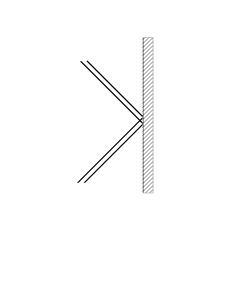
Figure 1: Scattering of a 2-breather from the boundary.

3.3 Soliton boundary $S$ matrix

Although the main focus of this paper is on breather $S$ matrices, we compute here the soliton boundary $S$ matrix in order to further check the identification (3.26) of the boundary parameters.

3.3.1 Attractive case ($\epsilon=-1$)

We consider first the attractive case $\epsilon=-1$, with $\xi_{\pm}$ in the range (3.5), and so the ground state is a sea of negative-parity 1-strings. Following [9],[10], we consider the Bethe Ansatz state consisting of one hole with rapidity $\tilde{\lambda}$ in the sea, which has $S^{z}=+{1\over 2}$. The counting function is

$$h(\lambda) = -{1\over 2\pi}\Bigg{\{}(2N+1)r_{1}(\lambda\,;\mu)+q_{1}(\lambda\,;\mu)+r_{2\xi_{+}-1}(\lambda\,;\mu)+r_{2\xi_{-}-1}(\lambda\,;\mu)$$ (3.27)

$$- \sum_{\beta=1}^{M^{-}_{1}}\left[q_{2}(\lambda-\lambda_{\beta}\,;\mu)+q_{2}(\lambda+\lambda_{\beta}\,;\mu)\right]\Bigg{\}}\,,$$

which leads to the density $\sigma_{s}(\lambda)$ whose Fourier transform is given by

$$\hat{\sigma}_{s}(\omega) = 2\hat{s}(\omega)-{1\over N}\hat{J}(\omega)\left(e^{i\omega\tilde{\lambda}}+e^{-i\omega\tilde{\lambda}}\right)+{1\over N\left(-1+\hat{a}_{2}(\omega\,;\mu)\right)}\bigg{[}\hat{a}_{1}(\omega\,;\mu)$$ (3.28)

$$+ \hat{a}_{2}(\omega\,;\mu)+\hat{b}_{1}(\omega\,;\mu)+\hat{b}_{2\xi_{+}-1}(\omega\,;\mu)+\hat{b}_{2\xi_{-}-1}(\omega\,;\mu)\bigg{]}\,,$$

where $\hat{J}(\omega)$ is defined by

$$\hat{J}(\omega)={\hat{a}_{2}(\omega\,;\mu)\over 1-\hat{a}_{2}(\omega\,;\mu)}={\sinh\left((\nu-2){\omega\over 2}\right)\over 2\sinh\left({\omega\over 2}\right)\cosh\left((\nu-1){\omega\over 2}\right)}\,.$$ (3.29)

We define the boundary $S$ matrix $S(\tilde{\lambda}\,,\xi_{\pm})$ for the soliton by the quantization condition

$$\left(e^{i2p(\tilde{\lambda})N}\ S(\tilde{\lambda}\,,\xi_{-})\ S(\tilde{\lambda}\,,\xi_{+})-1\right)|\tilde{\lambda}\rangle=0\,,$$ (3.30)

where $p(\lambda)$ is given by

$$p(\lambda)=-\left(J*r_{1}\right)(\lambda)-r_{1}(\lambda\,;\mu)\,.$$ (3.31)

The boundary $S$ matrix has the diagonal form

$$S(\tilde{\lambda}\,,\xi_{\pm})=\left(\begin{array}[]{ll}\alpha(\tilde{\lambda}\,,\xi_{\pm})&0\\ 0&\beta(\tilde{\lambda}\,,\xi_{\pm})\end{array}\right)\,.$$ (3.34)

The matrix elements $\alpha(\tilde{\lambda}\,,\xi)$ and $\beta(\tilde{\lambda}\,,\xi)$ are the boundary scattering amplitudes for one-hole states with $S^{z}=+{1\over 2}$ and $S^{z}=-{1\over 2}$, respectively. We compute these matrix elements with the help of the identity

$${1\over\pi}{d\over d\lambda}p(\lambda)+\sigma_{s}(\lambda)-2s(\lambda)-{1\over N}{d\over d\lambda}h(\lambda)=0\,.$$ (3.35)

We first compute $\alpha(\tilde{\lambda}\,,\xi)$. We have (up to a rapidity-independent phase factor)

$$\alpha(\tilde{\lambda}\,,\xi_{+})\ \alpha(\tilde{\lambda}\,,\xi_{-})\sim\exp\left\{i2\pi N\int_{0}^{\tilde{\lambda}}\left(\sigma_{s}(\lambda)-2s(\lambda)\right)d\lambda\right\}\,.$$ (3.36)

Substituting the result (3.28) for the root density and performing some algebra, we obtain

$$\alpha(\tilde{\lambda}\,,\xi) \sim \exp\Bigg{\{}-2\int_{0}^{\infty}{d\omega\over\omega}\sinh\left(2i\omega\tilde{\lambda}\right)\bigg{[}{\sinh\left(3(\nu-1){\omega\over 2}\right)\sinh\left((\nu-2){\omega\over 2}\right)\over\sinh\left({\omega\over 2}\right)\sinh\left(2(\nu-1)\omega\right)}$$ (3.37)

$$- {\sinh\left((2\xi-1)\omega\right)\over 2\sinh\omega\cosh\left((\nu-1)\omega\right)}\bigg{]}\Bigg{\}}$$

$$= {1\over\pi}\cosh[\pi(\tilde{\lambda}+{i\over 2}(2\xi-\nu))]\ S_{0}(\tilde{\lambda})\ S_{1}(\tilde{\lambda}\,,\xi)\,,$$

where

$$S_{0}(\tilde{\lambda}) = \prod_{n=0}^{\infty}\Bigg{\{}{\Gamma\left(-2i\tilde{\lambda}+(\nu-1)(4n+3)+1\right)\Gamma\left(-2i\tilde{\lambda}+(\nu-1)(4n+1)\right)\over\Gamma\left(2i\tilde{\lambda}+(\nu-1)(4n+3)+1\right)\Gamma\left(2i\tilde{\lambda}+(\nu-1)(4n+1)\right)}$$ (3.38)

$$\times {\Gamma\left(2i\tilde{\lambda}+4(\nu-1)n+1\right)\Gamma\left(2i\tilde{\lambda}+4(\nu-1)(n+1)\right)\over\Gamma\left(-2i\tilde{\lambda}+4(\nu-1)n+1\right)\Gamma\left(-2i\tilde{\lambda}+4(\nu-1)(n+1)\right)}\,,$$

and

$$S_{1}(\tilde{\lambda}\,,\xi) = \prod_{n=0}^{\infty}\Bigg{\{}{\Gamma\left(-i\tilde{\lambda}+2(\nu-1)n-{1\over 2}(2\xi-\nu-1)\right)\Gamma\left(-i\tilde{\lambda}+2(\nu-1)n+{1\over 2}(2\xi-\nu+1)\right)\over\Gamma\left(i\tilde{\lambda}+(\nu-1)(2n+2)-{1\over 2}(2\xi-\nu-1)\right)\Gamma\left(i\tilde{\lambda}+(\nu-1)(2n+2)+{1\over 2}(2\xi-\nu+1)\right)}$$

$$\times {\Gamma\left(i\tilde{\lambda}+(\nu-1)(2n+1)-{1\over 2}(2\xi-\nu-1)\right)\Gamma\left(i\tilde{\lambda}+(\nu-1)(2n+1)+{1\over 2}(2\xi-\nu+1)\right)\over\Gamma\left(-i\tilde{\lambda}+(\nu-1)(2n+1)-{1\over 2}(2\xi-\nu-1)\right)\Gamma\left(-i\tilde{\lambda}+(\nu-1)(2n+1)+{1\over 2}(2\xi-\nu+1)\right)}\Bigg{\}}\,.$$

In order to compute $\beta(\tilde{\lambda}\,,\xi)$, we must consider a one-hole state with $S^{z}=-{1\over 2}$. As explained in [9],[10], this can be achieved by working instead with the the pseudovacuum with all spins down, in which case the Bethe Ansatz Eqs. are given by (3.3) with the replacement $\xi_{\pm}\rightarrow-\xi_{\pm}$. The corresponding density $\hat{\sigma}^{\prime}_{s}(\omega)$ is given by Eq. (3.28) with the replacement $\hat{b}_{2\xi_{\pm}-1}(\omega\,;\mu)\rightarrow-\hat{b}_{2\xi_{\pm}+1}(\omega\,;\mu)$. We find

$$\sigma^{\prime}_{s}(\lambda)-\sigma_{s}(\lambda)={1\over N}\left(b_{2\xi_{-}-\nu}(\lambda\,;\pi)+b_{2\xi_{+}-\nu}(\lambda\,;\pi)\right)\,.$$ (3.40)

In obtaining this result, we have noted that for $\xi_{\pm}$ in the range (3.5), the quantities $\hat{b}_{2\xi_{\pm}-1}(\omega\,;\mu)$ and $\hat{b}_{2\xi_{\pm}+1}(\omega\,;\mu)$ are given by Eqs. (2.14) and (2.15), respectively. Since

$${\beta(\tilde{\lambda}\,,\xi_{+})\ \beta(\tilde{\lambda}\,,\xi_{-})\over\alpha(\tilde{\lambda}\,,\xi_{+})\ \alpha(\tilde{\lambda}\,,\xi_{-})}=\exp\left\{i2\pi N\int_{0}^{\tilde{\lambda}}\left(\sigma^{\prime}_{s}(\lambda)-\sigma_{s}(\lambda)\right)d\lambda\right\}\,,$$ (3.41)

we conclude that

$${\beta(\tilde{\lambda}\,,\xi)\over\alpha(\tilde{\lambda}\,,\xi)}={\cosh\left[\pi\left(\tilde{\lambda}-{i\over 2}(2\xi-\nu)\right)\right]\over\cosh\left[\pi\left(\tilde{\lambda}+{i\over 2}(2\xi-\nu)\right)\right]}\,.$$ (3.42)

The soliton boundary $S$ matrix (3.34), (3.37)-(LABEL:s1a),(3.42) agrees with the bootstrap result of Ghoshal-Zamolodchikov [6] for the boundary sine-Gordon model with “fixed” boundary conditions, provided the identification of boundary parameters (3.26) is again made. Fendley-Saleur [8] find a similar identification.

3.3.2 Repulsive case ($\epsilon=+1$)

We consider finally the repulsive case $\epsilon=+1$, where there are no breathers. Here the ground state corresponds to a sea of positive parity 1-strings, i.e., real solutions of the Bethe Ansatz equations. For the Bethe Ansatz state with one hole of rapidity $\tilde{\lambda}$ in the sea, the counting function is

$$h(\lambda) = {1\over 2\pi}\Bigg{\{}(2N+1)q_{1}(\lambda\,;\mu)+r_{1}(\lambda\,;\mu)+q_{2\xi_{+}-1}(\lambda\,;\mu)+q_{2\xi_{-}-1}(\lambda\,;\mu)$$ (3.43)

$$- \sum_{\beta=1}^{M^{-}_{1}}\left[q_{2}(\lambda-\lambda_{\beta}\,;\mu)+q_{2}(\lambda+\lambda_{\beta}\,;\mu)\right]\Bigg{\}}\,,$$

and the density $\sigma_{s}(\lambda)$ is given by

$$\hat{\sigma}_{s}(\omega) = 2\hat{s}(\omega)+{1\over N}\hat{J}(\omega)\left(e^{i\omega\tilde{\lambda}}+e^{-i\omega\tilde{\lambda}}\right)+{1\over N\left(1+\hat{a}_{2}(\omega\,;\mu)\right)}\bigg{[}\hat{a}_{1}(\omega\,;\mu)$$ (3.44)

$$+ \hat{a}_{2}(\omega\,;\mu)+\hat{b}_{1}(\omega\,;\mu)+\hat{a}_{2\xi_{+}-1}(\omega\,;\mu)+\hat{a}_{2\xi_{-}-1}(\omega\,;\mu)\bigg{]}\,,$$

where now

$$\hat{s}(\omega) = {\hat{a}_{1}(\omega\,;\mu)\over 1+\hat{a}_{2}(\omega\,;\mu)}={1\over 2\cosh\left({\omega\over 2}\right)}\,,$$

$$\hat{J}(\omega) = {\hat{a}_{2}(\omega\,;\mu)\over 1+\hat{a}_{2}(\omega\,;\mu)}={\sinh\left((\nu-2){\omega\over 2})\right)\over 2\sinh\left((\nu-1){\omega\over 2}\right)\cosh\left({\omega\over 2}\right)}\,.$$ (3.45)

Moreover, in the repulsive case,

$$p(\lambda)=-\left(J*q_{1}\right)(\lambda)+q_{1}(\lambda\,;\mu)\,.$$ (3.46)

Proceeding as in the attractive case, we find that the soliton boundary $S$ matrix has the form (3.34) with matrix elements

$$\alpha(\tilde{\lambda}\,,\xi) \sim \exp\Bigg{\{}2\int_{0}^{\infty}{d\omega\over\omega}\sinh\left(2i\omega\tilde{\lambda}\right)\bigg{[}{\sinh\left({3\omega\over 2}\right)\sinh\left((\nu-2){\omega\over 2}\right)\over\sinh\left(2\omega\right)\sinh\left((\nu-1){\omega\over 2}\right)}$$ (3.47)

$$+ {\sinh\left((\nu-2\xi+1)\omega\right)\over 2\sinh\left((\nu-1)\omega\right)\cosh\omega}\bigg{]}\Bigg{\}}$$

$$= {1\over\pi}\cosh[{\pi\over\nu-1}(\tilde{\lambda}+{i\over 2}(\nu-2\xi))]\ S_{0}(\tilde{\lambda})\ S_{1}(\tilde{\lambda}\,,\xi)\,,$$

where

$$S_{0}(\tilde{\lambda}) = \prod_{n=0}^{\infty}\Bigg{\{}{\Gamma\left({1\over\nu-1}(-2i\tilde{\lambda}+4n+3)+1\right)\Gamma\left({1\over\nu-1}(-2i\tilde{\lambda}+4n+1)\right)\over\Gamma\left({1\over\nu-1}(2i\tilde{\lambda}+4n+3)+1\right)\Gamma\left({1\over\nu-1}(2i\tilde{\lambda}+4n+1)\right)}$$ (3.48)

$$\times {\Gamma\left({1\over\nu-1}(2i\tilde{\lambda}+4n)+1\right)\Gamma\left({1\over\nu-1}(2i\tilde{\lambda}+4n+4)\right)\over\Gamma\left({1\over\nu-1}(-2i\tilde{\lambda}+4n)+1\right)\Gamma\left({1\over\nu-1}(-2i\tilde{\lambda}+4n+4)\right)}\,,$$

$$S_{1}(\tilde{\lambda}\,,\xi) = \prod_{n=0}^{\infty}\Bigg{\{}{\Gamma\left({1\over\nu-1}(-i\tilde{\lambda}+2n-{1\over 2}(\nu-2\xi))+{1\over 2}\right)\Gamma\left({1\over\nu-1}(-i\tilde{\lambda}+2n+{1\over 2}(\nu-2\xi))+{1\over 2}\right)\over\Gamma\left({1\over\nu-1}(i\tilde{\lambda}+2n+2-{1\over 2}(\nu-2\xi))+{1\over 2}\right)\Gamma\left({1\over\nu-1}(i\tilde{\lambda}+2n+2+{1\over 2}(\nu-2\xi))+{1\over 2}\right)}$$

$$\times {\Gamma\left({1\over\nu-1}(i\tilde{\lambda}+2n+1-{1\over 2}(\nu-2\xi))+{1\over 2}\right)\Gamma\left({1\over\nu-1}(i\tilde{\lambda}+2n+1+{1\over 2}(\nu-2\xi))+{1\over 2}\right)\over\Gamma\left({1\over\nu-1}(-i\tilde{\lambda}+2n+1-{1\over 2}(\nu-2\xi))+{1\over 2}\right)\Gamma\left({1\over\nu-1}(-i\tilde{\lambda}+2n+1+{1\over 2}(\nu-2\xi))+{1\over 2}\right)}\Bigg{\}}\,,$$

and

$${\beta(\tilde{\lambda}\,,\xi)\over\alpha(\tilde{\lambda}\,,\xi)}={\cosh\left[{\pi\over\nu-1}\left(\tilde{\lambda}-{i\over 2}(\nu-2\xi)\right)\right]\over\cosh\left[{\pi\over\nu-1}\left(\tilde{\lambda}+{i\over 2}(\nu-2\xi)\right)\right]}\,.$$ (3.50)

Comparing with Ghoshal-Zamolodchikov [6], we obtain the following identification of boundary parameters

$$x={\pi\left(\nu-2\xi^{(+1)}\right)\over 2(\nu-1)}\,.$$ (3.51)

The same identification was found in [8]. We remark that, by setting

$$\mu^{\prime}=\pi-\mu\,,\qquad\xi^{\prime}=-{\xi^{(-1)}\over\nu-1}\,,$$ (3.52)

as in Appendix A, the formula (3.26) for $x$ in the attractive case can be recast in the similar form

$$x={\pi\left(-\nu^{\prime}-2\xi^{\prime}\right)\over 2(\nu^{\prime}-1)}\,,$$ (3.53)

where $\nu^{\prime}={\pi\over\mu^{\prime}}$.

4 Discussion

We have formulated a systematic Bethe-Ansatz approach for computing breather $S$ matrices for integrable quantum spin chains. We have used this approach to calculate the breather boundary $S$ matrix for the open XXZ spin chain with diagonal boundary fields. We have also directly computed the soliton boundary $S$ matrix in the critical regime.

Let us briefly compare our approach with that of other authors. Our approach is essentially a systematization of Korepin’s [2] analysis of the massive Thirring model. Key elements of our approach are the exploitation of the “second” set of Bethe Ansatz Eqs. (LABEL:bulk/string) which describes the centers of the breather strings; and the use of the identity (2.43). An analogous identity for holes was used by Andrei and Destri [3] to compute soliton $S$ matrices. Fendley and Saleur [8] study boundary $S$ matrices of the XXZ chain using an alternative approach based on the model’s physical Bethe Ansatz equations [11]. The identification of boundary $S$ matrices from the physical Bethe Ansatz Eqs. is not straightforward, especially in the repulsive case. Finally, we remark that the vertex-operator approach [18] has so far been restricted in applicability to the noncritical regime.

While we have focused on the XXZ chain for simplicity, we expect that the same methods should be applicable to other models. Indeed, boundary $S$ matrices for the critical $A_{\mathcal{N}-1}^{(1)}$ open spin chain with diagonal boundary fields can be computed in this way [19].

Appendix A Dependence on $\epsilon$

Following many authors (see, e.g., [8],[11],[13], ), we treat the full critical regime of the XXZ chain by restricting the anisotropy parameter $\mu$ to the range $(0\,,{\pi\over 2})$, and introducing a new parameter $\epsilon=\pm 1$. We describe here this approach in detail, since there are some subtleties associated with it, such as the dependence on $\epsilon$ in the expression (2.6) for the momentum and in the boundary parameters.

A.1 Closed chain

We take as our starting point the following definition of the critical XXZ closed chain Hamiltonian

$${\cal H}={1\over 4}\sum_{n=1}^{N}\left\{\sigma^{x}_{n}\sigma^{x}_{n+1}+\sigma^{y}_{n}\sigma^{y}_{n+1}+\cos\mu^{\prime}\left(\sigma^{z}_{n}\sigma^{z}_{n+1}-1\right)\right\}\,,$$ (A.1)

with $0<\mu^{\prime}<\pi$. The repulsive regime corresponds to $0<\mu^{\prime}<{\pi\over 2}$, while the attractive regime corresponds to ${\pi\over 2}<\mu^{\prime}<\pi$. The standard algebraic Bethe Ansatz procedure gives

$$E = -\sin^{2}\mu^{\prime}\sum_{\alpha=1}^{M}{1\over\cosh(2\mu^{\prime}\lambda^{\prime}_{\alpha})-\cos\mu^{\prime}}\,,$$ (A.2)

$$P = +{1\over i}\sum_{\alpha=1}^{M}\log{\sinh\mu^{\prime}\left(\lambda^{\prime}_{\alpha}+{i\over 2}\right)\over\sinh\mu^{\prime}\left(\lambda^{\prime}_{\alpha}-{i\over 2}\right)}\quad(\mbox{mod }2\pi)\,,$$ (A.3)

with

$$\left({\sinh\mu^{\prime}\left(\lambda^{\prime}_{\alpha}+{i\over 2}\right)\over\sinh\mu^{\prime}\left(\lambda^{\prime}_{\alpha}-{i\over 2}\right)}\right)^{N}=\prod_{\scriptstyle{\beta=1}\atop\scriptstyle{\beta\neq\alpha}}^{M}{\sinh\mu^{\prime}\left(\lambda^{\prime}_{\alpha}-\lambda^{\prime}_{\beta}+i\right)\over\sinh\mu^{\prime}\left(\lambda^{\prime}_{\alpha}-\lambda^{\prime}_{\beta}-i\right)}\,,\quad\alpha=1\,,\cdots\,,M\,.$$ (A.4)

These are simply the formulas of Section 2 for $\epsilon=+1$ with primes appended to $\mu$ and $\lambda_{\alpha}$.

The principal observation is that the “duality” transformation

$$\mu = \pi-\mu^{\prime}$$

$$\lambda_{\alpha} = {\mu^{\prime}\over\mu}\lambda^{\prime}_{\alpha}+{i\pi\over 2\mu}$$ (A.5)

implies

$${\cal H}={1\over 4}\sum_{n=1}^{N}\left\{\sigma^{x}_{n}\sigma^{x}_{n+1}+\sigma^{y}_{n}\sigma^{y}_{n+1}-\cos\mu\left(\sigma^{z}_{n}\sigma^{z}_{n+1}-1\right)\right\}\,,$$ (A.6)

$$E = +\sin^{2}\mu\sum_{\alpha=1}^{M}{1\over\cosh(2\mu\lambda_{\alpha})-\cos\mu}\,,$$ (A.7)

$$P = \pi M-{1\over i}\sum_{\alpha=1}^{M}\log{\sinh\mu\left(\lambda_{\alpha}+{i\over 2}\right)\over\sinh\mu\left(\lambda_{\alpha}-{i\over 2}\right)}\quad(\mbox{mod }2\pi)\,,$$ (A.8)

with

$$\left(-{\sinh\mu\left(\lambda_{\alpha}+{i\over 2}\right)\over\sinh\mu\left(\lambda_{\alpha}-{i\over 2}\right)}\right)^{N}=\prod_{\scriptstyle{\beta=1}\atop\scriptstyle{\beta\neq\alpha}}^{M}{\sinh\mu\left(\lambda_{\alpha}-\lambda_{\beta}+i\right)\over\sinh\mu\left(\lambda_{\alpha}-\lambda_{\beta}-i\right)}\,,\quad\alpha=1\,,\cdots\,,M\,.$$ (A.9)

The proof relies on elementary identities $\sinh\mu(\lambda_{\alpha}+{i\over 2})=-\sinh\mu^{\prime}(\lambda^{\prime}_{\alpha}-{i\over 2})$, $\sinh\mu(\lambda_{\alpha}-{i\over 2})=\sinh\mu^{\prime}(\lambda^{\prime}_{\alpha}+{i\over 2})$, etc.

The Bethe Ansatz Eqs. remain invariant under the transformation (A.5) for $N$ even. Evidently, the attractive regime (${\pi\over 2}<\mu^{\prime}<\pi$) corresponds to $0<\mu<{\pi\over 2}$. The expressions (A.7),(A.8) coincide with the corresponding formulas of Section 2 with $\epsilon=-1$. Moreover, as is well-known [12], the Hamiltonian (A.6) with $N$ even can be mapped by a unitary transformation to the Hamiltonian (2.1) with $\epsilon=-1$.

A.2 Open chain

We define the critical XXZ open chain Hamiltonian by

$${\cal H}={1\over 4}\left\{\sum_{n=1}^{N-1}\left(\sigma^{x}_{n}\sigma^{x}_{n+1}+\sigma^{y}_{n}\sigma^{y}_{n+1}+\cos\mu^{\prime}\ \sigma^{z}_{n}\sigma^{z}_{n+1}\right)+\sin\mu^{\prime}\cot(\mu^{\prime}\xi^{\prime}_{-})\sigma^{z}_{1}+\sin\mu^{\prime}\cot(\mu^{\prime}\xi^{\prime}_{+})\sigma^{z}_{N}\right\}\,,$$

with $0<\mu^{\prime}<\pi$. The corresponding Bethe Ansatz Eqs. remain invariant under the transformation (A.5) for any $N$ provided there is an accompanying transformation of the boundary parameters,

$$\xi_{\pm}=-{\mu^{\prime}\over\mu}\xi^{\prime}_{\pm}=-(\nu-1)\xi^{\prime}_{\pm}\,.$$ (A.11)

It follows that the Hamiltonian is equal to

$${\cal H}={1\over 4}\left\{\sum_{n=1}^{N-1}\left(\sigma^{x}_{n}\sigma^{x}_{n+1}+\sigma^{y}_{n}\sigma^{y}_{n+1}-\cos\mu\ \sigma^{z}_{n}\sigma^{z}_{n+1}\right)-\sin\mu\cot(\mu\xi_{-})\sigma^{z}_{1}-\sin\mu\cot(\mu\xi_{+})\sigma^{z}_{N}\right\}\,,$$

which for any $N$ can be mapped by a unitary transformation to

$${\cal H}=-{1\over 4}\left\{\sum_{n=1}^{N-1}\left(\sigma^{x}_{n}\sigma^{x}_{n+1}+\sigma^{y}_{n}\sigma^{y}_{n+1}+\cos\mu\ \sigma^{z}_{n}\sigma^{z}_{n+1}\right)+\sin\mu\cot(\mu\xi_{-})\sigma^{z}_{1}+\sin\mu\cot(\mu\xi_{+})\sigma^{z}_{N}\right\}\,.$$

We conclude that the critical open chain can also be described by the Hamiltonian (3.1) with $0<\mu<{\pi\over 2}$ and $\epsilon=\pm 1$, where

$$\xi_{\pm}^{(+1)} = \xi^{\prime}_{\pm}$$

$$\xi_{\pm}^{(-1)} = -(\nu-1)\xi^{\prime}_{\pm}\,.$$ (A.14)

Appendix B Boundary 1-strings

The existence of boundary string solutions of the open-chain Bethe Ansatz equations was discussed in Ref. [16]. For completeness, we demonstrate here the existence of boundary 1-strings following the approach used by Faddeev and Takhtajan [17] to study bulk 2-strings. We therefore consider Eq. (3.3) for the case $M=1$ with $N\rightarrow\infty$,

$$\left({\sinh\mu\left(\lambda+{i\over 2}\right)\over\sinh\mu\left(\lambda-{i\over 2}\right)}\right)^{2N}{\sinh\mu\left(\lambda+i(\xi-{1\over 2})\right)\over\sinh\mu\left(\lambda-i(\xi-{1\over 2})\right)}=1\,.$$ (B.1)

For simplicity, we have written boundary terms from just one boundary. Setting $\lambda=x+iy$ with $x$, $y$ real,

$$\left({\sinh\mu\left(x+i(y+{1\over 2})\right)\over\sinh\mu\left(x+i(y-{1\over 2})\right)}\right)^{2N}{\sinh\mu\left(x+i(y+\xi-{1\over 2})\right)\over\sinh\mu\left(x+i(y-\xi+{1\over 2})\right)}=1\,.$$ (B.2)

Multiplying by the complex conjugate and using the identity $\sinh(a+ib)\ \sinh(a-ib)=\sinh^{2}a+\sin^{2}b$, we obtain

$$A^{2N}\ B=1\,,$$ (B.3)

where

$$A={\sinh^{2}\mu x+\sin^{2}\mu(y+{1\over 2})\over\sinh^{2}\mu x+\sin^{2}\mu(y-{1\over 2})}\,,\qquad B={\sinh^{2}\mu x+\sin^{2}\mu(y+\xi-{1\over 2})\over\sinh^{2}\mu x+\sin^{2}\mu(y-\xi+{1\over 2})}\,.$$ (B.4)

Evidently, there is a periodicity $y\rightarrow y+{\pi\over\mu}$. We therefore consider two cases:

• Case I:

  $$0<y<{\pi\over 2\mu}\quad(\mbox{mod }{\pi\over\mu})$$ (B.5)

  It follows that $\sin^{2}\mu(y+{1\over 2})>\sin^{2}\mu(y-{1\over 2})$; therefore $A>1$, and hence $A^{2N}\rightarrow\infty$ for $N\rightarrow\infty$. Eq. (B.3) then implies $B\rightarrow 0$. That is, for $N\rightarrow\infty$,

  $$x=0\,,\qquad y=-(\xi-{1\over 2})\quad(\mbox{mod }{\pi\over\mu})\,.$$ (B.6)

  The restriction (B.5) then implies

  $${1\over 2}-{\pi\over 2\mu}<\xi<{1\over 2}\quad(\mbox{mod }{\pi\over\mu})\,.$$ (B.7)

• Case II:

  $$-{\pi\over 2\mu}<y<0\quad(\mbox{mod }{\pi\over\mu})$$ (B.8)

  Then $\sin^{2}\mu(y+{1\over 2})<\sin^{2}\mu(y-{1\over 2})$; therefore $A<1$, and hence $A^{2N}\rightarrow 0$ for $N\rightarrow\infty$. Eq. (B.3) then implies $B\rightarrow\infty$. That is, for $N\rightarrow\infty$,

  $$x=0\,,\qquad y=\xi-{1\over 2}\quad(\mbox{mod }{\pi\over\mu})\,.$$ (B.9)

  The restriction (B.8) leads again to the condition (B.7).

In conclusion, the Bethe Ansatz Eqs. have the boundary 1-string solutions $\lambda=\pm i\left(\xi-{1\over 2}\right)$ when $\xi$ satisfies the condition (B.7). Boundary strings of longer length are also studied in [16].

References

- [1] A.B. Zamolodchikov and Al.B. Zamolodchikov, Ann. Phys. 120 (1979) 253.
- [2] V.E. Korepin, Theor. Math. Phys. 41 (1979) 953.
- [3] N. Andrei and C. Destri, Nucl. Phys. B231 (1984) 445.
- [4] F.C. Alcaraz, M.N. Barber, M.T. Batchelor, R.J. Baxter and G.R.W. Quispel, J. Phys. A20 (1987) 6397.
- [5] E.K. Sklyanin, J. Phys. A21 (1988) 2375.
- [6] S. Ghoshal and A. B. Zamolodchikov, Int. J. Mod. Phys. A9 (1994) 3841; A9 (1994) 4353.
- [7] S. Ghoshal, Int. J. Mod. Phys. A9 (1994) 4801.
- [8] P. Fendley and H. Saleur, Nucl. Phys. B428 (1994) 681.
- [9] M. Grisaru, L. Mezincescu and R.I. Nepomechie, J. Phys. A28 (1995) 1027.
- [10] A. Doikou, L. Mezincescu and R.I. Nepomechie, J. Phys. A30 (1997) L507; A31 (1998) 53.
- [11] A.N. Kirillov and N.Yu. Reshetikhin, J. Phys. A20 (1987) 1565.
- [12] J. des Cloizeaux and M. Gaudin, J. Math. Phys. 7 (1966) 1384.
- [13] M. Takahashi and M. Suzuki, Prog. Theor. Phys. 48 (1972) 2187.
- [14] A. Doikou and R.I. Nepomechie, J. Phys. A31 (1998) L621; in Statistical Physics on the Eve of the Twenty-First Century, in press, hep-th/9810034
- [15] L.D. Faddeev and L.A. Takhtajan, Russ. Math. Surv. 34 (1979) 11; P.P. Kulish and E.K. Sklyanin, in Lecture Notes in Physics, v. 151, (Springer, 1982) 61; V.E. Korepin, N.M. Bogoliubov, and A.G. Izergin, Quantum Inverse Scattering Method, Correlation Functions and Algebraic Bethe Ansatz (Cambridge University Press, 1993)
- [16] S. Skorik and H. Saleur, J. Phys. A28 (1995) 6605.
- [17] L.D. Faddeev and L.A. Takhtajan, J. Sov. Math. 24 (1984) 241.
- [18] M. Jimbo and T. Miwa, Algebraic Analysis of Solvable Lattice Models, CBMS Regional Conference Series in Mathematics vol. 85, (AMS, 1994); M. Jimbo, R. Kedem, T. Kojima, H. Konno and T. Miwa, Nucl. Phys. B441 (1995) 437.
- [19] A. Doikou and R.I. Nepomechie, in preparation.